Article

Denitrification Control in a Recirculating Aquaculture System—A Simulation Study

Systems, Estimation, Control and Optimization (SECO), University of Mons, 31, Boulevard Dolez, 7000 Mons, Belgium
*
Author to whom correspondence should be addressed.
Processes 2020, 8(10), 1306; https://doi.org/10.3390/pr8101306
Submission received: 4 September 2020 / Revised: 8 October 2020 / Accepted: 9 October 2020 / Published: 17 October 2020
(This article belongs to the Special Issue Wastewater Treatment Processes)

Abstract

:
The recirculating aquaculture system (RAS) is a land-based water treatment technology, which allows for farming aquatic organisms, such as fish, by reusing the water in the production (often less than 5%). This technology is based on the use of filters, either mechanical or biological, and can, in principle, be used for any species grown in aquaculture. Due to the low recirculation rate, ammonia accumulates in the system and must be converted into nitrate using nitrification reactors. Although less toxic for fish, nitrate can also be further reduced into nitrogen gas by the use of denitrification biofilters which may create several issues, such as incomplete denitrification, resulting in toxic substances, such as nitrite and nitric oxide, or a waste of carbon source in excess. Control of the added quantity of carbon source in the denitrification biofilter is then mandatory to keep nitrate/nitrite concentrations under toxic levels for fish and in accordance with local effluent regulations, and to reduce costs related to wasted organic carbon sources. This study therefore investigates the application of different control methodologies to a denitrification reactor in a RAS. To this end, a numerical simulator is built to predict the RAS behavior and to allow for the comparison of different control approaches, in the presence of changes in the operating conditions, such as fish density and biofilter removal efficiency. First, a classical proportional-integral-derivative (PID) controller was designed, based on an SIMC tuning method depending on the amount of ammonia excreted by fish. Then, linearizing and cascade controllers were considered as possible alternatives.

1. Introduction

Recirculating Aquaculture Systems (RAS) have been increasingly used due to the growth of the aquaculture industry [1]. They can be defined as systems where less than 10% of the total water volume is replaced per day and respond to the need of more intensive practices, growing environmental constraints on water consumption and effluent quality, as well as the possibility to supply fish in places where it would be otherwise difficult [2,3]. The main drawback of these systems is the accumulation of some toxic compounds, such as ammonia, when there is no proper treatment. Ammonia can be introduced into the system by fish excretion, 60–70% of the nitrogen consumption by fish being excreted as ammonia through the gills, or the degradation of uneaten feed [4]. The nitrogen removal process reduces the ammonia level using microorganisms that transform it into nitrate (nitrification). The latter, although much less toxic for fish, also accumulates in the system and needs to be removed to avoid system sustainability and environmental issues. Thus, another unit is often considered in order to convert nitrate into nitrogen gas (denitrification). The use of anaerobic denitrification to remove nitrate is not yet widely applied to commercial RAS due to its level of efficiency, its complexity and cost [5]. The complexity of RAS, created by its intrinsic closed-loop and the interactions between water treatment and fish grow-out, implies to build dynamic models to analyze the process behavior and to optimize it (configuration, size, fish, feed, flows etc) with respect to cost, robustness and water quality [6]. Indeed, manual control of denitrifying biofilters may easily lead to an unstable process performance and high cost [7]. Nitrite, which is toxic for fish, can accumulate in transient phases [8]. It is an intermediate compound in the denitrification process, a set of four reactions converting nitrate N O 3 to nitrogen N 2 . Particularly, the lack of carbon source for complete denitrification could make this problem more severe. The absence of nitrite/nitrate/oxygen, however, if large quantities of organic matter exist, causes the production of sulfides (such as hydrogen sulfide) which are also extremely toxic [9]. Although nitrate control has been addressed many times regarding municipal wastewater treatment, its application in the context of RAS is not widespread [7,10,11,12]. A multivariable PID control, manipulating recirculation flowrates and aeration to control nitrate levels is proposed in [12] while an online control strategy/algorithm optimizing a denitrification biofilter through carbon dosage and backwash is shown in [7]. In [10], a simple feedback control strategy by methanol addition is used to minimize nitrite production and [11] proposes an output-feedback control scheme for a wastewater treatment biofilters in order to regulate nitrate and nitrite concentrations.
In this study, a global assessment of nitrate control using acetic acid (pH is considered regulated and constant) as manipulated variable is first achieved and two different control methodologies are considered: a classical PID control whose parameters are estimated by a SIMC tuning method [13], and a simple model-based linearizing control. PID control is widely used in process industries [14], and have been extensively used to control WWTPs. Unfortunately, PID controllers may present robustness limitations when applied to nonlinear systems with modeling uncertainties as well as measurement noise. They might indeed require tuning each time the operating conditions significantly vary. Linear controllers, on the other hand, take advantage of the availability of accurate nonlinear models often based on reaction networks and mass balances. However, as bioprocess models generally present uncertain kinetic structures, adaptive and/or robust solutions are required [15,16,17,18]. Taking advantage of both controller structures, a cascade of PI and linearizing control (accounting for possible model inaccuracies) is further proposed and compared with an adaptive linearizing strategy. The controller performances are tested with regard to typical industrial plant variations: changes in fish density, biofilter nitrate conversion efficiency, effluent guidelines regarding nitrate and water/acid pump malfunction in the denitrification reactor.

2. Problem Description

2.1. Industrial Plant

The industrial-scale RAS under consideration was composed of fish tanks, a physical filtration system and two biofilters (one for nitrification and another for denitrification). The reactor sizes and flowrates are presented in Figure 1.
The fish were reared in the tanks from where water flowed into a physical filtration system in order to remove particles. This water flow was then bypassed by a denitrification system where a carbon source, acetic acid, was injected. The nitrification filter was composed of 6 compartments, each one filled with fixed plastic support. Oxygen was added to the nitrification filter up to its saturation point and fresh water could also have been introduced in the system at a rate F f r e s h .
In the following analyses, the RAS system is assumed to operate at a specific setpoint and model-based control strategies are designed to allow the user to choose specific operating conditions (i.e., to keep the current setpoint in steady-state or to chose another setpoint) and the closed-loop system to compensate possible disturbances. Regarding the simulated industrial plant, the nominal steady-state corresponds to a 6.4 L/h acetic acid flow rate ( F A c i d ¯ ) added to keep a constant nitrate concentration in the denitrification biofilter of 26.6 gN/m3. Water leaves the fish basins (and enters the denitrification biofilter) with oxygen, ammonium and nitrate concentrations of, respectively, 6.8 gCOD/m3, 0.5 gN/m3 and 98 gN/m3.

2.2. Model Description

Each block of the industrial RAS is described by the following models whose components and nomenclature are related to the Activated Sludge Models (ASM) from [19].
  • Fish Tanks:
    The fish excretion rate is considered with assumed constant fish size and population. It can be translated into ASM variables using the waste matrix reported in [6]. The fish respiration is calculated based on the values reported in [20,21] (see Table 1).
    The Fish basins are modeled as perfectly mixed tank reactors where no biological reaction occurs, applying mass balances as in:
    d ξ d t = D ( ξ i n l e t ξ ) + ϑ w a s t e V
    where variable ξ may be used to represent both soluble (S) and particulate (X) waste compounds and V is the fish tank volume. The corresponding waste production rates ϑ w a s t e , all quantified in Table 1, are estimated for an assumed constant fish density of 12 kg/m3 and body weight of 8.5 kg. These rates can also be translated into ASM variables using the waste matrix reported in [6] while the fish respiration is calculated based on the values reported in [20,21] (see Table 1). The fish basin may therefore be modeled by the replication of the generic Equation (1) for each waste component of Table 1.
  • Physical particle filter:
    90% of the particulate components in the inlet are filtered, leading to:
    X k , o u t l e t = 0.1 X k , i n l e t
    where X k , o u t l e t and X k , i n l e t represent, respectively, the outlet and inlet concentrations of particulate component k.
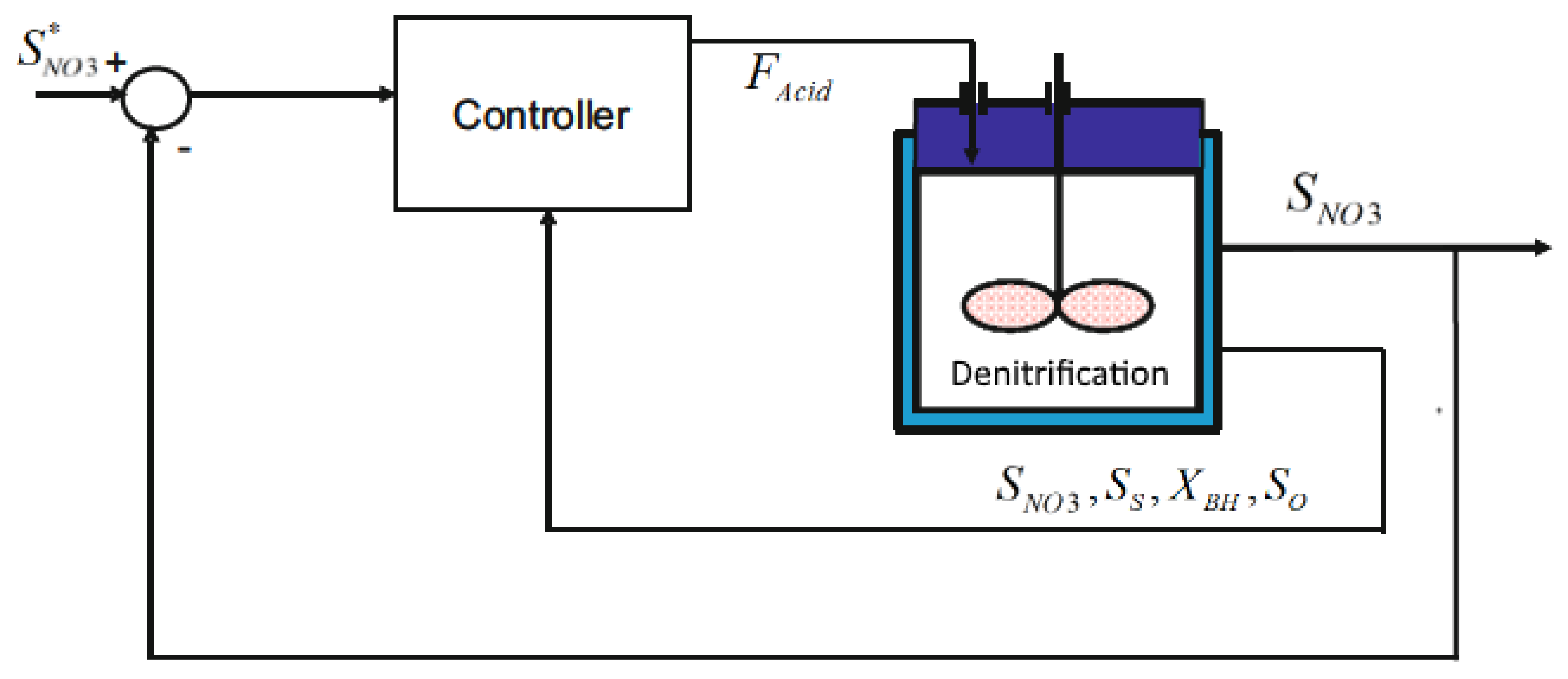
  • Denitrification filter:
    The denitrification filter consists of a moving bed perfectly-mixed tank reactor. Solubles that exist in the reactor bulk (index b) dissolve into the biofilm (index c) where the main part of the biological reactions occurs. The same ASM model, which is applied for nitrification, is used with the exception that ammonia is not considered as substrate for heterotrophic growth ( S N H ( K N H H + S N H ) is not considered in ρ 1 , ρ 2 and ρ 3 ). Acetic acid is added to this bioreactor (4) as a carbon source for denitrification, which can therefore be modeled as:
    d S i , b d t = D ( S i , i n l e t S i , b ) + m ˙ i , A d d e d V b k d i f f ( S i , b S i , c ) V b + ϕ S i , b
    m ˙ S S , A d d e d = F A c i d φ
    d X k , b d t = D ( X k , i n l e t X k , b ) + K d V b X k , c + ϕ X k , b
    d S i , c d t = k d i f f V b f ( S i , b S i , c ) + ϕ S i , c
    d X k , c d t = K d V b f X k , c + ϕ X k , c
    where F A c i d is the acetic acid flow rate in L / h , φ is the coefficient of conversion of acid into easily biodegradable organic matter in g C O D / L and ϕ ξ is the production/consumption rate of component ξ, which can be calculated using stoichiometry—that is, the corresponding coefficient υ ξ , w (provided in Table S1, in Supplementary Materials) and rate ρ w (provided in Table S2, in Supplementary Materials), as in:
    ϕ ξ = w = 1 11 υ ξ , w × ρ w
    where w is an index denoting the process referenced in Tables S1 and S2 in Supplementary Materials.
  • Nitrification filter:
    The nitrification filter is hydraulically modeled assuming six sequential perfectly mixed tank reactors filled with solid media. Biologically, a modified ASM1 model with the inclusion of two-step nitrification/denitrification is used (provided in Tables S1 and S2, in Supplementary Materials). This model has been validated using the data from the COST Simulation Benchmark in [22]. It has to be noticed that oxygen is also added to this bioreactor. Particles present in the inlet remain in the outlet. However, the particles already existing in each compartment ( r s ) do not move to others. The resulting mass balances lead to:
    d S i , r s d t = F V b ( S i , r s 1 S i , r s ) + m ˙ O 2 , A d d e d V b ± ϕ S i , r s V b i o f i l m V b
    d X k , r s d t = ϕ X k , r s
    m ˙ O 2 , A d d e d = k L a ( S O , s a t S O )
    S i , r s 1 = S i , i n l e t , a t r s = 1
    where D represents the dilution rate, k d i f f is the diffusion coefficient in m3/h, V b is the empty volume of the reactor in m3, ϕ S i , r s and ϕ X k , r s are the consumption/production rates of solubles i and particulates k, calculated from (8), F is the volumetric flowrate in m3/h, m ˙ is the mass flowrate in g/h, K d is the detachment coefficient in h−1·m3 and k L a is the oxygen mass transfer coefficient in h−1.

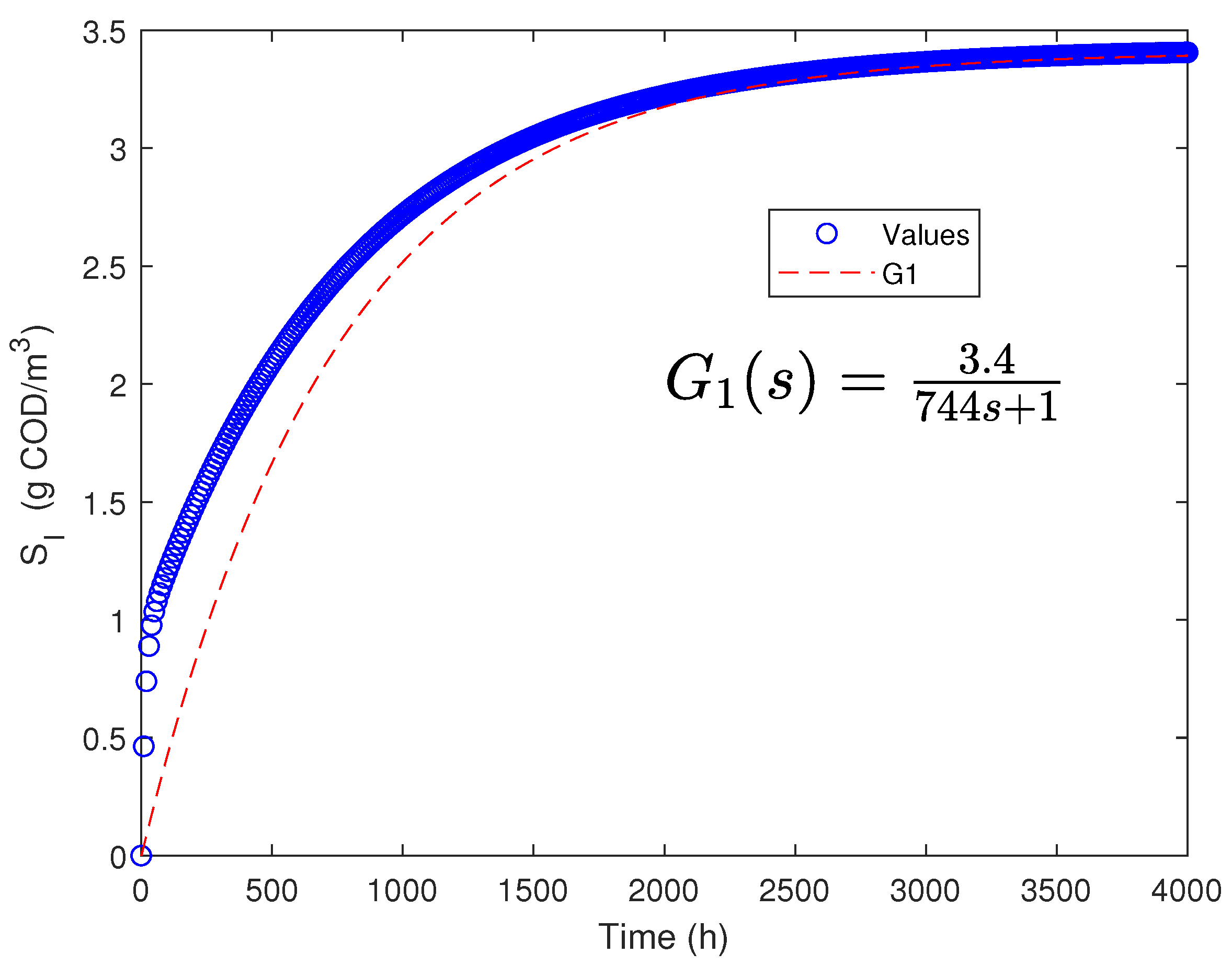
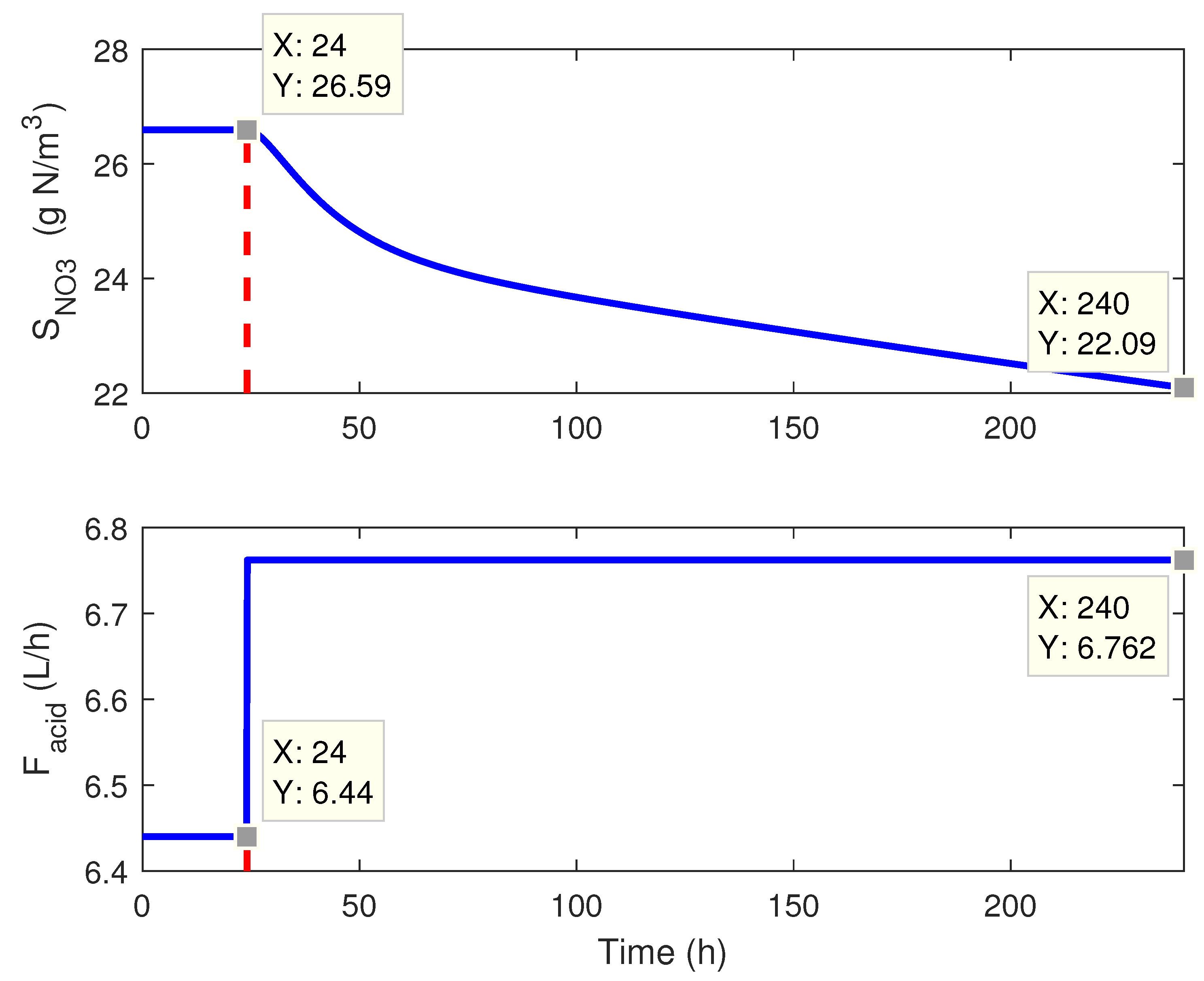
2.3. Plant Dynamics: A Preliminary Study

A first hydraulic study of the plant is achieved in order to assess the RAS inherent dynamics. To this end, a simulation of the concentration variation of an inert soluble component in the denitrification reactor following a production rate unitary step increase (in gCOD/(m3·h)) is shown in Figure 2 where, obviously, the plant takes up to 4000 h to reach the new steady state. Indeed, the step response can be approximated using a first order transfer function G 1 with time constant τ C = 744 h—i.e., 5 τ C 4000 h. As already mentioned, the plant is a semi closed system with 1% of regenerated water flowrate. This small inlet of water, along with the high considered volume, causes the very slow drift towards the new steady-state. This preliminary numerical analysis aims at demonstrating that the current RAS is very delicate to control due to the recirculating loop dynamics. In the upcoming sections, dedicated to control design, these slow dynamics are taken into account using adapted controller settings.

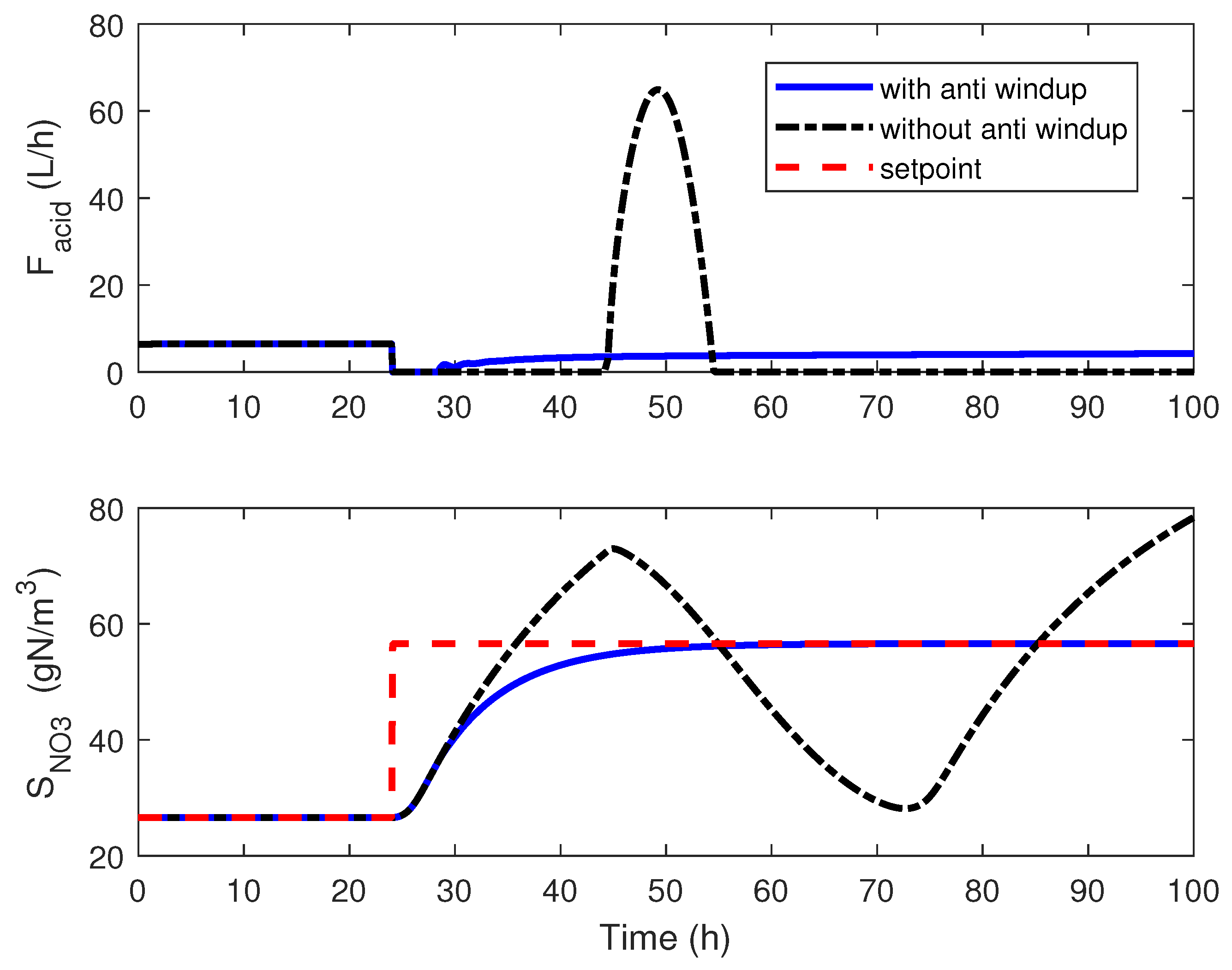
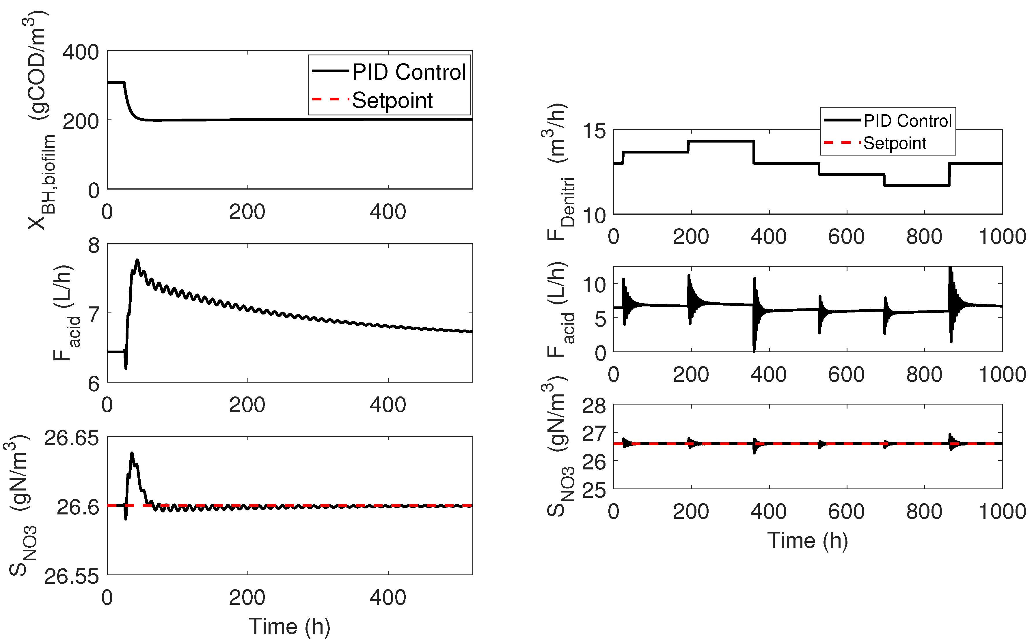
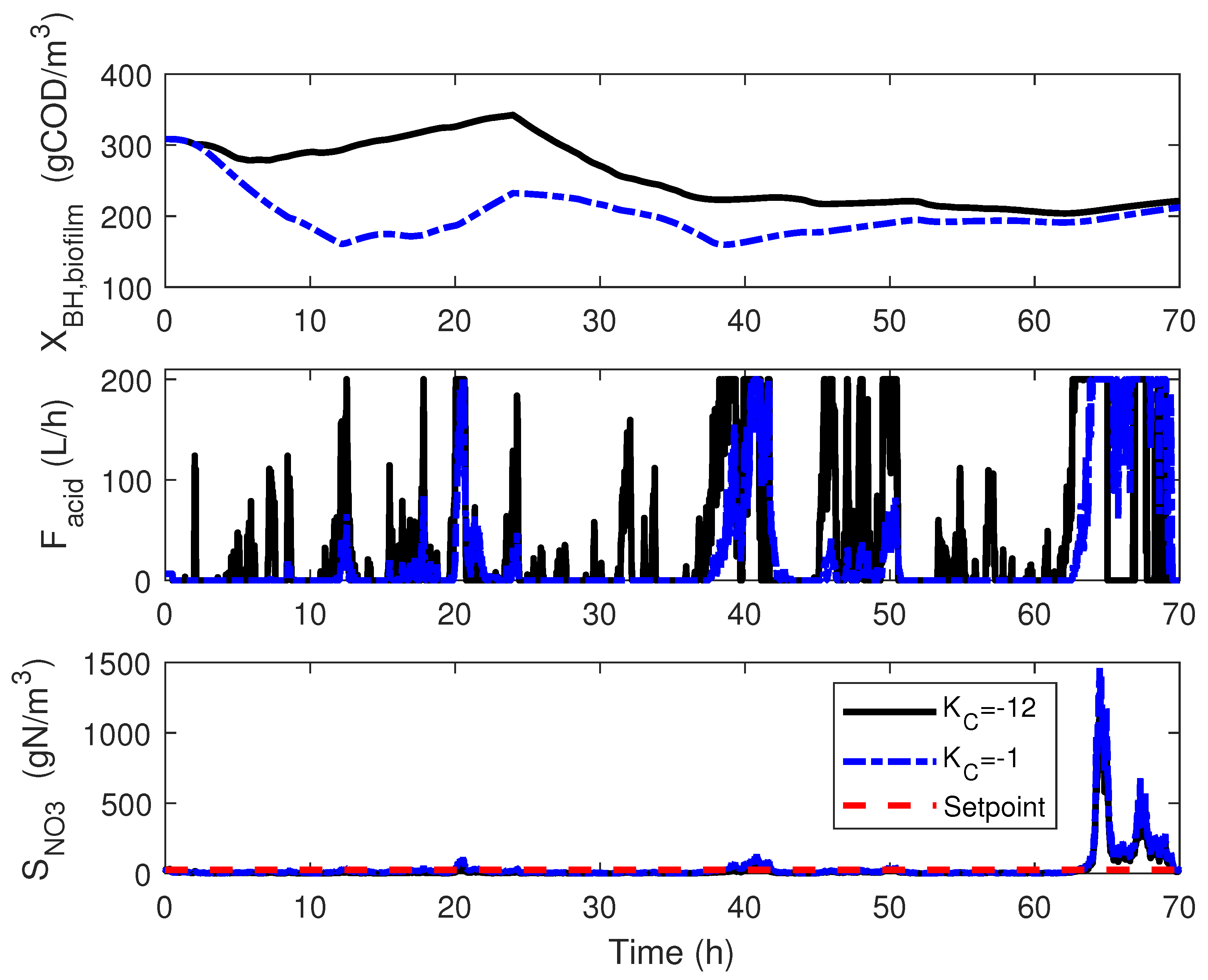
3. Control Implementation: Classical Approach

This section aims at first designing a classical PID controller to regulate the nitrate level in the denitrification reactor. From the corresponding model of differential Equations (3) and (4), acetic acid is obviously the sole manipulated variable and the following control law is proposed:
F A c i d ( t ) = F A c i d ¯ + K C e ( t ) + 1 τ I 0 t e ( t * ) d t * + τ D d e ( t ) d t
e ( t ) = S N O 3 * S N O 3 ( t )
where F A c i d ¯ represents the initial acetic acid flowrate ensuring the industrial plant nominal steady-state ( F A c i d ¯ = 6.4 L/h), e ( t ) represents the measurement error, K C is the proportional gain, τ I and τ D , respectively, are the integral and derivative time constants, S N O 3 * is the desired nitrate concentration setpoint and S N O 3 ( t ) is the measured nitrate concentration. Expression (13) therefore aims at compensating any deviation from the chosen nominal steady-state trajectory which is assumed to be a priori knowledge from heuristics. Although (13) only presents three parameters, finding optimal settings without resorting to a systematic procedure may be complex. One way to design the gains is to first focus on the Proportional-Integral (PI) (i.e., τ D = 0 ) part in order to set a satisfactory steady-state response (no steady-state error) and then consider the derivative part to improve the transient response [13,23].
In this study, the SIMC design method, as presented in [13], is chosen since it involves the transfer function of the system which can be easily computed considering a specific operating point and the corresponding step response, for instance, using the MATLAB model identification toolbox.
As shown in Figure 3, a one pole model already provides a very good approximation, and reads:
G ( s ) = k e θ s τ 1 s + 1 = 32 8.9 × 10 2 s + 1
The numerator of (15) shows that the system presents a steady-state gain ( G ( 0 ) ) equal to 32 and no delay ( θ = 0 ) while the denominator provides the system time constant ( τ 1 ) which, as expected, is particularly large (890 h). Such slow systems, according to [13], may be approximated by a simple integrator:
k e θ s τ 1 s + 1 k e θ s s
using the ratio between the gain G ( 0 ) and the time constant τ 1 , denominated k , to determine PI-settings in a much shorter time frame (see Figure 4). k is therefore calculated as follows:
k = Δ y Δ t Δ u = 22.09 25.59 ( 240 24 ) ( 6.762 6.44 ) = 0.05
where Δ y represents the variation in nitrate concentration during Δ t hours, for a variation in acid flowrate Δ u .
The SIMC method then proposes, for a general first-order process with delay, the PID tuning rules presented in Table 2, where τ C represents the time constant of the desired first-order response of the system. The second row shows how this method is applied to the considered industrial-scale plant.
Considering y, the current nitrate concentration in the denitrification filter, y S the desired setpoint, and θ the time delay, Equation (18) shows the relation between these variables and τ C :
Y ( s ) Y s ( s ) d e s i r e d = 1 τ C s + 1 e θ s
The rate at which nitrate is produced/consumed in the system depends on either the quantity of ammonia released by fish (and consequent quantity converted into nitrate) or the amount of nitrate the denitrification biofilter is able to convert into nitrogen (gas). Regarding nitrate consumption, an increase in available carbon source induces biomass growth and nitrate consumption increases (assuming that the biofilter size is properly designed). However, nitrate production is entirely driven by the quantity of ammonia produced in the system. τ C is then limited by the “maximum” production rate of nitrate and can be estimated using the quantity of ammonia produced by the fish. This can be further explained by Equation (18), considering θ = 0 , represented in Figure 5. It has to be noticed that τ C should always be greater than d y y s d t m a x , that is, τ C τ C , m i n as shown in Figure 5, depending on the amount of ammonia excreted by fish.
The controller parameter calculation conditions, related to the case-study, are presented in Table 3. All the ammonia introduced in the system is considered as completely converted into nitrate.
As shown in Figure 6, where setpoint changes of +15/−15 gN/m3 are simulated, an anti-windup configuration (using Equation (19)) is recommended to avoid detrimental effects due to input saturation and the control law reads:
F A c i d ( t ) = F A c i d ¯ + K C e ( t ) + 1 τ I 0 t ( e ( t * ) e a w ) d t * e ( t ) = S N O 3 * S N O 3 ( t )
with e a w being the anti-windup term calculated by the following equation:
e a w = K a w ( F a c i d , t F a c i d , m a x ) i f F a c i d , t > F a c i d , m a x K a w ( F a c i d , t F a c i d , m i n ) i f F a c i d , t < F a c i d , m i n 0 F a c i d , m i n < F a c i d , t < F a c i d , m a x
e a w is only greater than 0 when the controller output is greater than the allowed maximum value ( F a c i d , m a x = 200 L/h) or lower than its minimum value ( F a c i d , m i n = 0 L/h). When this happens, the control action is limited and e a w is calculated accordingly ( K a w is the anti-windup gain). Figure 6 shows the effect of the anti-windup when a K a w value of −1 is used. When the nitrate setpoint is increased, the controller decreases the acid flowrate accordingly. However, nitrate concentration will continue to increase due to the ammonia conversion reaction which causes the integral term of the PI controller to go on increasing. When the nitrate concentration finally reaches the desired setpoint, the accumulated integral action entails overshoot. K a w values chosen between −0.1 and −10 are sufficient to solve the issue. Nevertheless, using a high K a w value tends to slow down setpoint tracking. A K a w value of 1 is ideally chosen and used in future simulations.
The design of the derivative gain is achieved following the analysis of the controller response to setpoint changes. Comparative results using different derivative gain values (driven by the choice of τ D ) can be found in Figure 7. The input calculated by the PID therefore reads:
F A c i d = F A c i d ¯ + K C e ( t ) + 1 τ I 0 t ( e ( t * ) e a w ) d t * + τ D ( e ( t ) η )
η ˙ = ( e ( t ) η ) τ D
where the derivative term is approximated by a continuous high-pass filter using η as intermediate variable. Including the derivative action leads to the new results of Figure 7, where oscillations are attenuated and the tracking is improved. A τ D value of 1 provides the most satisfactory result and is therefore selected.
The resulting PID performance is assessed in Figure 8 where, following several setpoint changes and step disturbances in waste production ( ϑ S N H ), robust and fast tracking is achieved. Values of 11.6 L·m3/(g·h), 6.9 h, 1 h and 1 are, respectively, used for K C , τ I , τ D and K a w . Robustness analysis with respect to other operating condition disturbances is also presented in Figure 9. Variations in the available biomass concentration X B H and the bypass flowrate F d e n i t r i are identified as severe system disturbances. A sudden increase in biomass decay rate ( b H term in Table S2 is increased 3 fold, from 2.6 × 10 2 to 7.8 × 10 2 h−1) is therefore simulated and indeed causes response oscillations, as shown in Figure 9, while step variations on the bypass flowrate are compensated very fast.
For the exact same perturbation in the biomass decay rate as in the previous test, the situation gets worse when adding measurement noise, as shown in Figure 10, where a Gaussian noise with zero mean and 10 % relative standard deviation is added to the measured variable ( S N O 3 ). A sampling time of 0.01 h is also used to match the probe measurement sampling process. The controller obviously faces tracking problems, sometimes reaching unacceptable nitrate concentration values even when trying to retune the controller proportional gain (Figure 10 shows the results for two values of the gain). To avoid this undesired effect, two solutions could be considered—they are, (a) low-pass filtering of the output signal or (b) replacing the PID by a PI, which is, in essence, less sensitive to measurement noise.

4. Linearizing Control

A linearizing control strategy, as illustrated in Figure 11, may also be proposed as an alternative solution.
The control law is established based on a simplified ASM1 model [19] (in order to limit the quantity of measured variables) and the following assumptions:
  • Only the denitrification reactor is considered;
  • This reactor only contains heterotrophic bacteria;
  • Since the oxygen concentration is low, no nitrification can occur;
  • Biomass is retained in the tank ( X B H , o u t = 0 ) ;
  • Only three other components besides biomass are considered: oxygen ( S O ), easily biodegradable organic matter ( S S ) and nitrate ( S N O 3 );
  • Only two reactions are assumed to occur:
    • Aerobic growth of heterotrophs:
      S S + S O X B H ;
    • Anoxic growth of heterotrophs on nitrate:
      S S + S N O 3 X B H ;
  • Acid is added as a carbon source and φ represents the conversion of acid flowrate ( F a c i d , L / h ) into easily biodegradable carbon source flowrate ( g C O D / h ) ).
Applying mass balances to (23) and (24), the following simplified differential equation system is obtained:
d S S d t = F D e n i t r i V D e n i t r i S S , i n ( F D e n i t r i + F a c i d ) V D e n i t r i S S + ϕ S S + F a c i d φ V D e n i t r i
d S N O 3 d t = F D e n i t r i V D e n i t r i S N O 3 , i n ( F D e n i t r i + F a c i d ) V D e n i t r i S N O 3 + ϕ N O 3
where ϕ S S and ϕ N O 3 are the easily biodegradable organic matter and nitrate reaction rates given by:
ϕ S S = υ S S , a e r o b ρ 1 + υ S S , a n o x ρ 2
ϕ N O 3 = υ N O 3 ρ 2
where υ S S , a e r o b , υ S S , a n o x and υ N O 3 are stoichiometric coefficients depending on biomass yield Y H as in:
υ S S , a e r o b = υ S S , a n o x = υ S S = 1 Y H
υ N O 3 = 1 Y H 2.86 Y H
and ρ 1 and ρ 2 are the aerobic and anoxic growth rates of heterotrophs:
ρ 1 = μ H S O S O + K O H S S S S + K S X B H
ρ 2 = η g μ H S S S S + K S K O H S O + K O H S N O 3 S N O 3 + K N O X B H
Considering a first-order linear reference as in (33):
d S N O 3 d t = λ l i n ( S N O 3 * S N O 3 )
where S N O 3 * is the desired nitrate concentration setpoint. Replacing Equation (33) in Equation (26):
ρ 2 = 2.86 Y H 1 Y H F D e n i t r i V D e n i t r i ( S N O 3 , i n S N O 3 ) F a c i d V D e n i t r i S N O 3 λ l i n ( S N O 3 * S N O 3 )
In steady-state, S S variation tends to zero:
d S S d t 0
and injecting (34) into (25), assuming (35), yields:
F a c i d V D e n i t r i S S F a c i d V D e n i t r i φ = F D e n i t r i V D e n i t r i ( S S , i n S S ) 1 Y H ρ 1 2.86 1 Y H F D e n i t r i V D e n i t r i ( S N O 3 , i n S N O 3 ) F a c i d V D e n i t r i S N O 3 λ l i n ( S N O 3 * S N O 3 )
F a c i d S S 2.86 1 Y H S N O 3 φ V D e n i t r i = F D e n i t r i V D e n i t r i S S , i n S S 2.86 1 Y H ( S N O 3 , i n S N O 3 ) 1 Y H ρ 1 + 2.86 1 Y H λ l i n ( S N O 3 * S N O 3 )
F a c i d = F D e n i t r i V D e n i t r i S S , i n S S 2.86 1 Y H ( S N O 3 , i n S N O 3 ) S S 2.86 1 Y H S N O 3 φ V D e n i t r i 1 Y H ρ 1 + 2.86 1 Y H λ l i n ( S N O 3 * S N O 3 ) S S 2.86 1 Y H S N O 3 φ V D e n i t r i
As previously mentioned, an anti-windup term should be added to cancel input saturation effects:
F a c i d = F D e n i t r i ( S N O 3 , i n S N O 3 + 1 2.86 S O , i n ) 1 Y H ρ 1 + λ l i n ( S N O 3 * S N O 3 ) 1 Y H 2.86 φ + S N O 3 λ l i n , I ( S N O 3 * S N O 3 + e a w , l i n ) 1 Y H 2.86 φ + S N O 3
e a w , l i n = K a w , l i n ( F a c i d F a c i d , m a x ) i f F a c i d > F a c i d , m a x K a w , l i n ( F a c i d F a c i d , m i n ) i f F a c i d < F a c i d , m i n 0 F a c i d , m i n < F a c i d < F a c i d , m a x
As shown in Figure 12, the linearizing controller provides good performances even in the presence of measurement noise with zero mean and 10 % relative standard deviation, and biomass concentration decrease. However, in an attempt to decrease the undesired oscillations, two additional strategies, which aim at being more robust to model uncertainties, are proposed in the following section, one combining both control structures in cascade and another estimating the biomass unknown dynamics.

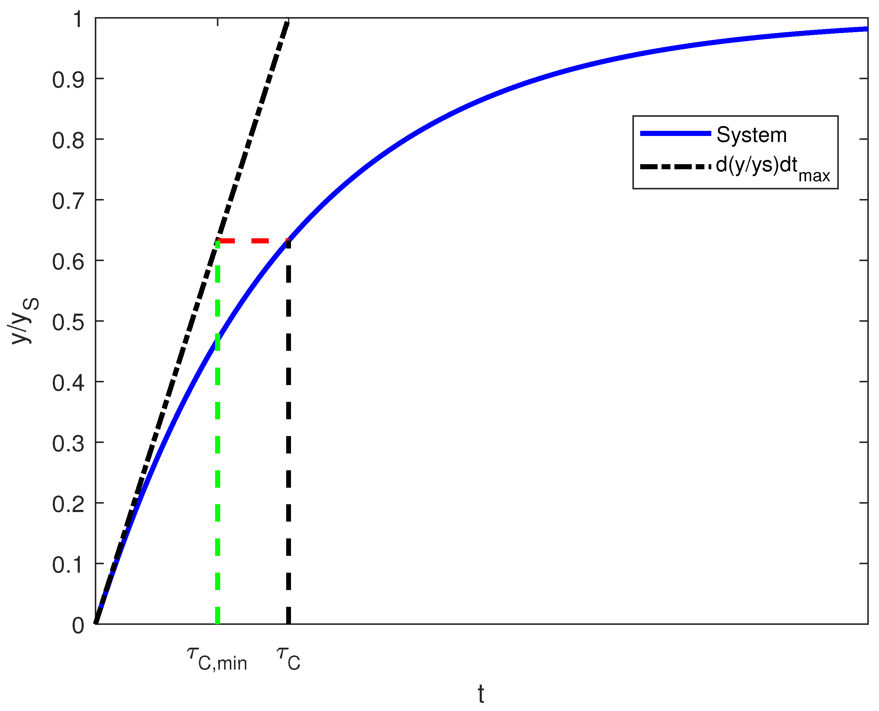
4.1. Cascade Control

The cascade control methodology takes advantage of linearizing control to impose a first-order closed-loop dynamic in the inner loop, and a PI controller is used in the outer loop (see Figure 13). This cascade structure provides robustification, for instance, to model uncertainties, as follows:
F a c i d = F D e n i t r i ( S N O 3 , i n S N O 3 + 1 2.86 S O , i n ) 1 Y H ρ L i n + λ l i n ( S N O 3 * S N O 3 ) 1 Y H 2.86 φ + S N O 3
ρ 1 = μ H S O , b S O + K O H S S S S + K S X B H
where
S N O 3 * ( t ) = S N O 3 * ¯ + K C , c a s c a d e e ( t ) + 1 τ I , c a s c a d e 0 t e ( t * ) d t *
e ( t ) = S N O 3 * ( t ) S N O 3 ( t )

4.2. Adaptive Linearizing Control

Lumping the kinetic uncertainties into one single parameter θ ^ , Equation (38) can be re-written:
F a c i d = F D e n i t r i ( S N O 3 , i n S N O 3 + 1 2.86 S O , i n ) + θ ^ + λ l i n ( S N O 3 * S N O 3 ) 1 Y H 2.86 φ + S N O 3
with
θ = 1 Y H ρ 1
θ ˜ = θ θ ^
where θ ˜ represents parameter mismatch θ ˜ = θ θ ^ . An adaptive scheme, as described in [16,24], can be designed to develop an asymptotically stable control law, considering the following positive Lyapunov candidate function:
V L ( t ) = 1 2 S ˜ N O 3 2 + θ ˜ 2 γ
and its time derivative:
V L ˙ = d S ˜ N O 3 d t S ˜ N O 3 + θ ˜ d θ ˜ d t 1 γ
where S ˜ N O 3 = S N O 3 * S N O 3 , θ ˜ = θ θ ^ and γ is a striclty positive parameter. All the terms in ρ L i n are assumed to be slowly varying so that d θ d t = 0 and we get:
d θ ˜ d t = d θ ^ d t
Considering possible parameter mismatch, the error dynamics may be written:
d S ˜ N O 3 d t = λ S ˜ N O 3 θ ˜
Replacing Equations (50) and (51) in (49), we obtain:
V L ˙ = λ S ˜ N O 3 2 θ ˜ S ˜ N O 3 θ ˜ d θ ^ d t 1 γ
Considering Lyapunov stability theory, V L ˙ should be negative and since the first term of (52) is, as long as the second and third terms cancel each other, the stability of the closed-loop is verified, as in:
θ ˜ S ˜ N O 3 θ ˜ d θ ^ d t 1 γ = 0
d θ ^ d t = S ˜ N O 3 γ
The adaptive control law reads:
F a c i d = F D e n i t r i ( S N O 3 , i n S N O 3 + 1 2.86 S O , i n ) + θ ^ + λ l i n ( S N O 3 * S N O 3 ) 1 Y H 2.86 φ + S N O 3
with
d θ ^ d t = S ˜ N O 3 γ
It should be noticed that the adaptive linearizing controller is equivalent to (38) where an integral action is added.

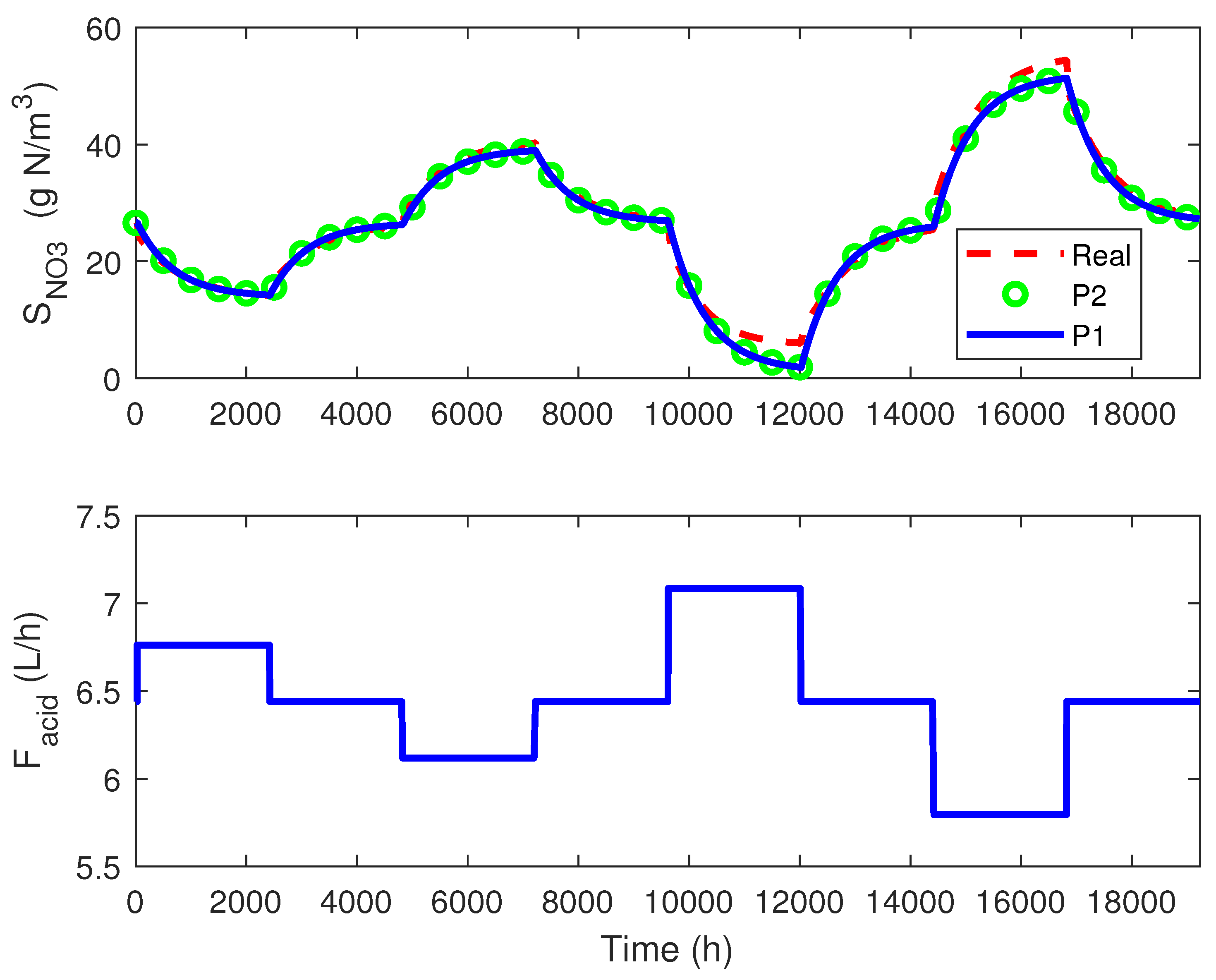
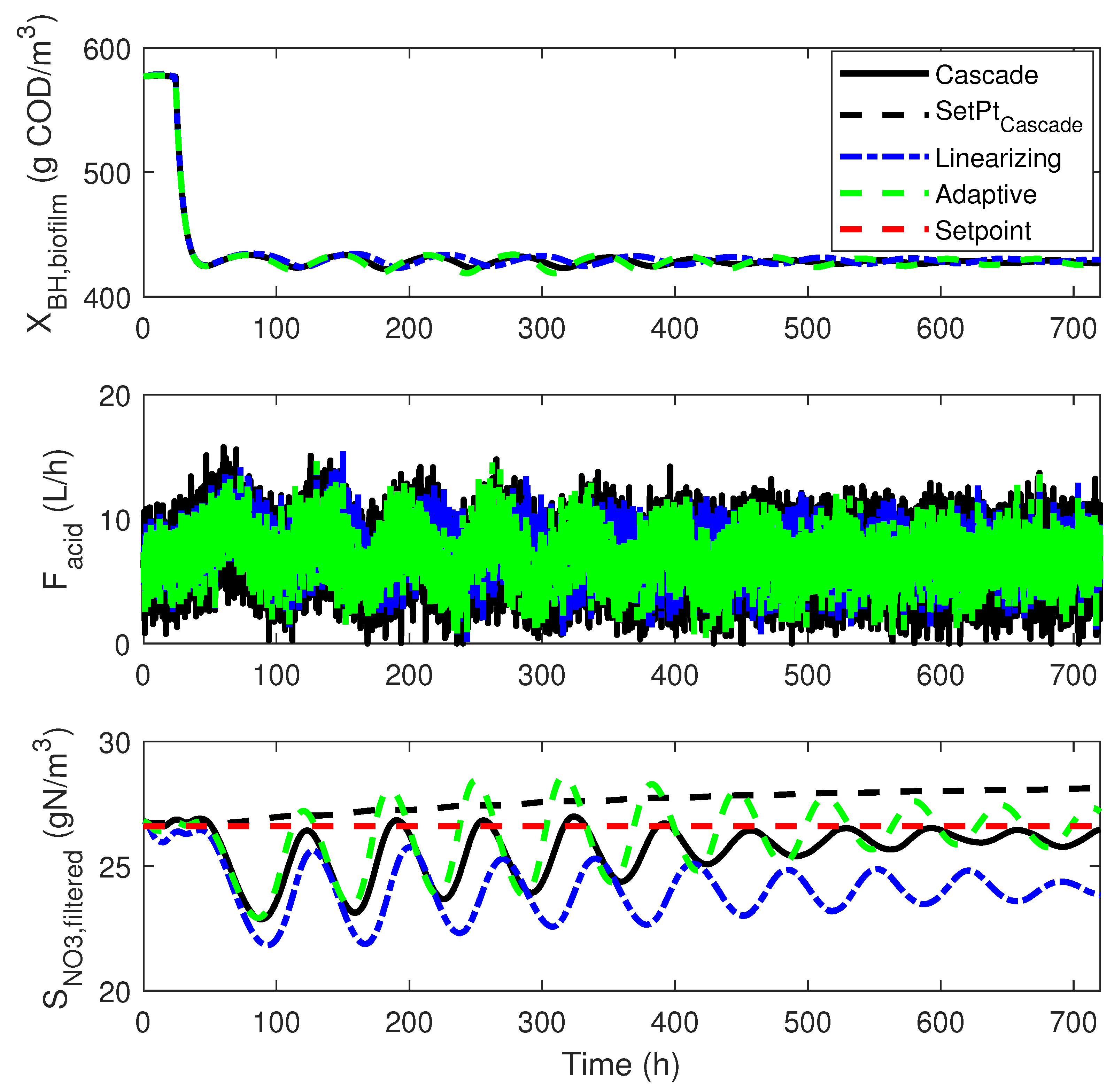
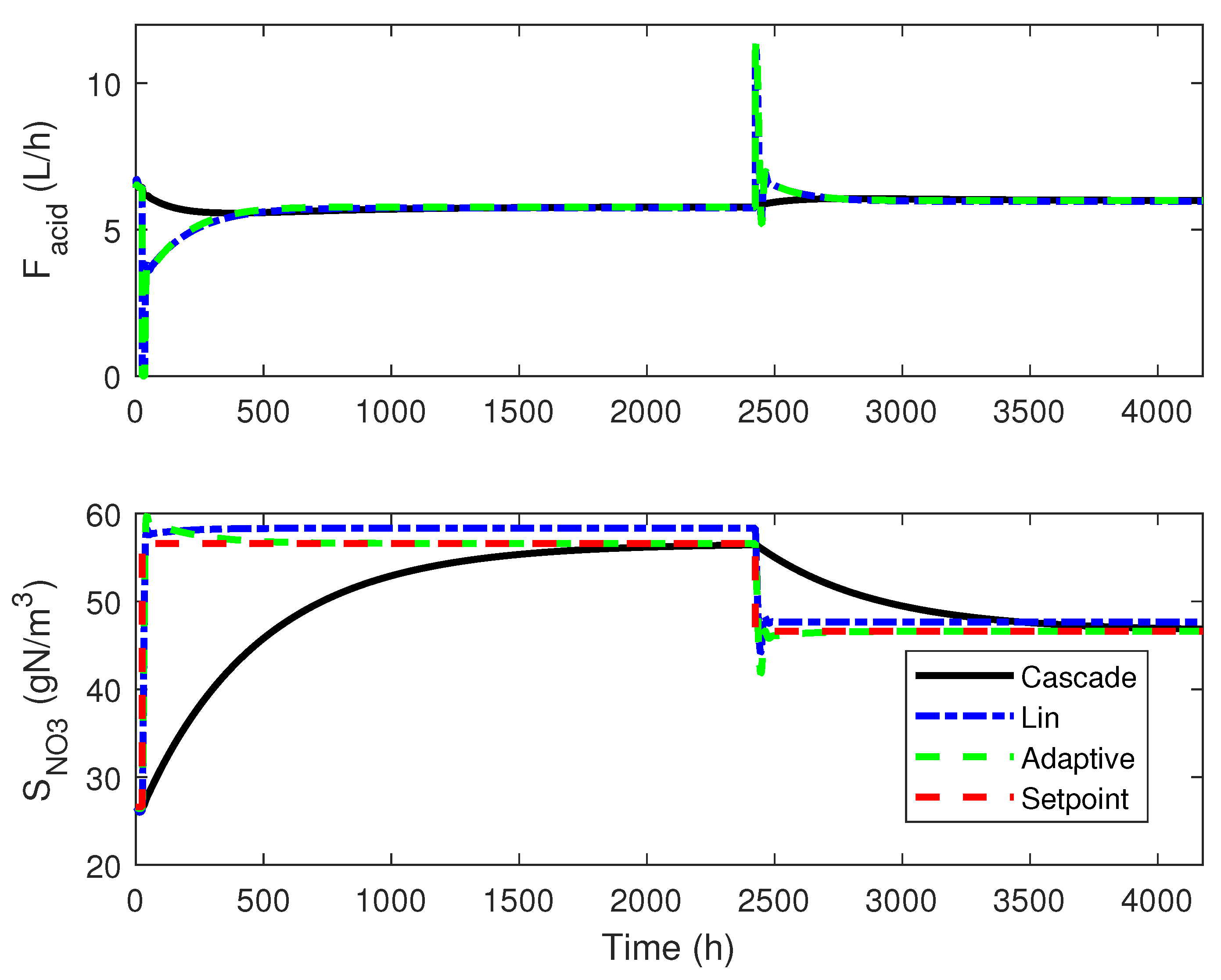
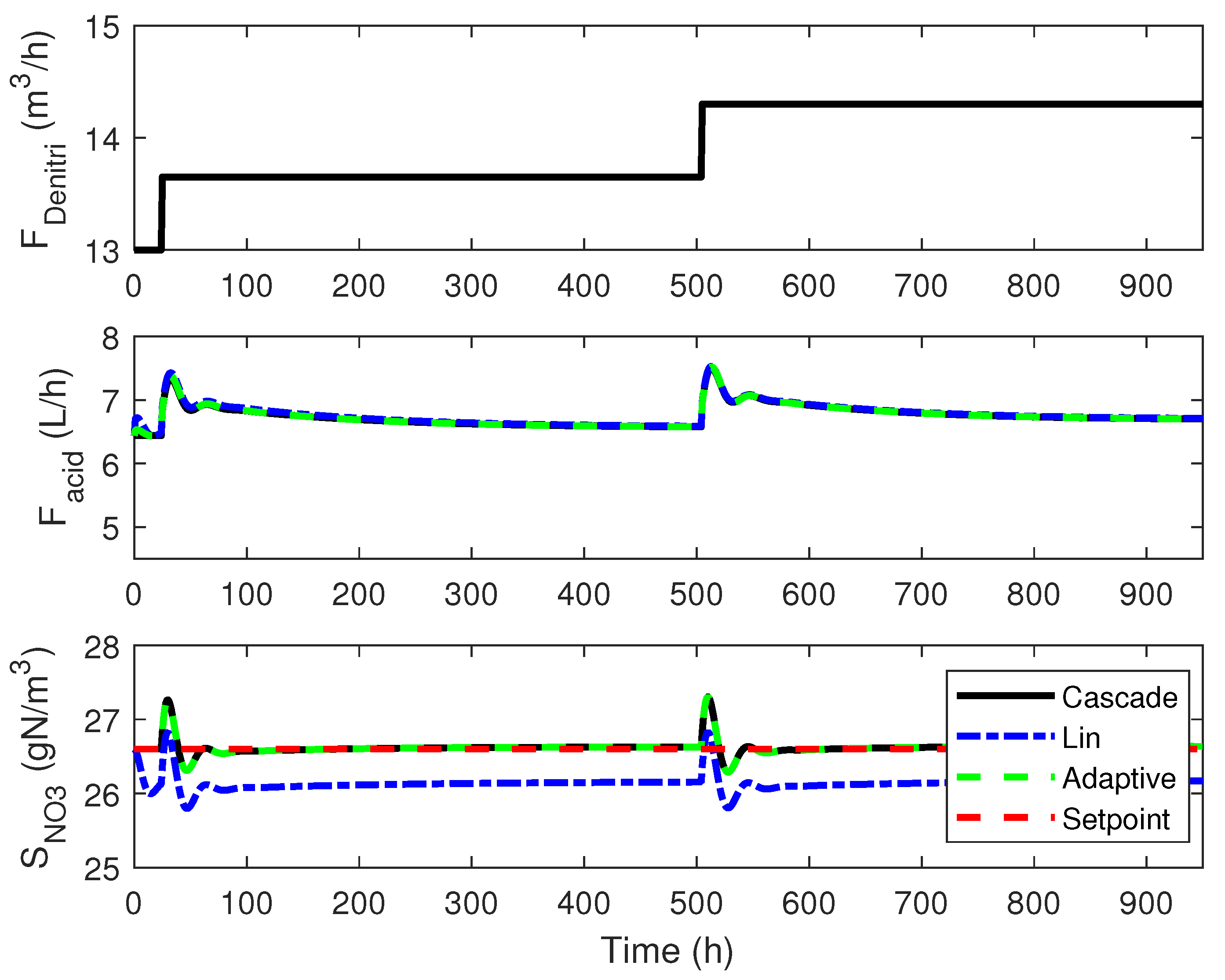
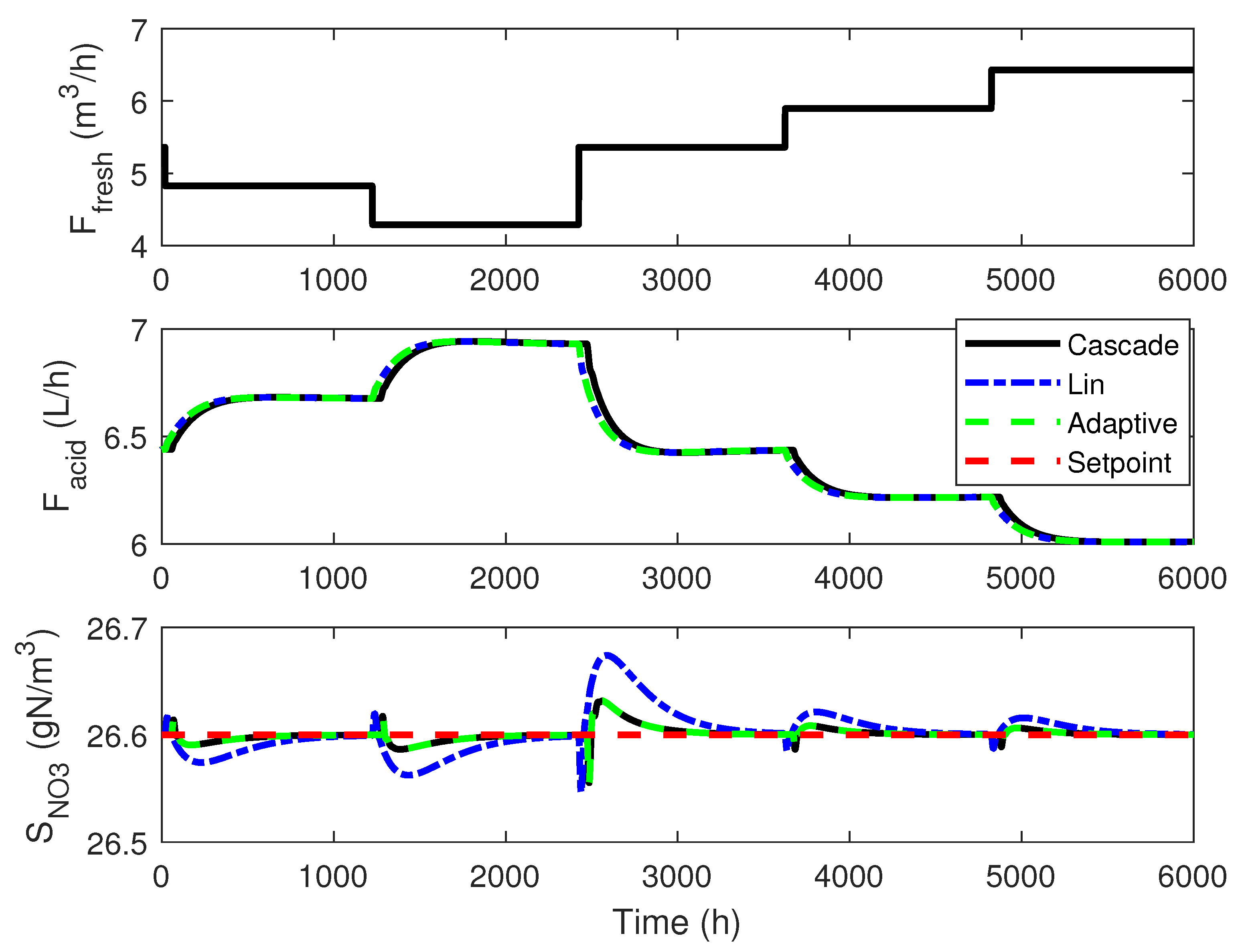
4.3. Numerical Results

Simulation results aim at assessing the controller performance following an increase in biomass (death rate) considering measurement white noise with zero mean and 10 % standard deviation on all measured variables ( S N O 3 , S S , S O and X B H ), as shown in Figure 12. A sampling time of 0.01 h is used to simulate the corresponding probe behavior. Regarding the linearizing controller, the parameters 0.5 h−1, 6 L/h2 m3 and 10 are, respectively, used for λ l i n , λ l i n , I and K a w , l i n . The PI used in cascade is parameterized with K C , c a s c a d e = 0.001 and τ I , c a s c a d e = 0.5 h (keeping λ l i n = 0.5 h−1) and the adaptive controller uses γ = 5 (keeping λ l i n = 0.5 h−1). All the controllers perform reasonably well when noise is added and both the adaptive and cascade controllers are capable of attenuating the previously described oscillations.
In addition, comparative results between the linearizing controller with the cascade and the adaptive controller for several system disturbances are shown in Figure 14, Figure 15, Figure 16 and Figure 17.
It is noticeable from Figure 9 (left) and Figure 12 that all controllers oscillate following a perturbation in the biomass concentration. This is related to the operating point of the RAS and, by setting a new higher nitrate setpoint, it is possible to obtain a smoother response, as shown in Figure 18.

5. Conclusions and Perspectives

In this study, a control study of a recirculation aquaculture system is undertaken. Different control methodologies are tested in simulations for an industrial scale system. Both PID and linearizing controllers are capable of keeping the system stable when used with an anti-windup action. The PID controller gains can be calculated based on fish waste production (ammonia). The addition of a derivative action leads to a noticeable decrease in controller output oscillations. Nonetheless, the PID presents robustness issues when considering measurement noise. The linearizing controller is, however, able to overcome this problem and can also be further improved by adding an adaptive law to face possible model uncertainties. A cascade control strategy (combining PI and linearizing controllers) may also improve the control robustness to model uncertainties, compromising the tracking performance. The system has an operational region around which all the considered feedback strategies present oscillating responses. Operational conditions should then be changed to accommodate this phenomenon. The controllers show good robustness with respect to disturbances, such as the increase in ammonia production due to variations in the fish population. The control strategies discussed in this article are versatile and could be applied to other RAS configurations at different scales. Future perspectives could include the analysis of nitrite accumulation and the possibility to limit its concentration.

Supplementary Materials

The following are available online at https://www.mdpi.com/2227-9717/8/10/1306/s1, Table S1: Stoichiometry for carbon oxidation, nitrification, and denitrification; Table S2: Process kinetics for carbon oxidation, nitrication, and denitrication.

Author Contributions

Conceptualization: A.V.W.; methodology: L.D.; computer implementation: P.A.; numerical study: P.A. and L.D.; writing—original draft preparation: P.A. and L.D.; writing—review and editing: A.V.W.; supervision: L.D. and A.V.W. All authors have read and agreed to the published version of the manuscript.

Funding

The authors gratefully acknowledge the support of the WAGRALIM project NUTRIVERT funded by the Walloon Region.

Conflicts of Interest

The authors declare no conflict of interest.

References

  1. FAO. The State of World Fisheries and Aquaculture 2018: Meeting the Sustainable Development Goals; Food and Agriculture Organization of the United Nations: Rome, Italy, 2018; ISBN 9789251305621. [Google Scholar]
  2. Ruiz, P.; Vidal, J.M.; Sepúlveda, D.; Torres, C.; Villouta, G.; Carrasco, C.; Aguilera, F.; Ruiz-Tagle, N.; Urrutia, H. Overview and future perspectives of nitrifying bacteria on biofilters for recirculating aquaculture systems. Rev. Aquac. 2019, 12, 1478–1494. [Google Scholar] [CrossRef]
  3. Bregnballe, J. A Guide to Recirculation Aquaculture: An Introduction to the New Environmentally Friendly and Highly Productive Closed Fish Farming Systems; Food and Agriculture Organization of the United Nations: Copenhagen, Denmark, 2015. [Google Scholar]
  4. Gutierrez-Wing, M.T.; Malone, R.F. Biological filters in aquaculture: Trends and research directions for freshwater and marine applications. Aquac. Eng. 2006, 34, 163–171. [Google Scholar] [CrossRef]
  5. Pungrasmi, W.; Phinitthanaphak, P.; Powtongsook, S. Nitrogen removal from a recirculating aquaculture system using a pumice bottom substrate nitrification-denitrification tank. Ecol. Eng. 2016, 95, 357–363. [Google Scholar] [CrossRef]
  6. Wik, T.E.; Lindén, B.T.; Wramner, P.I. Integrated dynamic aquaculture and wastewater treatment modelling for recirculating aquaculture systems. Aquaculture 2009, 287, 361–370. [Google Scholar] [CrossRef] [Green Version]
  7. Liu, X.; Wang, H.; Yang, Q.; Li, J.; Zhang, Y.; Peng, Y. Online control of biofilm and reducing carbon dosage in denitrifying biofilter: Pilot and full-scale application. Front. Environ. Sci. Eng. 2017, 11, 4. [Google Scholar] [CrossRef]
  8. Du, R.; Peng, Y.; Cao, S.; Li, B.; Wang, S.; Niu, M. Mechanisms and microbial structure of partial denitrification with high nitrite accumulation. Appl. Microbiol. Biotechnol. 2015, 4, 2011–2021. [Google Scholar]
  9. Lee, P.G.; Lea, R.N.; Dohmann, E.; Prebilsky, W.; Turk, P.E.; Ying, H.; Whitson, J.L. Denitrification in aquaculture systems: An example of a fuzzy logic control problem. Aquac. Eng. 2000, 23, 37–59. [Google Scholar] [CrossRef]
  10. Join, C.; Bernier, J.; Mottelet, S.; Fliess, M.; Rechdaoui-Guérin, S.; Azimi, S.; Rocher, V. A simple and efficient feedback control strategy for wastewater denitrification. IFAC-PapersOnLine 2017, 50, 7657–7662. [Google Scholar] [CrossRef]
  11. Zúñiga, I.T.; Queinnec, I.; Vande Wouwer, A. Observer-based output feedback linearizing control strategy for a nitrification–denitrification biofilter. Chem. Eng. J. 2012, 191, 243–255. [Google Scholar] [CrossRef]
  12. Wahab, N.A.; Katebi, R.; Balderud, J. Multivariable PID control design for activated sludge process with nitrification and denitrification. Biochem. Eng. J. 2009, 45, 239–248. [Google Scholar] [CrossRef]
  13. Skogestad, S.; Grimholt, C. The SIMC method for smooth PID controller tuning. In PID Control in the Third Millennium; Springer: London, UK, 2012; pp. 147–175. [Google Scholar]
  14. Seborg, D.E. Process Dynamics and Control, 2nd ed.; John Wiley & Sons, Inc.: Hoboken, NJ, USA, 2003. [Google Scholar]
  15. Dochain, D. Bioprocess Control; John Wiley & Sons, Ltd.: Hoboken, NJ, USA, 2008. [Google Scholar]
  16. Dewasme, L.; Coutinho, D.; Vande Wouwer, A. Adaptive and Robust Linearizing Control Strategies for Fed-Batch Cultures of Microorganisms Exhibiting Overflow Metabolism. In Informatics in Control, Automation and Robotics; Cetto, J.A., Ferrier, J.L., Filipe, J., Eds.; Springer Berlin Heidelberg: Berlin/Heidelberg, Germany, 2011; pp. 283–305. [Google Scholar]
  17. Tebbani, S.; Lopes, F.; Celis, G.B. Nonlinear control of continuous cultures of Porphyridium purpureum in a photobioreactor. Chem. Eng. Sci. 2015, 123, 207–219. [Google Scholar] [CrossRef]
  18. Aguilar-López, R. Input-Output Linearizing-type controller design with application to continuous bioreactor. Comptes Rendus de l’Académie Bulgare des Sciences: Sciences Mathématiques et Naturelles 2016, 70. [Google Scholar]
  19. Henze, M.; Gujer, W.; Mino, T.; van Loosdrecht, M. Activated Sludge Models ASM1, ASM2, ASM2D and ASM3 (Scientific & Technical Reports, No. 9); IWA Publishing: London, UK, 2000. [Google Scholar]
  20. Thomas, S.L.; Piedrahita, R.H. Oxygen consumption rates of white sturgeon under commercial culture conditions. Aquac. Eng. 1997, 16, 227–237. [Google Scholar] [CrossRef]
  21. Szczepkowski, M.; Szczepkowska, B.; Kolman, R. Comparison of oxygen consumption and ammonia excretion by siberian sturgeon (acipenser baeri drandt) and its hybrid with green sturgeon (acipenser medirostris ayres). Arch. Ryb. Pol. 2000, 8, 205–211. [Google Scholar]
  22. Copp, J.B. The COST Simulation Benchmark: Description and Simulator Manual. COST Action 624 and COST Action 682; Office for Official Publications od the European Union: Luxembourg, 2002. [Google Scholar]
  23. Phillips, C.L.; Harbor, R.D. Feedback Control Systems, 4th ed.; Prentice-Hall, Inc.: Upper Saddle River, NJ, USA, 2000. [Google Scholar]
  24. Bastin, G.; Dochain, D. On-line estimation and adaptive control of bioreactors. Anal. Chim. Acta 1991, 243, 324. [Google Scholar] [CrossRef]
Figure 1. Industrial scale RAS.
Processes 08 01306 g001
Figure 2. Simulated response of the industrial scale RAS to a step increase in an inert soluble component production rate by 1 gCOD/(m3·h). First order model presented for comparison purpose.
Processes 08 01306 g002
Figure 3. S N O 3 response following several step variations in acid flowrate.
Processes 08 01306 g003
Figure 4. S N O 3 evolution following a step increase in acid flowrate.
Processes 08 01306 g004
Figure 5. Variation of ( y y s ) as a function of the time constant.
Processes 08 01306 g005
Figure 6. Application of the PI controller with and without anti-windup following a nitrate setpoint variation. A K a w value of −1 is used.
Processes 08 01306 g006
Figure 7. Selection of the PID derivative gain τ D .
Processes 08 01306 g007
Figure 8. Closed-loop system input/output evolution following (left) several setpoint changes and (right) 5 to 10 % step variations in waste production ( ϑ N H ).
Processes 08 01306 g008
Figure 9. Closed-loop system input/output evolutions following (left) an increase in biomass decay rate from 2.6 × 10 2 to 7.8 × 10 2 h−1 and (right) 5 to 10 % step variations applied to the bypass flowrate ( F D e n i t r i ).
Processes 08 01306 g009
Figure 10. Nitrate concentration and acid flowrate evolutions for an increase in biomass decay rate from 2.6 × 10 2 to 7.8 × 10 2 h 1 while using two PID controllers with different proportional gains ( K C )—Gaussian noise with zero mean and 10 % relative standard deviation is added to the measured variable ( S N O 3 ).
Processes 08 01306 g010
Figure 11. Linearizing control scheme.
Processes 08 01306 g011
Figure 12. Simulation results obtained for the linearizing, adaptive and cascade controllers when the biomass death rate is increased and a 10% measurement noise on all measured variables ( S N O 3 , S S , S O and X B H ) is added. S e t P t C a s c a d e represents the corrected setpoint curve and S e t p o i n t the desired setpoint.
Processes 08 01306 g012
Figure 13. Linearizing controller and PI in cascade.
Processes 08 01306 g013
Figure 14. Nitrate concentration and acid flowrate evolutions for a setpoint step variation using different controllers: cascade ( C a s c a d e ), classical linearizing ( L i n ) and adaptive linearizing controllers ( A d a p t i v e ).
Processes 08 01306 g014
Figure 15. Nitrate concentration and acid flowrate evolutions for 5 to 10 % variations in ammonia (waste) production ( ϑ S N H ) using different controllers: cascade ( C a s c a d e ), classical linearizing ( L i n ) and adaptative linearizing controllers ( A d a p t i v e ).
Processes 08 01306 g015
Figure 16. Nitrate concentration and acid flowrate evolutions for 5 to 10 % variations in bypass flowrate ( F D e n i t r i ) using different controllers: cascade ( C a s c a d e ), classical linearizing ( L i n ) and adaptative linearizing controllers ( A d a p t i v e ).
Processes 08 01306 g016
Figure 17. Nitrate concentration and acid flowrate evolutions for 5 to 10 % variations in fresh water flowrate ( F f r e s h ) using different controllers: cascade ( C a s c a d e ), classical linearizing ( L i n ) and adaptative linearizing controllers ( A d a p t i v e ).
Processes 08 01306 g017
Figure 18. Simulation results obtained for the linearizing, adaptive and cascade controllers when the biomass death rate is increased and a 10% measurement noise on all measured variables ( S N O 3 , S S , S O and X B H ) is added and when a higher steady-state nitrate concentration and setpoint are considered. S e t P t C a s c a d e represents the corrected setpoint curve and S e t p o i n t is the desired setpoint.
Processes 08 01306 g018
Table 1. Fish waste production rates.
CorrespondingDescription ϑ waste Units
component ξ
S I Inert soluble organic material994gCOD/h
S S Readily biodegradable organic material0gCOD/h
X I Inert particulate organic material994gCOD/h
X S Slowly biodegradable substrate 1.2 × 10 4 gCOD/h
X B H Active heterotrophic biomass0gCOD/h
X N S Active ammonia oxidizing bacteria0gCOD/h
X N B Active nitrite oxidizing bacteria0gCOD/h
X P Part. products from biomass decay 4.0 × 10 3 gCOD/h
S 0 Dissolved oxygen 6.1 × 10 3 agCOD/h
S N O 3 Nitrate nitrogen0gN/h
S N H Ammonium and ammonia nitrogen1.5 × 10 3 gN/h
S N D Soluble biodegradable organic nitrogen355gN/h
X N D Particulate biodegradable organic nitrogen355gN/h
S A l k Alkalinity (as HCO3 equivalents)0gCOD/h
S C O 2 Dissolved carbon dioxide8.4 × 10 3 gCO2/h
S P Phosphorus497gP/h
S N O 2 Nitrite concentration0gN/h
a Negative since fish consume oxygen rather than expel it.
Table 2. PI parameter calculation using the SIMC method.
Process G ( s ) K C τ I τ D
SIMC PID settingsFirst-order k e θ s s 1 k 1 τ C + θ m i n { 4 ( τ C + θ ) } -
Industrial-scale plant modelFirst-order k = 0.05 τ 1 = 8.9 × 10 2 θ = 0 1 0.05 1 τ C m i n { 4 τ C } -
Table 3. Parameter values for the industrial case-study controller.
ParameterValueParameterValue
r N H 4 1.5 × 10 3 gNH4−N/h τ C 0.63 0.36 = 1.8 h
V c a s e s t u d y 4.2 × 10 3 m3 K C , m a x 1 0.05 1 1.8 = 11 L·m3/(h·gNO3−N)
r N O 3 i n c r e a s e 0.36 gNO3−N/h/m3 τ I m i n { 0.3 , 4 τ C } = m i n { 8.9 × 10 2 , 7.2 } = 7.2 h
Publisher’s Note: MDPI stays neutral with regard to jurisdictional claims in published maps and institutional affiliations.

