Statistical Process Monitoring of the Tennessee Eastman Process Using Parallel Autoassociative Neural Networks and a Large Dataset

Abstract

In this article, the statistical process monitoring problem of the Tennessee Eastman process is considered using deep learning techniques. This work is motivated by three limitations of the existing works for such problem. First, although deep learning has been used for process monitoring extensively, in the majority of the existing works, the neural networks were trained in a supervised manner assuming that the normal/fault labels were available. However, this is not always the case in real applications. Thus, in this work, autoassociative neural networks are used, which are trained in an unsupervised fashion. Another limitation is that the typical dataset used for the monitoring of the Tennessee Eastman process is comprised of just a small number of data samples, which can be highly limiting for deep learning. The dataset used in this work is 500-times larger than the typically-used dataset and is large enough for deep learning. Lastly, an alternative neural network architecture, which is called parallel autoassociative neural networks, is proposed to decouple the training of different principal components. The proposed architecture is expected to address the co-adaptation issue of the fully-connected autoassociative neural networks. An extensive case study is designed and performed to evaluate the effects of the following neural network settings: neural network size, type of regularization, training objective function, and training epoch. The results are compared with those obtained using linear principal component analysis, and the advantages and limitations of the parallel autoassociative neural networks are illustrated.

1. Introduction

Statistical process monitoring is one of the most intensely-studied problems for the modern process industry. With the rising need for sustainable operation, it has been attracting extensive research effort in the last few decades [1,2]. The key step of statistical process monitoring is to define normal operating regions by applying statistical techniques to data samples obtained from the process system. Typical examples of such techniques include principal component analysis (PCA) [3,4,5,6], partial least squares [7,8,9], independent component analysis [10,11], and support vector machine [12,13]. Any data sample that does not lie in the normal operating region is then classified as a fault, and its root cause needs to be identified through fault diagnosis.

Recently, deep learning and neural networks have been widely used for the purpose of statistical process monitoring, where both supervised and unsupervised learning algorithms have been implemented. In designing process monitoring systems in a supervised manner, various types of neural networks have been used, such as feedforward neural networks [14], deep belief networks [15], convolutional neural networks [16], and recurrent neural networks [17]. In the case of unsupervised learning, the autoassociative neural network (also known as an autoencoder), which has been proposed as a nonlinear generalization of PCA [18], is typically used [19,20,21]. While the traditional statistical approaches typically rely only on the normal operating data to develop the process monitoring systems, most of the deep learning-based process monitoring studies have adopted supervised learning approaches. However, in the real industrial processes, it is difficult to obtain a large number of data samples for different fault types, which can be used for the training of deep neural networks. Thus, it is important to examine rigorously the potential of autoassociative neural networks as a basis for the design of process monitoring systems.

In the process systems area, the Tennessee Eastman (TE) process, a benchmark chemical process introduced by Downs and Vogel [22], has been a popular test bed for process monitoring techniques. There already exist a few studies where the process monitoring systems for this process are designed on the basis of autoassociative neural networks [23,24,25]. However, considering the complexity of the neural network training, these studies have two limitations. First, a rigorous case study has not been performed to evaluate the effects of different neural network settings, such as neural network hyperparameters and training objective functions, which can have great impact on the performance of the process monitoring systems. Furthermore, a few thousand normal training samples were used to train neural networks with much more parameters, ranging from a hundred thousand to a million parameters. A larger dataset is required to investigate the effectiveness of unsupervised deep learning for the statistical process monitoring. In addition to the above limitations, there is another issue that is directly related to the structure of autoassociative neural networks. It has been reported that there is a high chance for the principal components, which are extracted using autoassociative neural networks, to be redundant due to the co-adaptation in the early phase of neural network training [18]. The objective of this work is to address these limitations.

The rest of the article is organized as follows. First, the concept of linear PCA is briefly explained, and how it can be used for the statistical process monitoring is discussed. Then, the information on autoassociative neural networks is provided, and the parallel autoassociative neural network architecture, which was proposed in our previous work [26] to alleviate the co-adaptation issue mentioned above, is described. This is followed by the description of the statistical process monitoring procedure using autoassociative neural networks. Finally, a comprehensive case study is designed and performed to evaluate the effects of different neural network settings on the process monitoring performance. The dataset used in this study has 250,000 normal training samples, which is much larger than the ones considered in the previous studies.

2. Principal Component Analysis and Statistical Process Monitoring

2.1. Linear Principal Component Analysis

Let us first briefly review the concept of linear PCA. PCA is a statistical technique that decorrelates the original variables, resulting in a set of uncorrelated variables called principal components. Let x be a sample vector of m variables and X be a data matrix whose rows represent n sample vectors. Assuming that each column of X has zero mean and unit variance, the singular value decomposition can be applied to the sample covariance matrix:

$$\frac{1}{n-1}{X}^{T}X=P\Lambda P^T$$

(1)

where Λ is a diagonal matrix that contains the eigenvalues of the sample covariance matrix on its main diagonal and P denotes an orthogonal matrix whose columns are the eigenvectors of the sample covariance matrix. In the context of PCA, P is called the loading matrix since its column vectors can be used to extract principal components from the original data as follows:

$$T=XP$$

(2)

where T represents the score matrix whose elements are the principal component values.

Let λ_i be the diagonal element in the i^th row of Λ, and let us assume that Λ is arranged in a descending order (i.e., ${\lambda }_1\ge {\lambda }_2\ge \cdots \ge {\lambda }_m$) so that the j^th column of P corresponds to the direction with the j^th largest variance in the principal component space. Then, we can partition the loading matrix into two blocks as below:

$$P=\left[\begin{array}{cc}{P}_{PC}& P_R\end{array}\right]$$

(3)

where P_PC and P_R contain the first l columns and the remaining columns of P, respectively. These two submatrices can be respectively used to map the original data onto the lower dimensional principal component space and residual space (of dimension l and dimension n-l, respectively):

$$\begin{array}{c}{T}_{PC}=X{P}_{PC}\\ T_R=X{P}_R\end{array}$$

(4)

where T_PC and T_R are the first l columns and the remaining columns of T, respectively. In what follows, we explain how linear PCA can be used for statistical process monitoring.

2.2. Statistical Process Monitoring Using Linear PCA

In the PCA-based process monitoring, a new data sample is first projected onto the lower dimensional principal component space and the residual space [27]. Then, it is evaluated whether the new sample lies in the normal operating range in both spaces. Hotelling’s T² and Q (or squared prediction error) statistics are typically used to define the normal operating range in the principal component space and the residual space, respectively, for such evaluation. These statistics can be computed by the following equations:

$$\begin{array}{c}{T}^2=x{P}_{PC}{\Lambda }_{PC}^{-1}{P}_{PC}^T{x}^T\\ Q=x{P}_R{P}_R^T{x}^T\end{array}$$

(5)

where Λ_PC represents a diagonal matrix formed by the first l rows and columns of Λ.

The upper control limit for the T² statistic is given as [28]:

$$T_{\alpha }^2=\frac{l(n^2-l)}{n(n-l)}{F}_{\alpha }(l,n-l)$$

(6)

where $F_{\alpha }(l,n-l)$ represents the α percentile of the F-distribution with l and n-l degrees of freedom. The Q statistic has the upper limit of the following form [29]:

$$Q_{\alpha }=g{\chi }_{\alpha }^2(h)$$

(7)

where:

$$\begin{array}{c}g={\theta }_2/{\theta }_1\\ h={\theta }_1^2/{\theta }_2\\ \begin{array}{cc}{\theta }_i={\displaystyle \sum _{k=l+1}^m{\lambda }_k^i},& i=1,2\end{array}\end{array}$$

(8)

and ${\chi }_{\alpha }^2(h)$ is the α percentile of the χ²-distribution with h degrees of freedom.

If a very large number of data samples is available, the mean and covariance estimated from the data will be very close to the true values of the underlying probability distribution. In this case, the upper control limit for T² statistic takes the following form [30]:

$$T_{\alpha }^2={\chi }_{\alpha }^2(l)$$

(9)

while the upper control limit for the Q statistic can be approximated by the following equation [29]:

$$\begin{array}{c}{Q}_{\alpha }=g{\chi }_{\alpha }^2(h)\\ g=\frac{{\sigma }_R^2}{2{\mu }_R}\\ h=\frac{2{\mu }_R^2}{{\sigma }_R^2}\end{array}$$

(10)

where μ_R and σ_R are the mean and standard deviation of the squared prediction errors (i.e., Q values) obtained from the training dataset.

If any of the above control limits is violated, the new sample is classified as a fault. Once a fault is detected, its root cause needs to be identified. The contribution plot is typically used to this end, where the contribution of each variable to the T² or Q statistic is calculated [31,32,33].

It is also important to select a proper number of principal components to be retained in the PCA model. For such selection, various criteria are available in the literature including cumulative percent variance [34], residual percent variance [35], parallel analysis [36], and cross-validation [37]. For a detailed discussion on this subject, the readers are referred to the work by Valle et al. [38].

3. Statistical Process Monitoring Using Autoassociative Neural Networks

3.1. Nonlinear Principal Component Analysis Using Autoassociative Neural Networks

We now describe neural network-based nonlinear principal component analysis (NLPCA). Kramer [18] proposed to use a special type of neural network, called the autoassociative neural network, for NLPCA. As shown in Figure 1, an autoassociative neural network consists of five layers: input, mapping, bottleneck, demapping, and output layers. Its goal is to learn the identity mapping function to reconstruct its input data at the output layer. The problem of learning identity mapping becomes non-trivial if the dimension of the bottleneck layer, f, is smaller than that of the original data, m.

The first three layers of autoassociative neural network approximate the mapping functions, which project the original data onto the lower dimensional principal component space, while the last two layers approximate the demapping functions, which bring back the projected data to the original data space. The mathematical model of the autoassociative neural network has the following form:

$$\begin{array}{c}{y}_m=a(x{W}_1+b_1)\\ t=y_m{W}_2+b_2\\ y_d=a(t{W}_3+b_3)\\ \widehat{x}=y_d{W}_4+b_4\end{array}$$

(11)

where x, y_m, t, y_d, and $\widehat{x}$ represent the vectors of input, mapping, bottleneck, demapping, and output layers, respectively. W and b are weight matrices and bias vectors, respectively. The dimensions of all the matrices and vectors are summarized in Figure 1. a denotes the nonlinear activation function. The objective of autoassociative neural network training is to find optimal parameter values (i.e., optimal values of W and b) that minimize the difference between the input and the output, i.e.:

$$E=\frac{{\displaystyle \sum _{i=1}^n{\displaystyle \sum _{j=1}^m{\left(x_{ij}-{\widehat{x}}_{ij}\right)}^2}}}{nm}$$

(12)

which is also called the reconstruction error.

3.2. Alternative Neural Network Architecture: Parallel Autoassociative Neural Networks

It was pointed out by Kramer [18] that principal components extracted from an autoassociative neural network can be redundant, as multiple principal components are aligned together in the early stage of network training. To this end, in our previous work [26], we proposed an alternative neural network architecture to address this limitation, which decouples the training of different principal components. Such decoupling can be achieved by alternating the network architecture of the autoassociative neural network as shown in Figure 2.

In this network architecture, all the hidden layers are decomposed into f sub-layers to form f decoupled parallel subnetworks. Each subnetwork extracts one principal component directly from the input and reconstructs the pattern that it captures. Then, the outputs from all the subnetworks are added up to reconstruct the input. The mathematical model of this network architecture has the same form as the one in Equation (11) with the structural changes to the weight matrices and bias vectors as below:

$$\begin{array}{c}{W}_1=\left[\begin{array}{cccc}{W}_{11}& W_{12}& \cdots & W_{1f}\end{array}\right]\\ W_2=\left[\begin{array}{cccc}{W}_{21}& 0& \cdots & 0\\ 0& W_{22}& \cdots & 0\\ ⋮& ⋮& \ddots & ⋮\\ 0& 0& \cdots & W_{2f}\end{array}\right]\\ W_3=\left[\begin{array}{cccc}{W}_{31}& 0& \cdots & 0\\ 0& W_{32}& \cdots & 0\\ ⋮& ⋮& \ddots & ⋮\\ 0& 0& \cdots & W_{3f}\end{array}\right]\\ W_4=\left[\begin{array}{c}{W}_{41}\\ W_{42}\\ ⋮\\ W_{4f}\end{array}\right]\\ b_1=\left[\begin{array}{cccc}{b}_{11}& b_{12}& \cdots & b_{1f}\end{array}\right]\\ b_2=\left[\begin{array}{cccc}{b}_{21}& b_{22}& \cdots & b_{2f}\end{array}\right]\\ b_3=\left[\begin{array}{cccc}{b}_{31}& b_{32}& \cdots & b_{3f}\end{array}\right]\\ b_4=b_{41}+b_{42}+\cdots +b_{4f}\end{array}$$

(13)

The readers are referred to [26] for more detailed information on the parallel autoassociative neural networks (e.g., the systematic approach for the network decoupling and the advantages of the decoupled parallel neural networks). The proposed network architecture has two potential advantages over the existing one, which are relevant to the statistical process monitoring. First, due to the decoupling, the proposed network architecture is expected to extract more independent (i.e., less correlated) principal components and result in smaller reconstruction errors compared to the existing architecture. If we can achieve smaller reconstruction error using the same number of principal components, it can imply that the more essential information of the original data is captured. Thus, there is a potential for small reconstruction error to translate into high process monitoring performance. The other advantage is that the proposed network architecture requires much fewer parameters compared to the existing architecture, given that the networks have the same size (i.e., the same number of hidden layers and nodes). As a result, the proposed architecture is expected to be more robust to network overfitting, which can lead to more consistent process monitoring performance. Furthermore, the proposed architecture is more suitable for online implementation since it can compute the values of the T² and Q statistics more quickly than the existing architecture.

3.3. Objective Functions for Autoassociative Neural Network Training

Besides the reconstruction error in Equation (12), there exist several objective functions available for the autoassociative neural network training. Here, we provide a brief description of two alternative objective functions: hierarchical error and denoising criterion. Hierarchical error was proposed by Scholz and Vigário [39] to develop a hierarchy (i.e., relative importance) among the nonlinear principal components, which does not generally exist for the principal components obtained by using the reconstruction error as the objective function. In linear PCA, it can be shown that the maximization of the principal component variance is equivalent to the minimization of the residual variance. Motivated by this, the following hierarchical reconstruction error can be defined:

$$E_H={\displaystyle \sum _{k=1}^f{\alpha }_k{E}_k}$$

(14)

where E_k represents the reconstruction error calculated by using only the first k nodes in the bottleneck layer and α_k is a hyperparameter that balances the trade-off among the different error terms. The problem of selecting the optimal values of α_k can be computationally expensive, especially in the case of a large bottleneck layer (i.e., large number of principal components). It was illustrated that setting the values of α_k to one can robustly balance the trade-off among the different error terms [39].

The denoising criterion was proposed by Vincent et al. [40] to extract more robust principal components. To apply the denoising criterion, the corrupted input $\tilde{x}$ is generated by adding a noise, such as Gaussian noise and masking noise, to the original input x. Then, the autoassociative neural network is trained such that it can recover the original input from the corrupted input. It was shown that, using the denoising criterion, autoassociative neural networks were able to learn a lower dimensional manifold that captures more essential patterns in the original data. The three objective functions are schematically summarized in Figure 3.

3.4. Statistical Process Monitoring Using NLPCA

We can design a similar procedure for statistical process monitoring using autoassociative neural networks. First, the original data matrix, which contains only the normal operating data, is partitioned into two disjoint sets, one for the training and the other for the testing of neural networks. Then, an autoassociative neural network is trained using the training dataset. Once the network training is complete, a new data sample is provided to the trained autoassociative neural network to compute principal components and residuals. The T² and Q statistics can then be calculated as follows:

$$\begin{array}{c}{T}^2={\displaystyle \sum _{k=1}^f\frac{t_k^2}{{\sigma }_k^2}}\\ Q=\left(x-\widehat{x}\right){\left(x-\widehat{x}\right)}^T\end{array}$$

(15)

where t_k is the value of the k^th principal component for the new data sample and σ_k represents the standard deviation of the k^th principal component calculated from the training dataset.

Note that the upper control limits presented in the previous section are obtained by assuming that the data follow a multivariate normal distribution. In the case of linear PCA, if the original data are normal random vectors, the principal components and residuals also have multivariate normal distributions. Thus, the limits in Equations (6)–(10) can be directly applied to the statistical process monitoring using linear PCA. However, in the case of NLPCA, it is not guaranteed that the principal components follow a multivariate normal distribution since they are obtained by nonlinear transformations. Therefore, in this work, we take an alternative approach, where the upper control limits for two statistics are directly calculated from the data without assuming a specific type of probability distribution, given that a large dataset is available. For example, with 100 normal training data samples, the second largest T² (or Q) value is selected to be the upper control limit to achieve the false alarm rate of 0.01.

4. Process Monitoring of the Tennessee Eastman Process

Let us now evaluate the performance of the NLPCA-based statistical process monitoring with the Tennessee Eastman (TE) process as an illustrative example. The TE process is a benchmark chemical process [22], which involves five major process units (reactor, condenser, compressor, separator, and stripper) and eight chemical compounds (from A–H). A data sample from this process is a vector of 52 variables, and there are 21 programmed fault types. In this work, Faults 3, 9, and 15 are not considered since they are known to be difficult to detect due to no observable change in the data statistics [41]. The large dataset provided by Rieth et al. [42] is used in this study, and the data structure is summarized in

Table 1. Number of samples in each data subset.

	Normal Training	Normal Test	Fault Training	Fault Test
Simulation runs	500	500	500/fault type	500/fault type
Samples/run	500	960	20 normal	160 normal
			480 faulty	800 faulty

. Note that Fault 21 is not included in this dataset, and thus not considered in this study. This dataset includes data samples from 500 simulation runs as the training data of each operating mode (normal and 20 fault types) and from another 500 simulation runs as the test data of each operating mode. From each simulation run, 500 data samples were obtained for training, while 960 data samples were recorded for testing. Different types of faults were introduced to the process after Sample Numbers 20 and 160 for the fault training and fault testing, respectively.

All the neural networks were trained for 1000 training epochs with the learning rate of 0.001. The rectified linear unit (ReLU) was used as the nonlinear activation function, which is defined as max(0,x). The ADAM optimizer [43] and the Xavier initialization [44] were used for the network training. The results reported here are the average values of 10 simulation runs.

In what follows, we first check the validity of the upper control limits estimated using the data only. Then, the performance of the process monitoring using NLPCA is evaluated by analyzing the effects of various neural network settings. Finally, the performance of the NLPCA-based process monitoring is compared with the linear-PCA-based process monitoring.

4.1. Upper Control Limit Estimation

Let us first compare the upper control limits calculated from the F- and χ²-distributions and from the data distribution. The objective of this analysis is to show that the dataset used in this study is large enough so that the upper control limits can be well approximated from the data. Another dataset, which contains only 500 normal training samples, is also used for illustration purposes and was obtained from http://web.mit.edu/braatzgroup/links.html. This dataset and the large dataset from Rieth et al. [42] will be denoted as the S (small) dataset and L (large) dataset, respectively.

Equations (9) and (10) were used to calculate the upper control limits for the L dataset on the basis of the F- and χ²-distributions, while those for the S dataset were computed using Equations (6)–(8). Linear PCA was used to calculate the upper control limits in the principal component space and the residual space with α = 0.99, and the results are tabulated in

Table 2. Upper control limits calculated from the probability distributions and the data.

L Dataset
l	T2 Statistic			Q Statistic
	F-Distribution	Data	Difference	χ2-Distribution	Data	Difference
5	15.09	15.17	0.53%	54.89	54.99	0.20%
10	23.21	23.34	0.56%	42.06	41.85	0.51%
15	30.58	30.63	0.16%	34.46	34.41	0.15%
20	37.57	37.55	0.07%	27.23	27.23	0.02%
25	44.32	44.25	0.17%	19.82	19.90	0.44%
30	50.90	50.82	0.17%	12.99	13.03	0.31%
35	57.35	57.28	0.12%	7.13	7.21	1.14%
S Dataset
l	T2 Statistic			Q Statistic
	F-Distribution	Data	Difference	χ2-Distribution	Data	Difference
5	15.43	14.47	6.20%	57.86	56.32	2.67%
10	24.05	21.41	11.00%	43.52	41.12	5.51%
15	32.10	28.14	12.34%	33.67	31.65	6.00%
20	39.93	36.62	8.31%	25.55	24.11	5.65%
25	47.70	43.38	9.06%	18.60	17.05	8.32%
30	55.46	49.55	10.65%	12.54	11.52	8.16%
35	63.27	55.58	12.15%	7.19	6.96	3.08%

. Note that, for the L dataset, the control limits obtained directly from the data had almost the same values as the ones from the F- and χ²-distributions, while large deviations were observed for the S dataset. Thus, in the subsequent analyses, the control limits obtained directly from the data will be used for both linear PCA and nonlinear PCA.

4.2. Neural Network Hyperparameters

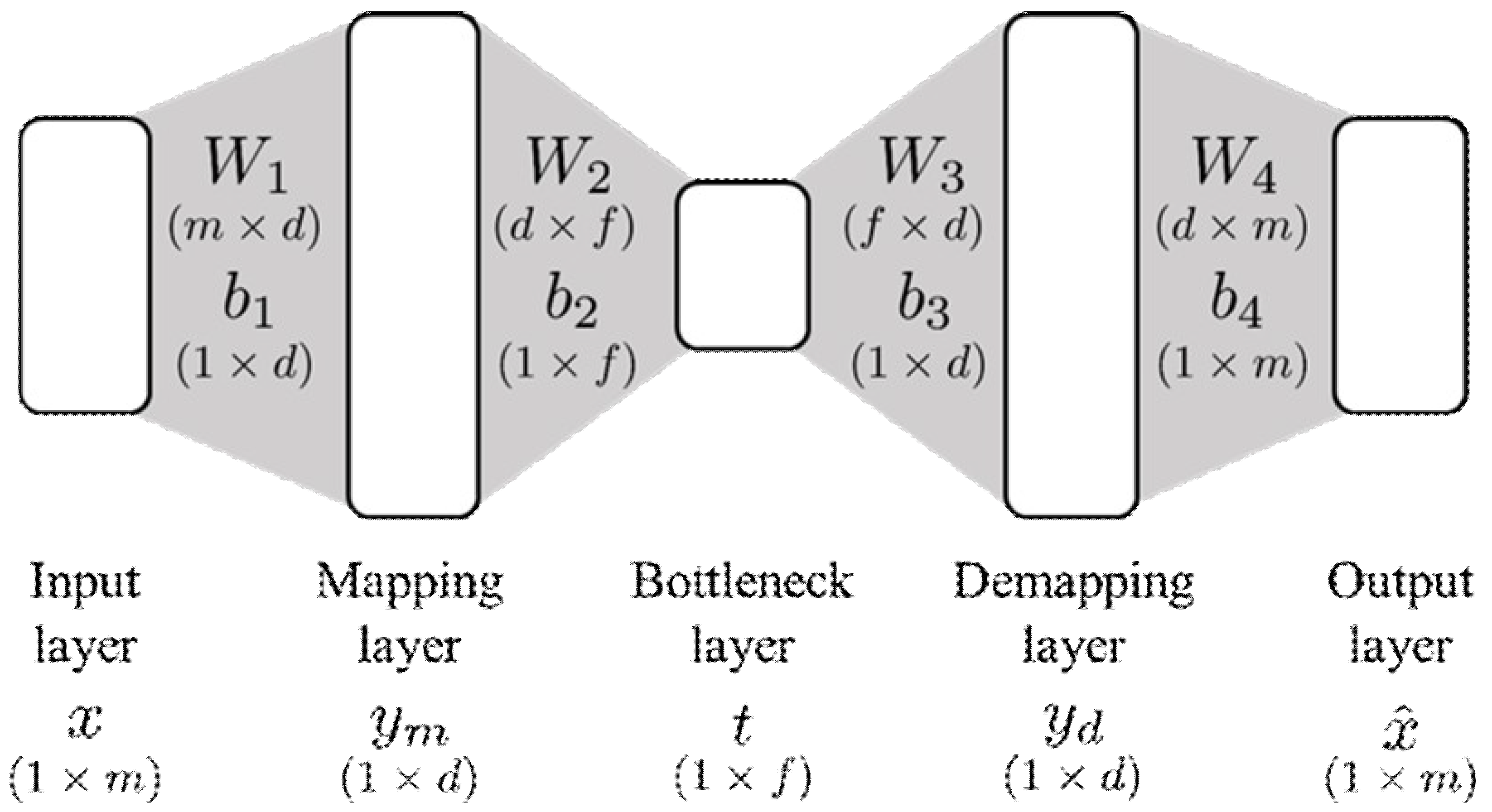
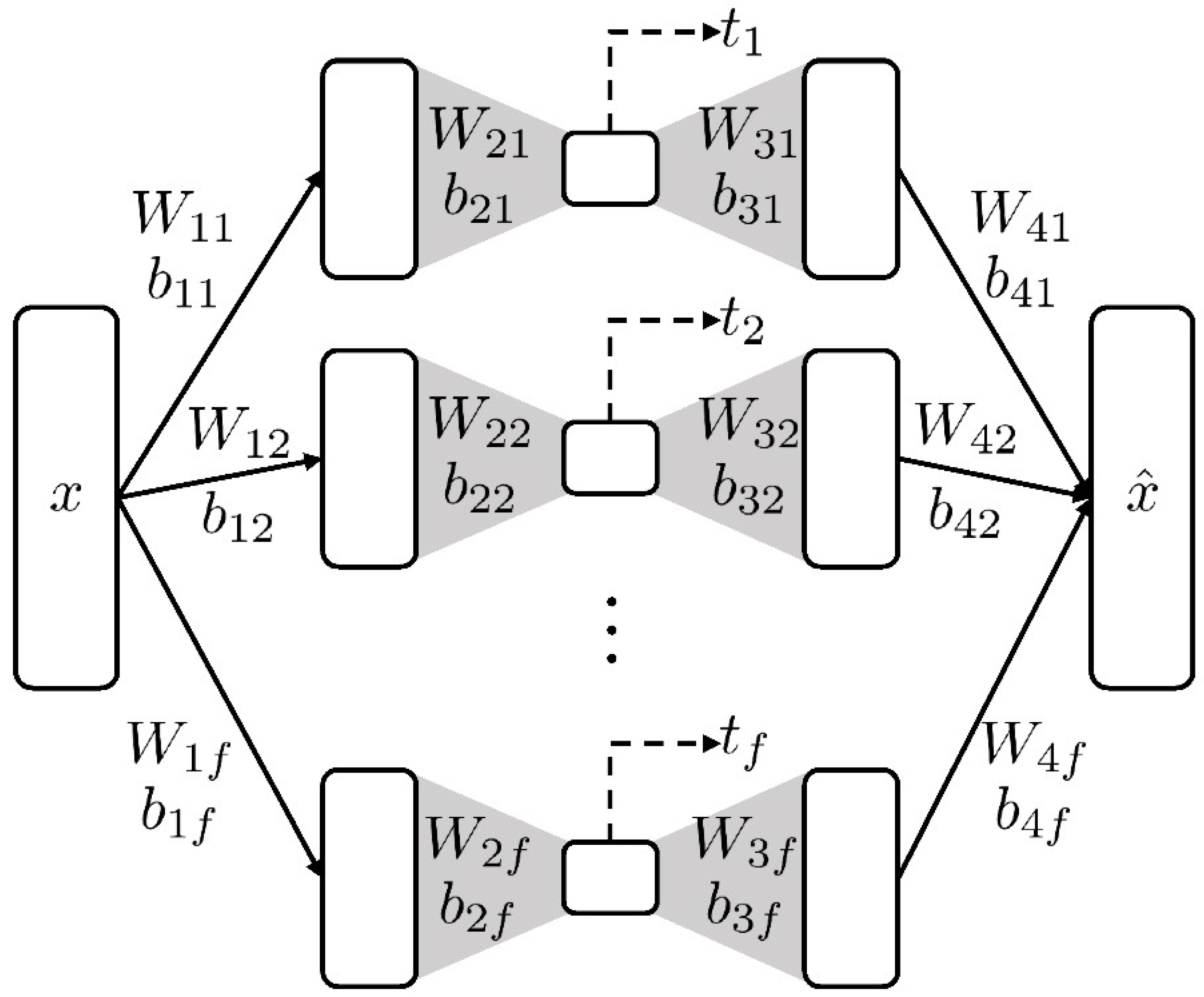
In this work, two neural network architectures were used to evaluate the NLPCA-based process monitoring. The NLPCA methods utilizing the networks shown in Figure 1 and Figure 2 will be referred to as sm-NLPCA (simultaneous NLPCA) and p-NLPCA (parallel NLPCA), respectively. The performance of the process monitoring was evaluated by two indices, fault detection rate (FDR) and false alarm rate (FAR). The effects of the following hyperparameters were analyzed:

• Number of hidden layers
• Number of mapping/demapping nodes
• Number of nonlinear principal components

We designed four different types of neural networks to evaluate the effects of the hyperparameters listed above. Types 1 and 2 had five layers (three hidden layers), while seven layers (five hidden layers) were used for Types 3 and 4. In Types 1 and 3, the numbers of mapping/demapping nodes were fixed at specific values, while they were proportional to the number of principal components to be extracted for Types 2 and 4. The number of parameters for different network types are summarized in

Table 3. Number of parameters for different neural network types.

	Neural Network Structure	Number of Parameters
		sm-NLPCA	p-NLPCA
Network type 1	52-100-f-100-52	210f + 10,652	f + 10,852
Network type 2	52-100f-f-100f-52	200f2 + 10,601f + 52	10,801f + 52
Network type 3	52-100-50-f-50-100-52	101f + 20,752	f + 10,852 + 10,000/f
Network type 4	52-100f-50f-f-50f-100f-52	10,100f2 + 10,701f + 52	20,801f + 52

. The numbers for the network structures represent the number of nodes in each layer starting from the input layer. Note that, for the same network type, p-NLPCA always had fewer parameters compared to sm-NLPCA due to the network decoupling.

Table 4. Process monitoring results with varying the neural network size (with five layers).

Network Type 1: 52-100-f-100-52
	sm-NLPCA				p-NLPCA
	T2		Q		T2		Q
f	FDR	FAR	FDR	FAR	FDR	FAR	FDR	FAR
5	0.4019	0.0085	0.7340	0.0144	0.4360	0.0091	0.7332	0.0136
10	0.5060	0.0089	0.7357	0.0146	0.5191	0.0094	0.7366	0.0141
15	0.4614	0.0097	0.7459	0.0156	0.5807	0.0094	0.7383	0.0146
20	0.4975	0.0093	0.7487	0.0174	0.5773	0.0094	0.7443	0.0160
Network Type 2: 52-100f-f-100f-52
	sm-NLPCA				p-NLPCA
	T2		Q		T2		Q
f	FDR	FAR	FDR	FAR	FDR	FAR	FDR	FAR
5	0.4754	0.0098	0.7440	0.0221	0.4501	0.0094	0.7445	0.0190
10	0.5861	0.0081	0.7889	0.0661	0.5433	0.0087	0.7507	0.0229
15	0.6232	0.0081	0.8427	0.1698	0.5850	0.0083	0.7603	0.0295
20	0.6254	0.0081	0.9038	0.3610	0.5953	0.0091	0.7737	0.0364

and

Table 5. Process monitoring results with varying the neural network size (with seven layers).

Network Type 3: 52-100-50-f-50-100-52
	sm-NLPCA				p-NLPCA
	T2		Q		T2		Q
f	FDR	FAR	FDR	FAR	FDR	FAR	FDR	FAR
5	0.4393	0.0086	0.7382	0.0141	0.3748	0.0088	0.7413	0.0143
10	0.4942	0.0085	0.7376	0.0142	0.4701	0.0090	0.7600	0.0140
15	0.5078	0.0088	0.7479	0.0157	0.4911	0.0099	0.7572	0.0134
20	0.5264	0.0088	0.7423	0.0146	0.5060	0.0093	0.7429	0.0122
Network Type 4: 52-100f-50f-f-50f-100f-52
	sm-NLPCA				p-NLPCA
	T2		Q		T2		Q
f	FDR	FAR	FDR	FAR	FDR	FAR	FDR	FAR
5	0.4439	0.0079	0.8018	0.0895	0.3769	0.0090	0.7500	0.0254
10	0.5821	0.0069	0.9796	0.8005	0.4683	0.0095	0.7744	0.0470
15	0.6057	0.0075	0.9997	0.9928	0.4916	0.0089	0.7841	0.0537
20	0.6032	0.0078	1.0000	0.9993	0.5283	0.0093	0.8138	0.0961

show the process monitoring results for Types 1 and 2 and Types 3 and 4, respectively. Note that, in this analysis, only the average value of FDR (over all the fault types) is reported for brevity.

The main trends to note are:

• The FDR in the residual space always showed a higher value than that in the principal component space, which matches the results reported in the literature where different techniques were utilized [45,46].
• In all network types, the FDR in the principal component space was improved with diminishing rates as the number of principal components increased.
• On the other hand, the number of principal components, which resulted in the best FDR value in the residual space, was different for different types of neural networks. As the size of the network became larger, the FAR in the residual space increased significantly, and sm-NLPCA completely failed when Network Type 4 was used, classifying the majority of the normal test data as faults. The main reason for this observation was the overfitting of the neural networks. Despite the network overfitting, the FDR in the principal component space was increased by adding more nodes in the mapping/demapping layers, while the FAR in the principal component space was not affected by such addition.

Regarding the last point, in the case of the demapping functions, the input had a lower dimension than the output, which made the problem of approximating demapping functions ill-posed. Thus, it can be speculated that the network overfitting mainly occurred during the reconstruction of the data (i.e., demapping functions were overfitted), leaving the results in the principal component space unaffected by the network overfitting. In addition to this, it was observed that, by including more nodes in the mapping/demapping layers, the average standard deviation of the principal components was increased by a factor of 2~8. This implies that, in Network Types 2 and 4, the normal operating region in the principal component space was more “loosely” defined (i.e., the normal data cluster had a larger volume) compared to Network Types 1 and 3, which can make the problem of approximating the demapping functions more ill-posed. It can also be a reason why the FAR in the principal component space was consistently low regardless of the network size and the degree of network overfitting.

Table 6. Fault detection rates with adjusted upper control limits (FAR = 0.01 for normal test data).

	Network Type 1				Network Type 2
	sm-NLPCA		p-NLPCA		sm-NLPCA		p-NLPCA
f	T2	Q	T2	Q	T2	Q	T2	Q
5	0.4082	0.7246	0.4406	0.7256	0.4767	0.7214	0.4526	0.7268
10	0.5098	0.7265	0.5208	0.7285	0.5917	0.7262	0.5472	0.7293
15	0.4629	0.7341	0.5823	0.7289	0.6284	0.7257	0.5891	0.7303
20	0.4992	0.7316	0.5791	0.7313	0.6305	0.7253	0.5975	0.7331
	Network Type 3				Network Type 4
	sm-NLPCA		p-NLPCA		sm-NLPCA		p-NLPCA
f	T2	Q	T2	Q	T2	Q	T2	Q
5	0.4441	0.7297	0.3787	0.7314	0.4523	0.7225	0.3804	0.7234
10	0.4997	0.7294	0.4737	0.7507	0.5920	0.6951	0.4706	0.7245
15	0.5116	0.7350	0.4916	0.7490	0.6128	0.6887	0.4967	0.7261
20	0.5297	0.7327	0.5079	0.7377	0.6096	0.6866	0.5307	0.7251

shows the FDR values obtained by adjusting the upper control limits such that the FAR became 0.01 for the normal test data. The following can be clearly seen:

• sm-NLPCA performed better than p-NLPCA in the principal component space, while p-NLPCA was better in the residual space.

By comparing the results from Network Types 1 and 3, adding additional hidden layers was shown to improve the FDR in the principal component space for sm-NLPCA and the FDR in the residual space for p-NLPCA. However, the effects of such addition cannot be evaluated clearly for Network Types 2 and 4. Thus, in what follows, we apply the neural network regularization techniques to Network Types 2 and 4 and evaluate the effects of such techniques on the performance of NLPCA-based process monitoring.

4.3. Neural Network Regularization

In this analysis, we consider three different types of neural network regularization: dropout and L₁ and L₂ regularizations. Dropout is a neural network regularization technique, where randomly-selected nodes and their connections are dropped during the network training to prevent co-adaptation [47]. L₁ and L₂ regularizations prevent network overfitting by putting constraints on the L₁ norm and L₂ norm of the weight matrices, respectively.

The process monitoring results for Network Types 2 and 4 are tabulated in

Table 7. Process monitoring results with neural network regularization (Network Type 2).

sm-NLPCA
	No Regularization				L1 Regularization				L2 Regularization
	T2		Q		T2		Q		T2		Q
f	FDR	FAR	FDR	FAR	FDR	FAR	FDR	FAR	FDR	FAR	FDR	FAR
10	0.5861	0.0081	0.7889	0.0661	0.4870	0.0096	0.7358	0.0155	0.5151	0.0093	0.7358	0.0249
15	0.6232	0.0081	0.8427	0.1698	0.4867	0.0099	0.7411	0.0274	0.5288	0.0095	0.7403	0.0175
20	0.6254	0.0081	0.9038	0.3610	0.5352	0.0100	0.7448	0.0208	0.5867	0.0088	0.7443	0.0204
p-NLPCA
	No Regularization				L1 Regularization				L2 Regularization
	T2		Q		T2		Q		T2		Q
f	FDR	FAR	FDR	FAR	FDR	FAR	FDR	FAR	FDR	FAR	FDR	FAR
10	0.5433	0.0087	0.7507	0.0229	0.5201	0.0087	0.7532	0.0234	0.5065	0.0087	0.7503	0.0237
15	0.5850	0.0083	0.7603	0.0295	0.5711	0.0087	0.7649	0.0321	0.5532	0.0086	0.7647	0.0333
20	0.5995	0.0091	0.7737	0.0364	0.5905	0.0090	0.7769	0.0401	0.5868	0.0090	0.7796	0.0420

and

Table 8. Process monitoring results with neural network regularization (Network Type 4).

sm-NLPCA
	No Regularization				L1 Regularization				L2 Regularization				Dropout
	T2		Q		T2		Q		T2		Q		T2		Q
f	FDR	FAR	FDR	FAR	FDR	FAR	FDR	FAR	FDR	FAR	FDR	FAR	FDR	FAR	FDR	FAR
10	0.5821	0.0069	0.9796	0.8005	0.4086	0.0088	0.7360	0.0142	0.4881	0.0089	0.7535	0.0292	0.5091	0.0082	0.7435	0.0141
15	0.6057	0.0075	0.9997	0.9928	0.5507	0.0098	0.7375	0.0143	0.5697	0.0087	0.7685	0.0412	0.4866	0.0081	0.7600	0.0197
20	0.6032	0.0078	1.0000	0.9993	0.5870	0.0087	0.7331	0.0128	0.6159	0.0087	0.7975	0.0817	0.5346	0.0083	0.7852	0.0405
p-NLPCA
	No Regularization				L1 Regularization				L2 regularization				Dropout
	T2		Q		T2		Q		T2		Q		T2		Q
f	FDR	FAR	FDR	FAR	FDR	FAR	FDR	FAR	FDR	FAR	FDR	FAR	FDR	FAR	FDR	FAR
10	0.4683	0.0095	0.7744	0.0470	0.4469	0.0090	0.7695	0.0363	0.4721	0.0085	0.7715	0.0452	0.4988	0.0091	0.7577	0.0208
15	0.4916	0.0089	0.7841	0.0537	0.4671	0.0092	0.7774	0.0412	0.4940	0.0094	0.7903	0.0638	0.5120	0.0095	0.7602	0.0191
20	0.5283	0.0093	0.8138	0.0961	0.5114	0.0096	0.7774	0.0347	0.5433	0.0086	0.8034	0.0766	0.5481	0.0094	0.7714	0.0216

, respectively. In the case of Network Type 2, dropout did not address the problem of overfitting for p-NLPCA, and therefore, the results obtained using dropout are not presented here.

• In most cases, neural network regularization degraded the process monitoring performance in the principal component space with p-NLPCA of Network Type 4 regularized by dropout being the only exception.
• On the other hand, it dramatically reduced the FAR values in the residual space for sm-NLPCA, while such reduction was not significant for p-NLPCA (the FAR in the residual space even increased for Network Type 2). This indicates that overfitting was a problem for the residual space detection using sm-NLPCA.

Table 9. Process monitoring results with network regularization and adjusted upper control limits (FAR = 0.01 for the normal test data).

Network Type 2
	sm-NLPCA								p-NLPCA
	No Regularization		L1		L2		Dropout		No Regularization		L1		L2		Dropout
f	T2	Q	T2	Q	T2	Q	T2	Q	T2	Q	T2	Q	T2	Q	T2	Q
10	0.5917	0.7262	0.4884	0.7254	0.5173	0.7248	-	-	0.5472	0.7293	0.5239	0.7309	0.5113	0.7280	-	-
15	0.6284	0.7257	0.4872	0.7266	0.5304	0.7268	-	-	0.5891	0.7303	0.5746	0.7316	0.5577	0.7300	-	-
20	0.6305	0.7253	0.5357	0.7236	0.5904	0.7248	-	-	0.5975	0.7331	0.5932	0.7319	0.5897	0.7321	-	-
Network Type 4
	sm-NLPCA								p-NLPCA
	No Regularization		L1		L2		Dropout		No Regularization		L1		L2		Dropout
f	T2	Q	T2	Q	T2	Q	T2	Q	T2	Q	T2	Q	T2	Q	T2	Q
10	0.5920	0.6951	0.4145	0.7279	0.4922	0.7249	0.5148	0.7357	0.4706	0.7245	0.4517	0.7285	0.4780	0.7235	0.5015	0.7372
15	0.6128	0.6887	0.5519	0.7294	0.5737	0.7244	0.4928	0.7419	0.4967	0.7261	0.4705	0.7309	0.4936	0.7245	0.5134	0.7422
20	0.6096	0.6866	0.5908	0.7277	0.6194	0.7225	0.5404	0.7492	0.5307	0.7251	0.5133	0.7338	0.5476	0.7256	0.5499	0.7483

shows the process monitoring results obtained by adjusting the upper control limits as mentioned in the previous analysis. Overall, p-NLPCA performed better than sm-NLPCA, while sm-NLPCA was better than p-NLPCA in the principal component space when Network Type 4 was used. By comparing the results provided in Table 6 and Table 9, it can be seen that having more nodes in the mapping/demapping layers is only beneficial to the process monitoring in the principal component space. Putting more nodes implies the increased complexity of the functions approximated by neural networks. Thus, it makes the problem of approximating demapping functions more ill-posed and has the potential to be detrimental to the performance of process monitoring in the residual space. Although neural network regularization techniques can reduce the stiffness and complexity of the functions approximated by neural networks [48], they seem to be unable to define better boundaries for one-class classifiers.

4.4. Network Training Objective Function

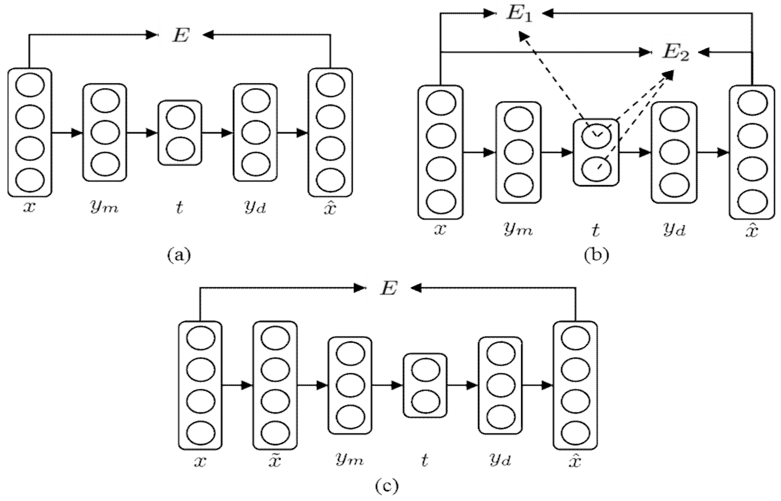
Let us now evaluate the effects of different objective functions on the process monitoring performance. For illustration purposes, only Network Type 4 was considered in this analysis. All the values of α_k were set to one for the hierarchical error, and the corrupted input was generated by using a Gaussian noise of zero mean and 0.1 standard deviation for the denoising criterion. L₂ regularization and L₁ regularization were used to prevent overfitting for sm-NLPCA and p-NLPCA, respectively.

Table 10. Process monitoring results with different neural network training objective functions.

sm-NLPCA
	Reconstruction Error				Hierarchical Error				Denoising
	T2		Q		T2		Q		T2		Q
f	FDR	FAR	FDR	FAR	FDR	FAR	FDR	FAR	FDR	FAR	FDR	FAR
10	0.4881	0.0089	0.7535	0.0292	0.5869	0.0099	0.7312	0.0137	0.4203	0.0096	0.7347	0.0147
15	0.5697	0.0087	0.7685	0.0412	0.5940	0.0084	0.7367	0.0161	0.5253	0.0090	0.7393	0.0150
20	0.6159	0.0087	0.7975	0.0817	0.5918	0.0082	0.7628	0.0398	0.5821	0.0084	0.7483	0.0181
p-NLPCA
	Reconstruction Error				Hierarchical Error				Denoising
	T2		Q		T2		Q		T2		Q
f	FDR	FAR	FDR	FAR	FDR	FAR	FDR	FAR	FDR	FAR	FDR	FAR
10	0.4469	0.0090	0.7695	0.0363	0.3854	0.0092	0.7705	0.0428	0.4260	0.0093	0.7374	0.0121
15	0.4671	0.0092	0.7774	0.0412	0.4736	0.0085	0.7877	0.0572	0.4749	0.0095	0.7445	0.0123
20	0.5114	0.0096	0.7774	0.0347	0.5397	0.0089	0.7975	0.0658	0.5122	0.0093	0.7469	0.0121

and

Table 11. Process monitoring results with different neural network training objective functions and adjusted upper control limits (FAR = 0.01 for normal test data).

sm-NLPCA
	Reconstruction Error		Hierarchical Error		Denoising
f	T2	Q	T2	Q	T2	Q
10	0.4922	0.7249	0.5874	0.7241	0.4223	0.7258
15	0.5737	0.7244	0.5985	0.7259	0.5292	0.7295
20	0.6194	0.7225	0.5975	0.7281	0.5879	0.7315
p-NLPCA
	Reconstruction Error		Hierarchical Error		Denoising
f	T2	Q	T2	Q	T2	Q
10	0.4517	0.7285	0.3890	0.7235	0.4291	0.7323
15	0.4705	0.7309	0.4797	0.7258	0.4766	0.7393
20	0.5133	0.7338	0.5429	0.7245	0.5146	0.7412

summarize the process monitoring results obtained by using the autoassociative neural networks trained with different objective functions.

The following are the major trends to note:

• The monitoring performance of sm-NLPCA in the principal component space became more robust by using the hierarchical error, showing similar FDR values regardless of the number of principal components.
• However, the FDR value in the principal component space scaled better with the reconstruction error objective function. On the other hand, the monitoring performance of p-NLPCA in the principal component space became more sensitive to the number of principal components with the hierarchical error as the objective function. As a result, the FDR value in the principal component space was improved when the number of principal components was 20.
• While the hierarchical error provided a slight improvement to the monitoring performance in the residual space for sm-NLPCA, it degraded the performance of p-NLPCA in the residual space.
• The denoising criterion was beneficial to both NLPCA methods in the residual space, improving the FDR values when the upper control limits were adjusted. The monitoring performance of p-NLPCA in the principal component space was not affected by using the denoising criterion, while that of sm-NLPCA deteriorated.

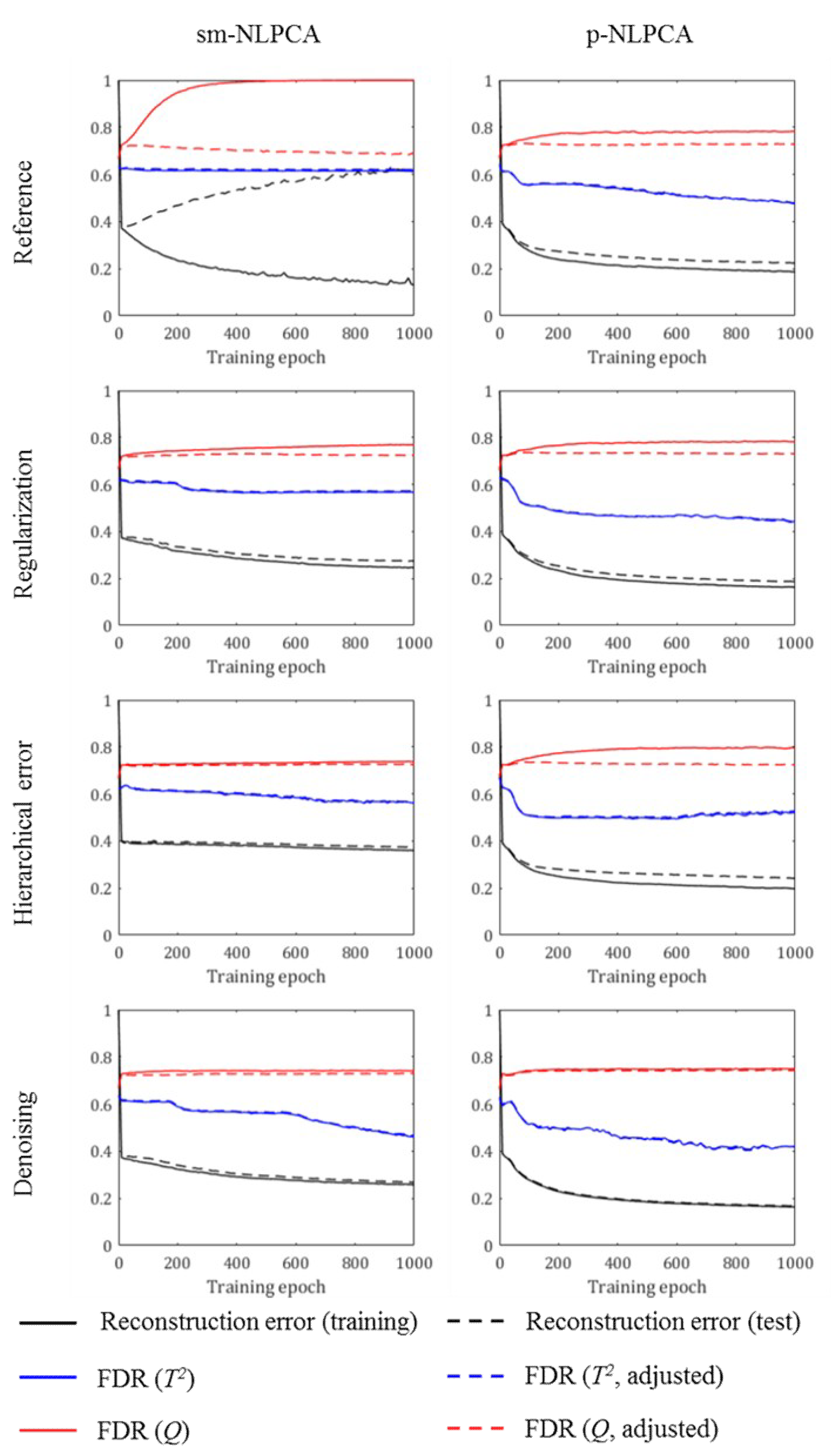
4.5. Neural Network Training Epochs

In this analysis, the effects of neural network training epochs are analyzed. To this end, Network Type 4 with 15 principal components was trained, and the neural network parameters were saved at every 10 epochs. Figure 4 shows how different values evolve as the neural networks are trained. For the reference case, the neural networks were trained without any regularization and with the reconstruction error as the objective function. It can be clearly seen that the network overfitting (which is captured by the difference between the solid and dashed black lines) resulted in high FAR values in the residual space (which is captured by the difference between the solid and dashed red lines), while it did not affect the FAR values in the principal component space (which is captured by the difference between the solid and dashed blue lines).

Note the following:

• Despite the decrease in the reconstruction error over a wide range of training epochs, the adjusted FDR value in the residual space increased during only the first few training epochs and was kept almost constant in the rest of the training.
• In some cases, there was even a tendency that the adjusted FDR value in the principal component space decreased as the network was trained more.

Thus, during the network training, it was required to monitor both reconstruction error and process monitoring performance indices, and early stopping needed to be applied as necessary to ensure high monitoring performances. Nonetheless, from the above observations, it can be concluded that the objective functions available in the literature, which focus on the reconstruction ability of the autoassociative neural networks, may not be most suitable for the design of one-class classifiers. This necessitates the development of alternative training algorithms of autoassociative neural networks to improve the performance of neural-network-based one-class classifiers.

4.6. Comparison with Linear-PCA-Based Process Monitoring

Let us finally compare the NLPCA-based process monitoring with the linear-PCA-based one. For the linear-PCA-based process monitoring, based on the parallel analysis [35], the number of principal components to be retained was selected as 15. The same number of principal components was used in the NLPCA-based process monitoring. For sm-NLPCA, the following setting was used: Network Type 2, no regularization, reconstruction error as the objective function. For p-NLPCA, the following setting was used: Network Type 3, no regularization, reconstruction error as the objective function.

Table 12. Detailed process monitoring results obtained using linear PCA and two NLPCA methods (FAR = 0.01 for normal test data).

Fault ID	Linear PCA		sm-NLPCA		p-NLPCA
	T2	Q	T2	Q	T2	Q
1	0.9926	0.9965	0.9931	0.9963	0.9891	0.9967
2	0.9848	0.9864	0.9849	0.9863	0.9841	0.9870
4	0.0916	0.9939	0.1375	0.9830	0.0939	0.9983
5	0.2404	0.1192	0.2461	0.2028	0.3312	0.7922
6	0.9896	1.0000	0.9939	1.0000	0.9968	1.0000
7	1.0000	0.9998	0.9994	1.0000	0.9990	1.0000
8	0.9637	0.9541	0.9634	0.9651	0.8827	0.9656
10	0.1960	0.1586	0.2436	0.1896	0.0860	0.2195
11	0.2953	0.6901	0.2995	0.6670	0.1415	0.7141
12	0.9785	0.9563	0.9773	0.9769	0.9008	0.9810
13	0.9353	0.9425	0.9378	0.9436	0.8974	0.9452
14	0.9549	0.9995	0.9457	0.9995	0.7661	0.9996
16	0.0706	0.0974	0.0944	0.1131	0.0361	0.1547
17	0.7177	0.8816	0.7173	0.8779	0.6200	0.8922
18	0.9270	0.9337	0.9270	0.9345	0.9131	0.9358
19	0.0819	0.0845	0.0431	0.1114	0.0222	0.1003
20	0.2535	0.4395	0.2775	0.4420	0.1271	0.4737
Average	0.6278	0.7196	0.6342	0.7288	0.5757	0.7739

tabulates the process monitoring results obtained using three different PCA methods. Note that the upper control limits were adjusted to have FAR values of 0.01. The main trends observed were:

• Compared to the linear PCA, the process monitoring results in both spaces were improved slightly by using sm-NLPCA. The most significant improvements were obtained for Faults 4 and 10 in the principal component space and Faults 5 and 10 in the residual space.
• On the other hand, p-NLPCA showed a lower performance than linear PCA in the principal component space, while the performance in the residual space was significantly improved. The adjusted FDR value in the residual space from p-NLPCA was higher than that from the linear PCA for all the fault types, with Faults 5, 10, and 16 being the most significant ones.

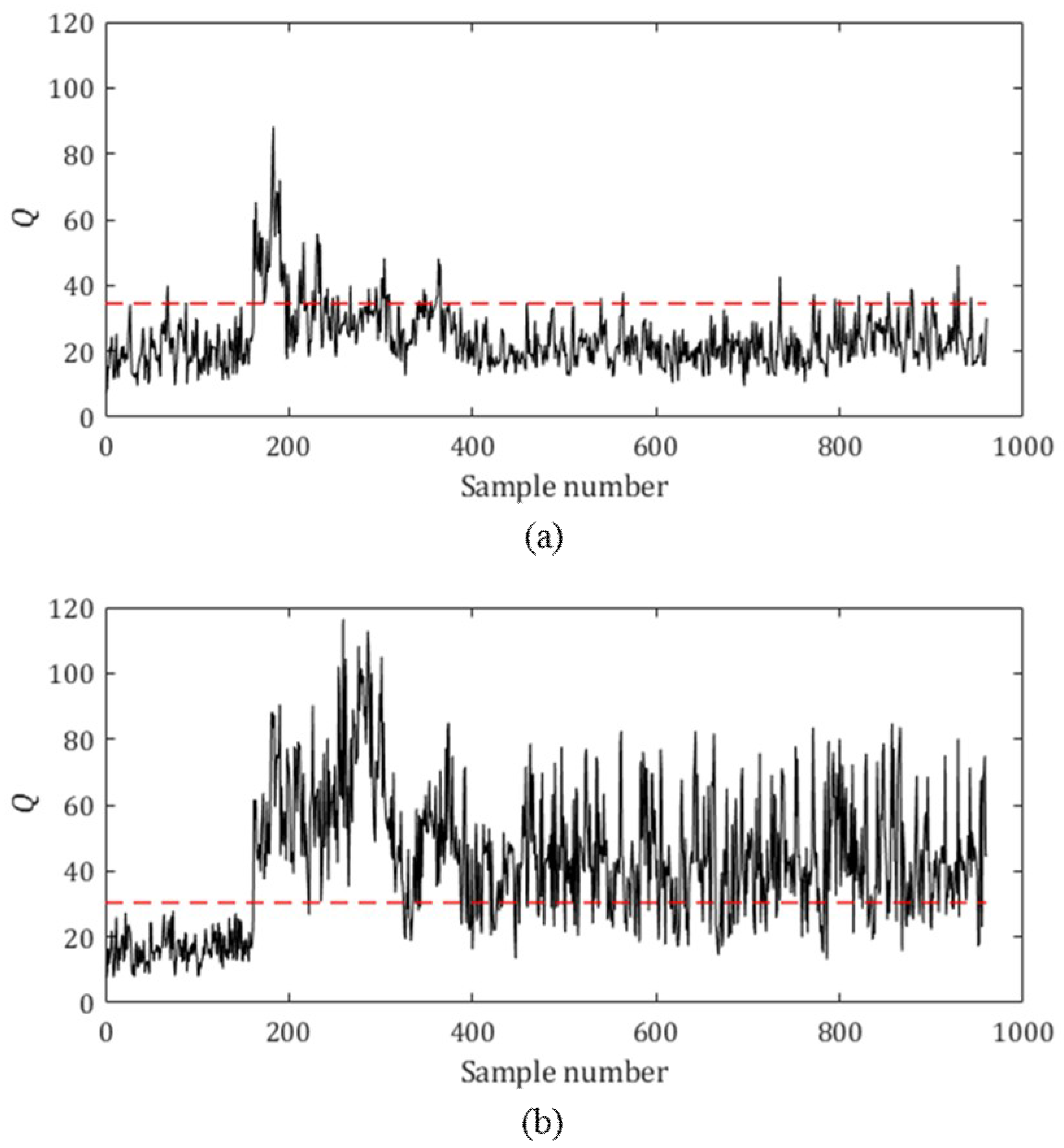
Let us consider two cases that illustrate the advantages of p-NLPCA over the linear PCA as the basis for the process monitoring system design. Figure 5 shows the Q statistic values (black solid line) for one complete simulation run with Fault 5, along with the upper control limit (dashed red line). Although both linear PCA and p-NLPCA detected the fault very quickly (fault introduced after Sample Number 160 and detected at Sample Number 162), in the case of the linear PCA, the Q statistic value dropped below the upper control limit after around Sample Number 400. The Q statistic value calculated from p-NLPCA did not decrease much, indicating that the fault was not yet removed from the system.

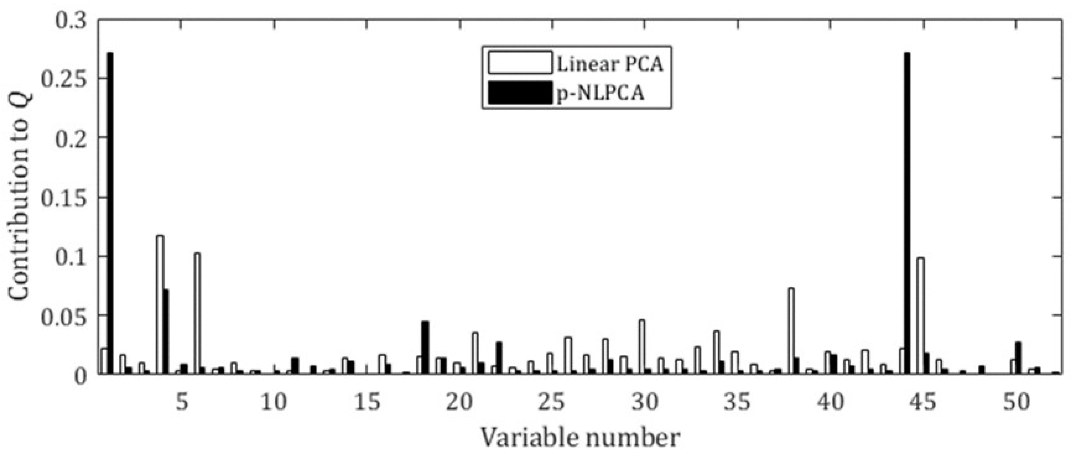
The contribution plots of Q statistic for Fault 1, which involves a step change in the flowrate of the A feed stream, are provided in Figure 6. In the case of the linear PCA, the variables with the highest contribution to the Q statistic were Variables 4 and 6, which are the flowrates of Stream 4 (which contains both A and C) and the reactor feed rate, respectively. Note that although these variables were also highly affected by the fault, they were not the root cause of the fault. On the other hand, in the case of p-NLPCA, the variables with the highest contribution to the Q statistic were Variables 1 and 44, which both represent the flowrate of the A feed stream, the root cause of the fault. Thus, it can be concluded that the process monitoring using p-NLPCA showed some potential to perform better at identifying the root cause of the fault introduced to the system.

5. Conclusions

The statistical process monitoring problem of the Tennessee Eastman process was considered in this study using autoassociative neural networks to define normal operating regions. Using the large dataset allowed us to estimate the upper control limits for the process monitoring directly from the data distribution and to train relatively large neural networks without overfitting. It was shown that the process monitoring performance was very sensitive to the neural network settings such as neural network size and neural network regularization. p-NLPCA was shown to be more effective for the process monitoring than the linear PCA and sm-NLPCA in the residual space, while its performance was worse than the others in the principal component space. p-NLPCA also showed the potential of better fault diagnosis capability than the linear PCA, locating the root cause more correctly for some fault types.

There still exist several issues that need to be addressed to make autoassociative neural networks more attractive as a tool for statistical process monitoring. First, a systematic procedure needs to be developed to provide a guideline for the design of optimal autoassociative neural networks to be used for the statistical process monitoring. Furthermore, a new neural network training algorithm may be required to extract principal components that are more relevant to the process monitoring tasks. Finally, the compatibility of different techniques to define the upper control limits, other than the T² and Q statistics, needs to be extensively evaluated.