A Risk Aversion Dispatching Optimal Model for a Micro Energy Grid Integrating Intermittent Renewable Energy and Considering Carbon Emissions and Demand Response

 ,
,
Abstract
1. Introduction
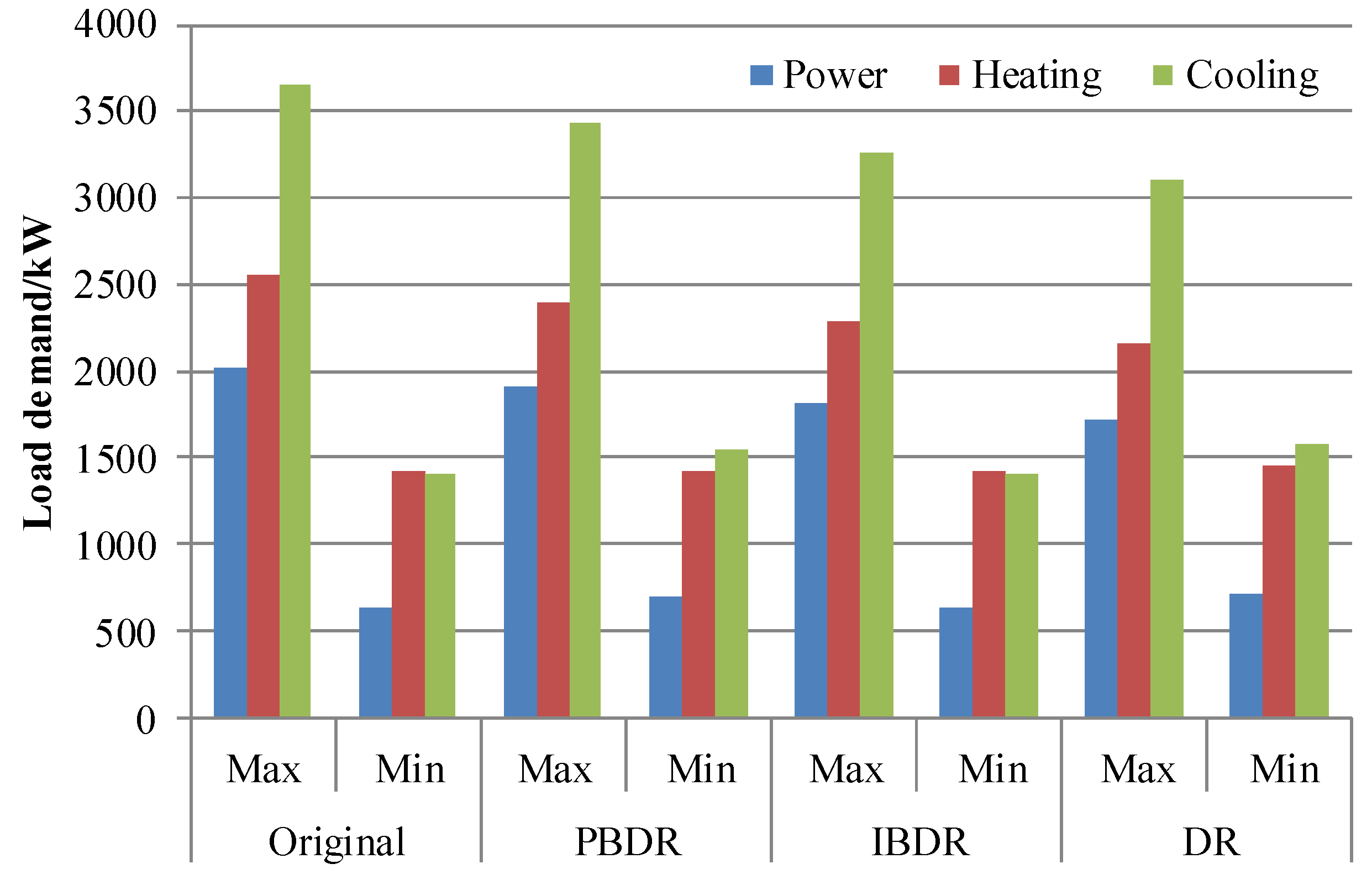
- This paper designs a novel structure for a micro energy grid optimal operation containing production devices, conversion devices, and storage devices, depending on the demand response and carbon emissions. The effects of price-based demand response (PBDR) and incentive-based demand response (IBDR) on different energy load curves are compared and analyzed. The optimization effect of the maximum total emission allowance (MTEA) on the MEG operation is also analyzed.
- This paper establishes a basic dispatching model for the micro energy grid considering different constraints, selecting maximizing operating revenue as the objective function of the MEG operation with the constraints of load power balance, equipment operation, DR operation, maximum carbon emissions, and rotating standby.
- This paper puts forward a risk aversion model for the micro energy grid on the basis of the CVaR method and robust stochastic optimization theory. The CVaR method mainly describes the influence of uncertainty factors of the objective function, and robust stochastic optimization theory converts constraints with uncertainty variables to provide an optimal basis for decision makers.
2. MEG Description and Output Model
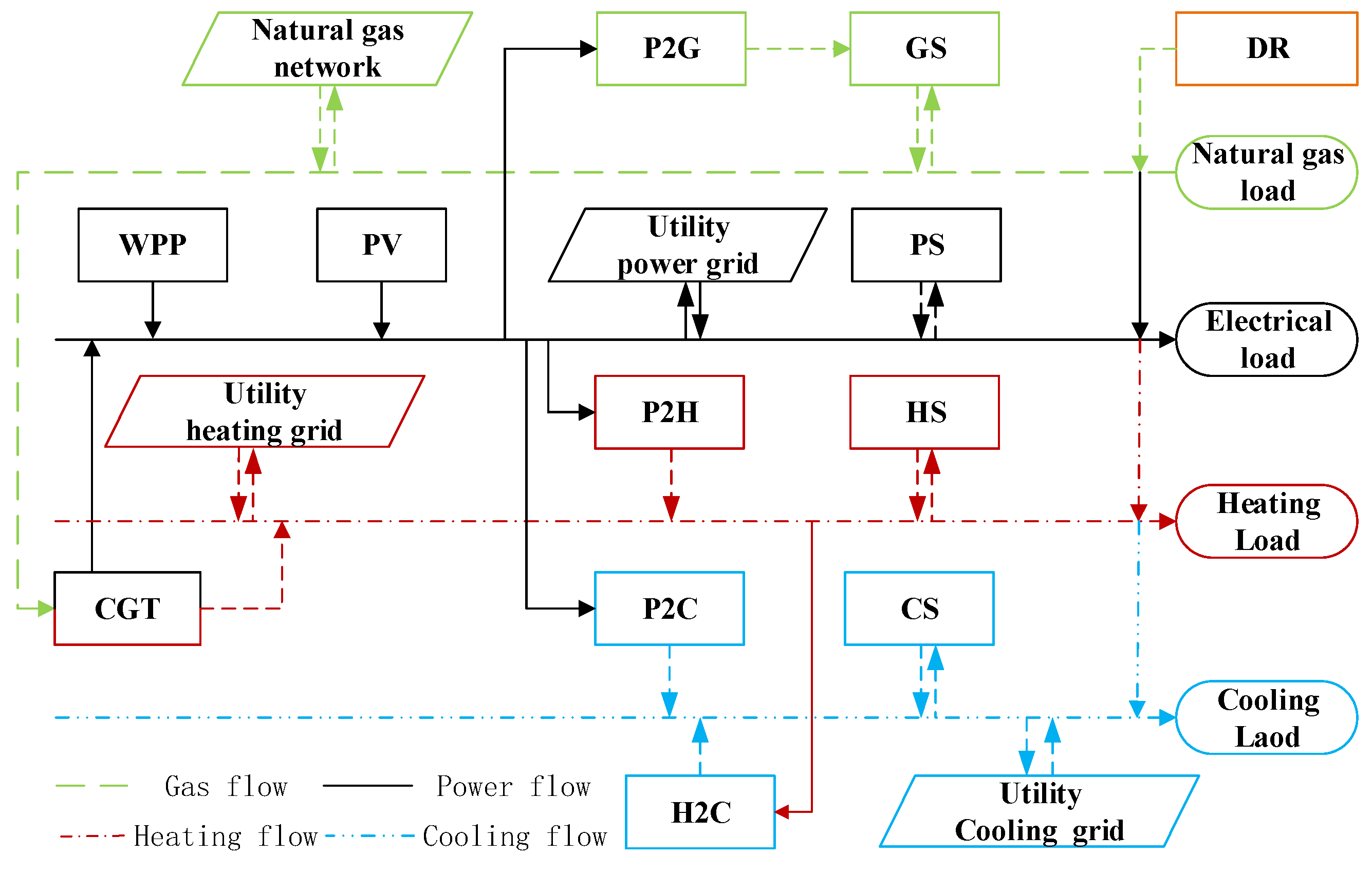
2.1. Structure Description
2.2. Energy Devices Operation Model
2.2.1. EP Operation Model
2.2.2. EC Operation Model
2.2.3. ES Operation Model
2.3. DR Operation Model
2.3.1. PBDR Operation Model
2.3.2. IBDR Operation Model
3. Basic Dispatching Model of the Micro Energy Grid
3.1. Objective Functions
3.2. Condition Constraints
4. Risk Aversion Model of the Micro Energy Grid
4.1. Uncertainty Factors Analysis
4.2. Risk Aversion Optimal Model
5. Example Analyses
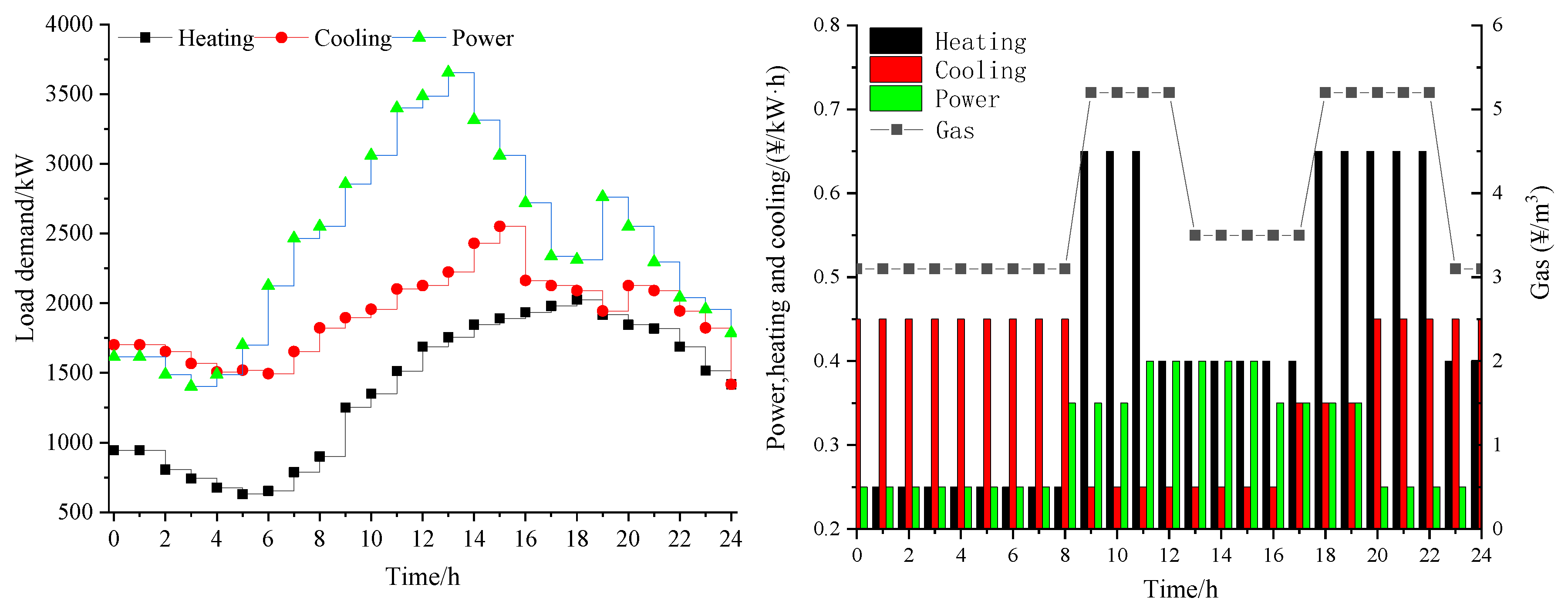
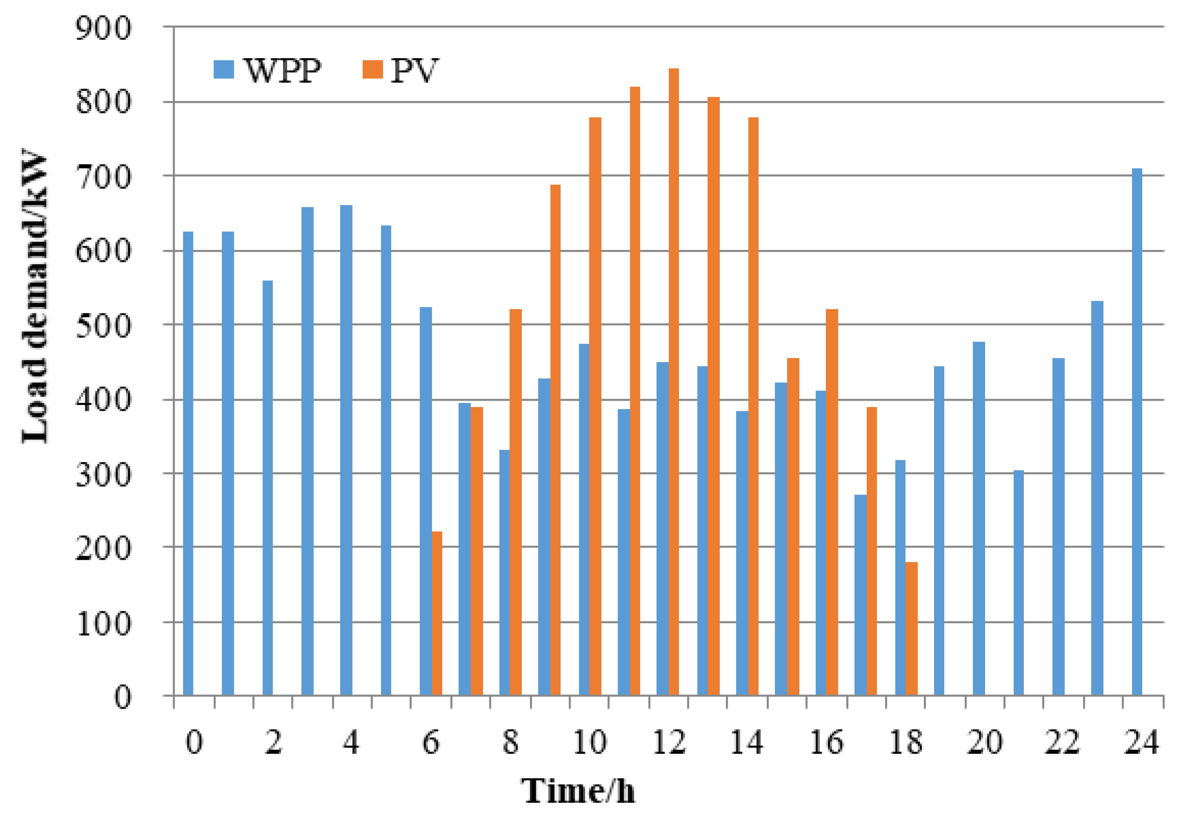
5.1. Basic Data
- Case 1: Basic scenario, scheduling of the MEG without uncertainty. This scenario does not take the uncertainty of WPP and PV into account. It analyzes the operation character of different compositions of the MEG and focuses on the complementary effects among them.
- Case 2: scenario with CVaR, dispatching of the MEG with the CVaR method. The scenario focuses on WPP and PV output uncertainty. CVaR is applied to change the objective function. By comparing and analyzing the scheduling result of MEG operation under different values of confidence β, the effectiveness of CVaR in dealing with the uncertainty of WPP and PV is verified.
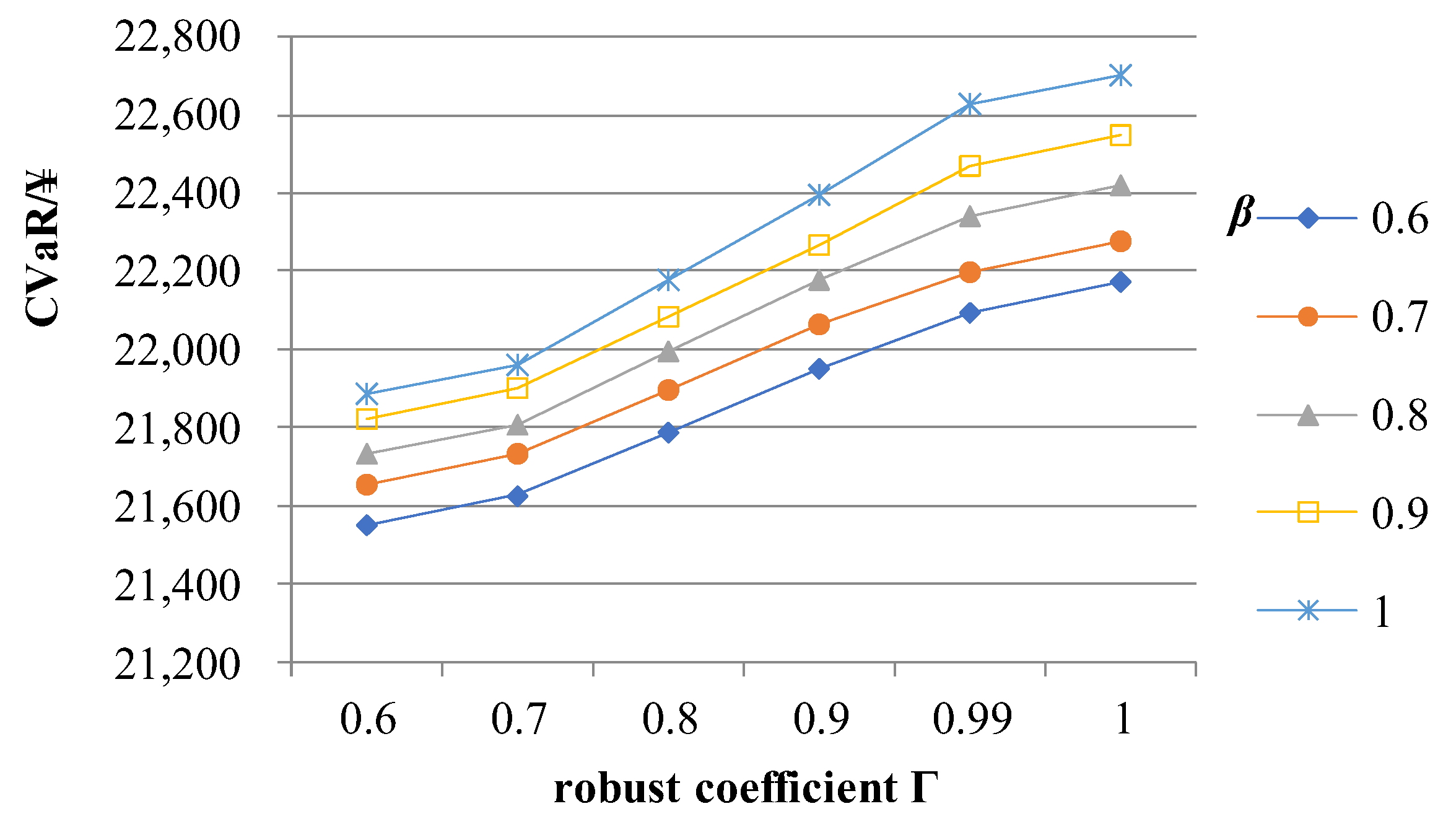
- Case 3: Comprehensive scenario, dispatching of MEG with the CVaR-robust method. The scenario constructs stochastic constraints using robust stochastic optimization theory, and discusses the MEG dispatching optimal strategy with different robustness and prediction accuracy values, and analyzes the validity of the CVaR-robust method.
5.2. Example Results
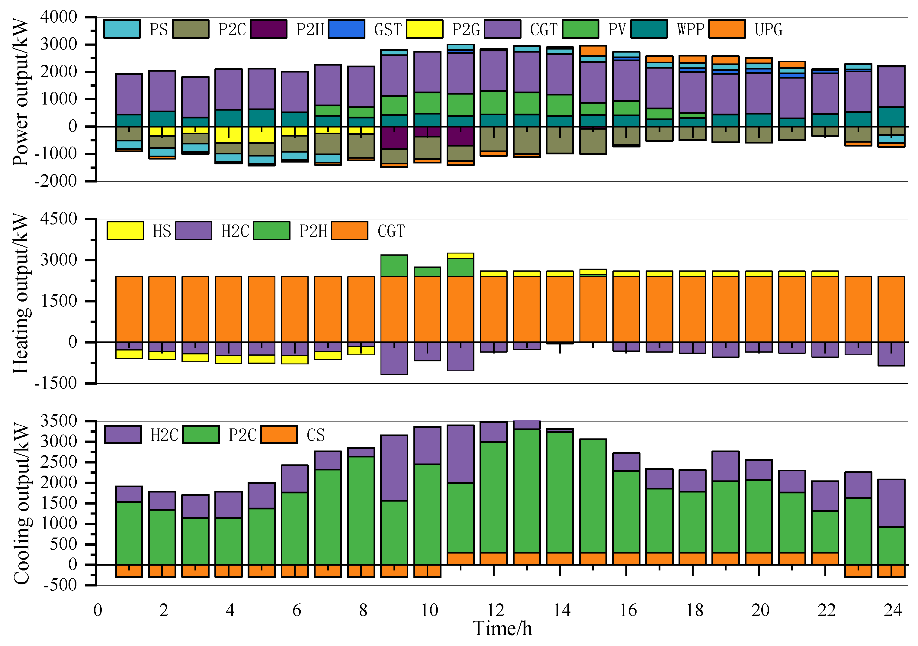
5.2.1. Scheduling Results of Case 1
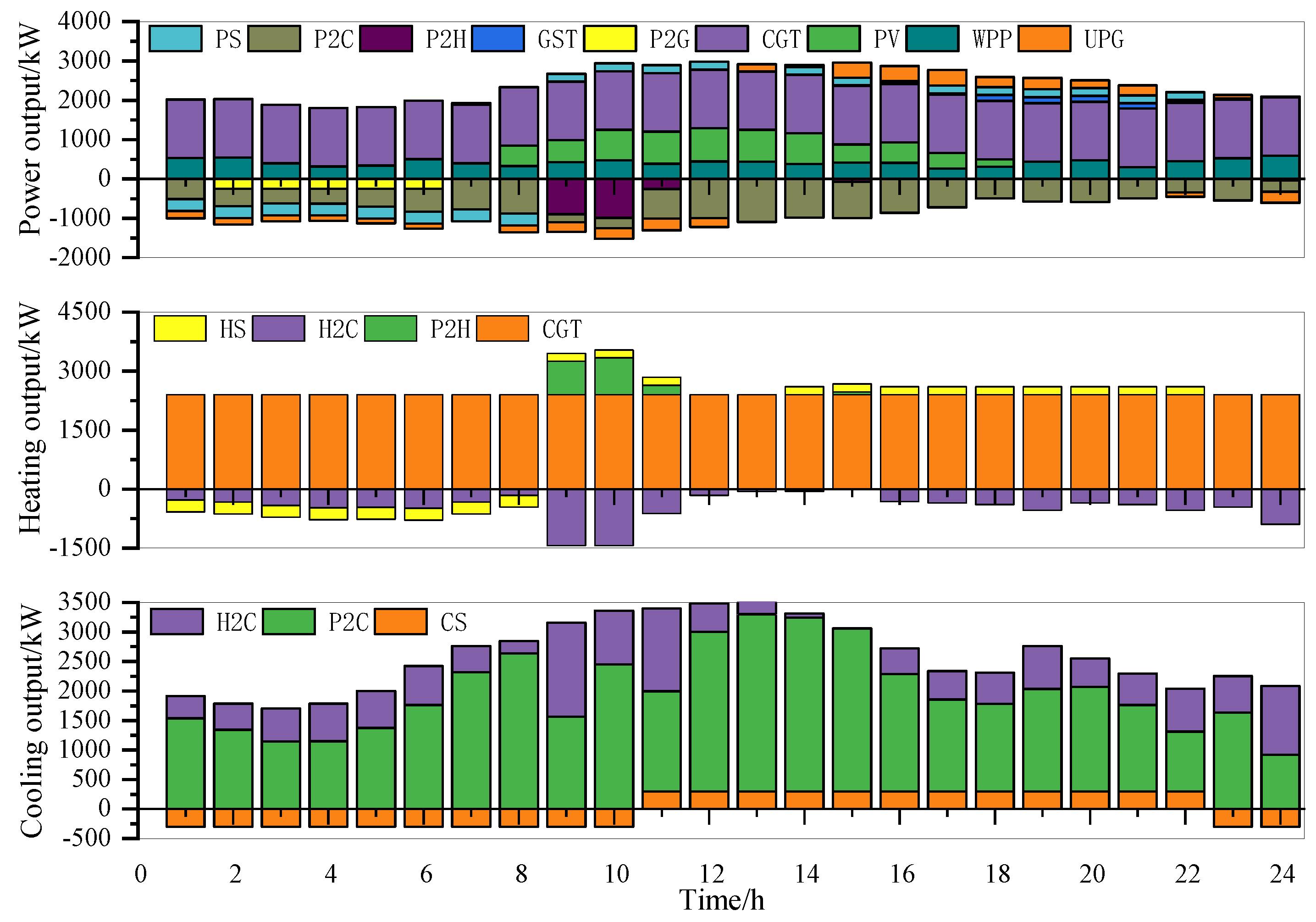
5.2.2. Scheduling Results of Case 2
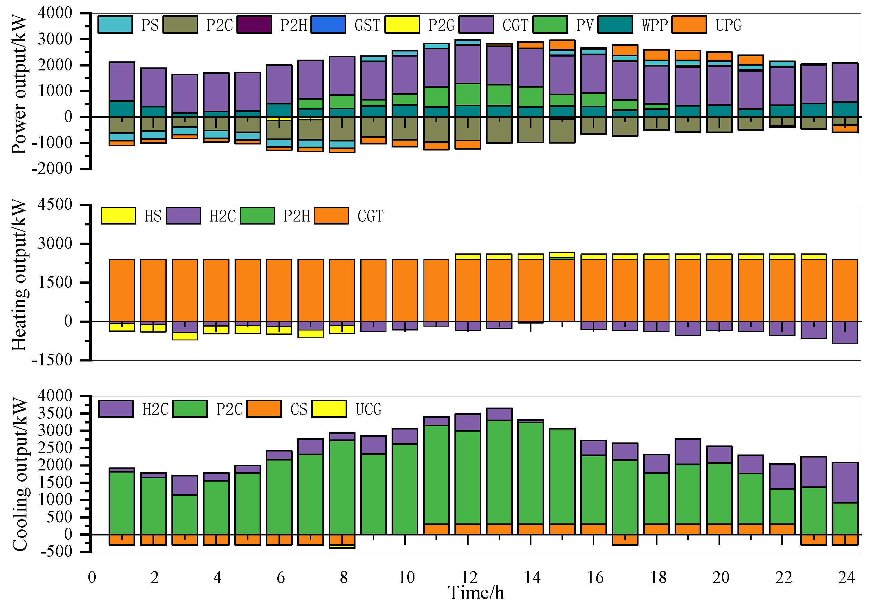
5.2.3. Scheduling Results of Case 3
5.3. Results Analysis
6. Conclusions
Author Contributions
Funding
Conflicts of Interest
Nomenclature
| Abbreviation | |
| MEG | micro energy grid |
| MTEA | maximum total carbon emission allowance |
| WPP | wind power plant |
| PV | photovoltaic power generation |
| CGT | conventional gas turbine |
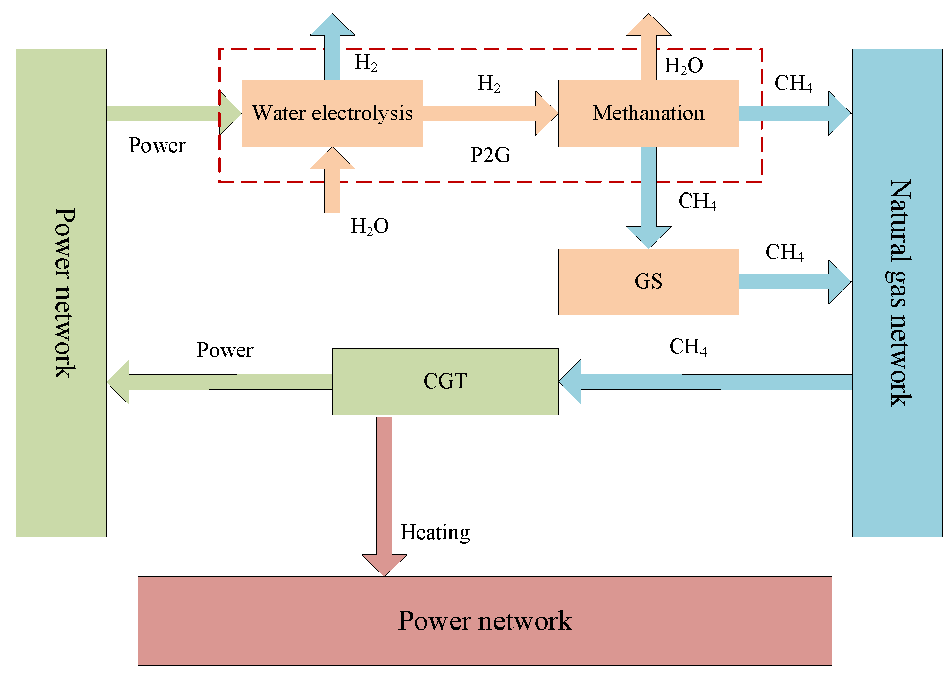
| P2G | power-to-gas |
| P2C | power to cooling |
| P2H | power to heating |
| H2C | heating to cooling |
| GS | gas storage tank |
| PS | power storage battery |
| HS | heat storage tank |
| CS | cold storage tank |
| DR | demand response |
| PBDR | price-based demand response |
| IBDR | incentive-based demand response |
| EP | energy production |
| EC | energy conversion |
| ES | energy storage |
| FET | following electric load |
| FTL | following thermal load |
| Set | |
| t, s | index for time |
| k | index for energy type |
| j | index for step |
| Parameter | |
| rated power of WPP | |
| cut-in speed | |
| rated speed | |
| cut-out speed | |
| conversion productivity | |
| receiving light of PV | |
| natural gas calorific value | |
| operation efficiency of CGT at time t | |
| radiation intensity at time t | |
| real-time speed at time t | |
| initial load before PBDR. at time t | |
| energy use efficiency of EC and ES | |
| energy supply efficiency of EC and ES | |
| loss rate of ES at time t | |
| Variables | |
| power supply of CGT at time t | |
| heating supply of CGT at time t | |
| gas consumption at time t | |
| cooling power produced by P2C at time t | |
| heating power from P2H at time t | |
| cooling power from H2C at time t | |
| electricity consumption of P2C at time t | |
| electricity consumption of P2H at time t | |
| heating consumption of H2C at time t | |
| energy storage of ES at time t | |
| Input power of ES at time t | |
| output power of ES at time t | |
| price variable after PBDR at time s | |
| load variable after PBDR at time s | |
| output power of energy k provided by IBDR at time t | |
| operation revenue of EP at time t | |
| operation revenue of EC at time t | |
| operation revenue of ES at time t | |
| operation revenue of DR at time t | |
| carbon trading revenue at time t | |
| fuel consumption cost of CGT at time t | |
| start-stop cost of CGT at time t | |
| start-up and shut-down state variable at time t | |
| power output of CGT at time t | |
| heating output of CGT at time t | |
| start-up state variable of CGT at time t | |
| downhill power limits of CGT | |
| uphill power limits of CGT | |
| operating status of the CGT | |
| state variables of EC outputting energy at time t | |
| load forecast deviation at time t | |
| system net load demand | |
| maximum output of DRP i in step j providing energy k | |
| minimum response output of DRP i in step j providing energy k | |
| actual load reduction value of energy k that DRP i provides in j step at time t | |
| available load reduction value of energy k that DRP i can provides in step j at time t | |
| electric-thermal conversion coefficient of CGT | |
| power supply cost coefficient of CGT | |
| energy price before PBDR at time t | |
| energy price after PBDR at time t | |
| , , | carbon emission coefficient of the CGT |
| , | value of c with the minimum and maximum output power |
| maximum heating power of CGT | |
| heating supply power of the turbine when electricity power supply of CGT is minimum | |
| , | maximum and minimum power generation of CGT under pure condensation |
| , | minimum and maximum gas production power of P2G |
| , | upper and lower limits of EC energy supply |
| , e | upper and lower limits of EC energy consumption |
| , | minimum and maximum energy storage of ES at time t |
| , | minimum and maximum of ES energy supply at time t |
| , | minimum and maximum limits of ES energy consumption at time t |
| , | up-rotating reserve coefficients of electricity and cooling load |
| , | up-rotating reserve coefficients of WPP and PV |
| , | down-rotating reserve coefficients of WPP and PV |
| , | maximum and minimum power supply at time t |
| E, | shape and scale parameter |
| , | shape parameters of the Beta distribution |
| heat recovery efficiency | |
| energy conversion efficiency of P2C, | |
| capacity loss rate | |
| energy conversion efficiency of P2H | |
| energy conversion efficiency of H2C | |
| energy storage efficiency | |
| energy release efficiency | |
| energy demand price elasticity matrix | |
| maximum output power of PV at time t | |
| available power of WPP at time t | |
| shut-down state variable of CGT at time s | |
| start-up cost at time t | |
| hut-down cost of CGT at time s + 1 | |
| output energy of EC and ES at time t | |
| input energy of EC and ES at time t | |
| energy use price of EC and ES | |
| energy supply price of EC and ES | |
| energy demand after PBDR at time t | |
| shortage of energy k at time t | |
| energy supply price of IBDR at time t | |
| real-time energy supply price of energy k at time t | |
| Maximum MTEA at time t | |
| carbon market transaction price at time t | |
| energy of MEG bought from the upper power grid at time t | |
| energy of MEG bought from the upper heating grid at time t | |
| energy of MEG bought from the upper cooling grid at time t | |
| power consumption of P2G at time t | |
| power generation of P2G at time t | |
| power consumption of P2H at time t | |
| power consumption of P2C at time t | |
| power generation output provided by PBDR at time t | |
| power generation output provided by IBDR at time t | |
| heating power of H2C at time t | |
| heating storage of HS at time t | |
| heating release of HS at time t | |
| consumption of heating of H2C at time t | |
| heating output power provided by PBDR at time t | |
| heating output power provided by IBDR at time t | |
| cooling output of P2C at time t | |
| cooling output of H2C at time t | |
| cooling storage of CS at time t | |
| cooling release of CS at time t | |
| cooling output power provided by PBDR at time t | |
| cooling output power provided by IBDR at time t | |
| state variables of EC inputting energy at time t | |
| state variables of ES outputting energy at time t | |
| state variables of ES inputting energy at time t | |
| electric power of MEG at time t | |
| load demand forecast value at time t | |
References
- Rifkin, J. The Third Industrial Revolution: How Lateral Power is Transforming Energy, the Economy, and the World; St. Martin’s Press: New York, NY, USA, 2011. [Google Scholar]
- Guidance on Promoting the Development of "Internet +" Smart Energy. Available online: https://kns.cnki.net/KCMS/detail/detail.aspx?dbcode=CJFQ&dbname=CJFDLAST2016&filename=CSYQ201604001&v=MTgxNTZyV00xRnJDVVJMT2VaZVpzRnluaFZidlBKajdTZjdHNEg5Zk1xNDlGWllSOGVYMUx1eFlTN0RoMVQzcVQ=) (accessed on 4 November 2019).
- Liu, Y.B.; Zuo, K.Y.; Liu, X.W. Dynamic pricing for decentralized energy trading in micro-grids. Appl. Energy 2018, 228, 689–699. [Google Scholar] [CrossRef]
- Rossi, I.; Banta, L.; Cuneo, A.; Ferrari, M.L.; Traverso, A.N.; Traverso, A. Real-time management solutions for a smart polygeneration microgrid. Energy Convers. Manag. 2016, 112, 11–20. [Google Scholar] [CrossRef]
- Dong, W.L.; Wang, Q.; Yang, L. A coordinated dispatching model for distribution utility and virtual power plants with wing/photovoltaic/hydro generators. Autom. Electr. Power Syst. 2015, 39, 75–82. [Google Scholar]
- Yu, S.; Wei, Z.H.; Sun, G.Q. A bidding model for a virtual power plant considering uncertainties. Autom. Electr. Power Syst. 2014, 38, 44–49. [Google Scholar]
- Liu, X.Y. Research on Performance of Combined Heating System of Solar Energy and Electric Boiler, North China Electric Power University. 2017. Available online: https://kns.cnki.net/KCMS/detail/detail.aspx?dbcode=CMFD&dbname=CMFD201801&filename=1017222760.nh&v=MTE4NzJGeW5oVnIzQlZGMjZHYkc2SE5iS3I1RWJQSVI4ZVgxTHV4WVM3RGgxVDNxVHJXTTFGckNVUkxPZVplWnM= (accessed on 4 November 2019).
- Mengdong Power Wind Power Heating Pilot 3 Years to Reduce Coal Consumption by 68,700 Tons. Polaris Power Network. 7 November 2016. Available online: http://www.sohu.com/a/118288979_131990 (accessed on 7 November 2016).
- Zhang, X.; Yang, J.H.; Wang, W.Z. Integrated optimal dispatch of a rural micro-energy-grid with multi-energy stream based on model predictive control. Energies 2018, 11, 3439. [Google Scholar] [CrossRef]
- Du, L.; Sun, L.; Chen, H.H. Multi-index evaluation of integrated energy system with P2G planning. Electr. Power Autom. Equip. 2017, 37, 110–116. [Google Scholar]
- Luo, Y.H.; Yin, Z.X.; Yang, D.S. A new wind power accommodation strategy for combined heat and power system based on bi-directional conversion. Energies 2019, 12, 2458. [Google Scholar] [CrossRef]
- Peik-Herfeh, M.; Seifi, H.; Sheikh-El-Eslami, M.K. Decision making of a virtual power plant under uncertainties for bidding in a day-ahead market using point estimate method. Int. J. Elec. Power 2013, 44, 88–98. [Google Scholar] [CrossRef]
- Yang, H.M.; Yi, D.X.; Zhao, J.H. Distributed optimal dispatch of virtual power plant based on ELM transformation. Management 2014, 10, 1297–1318. [Google Scholar] [CrossRef]
- Zamani, A.G.; Zakariazadeh, A.; Jadid, S. Day-ahead resource scheduling of a renewable energy based virtual power plant. Appl. Energy 2016, 169, 324–340. [Google Scholar] [CrossRef]
- Tan, Z.F.; Wang, G.; Ju, L.W. Application of CVaR risk aversion approach in the dynamical scheduling optimization model for virtual power plant connected with wind-photovoltaic-energy storage system with uncertainties and demand response. Energy 2017, 124, 198–213. [Google Scholar] [CrossRef]
- Hu, M.C.; Lu, S.Y.; Chen, Y.H. Stochastic programming and market equilibrium analysis of microgrids energy management systems. Energy 2016, 113, 662–670. [Google Scholar] [CrossRef]
- Tsao, Y.C.; Thanh, V.V.; Lu, J.C. Multiobjective robust fuzzy stochastic approach for sustainable smart grid design. Energy 2016, 176, 929–939. [Google Scholar] [CrossRef]
- Li, Z.M.; Xu, Y. Temporally-coordinated optimal operation of a multi-energy microgrid under diverse uncertainties. Appl. Energy 2019, 240, 719–729. [Google Scholar] [CrossRef]
- Ju, L.W.; Tan, Q.L.; Zuo, X.T.; Zhao, R. A risk aversion optimal model for microenergy grid low carbon-oriented operation considering power-to-gas and gas storage tank. Int. J. Energy Res. 2019, 43, 1–20. [Google Scholar] [CrossRef]
- Chen, Y.; Wei, W.; Liu, F. Analyzing and validating the economical efficiency of managing a cluster of energy hubs in multi-carrier energy systems. Appl. Energy 2018, 230, 403–416. [Google Scholar] [CrossRef]
- Ju, L.W.; Zhao, R.; Tan, Q. A multi-objective robust scheduling model and solution algorithm for a novel virtual power plant connected with power-to-gas and gas storage tank considering uncertainty and demand response. Appl. Energy 2019, 250, 1336–1355. [Google Scholar] [CrossRef]
- Wang, G.; Tan, Z.F.; Lin, H.Y. Multi-level market transaction optimization model for electricity sales companies with energy storage plant. Energies 2019, 12, 145. [Google Scholar] [CrossRef]
- Liu, F.; Zhang, K.L.; Zou, R.M. Robust LFC strategy for wind integrated time-delay power system using EID compensation. Energies 2019, 12, 3223. [Google Scholar] [CrossRef]


| Energy Production/kW·h | Energy Conversion/kW·h | ||||||
| WPP | PV | Conventional gas turbine (CGT) | Power-to-heat (P2H) | Power-to-gas (P2G) | Power-to-cooling (P2C) | Heat-to-cooling (H2C) | |
| Power | 10,731 | 7027 | 35,674 | −1967 | −2623 | −14,649 | - |
| Heating | - | - | 57,600 | 1869 | - | - | −10,724 |
| Cooling | - | - | - | - | - | 43,946 | 14,477 |
| Energy Storage/kW·h | Gas storage tank (GST) | Revenue/¥ | Carbon/ton | CVaR/¥ | |||
| Power storage (PS) | Heat storage (HS) | Cooling storage (CS) | |||||
| Power | ±2400 | - | - | 1129 | 14,882.59 | 1.95 | - |
| Heating | - | ±2400 | - | - | 21,474.53 | 2.45 | - |
| Cooling | - | - | ±3600 | - | 11,180.93 | - | - |
| Energy Production/kW·h | Energy Storage/kW·h | GST | |||||
| WPP | PV | CGT | PS | HS | CS | ||
| Power | 10,166 | 6657 | 35,674 | ±2400 | - | - | 814 |
| Heating | - | - | 57,600 | - | ±2400 | - | - |
| Cooling | - | - | - | - | - | ±3600 | - |
| Energy Conversion/kW·h | Revenue/¥ | Carbon/ton | CVaR/¥ | ||||
| P2H | P2G | P2C | H2C | ||||
| Power | −2231 | −1223 | −14,536 | - | 14,268.502 | 2.25 | 9702.581 |
| Heating | 2091 | - | - | −10,947 | 21,555.33 | 2.68 | 9268.792 |
| Cooling | - | - | 43,607 | 14,778 | 11,324.708 | - | 3284.165 |
| WPP | PV | CGT | UPG | Revenue/¥ | Carbon/ton | CVaR/¥ | ||
|---|---|---|---|---|---|---|---|---|
| Power | Heating | |||||||
| 0 | 10,731.2 | 7027.15 | 35,673.6 | 57,600 | ±1647.83 | 47,538.051 | 4.4 | 0 |
| 0.5 | 10,668.26 | 6998.85 | 35,673.6 | 57,600 | ±1745.25 | 47,493.781 | 4.46 | 6152.16 |
| 0.6 | 10,542.38 | 6942.25 | 35,673.6 | 57,600 | ±1945.24 | 47,405.24 | 4.58 | 18,456.48 |
| 0.7 | 10,354.39 | 6799.776 | 35,673.6 | 57,600 | ±2207.525 | 47,276.89 | 4.755 | 20,356.01 |
| 0.8 | 10,166 | 6657 | 35,673.6 | 57,600 | ±2469.81 | 47,148.54 | 4.93 | 22,255.54 |
| 0.9 | 10,026.13 | 6377.767 | 35,673.6 | 57,600 | ±2685.12 | 46,391.147 | 5.26 | 23,729.51 |
| 1.0 | 9956 | 6238 | 35,673.6 | 57,600 | ±2845.85 | 46,012.45 | 5.43 | 24,466.5 |
| Energy Production/kW·h | Energy Storage/kW·h | GST | |||||
| WPP | PV | CGT | PS | HS | CS | ||
| Power | 9602 | 6287 | 35,674 | ±2400 | - | - | 153 |
| Heating | - | - | 57,600 | - | ±2400 | - | - |
| Cooling | - | - | - | - | - | ±3300 | - |
| Energy Conversion/kW·h | Revenue/¥ | Carbon/ton | CVaR/¥ | ||||
| P2H | P2G | P2C | H2C | ||||
| Power | −73 | −230 | −16,091 | - | 13,398.987 | 2.47 | 8709.342 |
| Heating | 70 | - | - | −7586 | 21,464.787 | 2.83 | 9229.858 |
| Cooling | - | - | 48,273 | 10,241 | 11,581.694 | - | 4053.593 |
| PBDR | WPP | PV | CGT | Energy Storage/kW·h | |||
| Power | Heating | PS | HS | CS | |||
| Before | 9602 | 6287 | 35,674 | 57,600 | ±2400 | ±1800 | ±3000 |
| After | 10,167 | 6657 | 35,674 | 57,600 | ±1800 | ±2400 | ±3600 |
| PBDR | GST | IBDR | Revenue/¥ | Carbon/ton | CVaR/¥ | ||
| Power | Heating | Cooling | |||||
| Before | 153 | - | - | - | 46,445 | 5.30 | 21,993 |
| After | 86 | ±1200 | ±1000 | ±1200 | 50,935 | 4.60 | 22,189 |
| META | WPP | PV | IBDR | ES | Carbon Emission/ton | Revenue/103¥ | CVaR/103¥ | ||||
|---|---|---|---|---|---|---|---|---|---|---|---|
| Power | Heating | Cooling | Power | Heating | Cooling | ||||||
| 60% | 11,258 | 7045 | ±1600 | ±1300 | ±1500 | ±2400 | ±3000 | ±3900 | 55,688.93 | 3.45 | 27,854 |
| 70% | 11,085 | 6842 | ±1400 | ±1200 | ±1300 | ±1800 | ±3000 | ±3900 | 53,554.51 | 4.03 | 25,358.86 |
| 80% | 10,167 | 6657 | ±1200 | ±1000 | ±1200 | ±1800 | ±2400 | ±3600 | 50,935 | 4.60 | 22,189 |
| 90% | 9650 | 6245 | ±1100 | ±800 | ±900 | ±1800 | ±1800 | ±3000 | 47,539.33 | 5.18 | 19,723.56 |
| 100% | 9325 | 6018 | ±900 | ±700 | ±900 | ±1200 | ±1800 | ±3000 | 44,822.8 | 5.75 | 17,751.2 |
© 2019 by the authors. Licensee MDPI, Basel, Switzerland. This article is an open access article distributed under the terms and conditions of the Creative Commons Attribution (CC BY) license (http://creativecommons.org/licenses/by/4.0/).
Share and Cite
Fu, X.; Fan, W.; Lin, H.; Li, N.; Li, P.; Ju, L.; Zhou, F. A Risk Aversion Dispatching Optimal Model for a Micro Energy Grid Integrating Intermittent Renewable Energy and Considering Carbon Emissions and Demand Response. Processes 2019, 7, 916. https://doi.org/10.3390/pr7120916
Fu X, Fan W, Lin H, Li N, Li P, Ju L, Zhou F. A Risk Aversion Dispatching Optimal Model for a Micro Energy Grid Integrating Intermittent Renewable Energy and Considering Carbon Emissions and Demand Response. Processes. 2019; 7(12):916. https://doi.org/10.3390/pr7120916
Chicago/Turabian StyleFu, Xiaoxu, Wei Fan, Hongyu Lin, Nan Li, Peng Li, Liwei Ju, and Feng’ao Zhou. 2019. "A Risk Aversion Dispatching Optimal Model for a Micro Energy Grid Integrating Intermittent Renewable Energy and Considering Carbon Emissions and Demand Response" Processes 7, no. 12: 916. https://doi.org/10.3390/pr7120916
APA StyleFu, X., Fan, W., Lin, H., Li, N., Li, P., Ju, L., & Zhou, F. (2019). A Risk Aversion Dispatching Optimal Model for a Micro Energy Grid Integrating Intermittent Renewable Energy and Considering Carbon Emissions and Demand Response. Processes, 7(12), 916. https://doi.org/10.3390/pr7120916