
Article

Staged Effective Medium Modeling and Experimental Validation for Rock Thermal Conductivity
Rock Mechanics, Petrophysics and Sample Characterization Laboratory, Department of Petroleum Engineering, University of Houston, Houston, TX 77204, USA
*
Author to whom correspondence should be addressed.
Processes 2026, 14(9), 1437; https://doi.org/10.3390/pr14091437
Submission received: 11 February 2026 / Revised: 10 April 2026 / Accepted: 23 April 2026 / Published: 29 April 2026

Abstract

The thermal conductivity (λ) of porous rocks as a function of total porosity, grain size, and fluid saturation is measured and modeled by combining high-precision experiments with a Staged Differential Effective Medium (SDEM) modeling framework. A 1-D divided-bar apparatus with computer-controlled guard heaters with an integrated ultrasonic pulse-transmission system was developed to measure the thermal conductivity and P and S-wave velocities simultaneously. Measurements were made on Fontainebleau sandstone cores and quartz sand packs of varying grain size and effective stresses up to 2000 psi. The sample properties were measured in both dry and water-saturated states. The SDEM model performs significantly better at predicting the saturated thermal conductivities in the sand packs. For the sand packs, the thermal conductivity and compressional velocity are the highest and most stress-sensitive for the fine-grained material. In contrast, the shear velocity is largest in the coarse-grained material. The SDEM model is adapted from previous acoustic models for use in understanding thermal conductivity. These joint models accurately reproduce the evolution of both thermal conductivity and bulk modulus during increasing compaction and varying saturation. A single parameter fits both the dry and saturated data, which allows Gassmann-style fluid substitution for the thermal conductivity. This model improves the prediction of in situ thermal conductivity from sonic well logs.

1. Introduction

  • Motivation
The thermal conductivity of rocks is defined as the ability of the material to conduct heat, or the rate of heat transfer through a unit area under a unit temperature gradient (W·m−1·K−1), which is a key parameter in geoscience and engineering that governs heat transfer [1]. Thermal conductivity controls geothermal gradients, energy transport in reservoirs and repositories, and heat dissipation in tunnels, foundations, and buried infrastructure [2,3]. Geothermal energy relies on extracting subsurface heat; the thermal conductivity of the host rocks directly determines the efficiency of heat flow toward production wells and thus the sustainability and power potential of geothermal systems [4,5,6]. Typical thermal conductivities of sedimentary formations span approximately 1–6 W·m−1·K−1, reflecting substantial lithological variability: from high-conductivity quartz-rich rocks (~7.7 W·m−1·K−1) to low-conductivity clay-rich units (~2 W·m−1·K−1) [7,8]. The commonly used thermal conductivity of natural quartz is ~7.7 W·m−1·K−1 [2,8]. However, when field and lab data are extrapolated to zero porosity in quartz-rich sandstones, it typically falls below this value due to the influence of lower thermal conductivity minerals, thermal contact resistance at grain boundaries, the assumption of perfect grain packing at zero porosity, and the exclusion of the influence of micropores and cements. Such variability introduces significant uncertainty into geothermal and heat flow modeling, as even modest deviations in thermal conductivity can markedly influence subsurface temperature predictions. Consequently, recent investigations underscore the need to accurately constrain thermal conductivity distributions to improve the reliability of modeled geothermal gradients and subsurface thermal regimes [9,10].
  • Borehole-Based Measurements
In situ determinations can be performed using downhole thermal conductivity logging tools [4,11,12,13]. These measurements are typically spatially discontinuous, technically demanding, and economically restrictive. In shallow subsurface investigations, the thermal response test (TRT) has become a widely adopted technique for assessing the effective thermal properties of borehole environments [14]. For deeper boreholes, optical frequency-domain reflectometry (OFDR) enables direct, high-resolution profiling of thermal conductivity along the borehole wall [15]. Measurements in unconsolidated sediments require controlled variation in water content and the application of incremental compaction pressures to account for the strong dependence of heat transfer on fluid saturation and packing density [16]. These methods have led to wide variations in the values of thermal conductivity measurements, which inhibit model calibration and increase prediction errors in modeling subsurface heat flow [17].
  • Laboratory Measurements
Laboratory thermal conductivity measurements are broadly classified into steady-state and transient-state methods, depending on whether a constant or time-dependent temperature gradient is imposed across the sample [1,17]. Steady-state techniques, such as the divided-bar and guarded-hot-plate methods, determine thermal conductivity once thermal equilibrium is achieved, yielding high accuracy but requiring longer equilibration times and precise control of boundary conditions [18]. In contrast, transient methods, including the line-source (needle probe) and laser-flash techniques, infer conductivity from the dynamic temperature response to a heat pulse or step input, allowing for faster measurements and application to a broader range of materials [17,19]. Steady-state methods are limited by sample geometry constraints and susceptibility to heat losses, while transient methods are affected by uncertainties in contact resistance, heat capacity estimation, and assumptions of homogeneity [20,21]. Often, datasets are obtained using diverse experimental setups and methodological approaches [16]. Datasets are reported inconsistently, as some studies report only median values, while others provide full ranges or extreme bounds (minimum and maximum) with an uncertainty range of approximately 5–50% [16]. In addition, this variability in thermal conductivity values reflects the influence of the microstructural and saturation properties of the rock [22]. These differences in data reporting and measurement techniques preclude rigorous statistical analysis.
  • Correlations
In attempts to understand this variability in the measurements, a substantial body of research has employed empirical mixing laws to estimate the effective thermal conductivity of rocks from petrophysical parameters. In two-phase systems comprising a solid matrix and pore space, the simplest theoretical limits are provided by the Wiener bounds [23], which represent end-member limits in which heat flow is either parallel or perpendicular to bedding. Numerous studies have used indirect methods for estimating thermal conductivity from petrophysical parameters such as bulk density, porosity, and mineralogical composition [24,25,26]. These regression-based empirical formulations are inherently limited, as their validity is generally restricted to the specific lithologies and environmental conditions for which they were calibrated. Comprehensive summaries are provided in [24].
  • Empirical Models
These predictive uncertainties in the bulk thermal conductivity of a rock are governed by its mineralogical composition, porosity, pore fluid characteristics, and the geometric configuration of its pore network. Sandstones, shales, and carbonates with comparable bulk compositions may nonetheless exhibit distinctly different thermal conductivities due to variations in pore structure and connectivity [27]. In particular, the presence of anisotropic pore systems and microcrack networks can enhance or inhibit heat transfer depending on their orientation relative to the thermal gradient [20,24]. Furthermore, fluid saturation exerts a strong influence, as the substitution of air by water or brine substantially increases the effective thermal conductivity through improved heat transfer across pore spaces [4,8,28]. The application of induced stress closes microcracks and increases grain-to-grain contact areas, enhancing heat transfer efficiency and improving thermal conductivity [29]. Temperature exerts an opposite effect on thermal conductivity: higher temperatures enhance phonon scattering, intensifying lattice vibrations and disrupting the orderly transfer of thermal energy through the crystal lattice, thereby diminishing effective heat transport [30,31]. In porous, fluid-saturated rocks, temperature-induced changes in fluid properties (e.g., density) may partially counteract this reduction by improving conductive pathways within the pore network [4,20]. Consequently, accurate modeling requires applying temperature-dependent corrections to measured thermal conductivity to obtain precise estimates of subsurface heat flow. These interrelated thermal effects highlight the importance of integrating mineralogical, textural, geomechanical, and petrophysical parameters to predict the thermal properties of geological formations in geothermal systems and basin-scale heat flow models [30,31,32].
  • Bounds
Attempts to reduce this uncertainty have been improved by establishing bounds on the possible values of the thermal conductivity. For isotropic media, the Hashin–Shtrikman bounds provide the most restrictive theoretical limits [33]. Between the Wiener and Hashin–Shtrikman bounds, various rock physics models have been applied to estimate an “effective” thermal conductivity of rocks. The Maxwell–Eucken models provide two complementary formulations for heat transfer in rocks, distinguishing whether the solid matrix or the pore fluid forms the continuous phase containing isolated spherical inclusions [34,35,36]. Both models rely on dilute-sphere assumptions in which inclusions are non-interacting and randomly distributed, making them most valid at low porosity where phase interactions remain negligible. Although simple, they offer only first-order estimates of effective thermal conductivity, but they underpin more advanced effective medium theories commonly used in geothermal and basin-scale heat flow modeling [8,24]
  • Self-Consistent Models
An example of a self-consistent formulation is Bruggeman’s widely used symmetrical effective medium model that predicts composite thermal conductivity by treating both the solid and fluid phases as statistically equivalent constituents embedded within an infinite surrounding medium. This approach incorporates higher inclusion concentrations and phase-interaction effects, yielding more realistic bulk thermal conductivity estimates in heterogeneous or isotropic materials [24,31]. Differential Effective Medium models composite behavior by incrementally introducing inclusions into a uniform host and updating the effective properties at each step. This enables modeling the thermal conductivity of mixtures more realistically than static mixing laws [37,38]. Although DEM models often yield improved predictions for rocks with moderate porosity or anisotropy, they may diverge from observed thermal conductivities when microstructural heterogeneity or fabric orientation strongly control heat transport [24,39]. The geometric mean model [40] estimates bulk thermal conductivity as the geometric average of the matrix and pore conductivities, weighted by their volume fractions, assuming an isotropic, randomly distributed two-phase system. Although it lacks explicit microstructural parameters, it often matches the performance of more complex EMT formulations for consolidated rocks with moderate porosity. This typically predicts sandstone thermal conductivity within about ten to twenty percent [8]. Other studies show that weighted geometric means often provide the best empirical fits to laboratory data [41]. More sophisticated models yield only marginal improvements [3,42]. Zimmerman modified the Hashin–Shtrikman upper bound by incorporating a textural parameter, namely, the pore aspect ratio, which directly influences the distribution of heat flow paths [43].
  • Pore Structure-Based Models
Pimienta et al. developed effective medium theory-based models to predict thermal conductivity in porous and microcracked rocks by explicitly incorporating crack density and aspect ratio into the upscaling scheme [44]. Model 2 embeds compliant cracks into a high-pressure host medium, assuming all cracks are closed, reducing assumptions about mineralogy and pore shape and enabling more reliable inversion of crack parameters as pressure decreases. In contrast, Model 3 assumes a monomineralic matrix with spherical, stress-insensitive pores and uses the Mori–Tanaka homogenization scheme, introducing additional assumptions and generating larger uncertainties in predicted crack geometry and thermal conductivity. The authors also show that although thermal conductivity can be reasonably inferred from elastic wave velocity and porosity, the predictions remain limited by assuming a simplified pore geometry, idealized microstructural assumptions, and the inherent non-uniqueness of the inverse crack-parameter problem. These models offer useful theoretical constraints on thermal conductivity, but none adequately capture the complexity of natural rocks [3,42]. This level of uncertainty implies that improved links to other readily measured parameters are needed.
  • Joint Modeling of Modulus and Thermal Conductivity
Elastic-wave velocity in rocks exhibits similar sensitivity to mineral composition, porosity, fluid saturation, and fabric anisotropy as thermal conduction, and seismic velocity measurements are often employed as indirect proxies for estimating thermal conductivity [45]. Empirical relationships between thermal conductivity and P-wave velocity (Vp) have been established for specific lithologies, indicating that for dry sandstones and volcanites, thermal conductivity can be estimated from Vp with an accuracy of approximately ±0.5 W·m−1·K−1 [28]. They also showed that increasing water saturation leads to simultaneous increases in both thermal conductivity and P-wave velocity, with porosity exerting a dominant influence on the strength of this relationship. However, Mielke et al. reported weak correlations between thermal conductivity and P-wave velocity in clastic sediments, as evidenced by low coefficients of determination (R2 = 0.04–0.48) across sandstone types [28]. This indicates that acoustic velocity alone provides only limited predictive capability for thermal conductivity, reflecting the complex influence of porosity, mineralogy, and microstructural heterogeneity. Subsequent investigations have proposed linear and non-linear empirical correlations between these properties. Such models remain largely statistical in nature and lack explicit physical grounding [46]. Several studies have explored the interdependence of thermal conductivity and elastic-wave velocity through their mutual sensitivity to porosity, mineralogy, fluid saturation, and confining stress [47,48]. These approaches rely primarily on direct regression between velocity and thermal conductivity.
  • Staged Differential Effective Medium Models (SDEM models)
As described above, the classical mixing laws and conventional effectivemedium formulations show systematic biases and fail to capture detailed mineralogical and fabric effects. The SDEM technique allows interpolation between Voight and Reuss bounds and also allows varying minerals and porosity changes to be included through multiple integration stages using a Differential Effective Medium approximation. This modeling technique has been extensively validated for acoustic moduli and resistivity [49,50,51,52]. An important contribution of this type of modeling is the development and validation of a Staged Differential Effective Medium (SDEM) model that accurately predicts effective thermal conductivity (ETC). This model allows fluid substitution similar to a Gassman substitution, which provides an important validation of the modeling and the measurement capabilities.
Two systems were investigated, a lithified sandstone, Rupelian Fontainebleau (Young’s modulus ~106), with porosity varying between 9% and 12%, and low modulus (~50 × 103) sand packs with varying porosity (between 17% and 37%) due to different levels of compaction. Both rock types are quartz-dominated but with different fabric geometries.

2. Materials and Methods

A custom-designed, calibrated, divided-bar 1-D system for high-precision thermal conductivity measurements of small cylindrical rock discs, equipped with multiple computer-controlled guard heaters, was developed. The samples are confined between two heated reference samples in a 1-D axial setup, which minimizes any buoyancy-driven circulation. The thermal conductivity apparatus and pulse-transmission ultrasonic setup were then used to measure thermal conductivity and acoustic velocities under increasing isostatic stress (200–2000 psi) for Fontainebleau sandstones and laboratory-constructed sand packs (of varying grain size and mineralogy) in both dry and saturated states.

2.1. Sample Description and Preparation

Two different sample sets, Fontainebleau sandstone and Brazos River sand packs, were chosen to reflect a common mineralogy (quartz dominated) but different porosities and levels of cementation. The sand packs allowed a range in grain sizes and porosities to be generated.

2.1.1. Fontainebleau Sandstone

The Rupelian Fontainebleau sandstone, deposited in a marine shoreface subaerial–eolian environment, is quartz-rich (quartz > 99%) and known for its high degree of cementation and uniform grain fabric [53]. Three cylindrical cores (2.54 cm in diameter and ~6 cm in length) were drilled from large rectangular blocks using a water-cooled diamond-tipped coring bit. The samples were precision-ground and polished at both ends (right cylindrical geometry) to ensure good thermal contact for thermal conductivity measurements and reliable coupling of acoustic transducers to the samples. The core plugs were vacuum-oven-dried at 60 °C. The dry weight, bulk volume, and dry bulk density were measured using calipers and a precision balance. Grain density and porosity were determined using a nitrogen expansion (Boyle’s Law) porosimeter. The samples were saturated by evacuating for one hour, followed by the injection of degassed water. The sample then remained at 800 psi pressure for 12 h to ensure full saturation.

2.1.2. Sand Packs

The sand-pack specimens were prepared from Brazos River sand, which is quartz-rich and characterized by subangular grains.
As shown in Table 1, three grain-size fractions (45–75 μm, 180–212 μm, and 355–425 μm) were prepared by sieving to ensure consistent particle-size distributions. Samples were sleeved in heat-shrink Viton (2.5 cm inner diameter and ~3 cm length). The initial porosity was almost independent of grain size. This allows direct grain size comparisons.
A series of isostatic compaction experiments were performed on the 355–425 μ m sand to produce a wide range of porosities for testing. Both thermal conductivity and ultrasonic wave velocities were measured in both dry and saturated states. After compaction, the sample porosity is given by:
ϕ f i n a l = 1 ( 1 ϕ i n i ) l i n i l f i n a l
where ϕ i n i is the initial porosity (fraction), ϕ f i n a l is the porosity after compaction, l i n i is the initial sample length, and l f i n a l is the final sample length (after compaction). The calculation assumes that the grain volume is constant.

2.2. Thermal Conductivity (λ) Measurement and Calibration

2.2.1. Measurement

A steady-state divided-bar apparatus, integrated with a servo-controlled pressure vessel, was used to measure thermal conductivity. The apparatus combines two subsystems: (1) a divided-bar thermal conductivity assembly with actively tuned guard heaters across a 1-inch diameter sample column and (2) a triaxial press employing a programmable isostatic pressure (+1% error) to the sample stack (Figure 1). The core sample was placed between two high-thermal-conductivity aluminum discs (Figure 1). A constant heat flux was applied to the top disc by an electric heater, while the bottom disc was held at a lower reference temperature (Figure 1). The temperature drop across the sample was measured by precision RTD sensors embedded in the aluminum discs, and a one-dimensional Fourier’s law (steady state) was used to compute the sample’s thermal conductivity (Figure 2). This divided-bar stack consists of (in order): a heat source (temperature-controlled bath or heater), an upper heat flow meter (aluminum disc), the rock sample, a lower heat flow meter, and a heat sink [54]. The stack was surrounded by thermal insulation to minimize convective heat losses. Guard heaters were applied to eliminate radial heat flow.
The improved divided-bar apparatus uses three independently PID (Proportionality–Integral–Derivative)-controlled guard heaters (two for the reference sections and one for the sample) to minimize radial heat losses. The error signal for the steady-state control condition is determined by the temperature gradients across the standards:
e t = G t o p G b o t t o m
where e t is the input error signal, and G t o p and the G b o t t o m terms are the measured temperature gradients across the top and bottom standards. The error signal measures the imbalance in heat flow. The time-discretized PID for the top and bottom sections is based on the PID control, u(t), and is adjusted to supply heat flux as:
u t = K p e K + K I T S I = 0 k e i + K d e k e k 1 T s
where e K is the current error at time step K, i.e., the difference between the target gradient (setpoint) and the measured gradient, K p e K is the proportional error term, which applies a correction proportional to the errors (in response to deviations), K I T S I = 0 k e i is the integral term, which accumulates past errors to eliminate steady-state offsets, T s is the sampling time (time interval between control updates), and K d e k e k 1 T s is the derivative term, which anticipates future error trends by estimating the rate of change in error, which helps to dampen oscillations. The proportional, integral, and derivative gains ( K p , K I , K d ) tune the responsiveness, stability, and smoothness of temperature control. The middle (sample) section’s heater power is modeled and balanced in the divided-bar thermal conductivity apparatus using Newton’s law of cooling to account for radial heat loss across the sample:
= α T c T e n v = α T
where is the radial heat flux lost from the sample to the environment, not the main conductive heat passing through the stacked setup, α is the heat transfer coefficient, T c is the surface temperature of the middle section, and T e n v is the ambient temperature. The term α T quantifies radial heat losses for each section. The proportionality expresses how radial heat losses from each section of the divided-bar apparatus relate to their local temperature differences (ΔT) and are assumed equal. The equilibrium in the mid-section power ( P mid ) is assumed to be the average of the top and bottom sections.
P m i d = m i d = t o p T m i d T t o p + b o t t o m T m i d T b o t / 2 .
This corrects for heat losses in the mid-section by maintaining constant axial heat flux through the top and bottom standards.
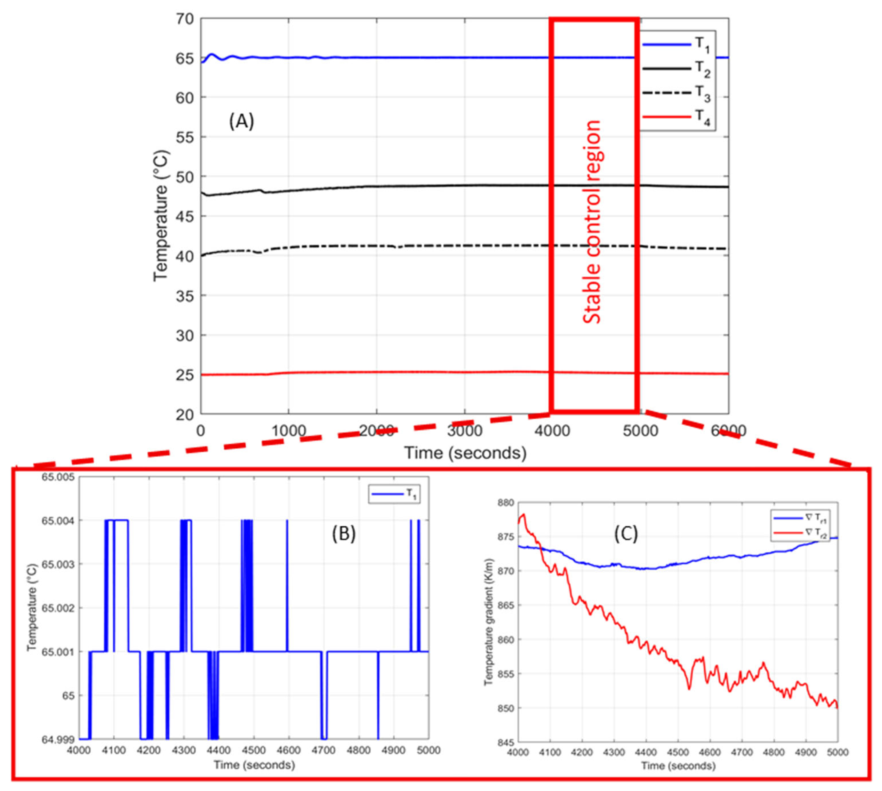
The measurement stack is illustrated in Figure 1. The standard gradients are calculated between T1 and T2 (upper gradient) and T3 and T4 (lower gradient), and between T2 and T3 (the sample gradient). A fused quartz standard sample was used for the PID-controlled heater calibration. Figure 2 shows an example of the time-dependent evolution of the temperature for the four thermocouples monitored over a 6000 s interval, where T1 (blue) corresponded to the top aluminum section maintained at approximately 65 °C, T2 (solid black) to the upper reference standard near 48 °C, T3 (black dashed) to the sample region around 41 °C, and T4 (red) to the bottom aluminum section stabilized near 25 °C. All temperatures reach a steady state between 4000 and 5000 s after an initial transient, indicating excellent thermal stability (Figure 2A). The small fluctuations (<0.01 °C) suggest that the PID controllers are maintaining a nearly constant temperature with minimal oscillation, which is a key condition for accurate steady-state thermal conductivity measurement. The zoomed-in view of T1 between 4000 and 5000 s shows variations within ±0.0025 °C, or a total range of ΔT1  0.005 °C. These small spikes shown in Figure 2B correspond to micro-adjustments by the PID heater to maintain the boundary conditions. The nearly flat profile confirms that thermal equilibrium has been reached, and sensor noise dominates over real thermal drift. The temperature gradient across each section is held nearly constant, with the upper gradient (∇T1) staying around 875 K/m and the lower gradient (∇T2) showing a slight downward drift but remaining within 845–880 K/m, which represents a change of 0.243 °C between the top and bottom reference sections, for approximately a 2% error (Figure 2C). The measured error of 2.0% indicates only a minor mismatch between the top and bottom temperature gradients. These results confirm that the PID-controlled divided-bar system achieved thermal equilibrium, stable gradients, and minimal thermal gradient asymmetry.

2.2.2. Calibration

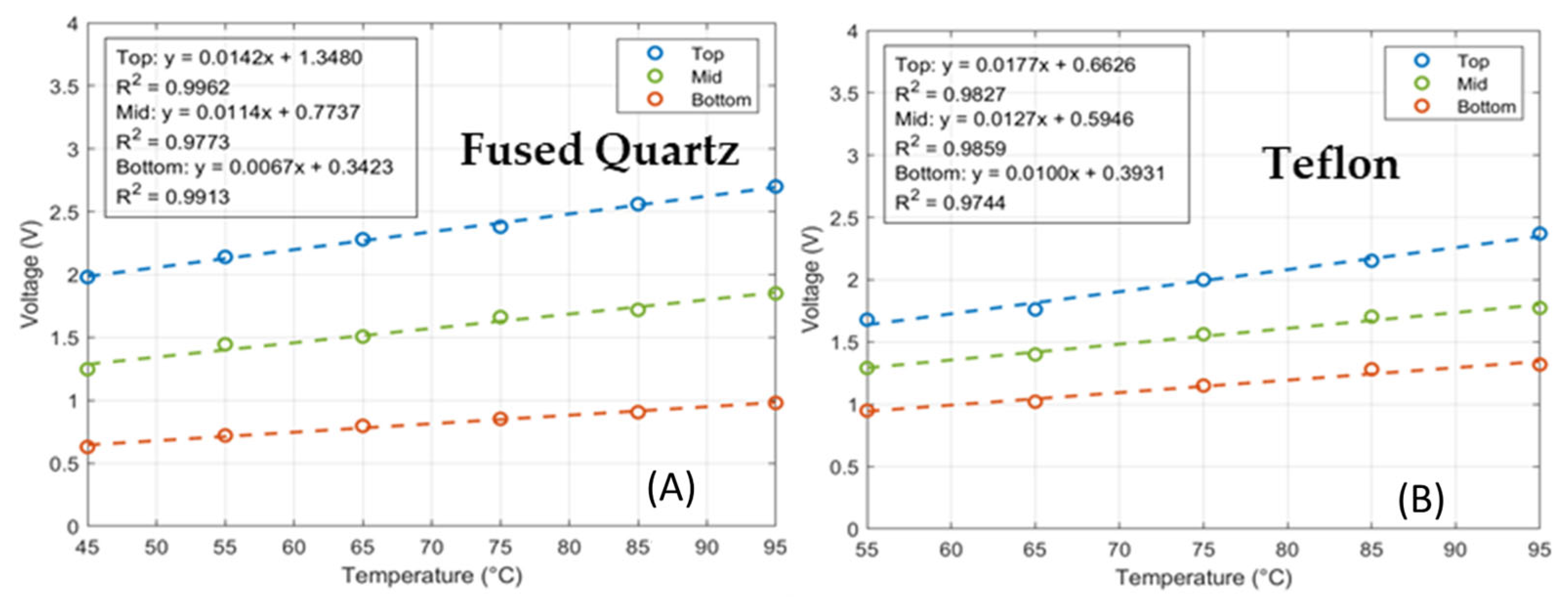
Prior to conducting sample measurements, the apparatus was systematically calibrated using reference materials of known thermal conductivity, fused silica and Teflon, to evaluate stress- and temperature-sensitivity. The sample–meter-disc interfaces were subjected to a controlled axial preload of approximately 200 psi isostatic stress to establish consistent and reproducible initial thermal contact resistance. Figure 3 illustrates the relationship between the top temperature and heater voltage (control power) for the top and bottom guard heaters during guard heater calibration; fused quartz is shown Figure 3A and Teflon in Figure 3B. Both materials exhibit a linear increase in voltage with temperature, confirming predictable, stable PID control behavior. The slopes (~0.017–0.020 V/°C) indicate that fused quartz requires slightly higher guard power than Teflon to maintain equivalent gradients, consistent with its higher thermal conductivity (~1.4 W/m·K) compared to Teflon ~0.25 W/(m·K). The R2 > 0.97 for all regressions validates the proportional control tuning between heating zones. The minor offset between the top and bottom heater voltages confirms balanced but distinct zone responses, as required for thermal symmetry.
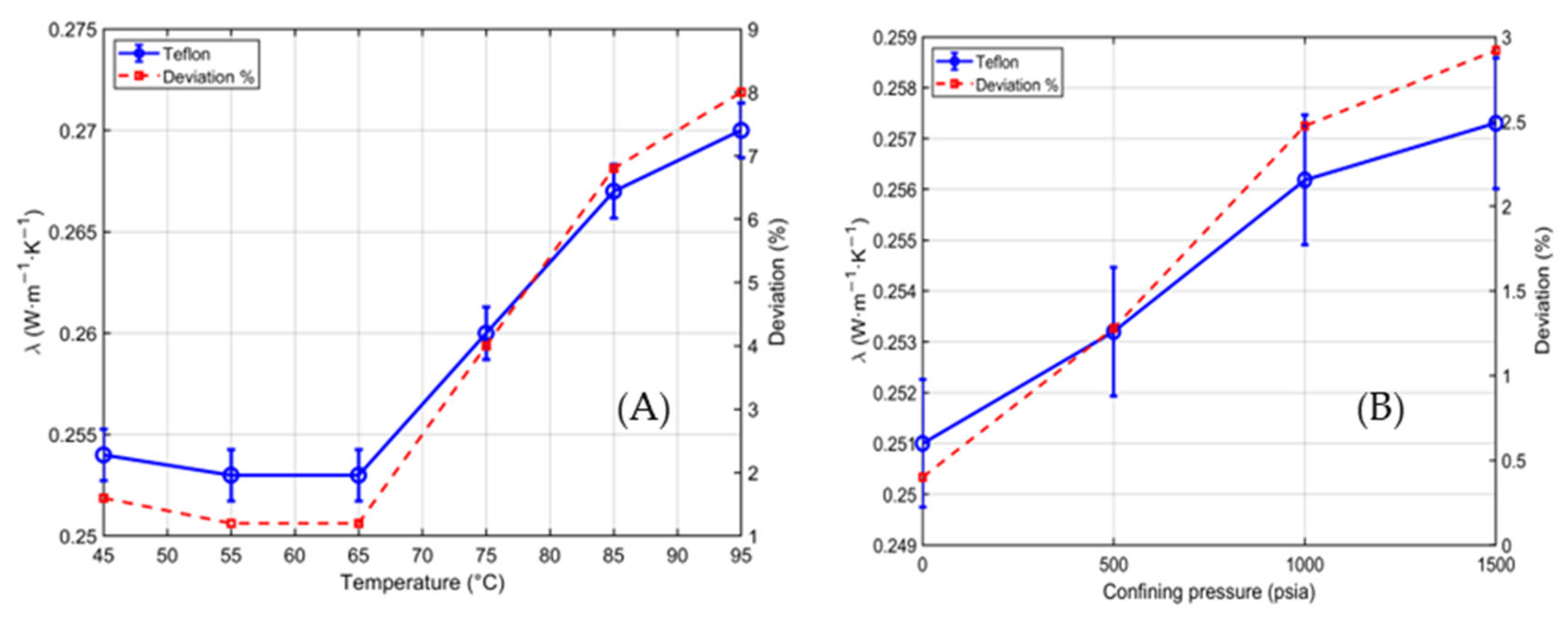
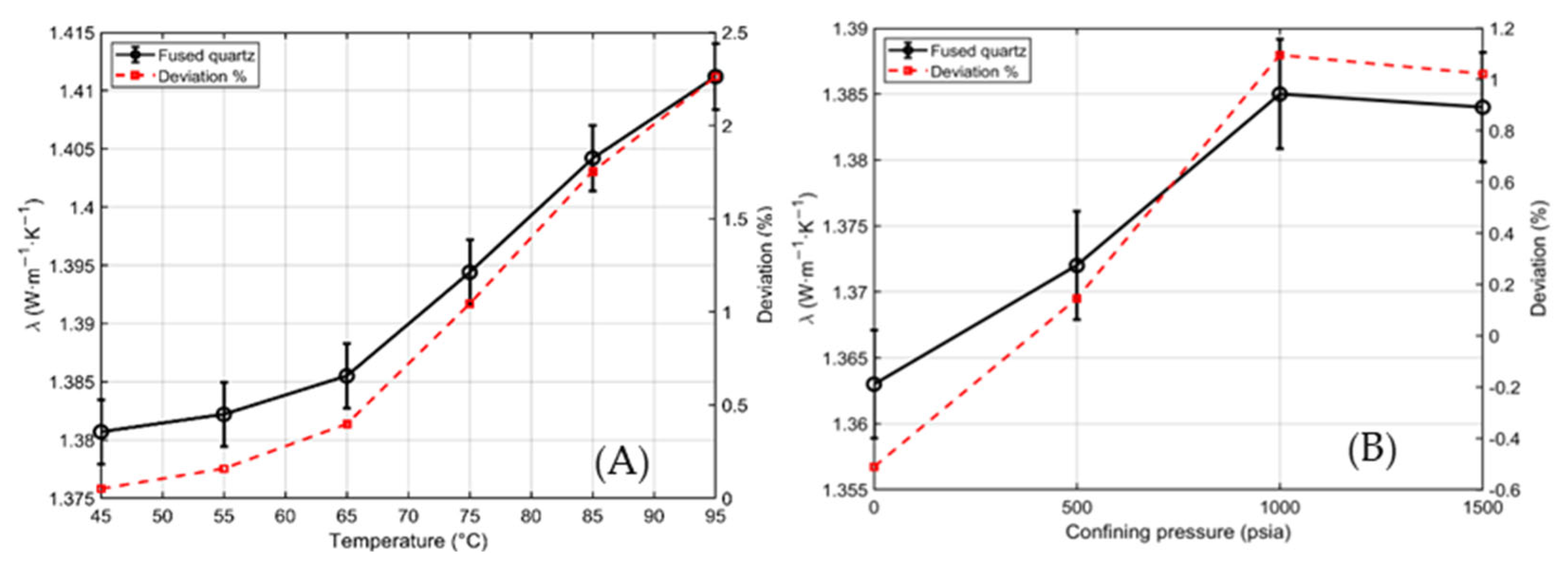
The stress-dependent measurements were performed at controlled confining pressures (0–1500 psi) using argon as the confining gas. During each test, a small differential (deviatoric) axial stress of ~50 psi was applied to ensure mechanical stability and the accuracy of the axial LVDTs. Data acquisition was conducted at multiple pressure increments after confirming steady-state heat flow. Figure 4 shows the small, gradual increase in measured thermal conductivity with temperature, indicating the calibration stability. It also shows a moderate increase in thermal conductivity up to 1500 psi, consistent with reduced interfacial resistance at high pressure. These trends confirm that fused quartz is an excellent calibration reference, owing to its low temperature–pressure sensitivity and reproducible response. Figure 5 shows results for Teflon, indicating a minor increase in thermal conductivity with temperature (from ~0.247 W/m·K to ~0.275 W/m·K), though with slightly larger deviations, reflecting greater sensitivity to temperature fluctuations and a lower thermal diffusivity than quartz. It also shows that Teflon’s measured thermal conductivity increases only slightly with increasing confining pressure, likely due to improved thermal contact between the stack elements. The combined results verify that the divided-bar system maintains a consistent heat-flux balance and predictable thermal performance.

2.2.3. Measurements

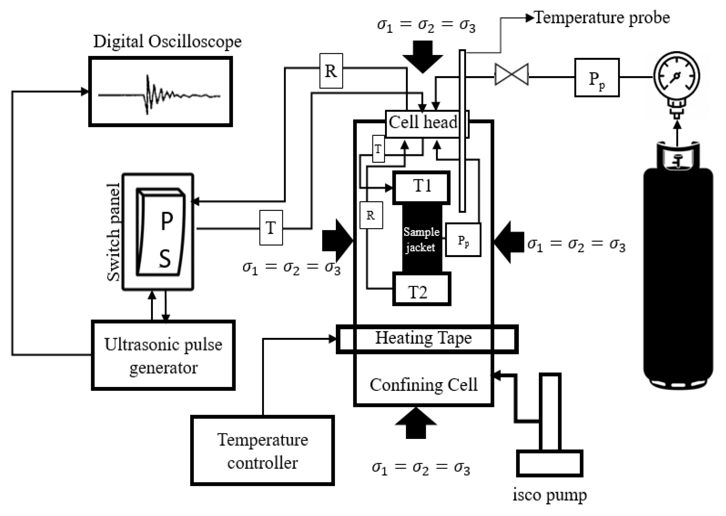
Each sample of Fontainebleau sandstone and the sand packs precisely machined to a length of 1.27 cm and a diameter of 2.5 cm, and then mounted in the divided-bar assembly to obtain stress-dependent thermal conductivity measurements under controlled isostatic loading conditions. Ultrasonic P-wave (compressional) and S-wave (shear) velocities were measured using a stress and temperature-controlled isostatic cell (Figure 6). Each stack was enclosed in a heat-shrink Viton jacket with O-ring seals and a lateral pore-line tap, and positioned between the top and bottom broadband temperature transducers (T1 and T2). The jacketed assembly was secured to the sample holder, with the pore line routed to the cell head for fluid control (Figure 6). The top transducer serves as the source, and the bottom transducer as the receiver, both connected to the external control system via 4-pin Lemo© feedthrough connectors. The confining cell was filled with mineral oil and pressurized using an ISCO© pump to apply constant isostatic stress independent of temperature. The ultrasonic measurements were acquired using the pulse-transmission method, in which a one MHz piezoelectric P/S-wave transducer generates an acoustic pulse that propagates through the sample. The transmitted signal is recorded using a Tektronix TBS-2000 series oscilloscope. Velocities were measured at multiple confining pressures under both dry and water-saturated conditions.

3. Results

3.1. Thermal Conductivity and Acoustic Data for Fontainebleau Sandstone

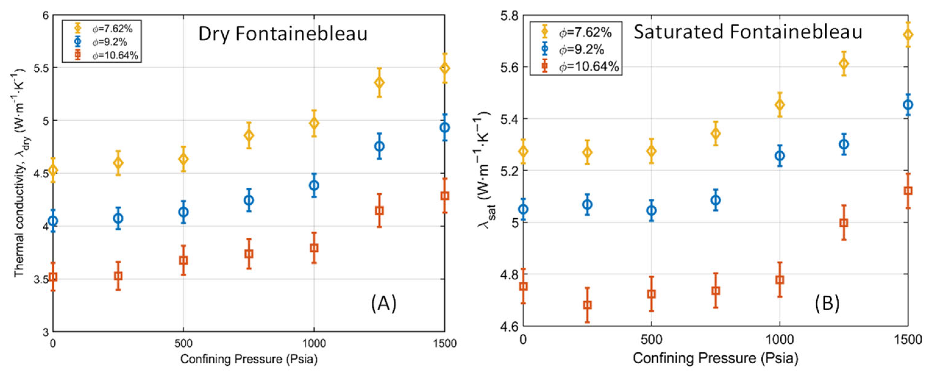
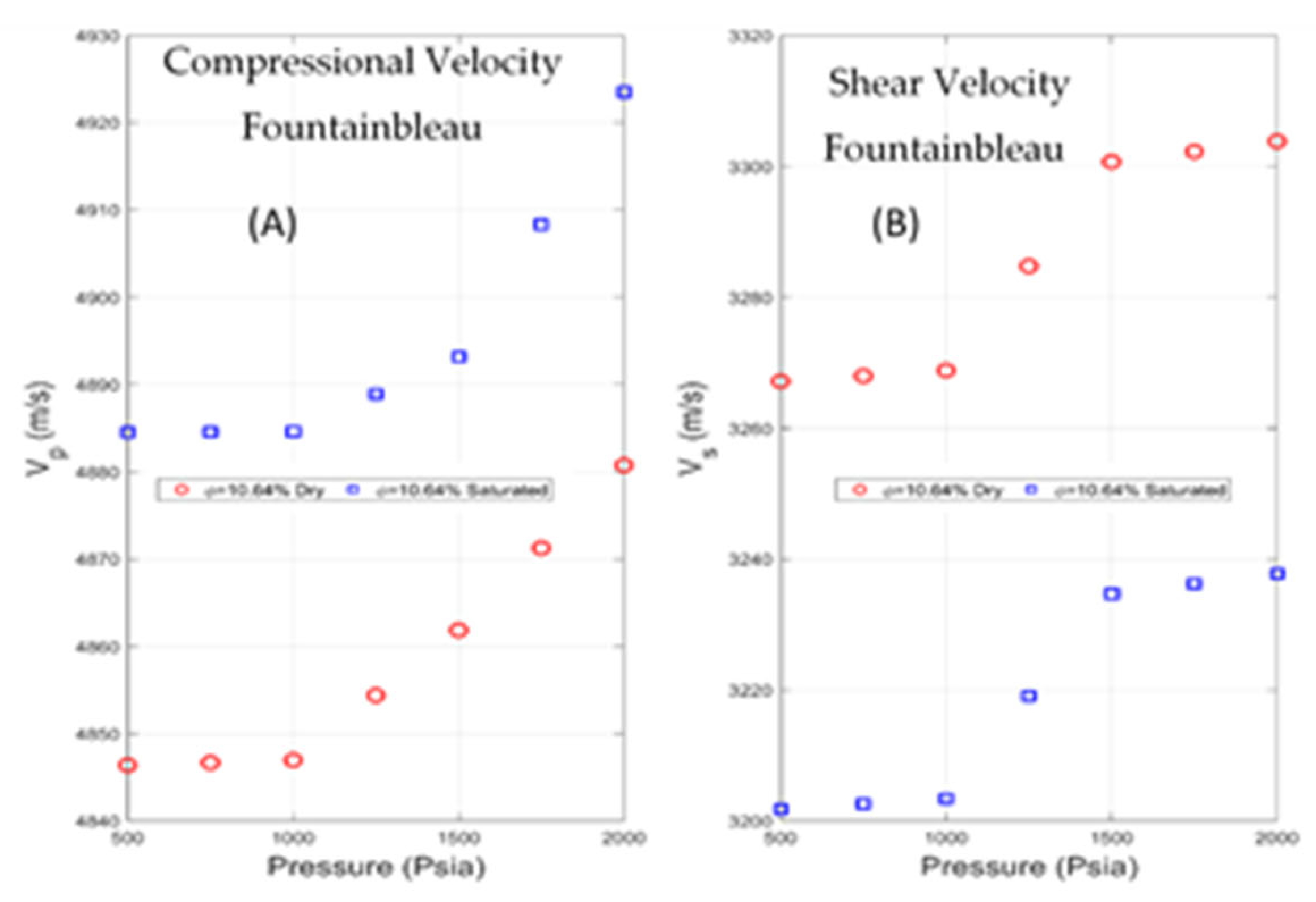
The thermal conductivity of Fontainebleau sandstone increased nonlinearly with confining pressure, and the sample with the lowest porosity exhibited the highest thermal conductivity (Figure 7). Figure 8 shows the measured velocity. The initial lack of stress dependence in both measurements is attributed to the compliance associated with the low initial confining pressure.

3.2. Thermal Conductivity and Acoustic Data for the Sand Packs

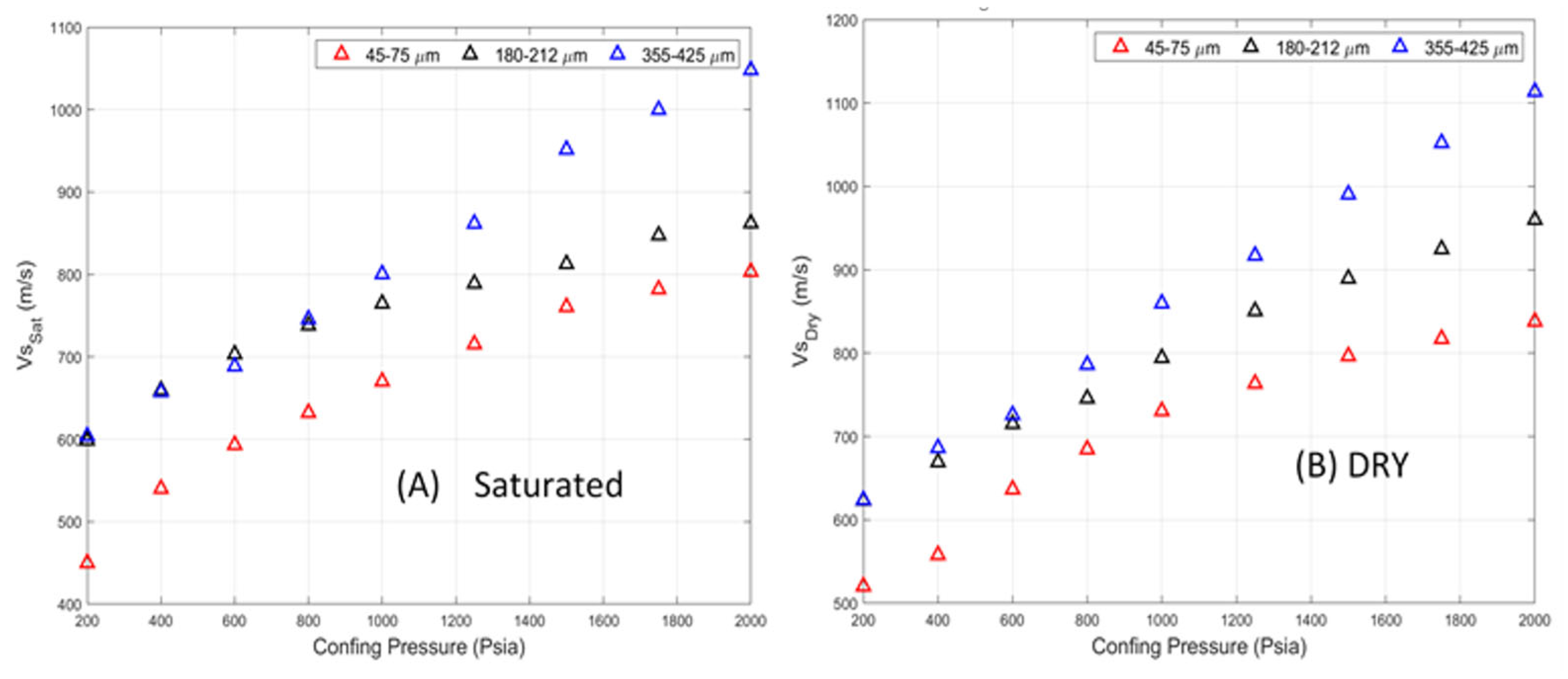
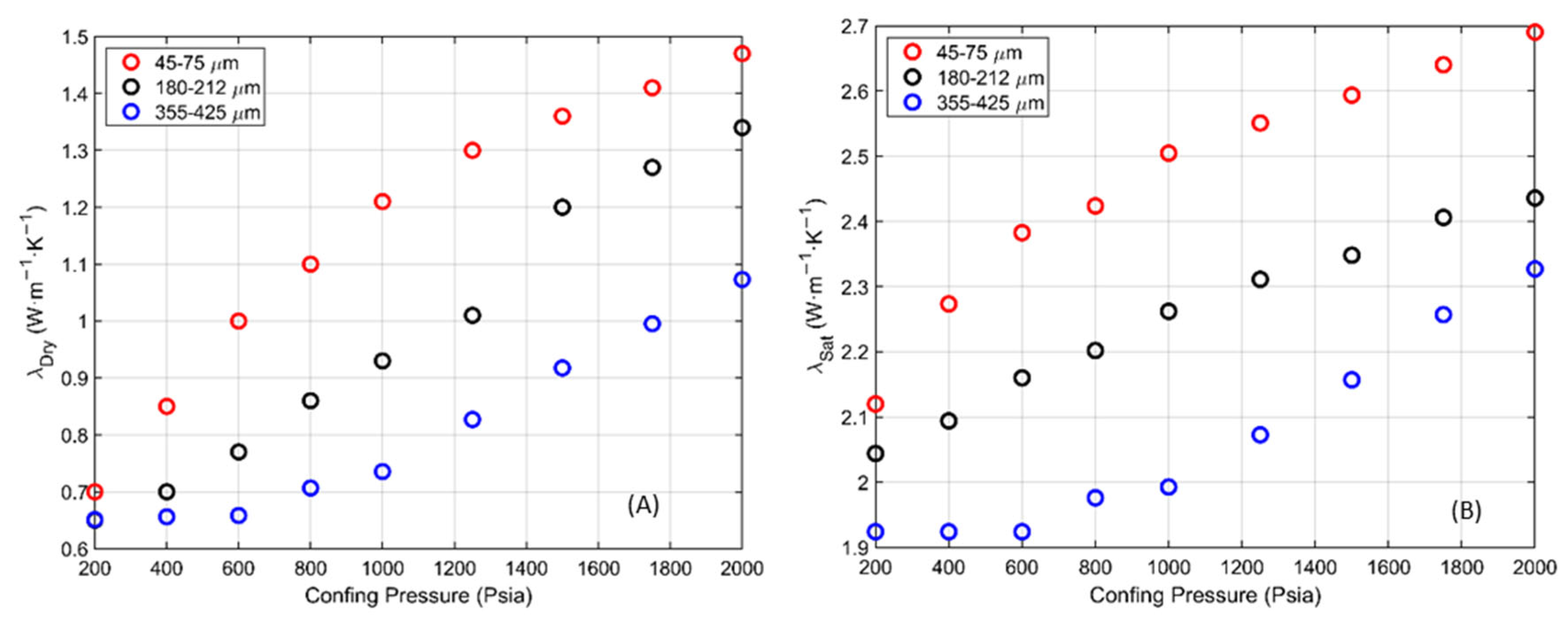
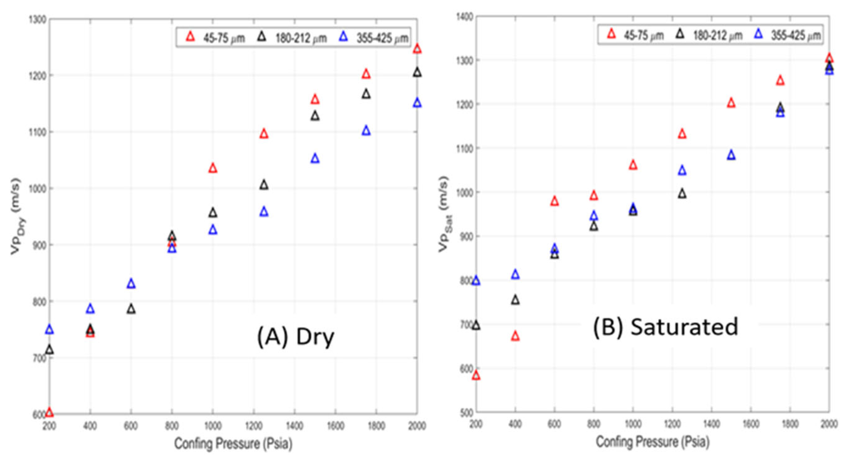
The thermal conductivity cross-plots in Figure 9 demonstrate the similarity of these effects across all samples. In the dry condition (Figure 10A), the thermal conductivity of the sand packs increases with decreasing grain size and confining pressure, after the first two or three stress points where the response is likely dominated by end effects and sample conformance. Water saturation increases the thermal conductivity to nearly twice the dry value (Figure 7A,B). Figure 11A,B show that the compressional wave velocities for the sand packs increase with both confining pressure and saturation, but decrease with grain size. In Figure 12, the shear velocity shows a similar stress dependence but almost no dependence on saturation, and increasing grain size increases the velocity. However, the compressional velocity decreased with increasing grain size. Under saturated conditions, P-wave velocities increase, elevating velocities across all grain sizes compared to the dry state.
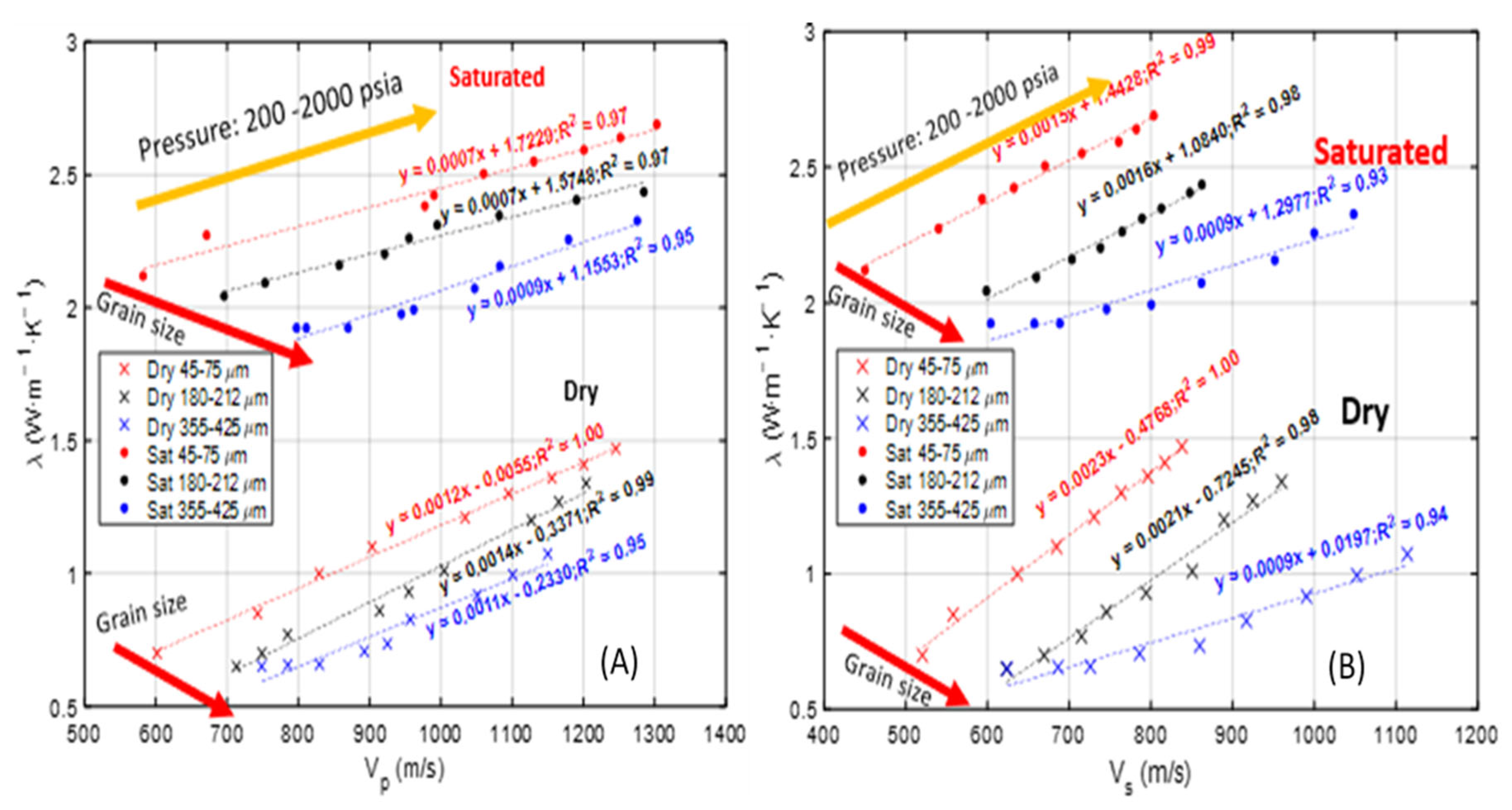
The thermal conductivity and acoustic velocity cross-plot (Figure 12) for the sand packs reveals a strong grain-size dependence. This dependence reflects a balance between grain contact length (favoring fine grains for thermal conductivity and Vp) and grain contact stiffness (favoring coarse grains for Vs). The extremely high correlation coefficients demonstrate the close connection between these effects. Both the modulus and the thermal conductivity are related to the contact percent among framework grains, which increases as a function of decreasing grain size. As grain size decreases in the Brazos bank sand, measured grain aspect ratios increase, resulting in a corresponding increase in grain contact area. The relationship between increasing velocity and contact percentage has been reported previously [50].

4. Discussion

4.1. Formulation of the Staged Differential Effective Medium (SDEM) Model

The Staged Differential Effective Medium (SDEM) framework was introduced for conductive inclusions and later extended [49,50] to model elastic moduli. The method introduces an interpolation parameter. L , where L = 0 corresponds to the Reuss bound and L = 1 describes the Voight bound. The staged approximation allows the model to track rock properties starting from a critical porosity to the zero-porosity endpoint [55]. Porosity is modified in sequential integration steps. The first stage uses L = 0 (suspension) up to the critical porosity, after which a value of L > 0 is applied to reflect the properties of the framework grains as they become load-bearing. This SDEM model incorporates critical porosity behavior and maintains consistency with Gassmann fluid substitution. L corresponds to measurable microstructural attributes, such as contact length and grain-fabric evolution [50]. This staged formulation allows the predicted properties to evolve with changing porosity, rather than imposing a single mixing relation across the full porosity range [51]. Starting from a percolating phase, the ordering of the integration steps is determined by the length scales present in the model. The ordering goes from small to large length scales. Thermal conductivity, like bulk modulus, depends on grain-to-grain contact geometry and is similarly bounded by the Reuss (series or iso-heat flux) and Voigt (parallel or iso-temperature gradient) limits. Substituting thermal conductivity for the bulk modulus in the SDEM model is justified because both are derived from mixture theory. Given this assumption, as shown in Equation (6), the thermal conductivity, λ , is then given by simply substituting the thermal conductivity for the modulus in earlier work [50]:
λ = λ h 1 + ϕ 0 ϕ ϕ 0 · λ i λ h λ h · L 1 ϕ 0 ϕ ϕ 0 · λ i λ h λ i · 1 L
where ϕ 0 is the initial porosity, ϕ is the current porosity, λ i is the thermal conductivity of the inclusion (W/m·K), λ h is the host thermal conductivity (W/m·K), and L is the microstructural fitting parameter. The two-stage model for the effective saturated thermal conductivity ( λ s a t ) In the Reuss average form is:
λ s a t λ i λ s a t = λ d r y λ i λ d r y + ϕ c ϕ · λ L λ i λ L
λ L = ϕ c λ c + 1 ϕ c λ i 1
Equations (7) and (8) are particularly convenient forms for calculating the influence of varying the thermal conductivity of the saturating phase.

4.2. Modeling Fontainebleau Sandstone

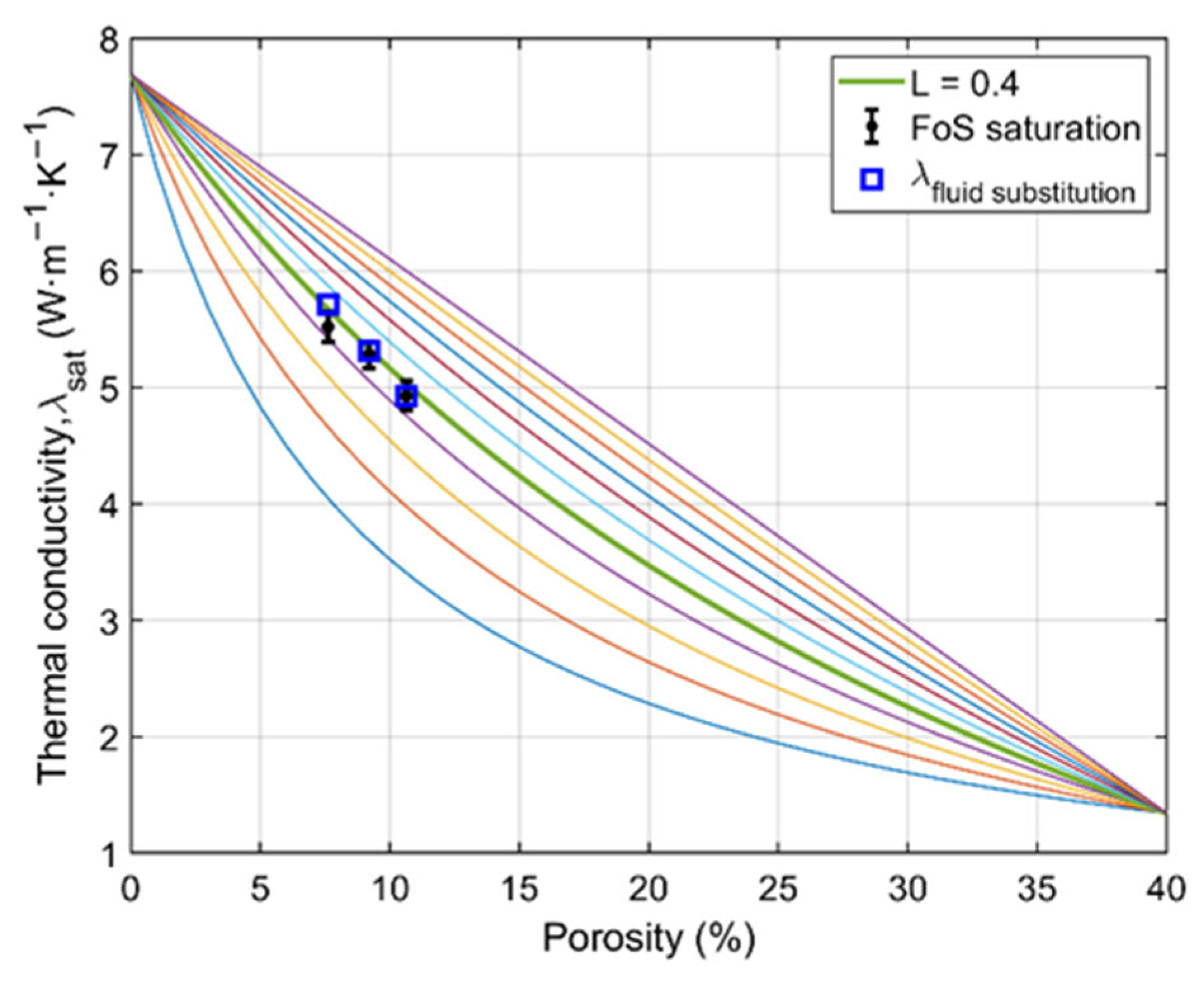
This SDEM model also enables the calculation of thermal conductivity of saturated samples ( λ s a t ) from dry thermal conductivity measurements, analogous to Gassmann’s fluid substitution. Figure 13 shows the thermal conductivity data measured for dry and saturated samples at 1250 psi. The SDEM model uses a quartz matrix thermal conductivity of 7.69 W/m·K for the host phase ( λ h ), and a critical porosity of 40%. For both the dry and saturated thermal conductivity data, the best fit to a single L value is 0.32.
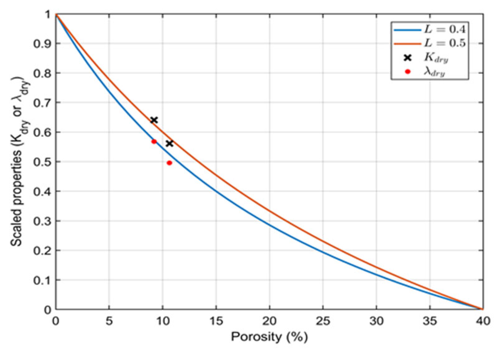
As shown in Figure 14, plotting the thermal conductivity and the bulk modulus on a normalized plot allows a direct comparison between the two measurements. The thermal and elastic properties exhibit similar trends governed by a similar model parameter. The data for the two measurements cluster between the SDEM model curves for L = 0.3 to 0.5, demonstrating that both heat flow and elastic deformation respond to similar but not identical physical properties. The contact modulus dominates the velocity, while thermal conductivity is related to contact thermal resistance. This cross-property calibration capability demonstrates that the model can be used to jointly interpret both types of measurements. This underscores the SDEM model’s value as a unified framework without assuming specific pore geometries such as ellipsoids or cracks, as assumed in prior effective medium theories [39,44].

4.3. SDEM Modeling of Sand Packs

To examine the impact of porosity changes, the largest grain size sand packs were compressed isostatically. As shown in Table 2, the sand packs were compressed isostatically in steps of 3500 psi up to 10,500 psi.
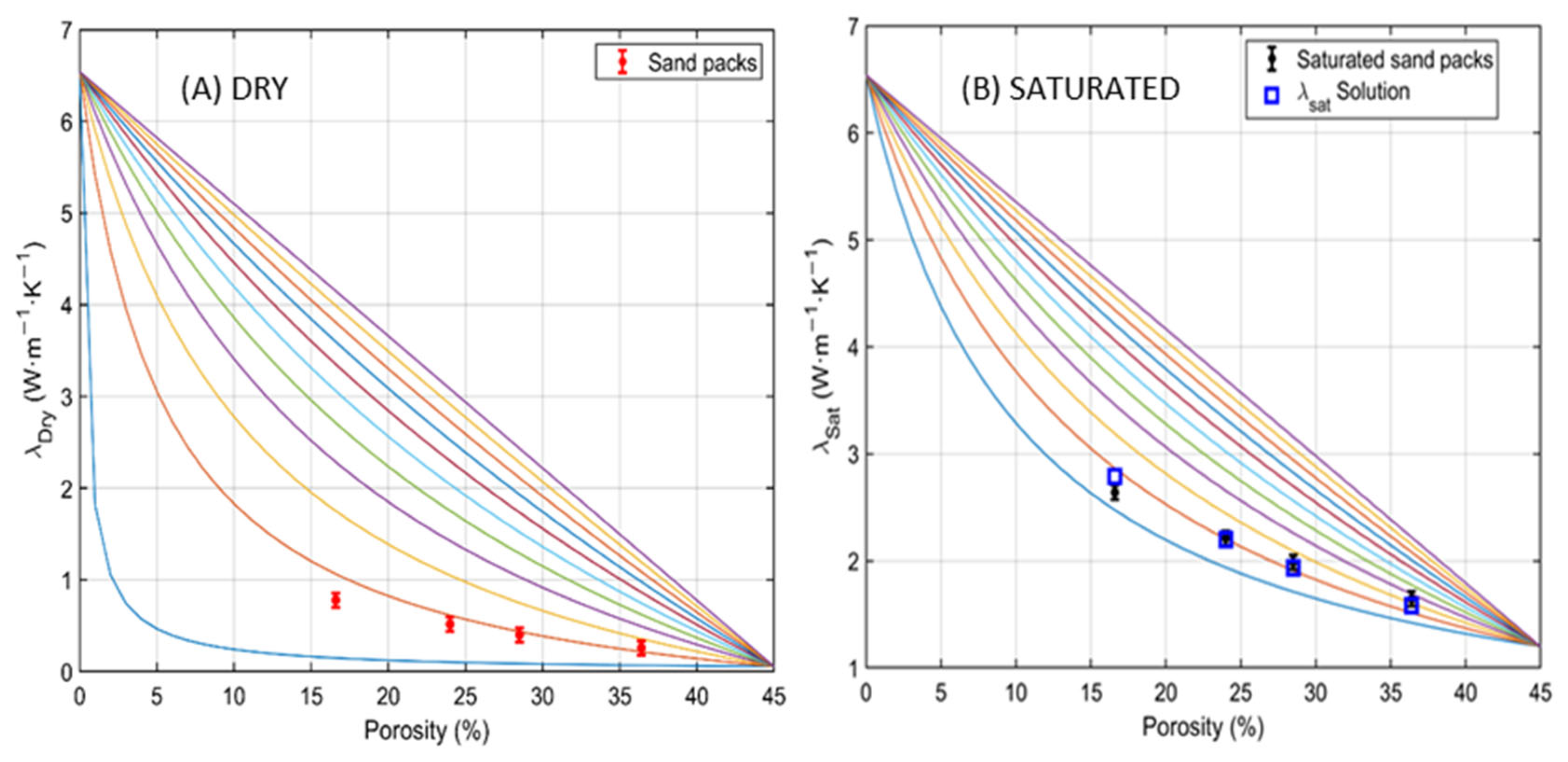
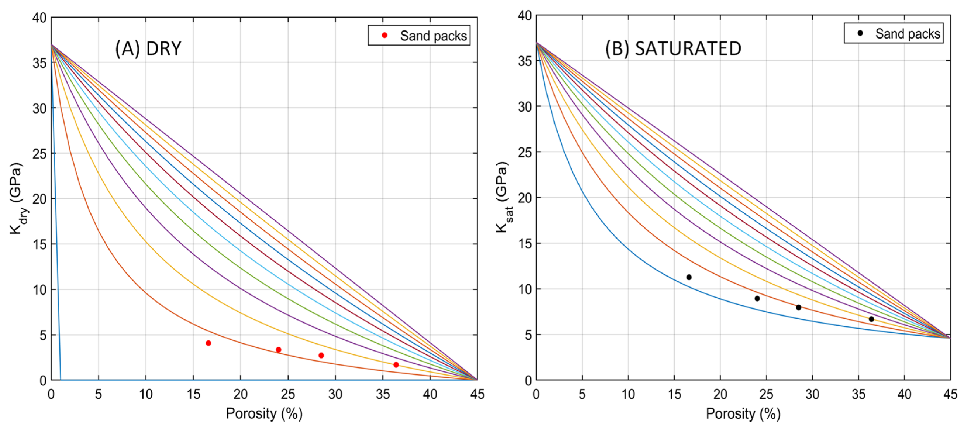
The SDEM modeling results demonstrate that the compaction of the coarse quartz sand (355–425 µm) increases both thermal conductivity (λ) and bulk modulus (K). A single parameter, L~0.12, consistently fits λ and K for both the dry and saturated sand-pack samples (Figure 15 and Figure 16). As porosity decreases, λ and K increase along a constant L value. At the highest compaction level, the model shows a modest change in the associated L value, a discrepancy likely arising from the significant grain crushing that occurs at this high stress. The measured λ s a t values for the coarse sand closely match the SDEM model predictions, confirming that saturation effects are well described by fluid substitution rather than requiring a change in the geometric parameter L. These results show that the SDEM framework tracks the evolution of both the thermal conductivity and the bulk modulus during compaction. This offers a unified tool for interpreting both thermal and elastic responses.

Comparison of Thermal Conductivity Models

In this section, the following models are compared to the SDEM model. All models are expected to fit the thermal conductivity data across the entire porosity range, up to at least the critical porosity.
Wiener bounds [23]:
λ W U = ϕ i λ i + ϕ h λ h
λ H S m e a n = 1 2   ( λ H S L + λ H S U )
λ W L = ϕ i λ i + ϕ h λ h 1
Hashin–Shtrikman upper and lower bounds [33]:
λ H S L = λ f + 3 λ f λ s λ f 1 ϕ 3 λ f + λ s λ f ϕ          
λ H S m e a n = 1 2   ( λ H S L + λ H S U )
λ H S U = λ s + 3 λ s λ f λ s ϕ 3 λ s + λ f λ s 1 ϕ
Maxwell–Eucken [4]:
λ = λ h λ i + 2 λ h + 2 ϕ i λ i λ h λ i + 2 λ h ϕ i λ i λ h
Self-consistent/Bruggeman (EMT) [37,43]:
0 = ϕ h λ h λ λ h + λ + ϕ i λ i λ λ i + 2 λ
Geometric mean [40]:
λ = λ i ϕ i λ h ϕ h
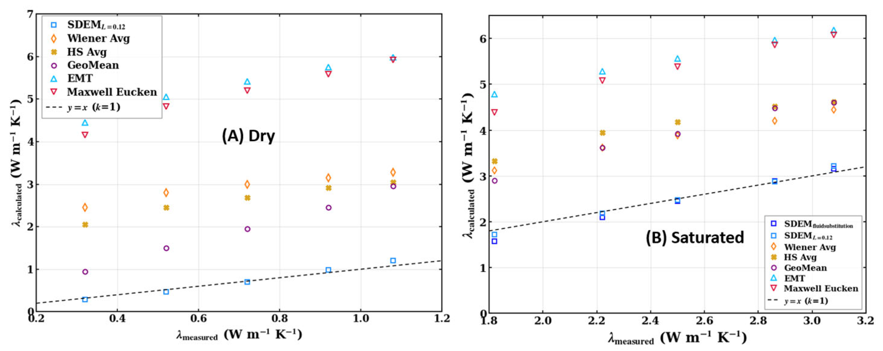
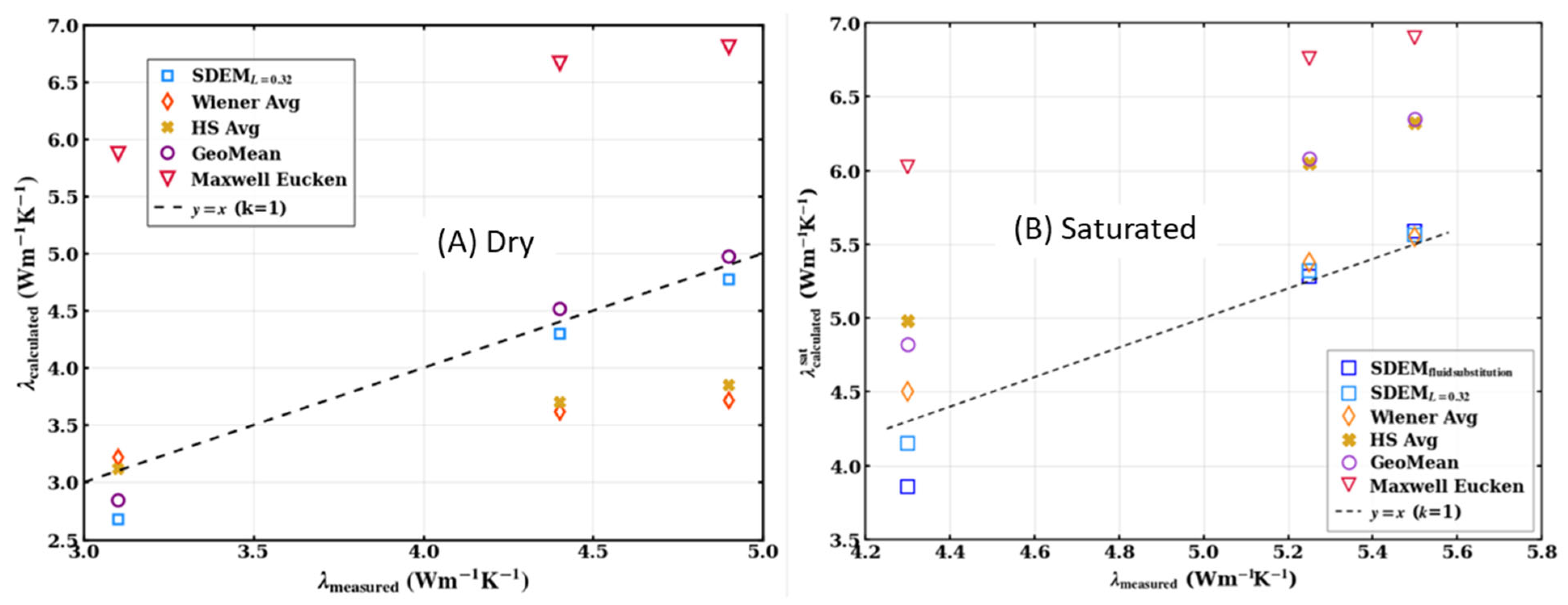
λi is the inclusion thermal conductivity, λh is the host thermal conductivity, and ϕi and ϕh are the porosity of the inclusion and host respectively. Figure 17 illustrates how the different models (SDEM, Wiener Average, HS Average, Geometric Mean, and Maxwell–Eucken models) compare with the measured dry and saturated thermal conductivity.
As shown in Figure 18, the geometric-mean curve matches the Fontainebleau experimental data for both the dry and saturated cases. For the saturated case, the models make predictions similar to those in the dry case. All measurements again lie within the upper and lower bounds, but the test models consistently overestimated λ   s a t . The SDEM with an L = 0.32 yields predictions that again cluster closely around the measured data at all porosities.
Figure 17 shows the comparison between the models and the measured dry and saturated thermal conductivity for the sand packs. All the alternative models predict a thermal conductivity that is too high. The geometric-mean model overpredicts the saturated value. In contrast, SDEM with L = 0.12 yields a prediction that closely matches the data, including the saturation dependence.
The matrix properties determine the different L values for the sand packs and Fontainebleau and correspond to differences in the packing and distribution of thermal pathways within the material. The lower value for the sand packs is closer to a suspension (a lower Wiener bound), which is expected. Fontainebleau, with its higher L value, is closer to the upper bound, consistent with its higher level of cementation.

5. Conclusions

This paper introduces a high-pressure divided-bar apparatus, designed to measure thermal conductivity under controlled confining stresses up to 2000 psi while simultaneously acquiring ultrasonic P- and S-wave velocities. This dual-measurement capability provides insight into the coupled evolution of thermal and elastic properties during compaction.
New experimental datasets on Fontainebleau sandstone and Brazos sandpacks reveal how compaction-driven increases in grain coordination and contact area enhance both thermal conductivity and bulk modulus. These results constitute one of the first systematic demonstrations of how grain size and porosity jointly affect thermal conductivity and velocity. Correlating thermal conductivity with the acoustic velocities measured at identical stress conditions both properties reflect a similar evolving rock frame. This insight enables the use of sonic-log data to infer thermal conductivity profiles, once the relationship is established.
An important contribution is the development and validation of a Staged Differential Effective Medium (SDEM) model that accurately predicts effective thermal conductivity. Across two diverse lithologies, the SDEM model reproduces observed thermal conductivity trends with a single parameter, L, that remains valid under both dry and saturated conditions. This enables a Gassmann-style fluid-substitution capability for thermal conductivity, establishing the SDEM as a powerful and generalizable tool for thermal-conductivity modeling. This modeling also allows the application of the concept of critical concentration to the analysis of thermal conductivity. The classical mixing laws all show systematic biases and fail to capture these fabric effects.
In summary, this work contributes:
  • An advanced experimental platform for high-accuracy thermal measurements.
  • Develops close links between thermal and elastic transport through the application of an SDEM model
  • Introduces the concept of critical concentration models to the prediction of thermal conductivity.
These findings strengthen the theoretical foundation of rock thermal transport, improve prediction accuracy beyond classical approaches, and open new pathways for integrating thermal, electrical, and acoustic observations in subsurface characterization.
Future work will include the impact of changes in mineralogy. As the framework mineralogy changes, so do the grain contact % and the thermal conductivity of the starting material. In feldspathic sands, for example, at a low concentration of feldspar, increases in the contact % among grains will impact the measured conductivity more than the small decrease that should result from the mineralogic change. As feldspar increases, contact % will continue to rise, which should increase thermal conductivity, but the starting thermal conductivity of the sand’s solid components will be lower. This complexity will require measuring multiple sand packs with progressively more varied mineralogy and conducting detailed image analysis to document the structural changes in the material. As such, a detailed inclusion of mineralogic changes is beyond the scope of this paper.

Author Contributions

Conceptualization, M.T.M.; methodology, Y.C., M.T.M., G.C.U. and D.M.; Software, Y.C.; formal analysis, Y.C.; investigation, Y.C., M.T.M., L.H., G.C.U. and D.M.; writing—original draft, Y.C.; writing—review and editing, M.T.M., L.H. and G.C.U.; supervision, M.T.M. and Lori Hathon; project administration, M.T.M. All authors have read and agreed to the published version of the manuscript.

Funding

This research received no external funding.

Data Availability Statement

The original contributions presented in this study are included in the article. Further inquiries can be directed to the corresponding author.

Conflicts of Interest

The authors declare no conflicts of interest.

References

  1. Carslaw, H.S.; Jaeger, J.C. Conduction of Heat in Solids, 2nd ed.; Oxford University Press: Oxford, UK, 1959. [Google Scholar]
  2. García-Noval, C.; Álvarez, R.; García-Cortés, S.; García, C.; Alberquilla, F.; Ordóñez, A. Definition of a thermal conductivity map for geothermal purposes. Geotherm. Energy 2024, 12, 17. [Google Scholar] [CrossRef]
  3. Preux, C.; Malinouskaya, I. Thermal conductivity model function of porosity: Review and fitting using experimental data. Oil Gas Sci. Technol. Rev. IFP Energies Nouv. 2021, 76, 66. [Google Scholar] [CrossRef]
  4. Clauser, C.; Huenges, E. Thermal conductivity of rocks and minerals. In Rock Physics & Phase Relations: A Handbook of Physical Constants; Ahrens, T.J., Ed.; American Geophysical Union: Washington, DC, USA, 1995; Volume 3, pp. 105–126. [Google Scholar]
  5. Raymond, J.; Langevin, H.; Comeau, F.-A.; Malo, M. Temperature dependence of rock salt thermal conductivity: Implications for geothermal exploration. Renew. Energy 2022, 184, 26–35. [Google Scholar] [CrossRef]
  6. Mokheimer, E.M.; Hamdy, M.; Abubakar, Z.; Shakeel, M.R.; Habib, M.A.; Mahmoud, M. A comprehensive review of thermal enhanced oil recovery: Techniques evaluation. J. Energy Resour. Technol. 2019, 141, 030801. [Google Scholar] [CrossRef]
  7. Horai, K.-I. Thermal conductivity of rock-forming minerals. J. Geophys. Res. 1971, 76, 1278–1308. [Google Scholar] [CrossRef]
  8. Brigaud, F.; Vasseur, G. Mineralogy, porosity and fluid control on thermal conductivity of sedimentary rocks. Geophys. J. Int. 1989, 98, 525–542. [Google Scholar] [CrossRef]
  9. Hermans, T.; Nguyen, F.; Robert, T.; Revil, A. Geophysical methods for monitoring temperature changes in shallow low enthalpy geothermal systems. Energies 2014, 7, 5083–5118. [Google Scholar] [CrossRef]
  10. Raymond, J. Colloquium 2016: Assessment of subsurface thermal conductivity for geothermal applications. Can. Geotech. J. 2018, 55, 1209–1229. [Google Scholar] [CrossRef]
  11. Beck, A.E.; Jaeger, J.; Newstead, G. The measurements of the thermal conductivities of rocks by observations in boreholes. J. Geophys. Res. 1971, 76, 3391–3401. [Google Scholar] [CrossRef]
  12. Clauser, C.; Huenges, E. Thermal properties of rocks and minerals. In Rock Physics & Phase Relations: A Handbook of Physical Constants; Ahrens, T.J., Ed.; American Geophysical Union: Washington, DC, USA, 1995. [Google Scholar]
  13. Hyndman, R.D.; Langseth, M.G.; von Herzen, R.P. A review of Deep Sea Drilling Project geothermal measurements through Leg 71. Initial Rep. Deep Sea Drill. Proj. 1984, 78, 813–823. [Google Scholar]
  14. Gehlin, S. Thermal Response Test: Method Development and Evaluation. Ph.D. Thesis, Luleå University of Technology, Luleå, Sweden, 2002. [Google Scholar]
  15. Cheng, L.; Zhang, Y.; Zhang, A.; Sun, Y.; Cao, Y.; Xu, Z. Investigation of measurement methods for soil thermal conductivity based on optical frequency domain reflection technology. Int. J. Therm. Sci. 2024, 198, 108889. [Google Scholar] [CrossRef]
  16. Dalla Santa, G.; Peron, F.; Galgaro, A.; Cultrera, M.; Bertermann, D.; Müller, J.; Bernardi, A. An updated ground thermal properties database for ground source heat pump applications. Energy 2020, 193, 116727. [Google Scholar]
  17. Parker, W.J.; Jenkins, R.J.; Butler, C.P.; Abbott, G.L. Flash method of determining thermal diffusivity, heat capacity, and thermal conductivity. J. Appl. Phys. 1961, 32, 1679–1684. [Google Scholar] [CrossRef]
  18. Sass, J.H.; Lachenbruch, A.H.; Munroe, R.J.; Greene, G.W.; Moses, T.H. Heat flow in the western United States. J. Geophys. Res. 1971, 76, 6376–6413. [Google Scholar] [CrossRef]
  19. Jaeger, J.C. The use of complete temperature-time curves for the determination of thermal conductivity, with particular reference to rocks. Aust. J. Phys. 1959, 12, 203–214. [Google Scholar] [CrossRef]
  20. Popov, Y.A.; Pribnow, D.F.C.; Sass, J.H.; Williams, C.F.; Burkhardt, H. Characterization of rock thermal conductivity by high-resolution optical scanning. Geothermics 1999, 28, 253–276. [Google Scholar] [CrossRef]
  21. Hammerschmidt, U.; Meier, V. New transient hot bridge sensor to measure thermal conductivity, thermal diffusivity, and volumetric specific heat. Int. J. Thermophys. 2006, 27, 840–865. [Google Scholar] [CrossRef]
  22. Schön, J.H. Physical Properties of Rocks: A Workbook; Elsevier: Amsterdam, The Netherlands, 2011. [Google Scholar]
  23. Wiener, O. Theorie des Mischkörpers für das Feld der Stationären Strömung; B.G. Teubner: Leipzig, Germany, 1912; pp. 509–598. [Google Scholar]
  24. Fuchs, S.; Förster, A.; Förster, H.-J. Evaluation of common mixing models for calculating bulk thermal conductivity of sedimentary rocks: Correction charts and new conversion equations. Geothermics 2013, 47, 40–52. [Google Scholar] [CrossRef]
  25. Goutorbe, B.; Lucazeau, F.; Bonneville, A. Comparison of several BHT correction methods: A case study on an Australian dataset. Geophys. J. Int. 2006, 164, 104–118. [Google Scholar] [CrossRef]
  26. Hartmann, A.; Rath, V.; Clauser, C. Thermal conductivity from core and well log data. Int. J. Rock Mech. Min. Sci. 2005, 42, 1042–1055. [Google Scholar] [CrossRef]
  27. Waqas, U.; Rashid, H.M.A.; Ahmed, M.F.; Rasool, A.M.; Al-Atroush, M.E. Damage characteristics of thermally deteriorated carbonate rocks: A review. Appl. Sci. 2022, 12, 2752. [Google Scholar] [CrossRef]
  28. Mielke, P.; Bär, K.; Sass, I. Determining the relationship of thermal conductivity and compressional wave velocity of common rock types as a basis for reservoir characterization. J. Appl. Geophys. 2017, 140, 135–144. [Google Scholar] [CrossRef]
  29. Abdulagatova, Z.; Abdulagatov, I.M.; Emirov, V.N. Effect of temperature and pressure on the thermal conductivity of sandstone. Int. J. Rock Mech. Min. Sci. 2009, 46, 1055–1071. [Google Scholar] [CrossRef]
  30. Labus, K.; Labus, M.; Bujok, P.; Wysocka, M. Influence of temperature on thermal conductivity of selected rocks. J. Therm. Anal. Calorim. 2018, 134, 1779–1787. [Google Scholar]
  31. Vosteen, H.-D.; Schellschmidt, R. Influence of temperature on thermal conductivity, thermal capacity and thermal diffusivity for different types of rock. Phys. Chem. Earth 2003, 28, 499–509. [Google Scholar]
  32. Fuchs, S.; Förster, H.-J.; Norden, B.; Balling, N.; Mielke, R.; Heckenbach, E.; Förster, A. The thermal diffusivity of sedimentary rocks: Empirical validation of a physically based α–φ relation. J. Geophys. Res. Solid Earth 2021, 126, e2020JB020595. [Google Scholar] [CrossRef]
  33. Hashin, Z.; Shtrikman, S. A variational approach to the theory of the effective magnetic permeability of multiphase materials. J. Appl. Phys. 1962, 33, 3125–3131. [Google Scholar] [CrossRef]
  34. Maxwell, J.C. A Treatise on Electricity and Magnetism; Clarendon Press: Oxford, UK, 1873. [Google Scholar]
  35. Eucken, A. Allgemeine Gesetzmäßigkeiten für das Wärmeleitvermögen verschiedener Stoffarten und Aggregatzustände. Forsch. Geb. Ingenieurwes. A 1940, 11, 6–20. [Google Scholar] [CrossRef]
  36. Levy, F. A modified Maxwell–Eucken equation for calculating the thermal conductivity of two-component solutions or mixtures. Int. J. Refrig. 1981, 4, 223–225. [Google Scholar] [CrossRef]
  37. Berryman, J.G. Mixture theories for rock properties. In Rock Physics & Phase Relations: A Handbook of Physical Constants; Ahrens, T.J., Ed.; American Geophysical Union: Washington, DC, USA, 1995; pp. 205–228. [Google Scholar]
  38. Norris, A.N. A differential scheme for the effective moduli of composites. Mech. Mater. 1985, 4, 1–16. [Google Scholar] [CrossRef]
  39. Mavko, G.; Mukerji, T.; Dvorkin, J. The Rock Physics Handbook, 3rd ed.; Cambridge University Press: Cambridge, UK, 2020. [Google Scholar]
  40. Woodside, W.; Messmer, J.H. Thermal conductivity of porous media. I. Unconsolidated sands. J. Appl. Phys. 1961, 32, 1688–1699. [Google Scholar] [CrossRef]
  41. Fuchs, S.; Förster, H.-J.; Braune, K.; Förster, A. Calculation of thermal conductivity of low-porous, isotropic plutonic rocks of the crust at ambient conditions from modal mineralogy and porosity: A viable alternative for direct measurement? J. Geophys. Res. Solid Earth 2018, 123, 8602–8614. [Google Scholar] [CrossRef]
  42. Ghanbarian, B.; Daigle, H. Thermal conductivity in porous media: Percolation-based effective-medium approximation. Water Resour. Res. 2016, 52, 295–314. [Google Scholar] [CrossRef]
  43. Zimmerman, R.W. Thermal conductivity of fluid-saturated rocks. J. Pet. Sci. Eng. 1989, 3, 219–227. [Google Scholar] [CrossRef]
  44. Pimienta, L.; Sarout, J.; Esteban, L.; Delle Piane, C. Prediction of rocks thermal conductivity from elastic wave velocities, mineralogy and microstructure. Geophys. J. Int. 2014, 197, 860–874. [Google Scholar] [CrossRef]
  45. El Sayed, A.M.A.; El Sayed, N.A. Thermal conductivity calculation from P-wave velocity and porosity assessment for sandstone reservoir rocks. Geothermics 2019, 82, 91–96. [Google Scholar] [CrossRef]
  46. Gegenhuber, N.; Schön, J. New approaches for the relationship between compressional wave velocity and thermal conductivity. J. Appl. Geophys. 2012, 76, 50–55. [Google Scholar] [CrossRef]
  47. Orlander, T.; Adamopoulou, E.; Jerver Asmussen, J.; Marczyński, A.A.; Milsch, H.; Pasquinelli, L.; Lykke Fabricius, I. Thermal conductivity of sandstones from Biot’s coefficient. Geophysics 2018, 83, D173–D185. [Google Scholar] [CrossRef]
  48. Esteban, L.; Pimienta, L.; Sarout, J.; Delle Piane, C.; Haffen, S.; Géraud, Y.; Timms, N.E. Study cases of thermal conductivity prediction from P-wave velocity and porosity. Geothermics 2015, 53, 255–269. [Google Scholar] [CrossRef]
  49. Myers, M. Pore modeling: Extending the Hanai–Bruggeman equation. In Proceedings of the SPWLA 30th Annual Logging Symposium, Houston, TX, USA, 11–14 June 1989. [Google Scholar]
  50. Myers, M.; Hathon, L. Staged differential effective medium (SDEM) models for acoustic velocity. In SEG Technical Program Expanded Abstracts 2009; Society of Exploration Geophysicists: Tulsa, OK, USA, 2009; pp. 2130–2134. [Google Scholar]
  51. Villarroel, A.; Myers, M.; Hathon, L. Integrating Thomas–Stieber with a staged differential effective medium model for saturation interpretation of thin-bedded shaly sands. In Proceedings of the SPWLA 63rd Annual Logging Symposium, Stavanger, Norway, 25–29 June 2022. [Google Scholar]
  52. Myers, M.; Hathon, L. Staged differential effective medium (SDEM) models for the acoustic velocity in carbonates. In Proceedings of the ARMA US Rock Mechanics/Geomechanics Symposium, Chicago, IL, USA, 24–27 June 2012; American Rock Mechanics Association: Alexandria, VA, USA, 2012. [Google Scholar]
  53. Thiry, M.; Bertrand-Ayrault, M.; Grisoni, J.-C. Groundwater silicification and leaching in sands: Example of the Fontainebleau Sand (Oligocene) in the Paris Basin. Geol. Soc. Am. Bull. 1988, 100, 1283–1290. [Google Scholar] [CrossRef]
  54. ASTM E1225-13; Standard Test Method for Thermal Conductivity of Solids Using the Guarded Comparative-Longitudinal Heat Flow Technique. ASTM International: West Conshohocken, PA, USA, 2013.
  55. Nur, A.; Mavko, G.; Dvorkin, J.; Galmudi, D. Critical porosity: A key to relating physical properties to porosity in rocks. Lead. Edge 1998, 17, 357–362. [Google Scholar] [CrossRef]
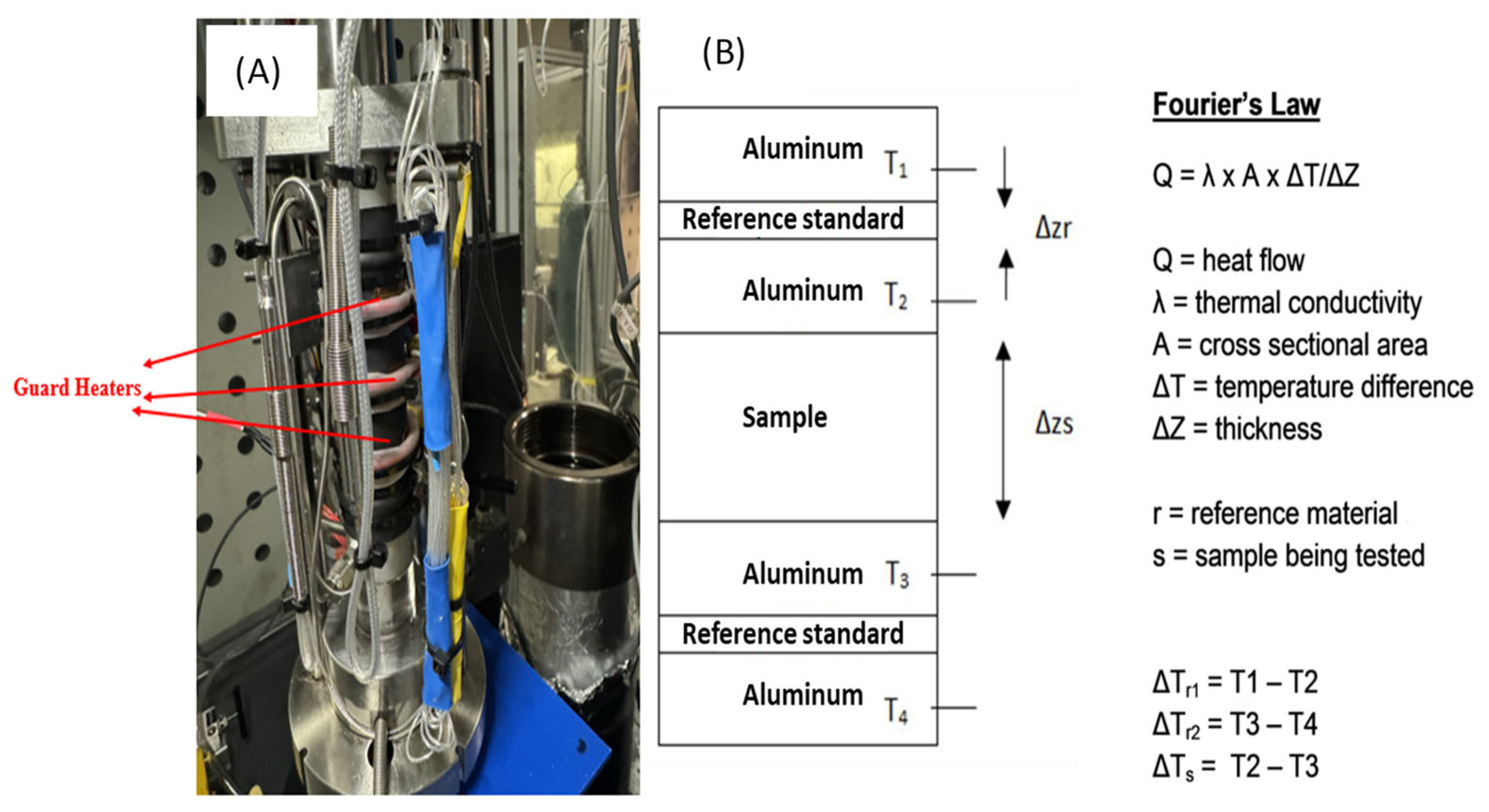
Figure 1. Viton sleeved high-pressure thermal conductivity measurement stack with embedded reference discs, thermocouples, and heater wiring (A). Sketch of the experimental sample and reference stack (B).
Processes 14 01437 g001
Figure 2. Temperature control performance illustrating the PID regulation (A). Zoomed view of a representative time interval of the equilibrated measurement, T1 showing the high thermal stability (B). The gradient evolution for top and bottom reference zones during PID control (C).
Processes 14 01437 g002
Figure 3. Calibration measurements confirming heater voltages for two standards. Guard heater voltage versus top temperature (3-Zone Control) for fused quartz (A) and Teflon (B).
Processes 14 01437 g003
Figure 4. Fused quartz measurement with respect to temperature (A) and confining pressure (B). The small variation in thermal conductivity with temperature and pressure validates the equipment stability.
Processes 14 01437 g004
Figure 5. Results of the measurement of Teflon with respect to temperature (A) and confining pressure (B). The higher thermal conductivity is consistent with the higher voltages required in Figure 3.
Processes 14 01437 g005
Figure 6. Diagram of the stress–temperature-dependent acoustic measurements system. This represents the first time that a stress-dependent measurement system has been constructed. The arrows indicate the direction of the stress.
Processes 14 01437 g006
Figure 7. (A) Measurements of dry thermal conductivity for Fontainebleau sandstone. (B) Brine saturated thermal conductivity. The lack of stress dependence at low stress is interpreted as compliance effects in the samples and equipment.
Processes 14 01437 g007
Figure 8. (A) is the confining pressure dependence of the compressional wave velocity (Vp). (B) is the shear wave velocity (Vs) for the Fontainebleau sandstone (10.6% porosity). The velocity is measured under dry (red circles) and water-saturated (blue squares) conditions.
Processes 14 01437 g008
Figure 9. (A) is the measured thermal conductivity of saturated and dry sand packs for different grain sizes as a function of confining pressure. (B) shows that the larger grain sizes have lower thermal conductivities. The thermal conductivity also increased with stress.
Processes 14 01437 g009
Figure 10. Measured compressional velocities of dry (A) and saturated sand packs (B) of different grain sizes as a function of confining pressure. Smaller grain sizes have higher compressional velocities.
Processes 14 01437 g010
Figure 11. Measured shear velocities of saturated (A) and dry (B) sand packs of different grain sizes as a function of confining pressure. Larger grain sizes have higher shear velocities.
Processes 14 01437 g011
Figure 12. Stress-dependent linear regression of thermal conductivity with Vp (A) and Vs (B) for different grain size sand packs. There are excellent correlations between velocity and thermal conductivity, reflecting common trends between contact moduli (velocities) and contact resistance (thermal conductivity).
Processes 14 01437 g012
Figure 13. Measured thermal conductivity of dry and saturated Fontainebleau sandstones plotted against porosity, along with SDEM model predictions for different L values. Solid colored curves represent SDEM models for various geometric parameters L. The critical porosity, ϕc = 40%. The squares are the predicted saturated values calculated by fluid substitution from the dry measurements. The best fit for all the measurements gives L = 0.32.
Processes 14 01437 g013
Figure 14. Normalized properties for dry thermal conductivity (λ) and bulk modulus (K) in the SDEM model for Fountainbleu sandstone.
Processes 14 01437 g014
Figure 15. The SDEM model curves for compaction of coarse quartz sand for dry (A) and saturated conditions. (B) is both the fluid substitution model (square symbols) and the data. The critical porosity is assumed to be 45% for the sandpacks.
Processes 14 01437 g015
Figure 16. The SDEM model curves for the bulk modulus as a function of compaction of coarse quartz sand under dry (A) and saturated conditions. (B) is the saturated data. The critical porosity is assumed to be 45%. The best fit for sand packs is L= 0.12, significantly lower than the value found for Fontainebleau sandstone.
Processes 14 01437 g016
Figure 17. Comparison between measured and calculated dry (A) and water-saturated (B) thermal conductivity of the sand pack samples. The SDEM model uses a single fitted parameter of 0.12, which fits both the dry and saturated samples. All of the other models overpredict the data.
Processes 14 01437 g017
Figure 18. Comparison between measured and calculated dry (A) and water-saturated (B) thermal conductivity of the Fontainebleau sandstone samples. The SDEM model uses a single fitted parameter, 0.32, across all data.
Processes 14 01437 g018
Table 1. Grain Size-Dependent Sand Pack Properties.
SampleMineralogyPorosity (%)Grain Size (μm)
1Brazos River36.9745–75
2Sand over 95%37.10180–212
3quartz36.23355–425
Table 2. Resultant change in axial strain and porosity at the end of each isostatic compaction stage.
StagePorosity (%)Axial Strain (%)Stress (psi)
137.000
228.612.43500
324.019.57000
416.731.210,500
Disclaimer/Publisher’s Note: The statements, opinions and data contained in all publications are solely those of the individual author(s) and contributor(s) and not of MDPI and/or the editor(s). MDPI and/or the editor(s) disclaim responsibility for any injury to people or property resulting from any ideas, methods, instructions or products referred to in the content.