Article

Super-Resolution Enhancement of Fiber-Optic LF-DAS for Closely Spaced Fracture Monitoring During Hydraulic Fracturing

1
State Key Laboratory of Petroleum Resources and Engineering, China University of Petroleum (Beijing), Beijing 102249, China
2
Key Laboratory of Petroleum Engineering, China University of Petroleum (Beijing), Beijing 102249, China
3
CNPC Engineering Technology R&D Company Limited, Beijing 102206, China
*
Author to whom correspondence should be addressed.
Processes 2026, 14(9), 1380; https://doi.org/10.3390/pr14091380
Submission received: 20 March 2026 / Revised: 14 April 2026 / Accepted: 22 April 2026 / Published: 25 April 2026

Abstract

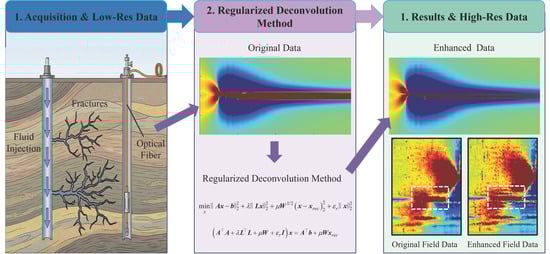
Hydraulic fracturing of unconventional reservoirs requires accurate fracture monitoring for treatment optimization. Low-frequency distributed acoustic sensing (LF-DAS) in neighbor wells provides dense strain-rate observations, but gauge-length averaging limits spatial resolution and merges closely spaced fracture features. This study formulates gauge-length averaging as an explicit convolution operator and develops a regularized inversion method combining Tikhonov smoothing, a recursive prior, and L-curve parameter selection, supported by a semi-analytical multi-fracture forward model. On a synthetic benchmark, the method advances the effective resolution from the 10 m gauge-length scale to the 1 m sample-spacing scale, recovering fracture count in all hit-window time slices (versus 32% for raw data), achieving Pearson correlation of 0.80 versus 0.29, with peak-position error reduced by 47%. Noise-sensitivity analysis indicates a practical SNR floor near 20 dB, and Wiener-filter comparison confirms 1.5–2.7× correlation and 1.5–2.3× peak-count advantages across tested noise levels. Field application to HFTS-2 B1H stages 22 and 23 reveals previously hidden tensile features consistent with higher local fracture density. With per-stage processing in seconds and no extra sensing hardware, the method is well suited for near-real-time deployment.

Graphical Abstract

1. Introduction

Multi-stage, multi-cluster hydraulic fracturing is a primary stimulation technology for the economic development of unconventional oil and gas reservoirs [1,2,3,4]. The geometry and spatial distribution of the induced fractures strongly influence well productivity and long-term recovery, making accurate fracture monitoring essential for treatment evaluation and completion-design optimization [5,6]. Existing monitoring techniques include indirect diagnostics based on pressure-transient analysis, near-well direct diagnostics such as tracers and downhole imaging, and far-field direct monitoring represented by microseismic measurements [7,8,9]. In recent years, distributed fiber-optic sensing technologies have experienced rapid development and increasing application, primarily including distributed temperature sensing (DTS), distributed acoustic sensing (DAS), and Rayleigh-frequency-shift-based distributed strain sensing (DSS-RFS) [10,11,12].
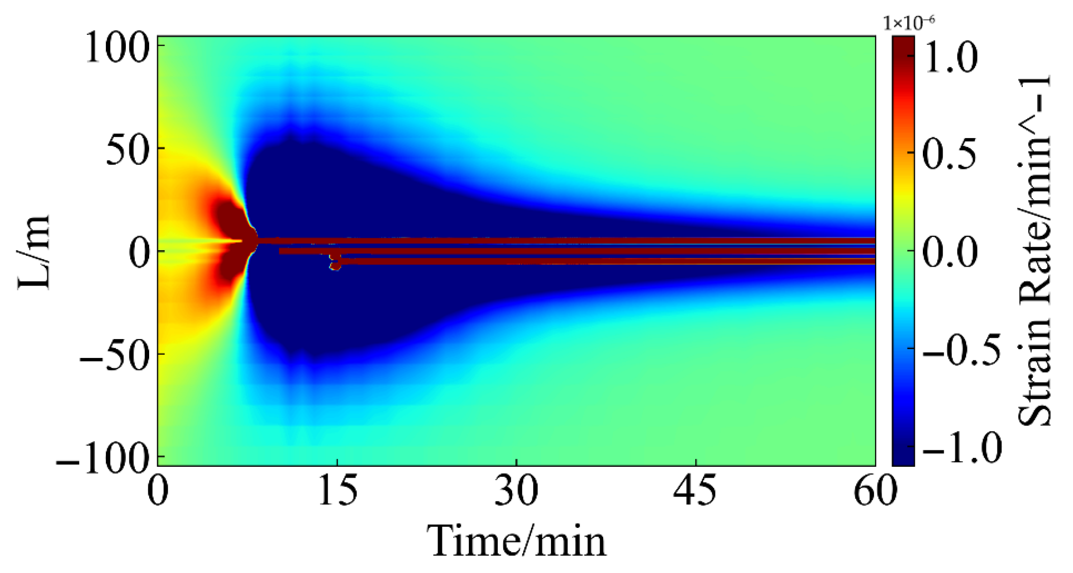
Among these techniques, the low-frequency component of the DAS response recorded in a horizontal neighbor-well (LF-DAS) has proved particularly effective for monitoring fracture propagation [13,14]. When a vertical hydraulic fracture approaches the fiber deployed in a horizontal neighbor-well, the LF-DAS strain-rate waterfall plot exhibits a characteristic tensile heart-shaped pattern (Figure 1), with a stable tensile band at the fracture-hit location and compressive zones on both sides due to the stress-shadow effect [13,15,16,17,18].
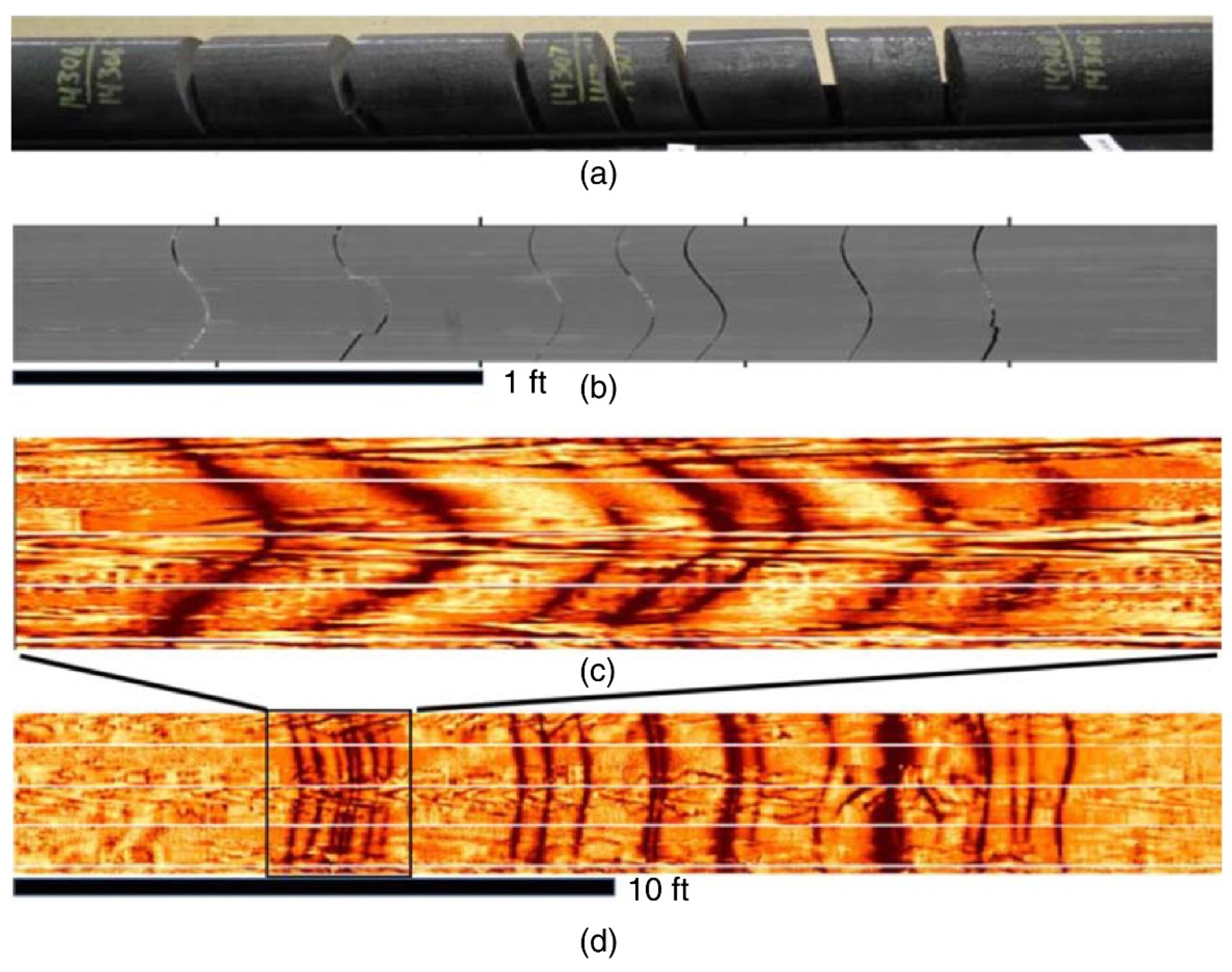
Field coring campaigns at the HFTS-2 site and other test sites have revealed that hydraulic fractures frequently propagate as densely clustered swarms rather than as isolated single fractures (Figure 2) [19,20,21,22]. Reported analyses indicate that a substantial proportion of the documented inter-fracture spacings are less than 0.3 m [19,22], well below the gauge lengths commonly used in field LF-DAS deployments (typically 7–15 m) [23]. Because each DAS sensing channel reports the axial strain rate averaged over the gauge-length interval, the measurement acts as a spatial low-pass filter that merges closely spaced fracture features into a single broad tensile band, making individual fractures indistinguishable [24]. Shortening the gauge length to improve resolution sacrifices signal-to-noise ratio (SNR) and amplifies coupling artefacts, whereas lengthening it further merges adjacent features, producing a resolution–SNR trade-off that remains one of the central bottlenecks of current LF-DAS fracture monitoring [13,23].
Considerable progress has been made in the interpretation and inversion of LF-DAS strain-rate responses. Early empirical studies established that the heart-shaped pattern and its spatial extent can be used to identify fracture arrival, propagation direction, and approximate distance, providing valuable engineering intuition for qualitative fracture characterization [13,15,16,17,18]. Building on these observations, a number of physics-based forward models and inversion frameworks have been developed. Liu et al. [15,25,26] proposed a DDM-based forward model and a Green’s-function fracture-width inversion approach. Tan et al. [27] coupled a fracturing simulator with a finite-element solver, Gurjao et al. [28] derived an analytical strain model for two-dimensional fracture propagation, Srinivasan et al. [29] formulated a corresponding model for vertical neighbor-wells, and Leggett et al. [30] introduced a fracture-length inversion method. More recently, Tu et al. [31] proposed an optimization-based inversion framework combining Green’s functions with Sneddon-type width functions. These methods have made quantitative fracture-geometry estimation from LF-DAS data increasingly feasible; however, they generally treat the gauge length as a fixed instrument property and have not explicitly targeted the resolution loss caused by gauge-length averaging in dense-cluster scenarios [15,25,26,27,28,29,30,31].
In parallel, coupled fluid–geomechanical simulation frameworks have been developed to generate synthetic LF-DAS responses and to investigate the sensitivity of interpretation to fracture interactions and stress shadows [32]. While such simulations enhance mechanistic understanding, their computational cost constrains multi-scenario iteration and near-real-time deployment. In a complementary direction, Ma et al. [33] demonstrated that DAS-recorded microseismic reflections can provide independent fracture-geometry constraints, and laboratory-scale fiber-optic monitoring of hydraulic fracturing has also been reported [34]. These studies broaden the interpretive toolkit but have not directly addressed the gauge-length-averaging-induced spatial resolution limitation that is the focus of the present work.
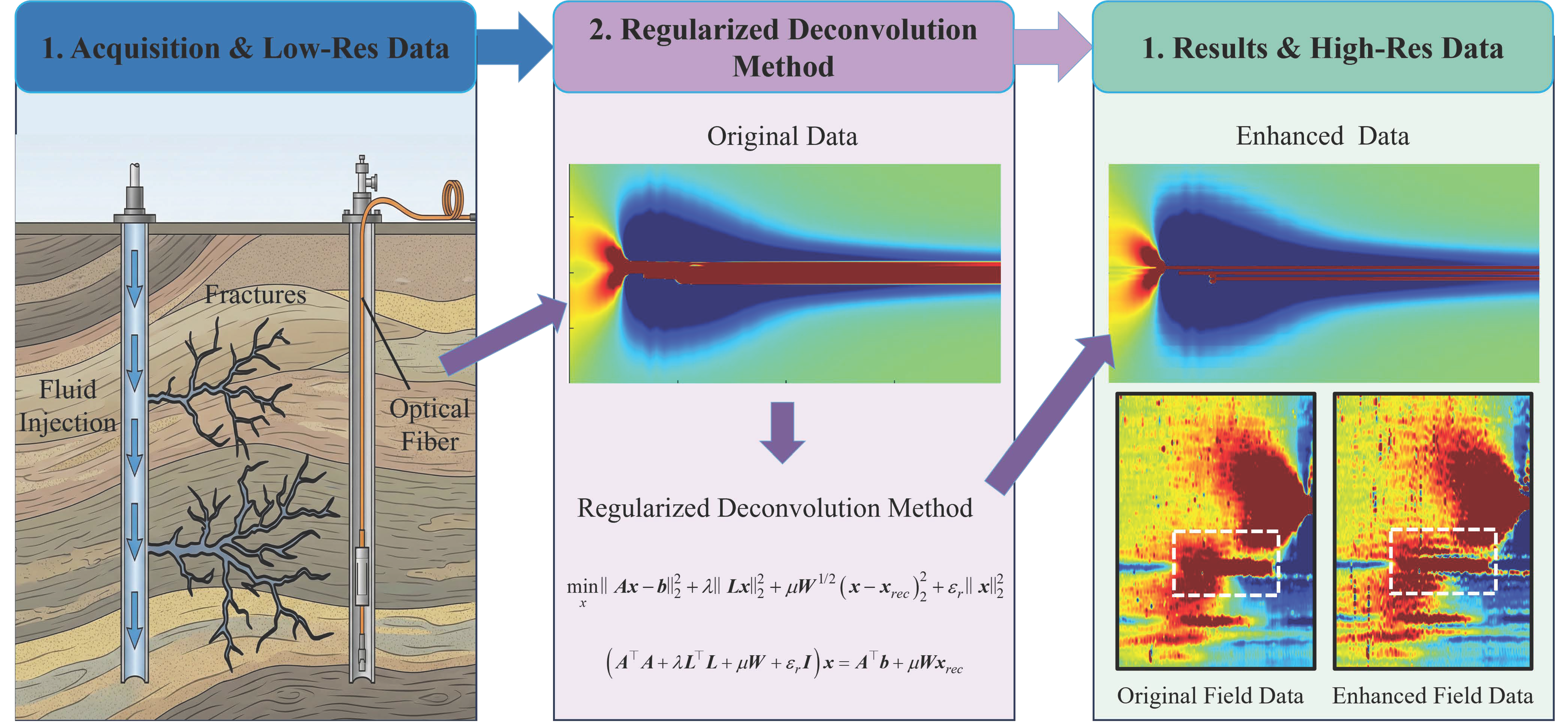
To address this resolution bottleneck, this study proposes a super-resolution enhancement framework for neighbor-well LF-DAS data based on a regularized inversion method. The gauge-length spatial averaging is formulated as an explicit convolution operator, and the super-resolution recovery is cast as an inverse problem under noisy conditions. Second-order Tikhonov regularization with L-curve-based automatic parameter selection is employed, together with a recursive prior that stabilizes the solution in low-coverage and high-noise regions [35]. An efficient semi-analytical forward model based on the Boussinesq elastic half-space solution is also developed for multi-fracture validation and sensitivity analysis [36]. The objective is to advance the effective spatial resolution of neighbor-well LF-DAS from the gauge-length scale (typically 7–15 m) down to the sample-spacing scale (approximately 1 m), and to quantify the effects of gauge length, sample spacing, and noise level on the achievable resolution. The three key contributions are: (i) a regularized inversion framework that explicitly inverts the gauge-averaging operator; (ii) an efficient semi-analytical multi-fracture forward model consistent with the LF-DAS measurement definition; and (iii) a systematic validation framework including quantitative synthetic benchmarks, noise-sensitivity analysis, baseline comparison, and field-scale evaluation on the HFTS-2 dataset.
The remainder of this paper is organized as follows. Section 2 develops the regularized inversion method and the semi-analytical forward model. Section 3 presents quantitative validation including noise-sensitivity and baseline-comparison studies. Section 4 and Section 5 discuss parameter sensitivity and field application to HFTS-2 data, respectively, and Section 6 concludes the paper.

2. Materials and Methods

In this section, we present an integrated methodological framework for neighbor-well LF-DAS-based monitoring of closely spaced hydraulic fractures, consisting of a resolution enhancement module and an efficient forward-modeling module. First, we formulate the DAS measurement as a gauge-length spatial averaging process (i.e., a convolution of the true axial strain-rate field with a gauge-length kernel), which fundamentally limits the ability to resolve adjacent fracture-induced responses. Based on a discretized representation of the gauge-length overlap, the resolution enhancement problem is recast as a noisy inverse problem and solved using a regularized inversion method that combines second-order Tikhonov smoothing with a lightweight recursive prior and observability-based adaptive weighting, thereby improving robustness under low-signal-to-noise conditions. Second, to enable rapid and scalable prediction of neighbor-well strain responses for multi-cluster fracture propagation, we employ a semi-analytical elastic half-space formulation built upon fracture-surface equivalent load inversion, Boussinesq kernels, coordinate transformations, and linear superposition, while maintaining consistency with the gauge-length definition of DAS strain. Together, these two components provide a computationally efficient and physically consistent basis for high-resolution inversion and forward simulation of neighbor-well LF-DAS responses in clustered-fracture scenarios.

2.1. Resolution Enhancement Model for Neighbor-Well LF-DAS

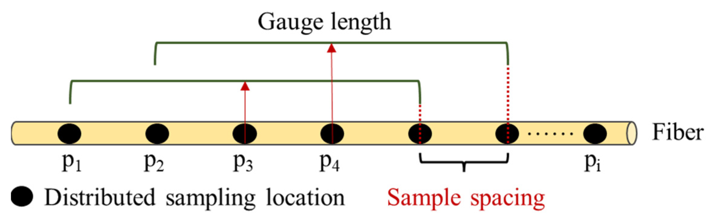
The application of LF-DAS in hydraulic fracturing monitoring is fundamentally based on its capability to measure phase variations along the optical fiber and subsequently convert them into axial strain responses at the fiber sensing locations [13,37]. It should be emphasized that DAS measurements do not represent pointwise strain responses. Instead, the recorded signal corresponds to the spatially averaged axial strain rate of the fiber over a predefined gauge length [38]. As illustrated in Figure 3, the discrete sampling positions along the fiber (i.e., DAS channels) are located at the centers of their corresponding gauge-length intervals. Consequently, the measured LF-DAS signal inherently reflects a convolution of the true strain field with a spatial averaging kernel determined by the gauge length, which constitutes the fundamental source of resolution degradation in closely spaced fracture monitoring.
In field applications of LF-DAS for hydraulic fracturing monitoring, the sample spacing is commonly set as an integer fraction or multiple of the gauge length, such that the gauge length can be treated as a spatial averaging window covering an integer number of sensing channels [23]. This configuration not only facilitates spatial stacking and noise suppression in data processing, but also satisfies the basic requirement of spatial oversampling for LF-DAS measurements while maintaining an adequate signal-to-noise ratio.
Accordingly, the following reasonable assumptions are adopted in the development of the proposed resolution enhancement method for neighbor-well fiber-optic strain monitoring:
  • Negligible fiber–formation slip: No significant relative slip is assumed between the fiber-optic cable and the surrounding formation, and the measured LF-DAS response is therefore regarded as a valid representation of the true formation strain-rate response;
  • Gauge-length averaging: The measurement at each sensing channel is assumed to be equivalent to the axial strain-rate average over the gauge-length interval centered at that channel location;
  • Integer relationship between gauge length and sensor spacing: The gauge length is assumed to be an integer multiple of the sample spacing.
Three additional effects that may influence real-world applicability deserve explicit mention. Fiber–formation slip: the fiber is assumed to be fully coupled to the formation because, in all field cases considered in this work (including the HFTS-2 deployment), the fiber cable is cemented behind casing, the standard engineering configuration for quasi-static LF-DAS monitoring of hydraulic fracturing. We acknowledge that residual slip at the cement–cable or cement–formation interfaces may introduce a systematic bias in the absolute strain amplitude; however, the feature-detection metrics employed in this study (number of distinguishable tensile features, peak position, and peak full-width at half-maximum) depend primarily on relative amplitudes and spatial derivatives of the signal, and are therefore less sensitive to such a bias than an absolute-amplitude interpretation would be. A dedicated quantification of fiber-coupling effects is outside the scope of the present work and is noted as a direction for future study. Reservoir heterogeneity: meter-scale heterogeneity of the elastic properties affects absolute strain amplitudes but is partially averaged out because neighbor-well LF-DAS responses are dominated by far-field elastic deformation; strong heterogeneity is therefore a known source of amplitude uncertainty but has a limited effect on the spatial localization and count of tensile features. Fracture non-linearity: plastic deformation and process-zone effects are concentrated near the fracture tip and within a few tip-lengths; at the neighbor-well distances considered here (tens of meters), linear elasticity is a reasonable approximation. We acknowledge that all three effects deserve dedicated future studies in conjunction with coupled fluid–solid–damage modeling.
To elucidate the fundamental mechanism of resolution enhancement, an idealized noise-free scenario is first considered. The gauge-length interval G associated with each sensing channel is uniformly discretized into N subintervals with a length equal to the sample spacing dl, where N = G/dl. For an arbitrary sensing channel i, the corresponding fiber-optic measurement can then be expressed as the discrete average of the axial strain rate over the gauge-length interval, namely,
b i = 1 N 1 N x j dl
where bi denotes the measured strain-rate response at sensing channel i, and xj represents the average axial strain rate over the j-th subinterval within the gauge-length window.
As illustrated in Figure 3, the gauge-length intervals associated with adjacent sensing channels partially overlap. Consequently, the measurements from neighboring channels share a portion of the underlying subinterval strain-rate responses. The strain-rate contributions from the non-overlapping subintervals between channel i + 1 and channel i can therefore be expressed as
x new = 1 dl ( N b i + 1 2 N x j dl )
where bi+1 denotes the measured strain-rate response at sensing channel i + 1, and N represents the number of subintervals within the gauge-length window, defined as N = G/dl. Owing to the fact that formation strain induced by fracture propagation decays rapidly with increasing distance from the fracture, the strain-rate contribution associated with the subinterval corresponding to the far-end sensing channel (Channel 1) can be reasonably approximated as
x 1 x j x N b 1
By successively applying Equation (2), the strain-rate magnitude of each subinterval can be solved in a recursive manner, thereby enabling the effective enhancement of spatial resolution from the gauge-length scale G to the sensor-spacing scale dl.
However, field LF-DAS measurements are typically contaminated by significant noise. Direct application of the aforementioned differential recursive scheme would therefore lead to error accumulation and noise amplification, resulting in pronounced distortions in the inverted strain-rate field. To address this issue, the resolution enhancement problem is reformulated as an inverse problem under noisy observations, in which the following strategies are introduced:
  • Second-order difference Tikhonov regularization is employed to suppress high-frequency noise and stabilize the ill-posed solution;
  • Recursive prior information is incorporated to provide physically consistent weak constraints in end segments and low-coverage regions;
  • Observability-based weighting W is constructed according to segment-level coverage, such that prior constraints are strengthened in poorly covered regions while data fidelity dominates in well-covered regions, thereby improving robustness and interpretability under high-noise conditions.
In neighbor-well DAS measurements, the recorded response at each fiber sensing location p i ( i = 1 , , M ) corresponds to the gauge-length-averaged axial strain rate over an interval of length G. Let the unknown spatial field to be inverted be denoted by x ( l ) , where l represents the coordinate along the wellbore axis (in meters). Under noisy measurement conditions, the fiber-optic observation at an arbitrary sensing channel p i can be expressed as
b i = 1 G p i G 2 p i + G 2 x ( l ) dl + e i
where x ( l ) denotes the continuous distribution of the axial strain-rate response within the gauge-length interval associated with sensing channel i, and e i represents the measurement noise. The gauge-length coverage corresponding to an arbitrary sensing channel is uniformly partitioned into N subintervals, each with a center located at l j , where the step size dl equals the sample spacing. Let x = x 1 , , x N denote the subinterval-averaged strain-rate value, and let b = b 1 , , b M represent the observation vector. The discrete measurement relationship can then be written as
b = A x + ε
A i j full = o v e r l a p l j Δ l 2 , l j + Δ l 2 , p i G 2 , p i + G 2 Δ l
where A denotes the overlap matrix, o v e r l a p ( [ a , b ] , [ c , d ] ) = max ( 0 , min ( b , d ) max ( a , c ) ) .
Let r i = j A i j full . The matrix A i j full is then normalized in a row-wise manner to preserve the physical consistency of a gauge-length weighted average, i.e.,
A i j = A i j full r i ,   j = 1 N A i j = 1
Accordingly, the discrete fiber-optic observation at an arbitrary sensing channel p i can be written as
b i = j = 1 N A i j x j + e i , i = 1 , , M
A smoothing matrix L R ( N 2 ) × N is constructed using the second-order finite-difference scheme, i.e.,
( L x ) k = x k 2 x k + 1 + x k + 2 , k = 1 , , N 2
The noise-contaminated optimization problem is reformulated as an inverse problem using the Tikhonov regularization framework [24,35], i.e.,
min x A x b 2 2 + λ L x 2 2 + ε r x 2 2
The corresponding sparse system of equations can be written as
A A + λ L L + ε r I x = A b
where λ denotes the Tikhonov smoothing parameter and ε r represents a small ridge term introduced to improve numerical stability. It should be noted that, in regions with insufficient coverage (e.g., end segments or missing channels) or under low-signal-to-noise ratio conditions, relying solely on the Tikhonov regularization term may introduce plateau-like artifacts in the inverted field.
To mitigate this issue, a lightweight recursive solution x rec is constructed and incorporated as a prior. Specifically, the first K sensing channels are selected, and a least-squares problem is solved over the subintervals covered by these channels to obtain an initial estimate for the leading segment. Subsequently, the solution is propagated progressively from near to far along the sensing direction. For a given sensing channel p i , the set of subintervals covered by its gauge-length window is identified as
Ω i = j A i j > 0
The indices within Ω i that have not yet been estimated are partitioned into contiguous blocks. Only the block B i that is immediately adjacent to the propagation direction is updated at the current step, while the remaining contribution is distributed so as to preserve consistency with the gauge-length-averaged measurement at the sensing channel.
j Ω i A i j x j b i x j B i = b i j Ω i A i j j Ω i B i A i j x j j B i A i j
The forward and backward recursive estimates obtained by propagating along the fiber from the near end to the far end and vice versa are combined by segment-wise averaging. Any remaining incomplete segments are filled using nearest-neighbor interpolation, yielding the prior estimate x rec . Based on this estimate, the coverage degree and the degree of insufficient coverage are subsequently defined as
c j = i = 1 M A i j
w j = 1 c j max k c k [ 0 , 1 ]
An adaptive prior-weighting coefficient μ is then defined to ensure that the contribution of the prior term varies consistently with both the local coverage degree and the noise level.
μ j = μ 0 w j w ¯ γ σ ^ σ 0 β , γ , β 0
where γ and β are the exponents controlling the influence of the segment-level coverage-based prior weighting, σ ^ denotes a robust estimate of the observation noise scale, σ 0 is a reference noise scale, and μ 0 represents the reference weight assigned to the prior term.
By treating the recursive estimate as a flexible prior and harmonizing its contribution through a dual adaptive weighting scheme based on coverage degree and noise level, a unified objective function is constructed as follows:
min x A x b 2 2 + λ L x 2 2 + μ W 1 / 2 x x rec 2 2 + ε r x 2 2
where W = d i a g w 1 , , w N denotes the segment-level weighting matrix. Accordingly, the associated normal equations can be derived as
A A + λ L L + μ W + ε r I x = A b + μ W x rec
Solving the above normal equations yields the enhanced-resolution distribution of the subinterval strain rates, denoted by x .
Throughout the rest of this paper, we refer to this combined scheme, gauge-averaging operator inversion + second-order Tikhonov smoothing + recursive prior as the regularized inversion method.
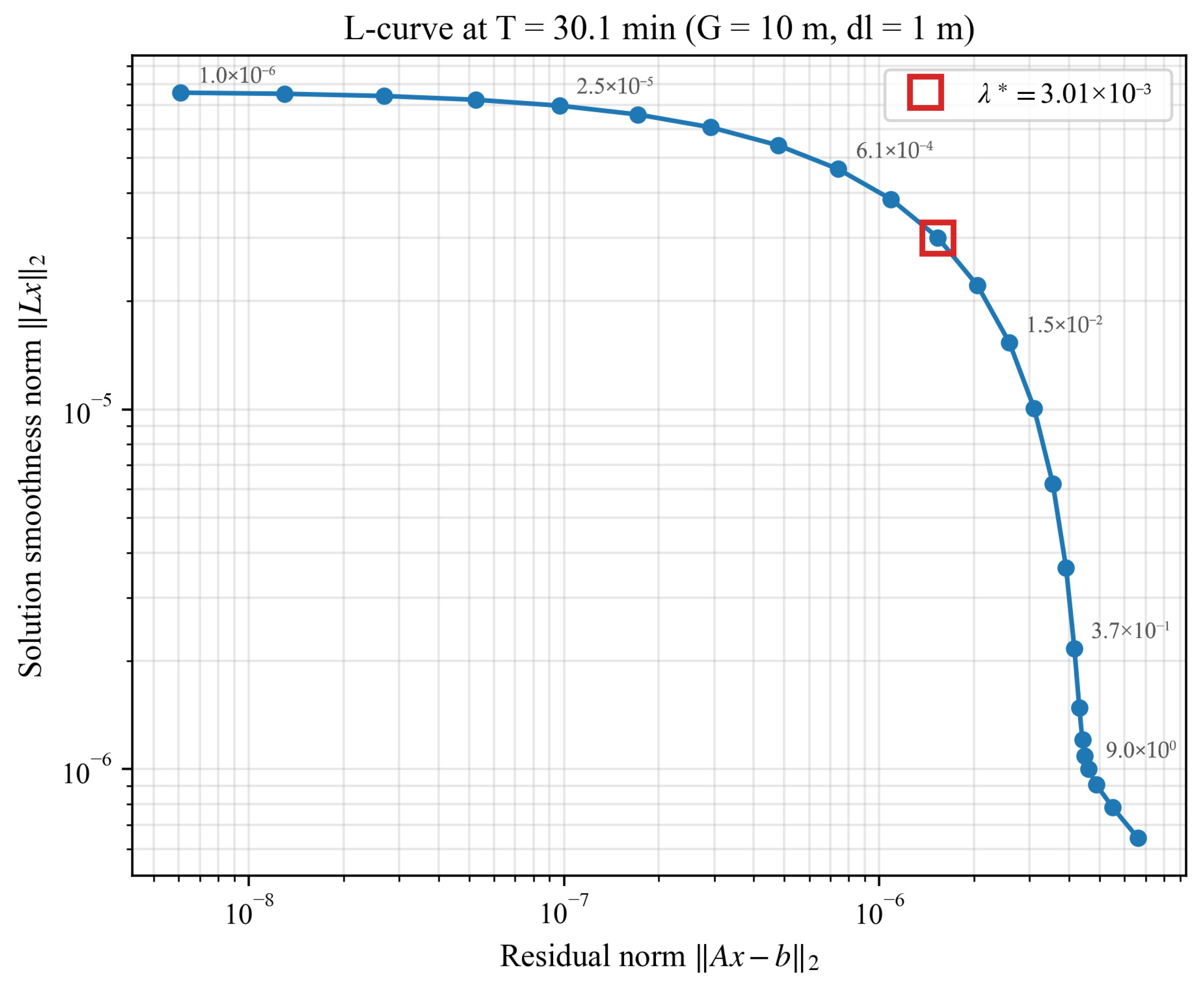
The trade-off between data fidelity and spatial smoothness inside the regularized inversion method can be visualized by an L-curve construction. For a logarithmic sweep of candidate smoothing weights λ , the data-misfit norm A x b 2 and the second-order smoothness norm L x 2 are computed and plotted in log–log coordinates (Figure 4). The trajectory exhibits the characteristic L shape; the corner of the curve, identified automatically as the point of maximum log-domain curvature, marks the trade-off optimum. For the synchronous-fracture benchmark at T = 30.1 min, this corner is located at λ ≈ 3.01 × 10⁻³. Once identified for a given acquisition geometry, the corner value is reused for every time step at no extra cost. In practice, the optimal λ is governed by two factors: the structure of the overlap matrix A, which depends solely on the acquisition geometry (G, dl, and the channel layout), and the noise floor of the measurement. Because neither factor changes during a continuous pumping stage, a single L-curve evaluation on any representative time slice yields a λ* that remains valid for every subsequent time step of the same dataset. Recomputation is only necessary when the acquisition geometry or noise environment changes, for instance between different well pairs or field campaigns. The complete procedure is summarized in Algorithm 1; the definitions and default values of all model parameters are collected in Table 1.
Algorithm 1. Regularized inversion method.
Input: measurements b ∈ RM, gauge length G, sample spacing dl, initial channels K (default 3), smoothing weight λ (from L-curve, Figure 4), ridge stabilizer ε
Output: high-resolution strain-rate field x ∈ℝ^ Ntot, where Ntot = (Lmax − Lmin)/dl
 
1. Build the gauge-averaging overlap matrix A (M × Ntot) from the acquisition geometry.
Normalize A row-wise so that each row sums to 1.
2. Initialize the leading K channels by least-squares: Alead xlead = blead.
3. for i = K, K + 1, …, M − 1 (near-to-far propagation pass):
Identify sub-segments covered by channel i but not yet estimated;
Update the contiguous block on the propagation side so that
the gauge-averaged value over channel i matches observation bi.
end for
4. for i = MK + 1, …, 1 (far-to-near propagation pass):
Repeat step 3 in the opposite direction.
end for
5. Fuse the two passes by segment-wise averaging.
Fill remaining incomplete sub-segments by nearest-neighbor interpolation.
6. (Optional, recommended if SNR < 20 dB)
Apply wavelet pre-denoising along the fiber axis:
db4 basis, soft thresholding, MAD-based universal threshold.
7. Assemble the Tikhonov normal equations:
A A + λ L L + μ W + ε r I x = A b + μ W x r e c
where  x r e c is the fused propagation-pass estimate from step 5.
8. Solve for x via sparse Cholesky factorization.
return x

2.2. Efficient Semi-Analytical Forward Model for Clustered Fractures

Mao et al. [36] developed an efficient semi-analytical forward model for neighbor-well fiber-optic strain responses induced by hydraulic fracture propagation. By maintaining physical consistency, the model significantly reduces the computational cost associated with neighbor-well DAS forward simulations and can be readily coupled with various fracture propagation models. Building upon this framework, the present study further extends the model to clustered fracture propagation scenarios by incorporating coordinate transformation techniques and the principle of linear elastic superposition. The primary motivation for adopting a semi-analytical formulation lies in the intrinsic characteristics of clustered fractures. Compared with grid-based numerical approaches, clustered fracture systems are typically characterized by small inter-fracture spacing and a large number of fractures. Conventional mesh-based methods therefore require substantial local mesh refinement in the vicinity of fractures, causing the computational cost to increase rapidly with fracture density. In contrast, the proposed semi-analytical approach does not rely on spatial discretization of the solution domain and can thus maintain high computational efficiency and favorable scalability even under conditions involving closely spaced fractures.
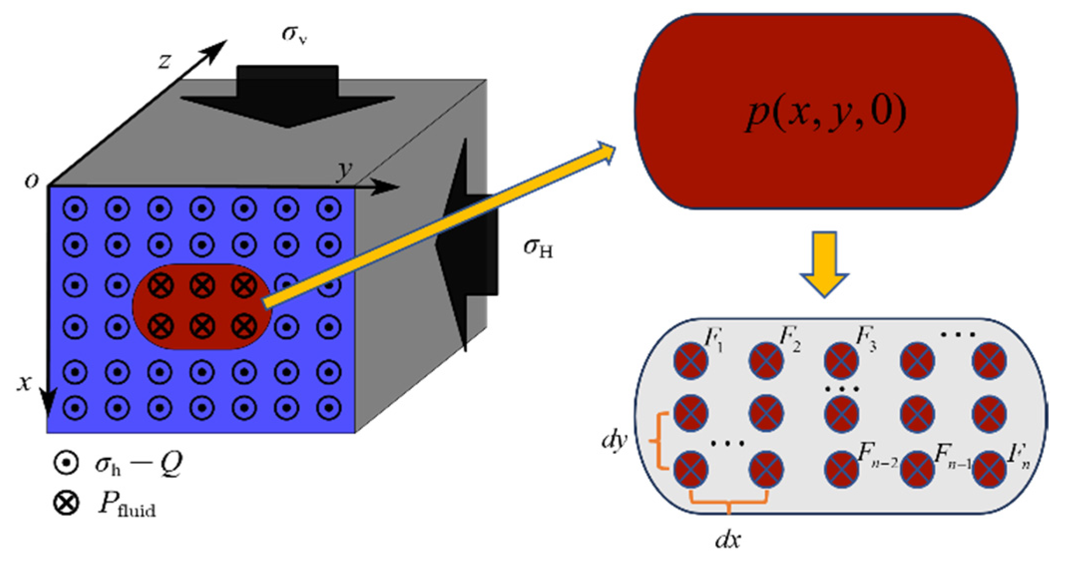
In the formulation of neighbor-well fiber-optic strain responses, Mao et al. proposed an approach in which the fracture-surface pressure is discretized into a set of equivalent concentrated forces (point loads). By enforcing the displacement boundary conditions on the fracture surfaces, the distribution of these equivalent loads surrounding the fracture plane is inverted. The displacement field of the elastic half-space induced by the equivalent point loads is then superposed using the Boussinesq solution, from which the strain response along the neighboring fiber-optic cable can be obtained (Figure 5).
The fundamental assumptions underlying this semi-analytical model are summarized as follows:
  • The reservoir is modeled as a homogeneous, isotropic, linear elastic medium;
  • Perfect mechanical coupling is assumed between the formation and the fiber-optic monitoring well, with no relative slip at the interface;
  • Body forces are neglected;
  • The in situ stress state prior to fracturing is taken as the reference configuration, with the initial displacement and strain fields assumed to be zero.
For a homogeneous, isotropic elastic half-space subjected to a normal concentrated force, the displacement components at an arbitrary point within the half-space, expressed in a cylindrical coordinate system, can be obtained from the classical Boussinesq solution [39] as follows:
u ρ F = ( 1 + v ) F 2 π E R ρ z R 2 ( 1 2 v ) ρ R + z u θ F = 0 u zF = ( 1 + v ) F 2 π E R 2 ( 1 v ) + z 2 R 2
Based on the prescribed displacement boundary conditions around the fracture surface u z = 0 [40], the distribution of the equivalent stress Q acting in the vicinity of the fracture can be determined from the following relationship:
u z 1 ( F 1 ) + u z 1 ( F i ) + u z 1 ( F n ) + u z 1 ( Q 1 ) + u z 1 ( Q i ) + u z 1 ( Q m ) = 0 u z 2 ( F 1 ) + u z 2 ( F i ) + u z 2 ( F n ) + u z 2 ( Q 1 ) + u z 2 ( Q i ) + u z 2 ( Q m ) = 0                  u z ( m 1 ) ( F 1 ) + u z ( m 1 ) ( F i ) + u z ( m 1 ) ( F n ) + u z ( m 1 ) ( Q 1 ) + u z ( m 1 ) ( Q i ) + u z ( m 1 ) ( Q m ) = 0 u z m ( F 1 ) + u z m ( F i ) + u z m ( F n ) + u z m ( Q 1 ) + u z m ( Q i ) + u z m ( Q m ) = 0
Accordingly, the displacement response at an arbitrary point within the elastic half-space can be expressed as the superposition of the contributions from all equivalent loads, i.e.,
u x = i = 1 n u x F i + i = 1 m u x Q i u y = i = 1 n u y F i + i = 1 m u x Q i u z = i = 1 n u z F i + i = 1 m u x Q i
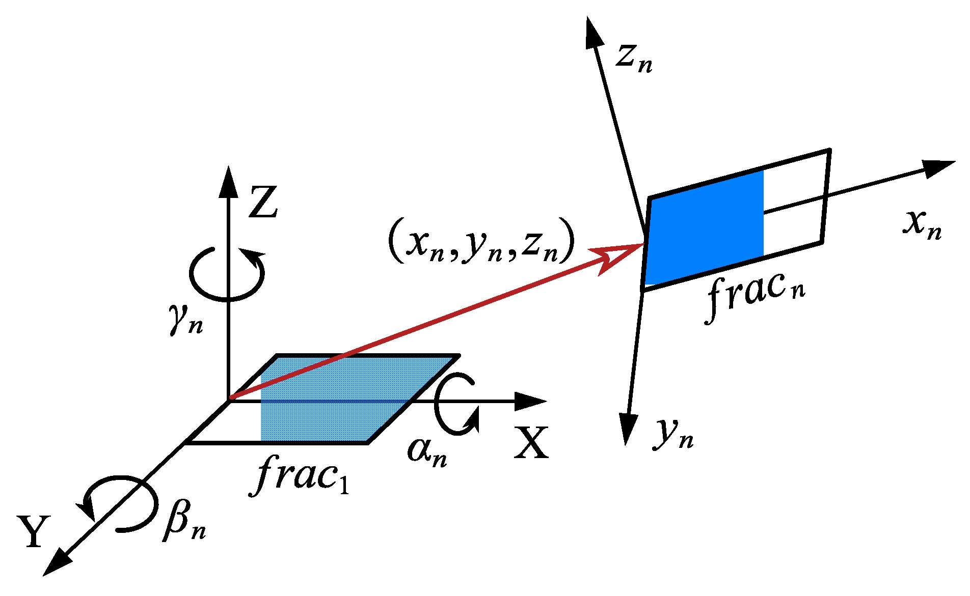
For scenarios involving the propagation of multiple fractures, a local coordinate system is established for each individual fracture, while a unified semi-analytical kernel derived for a single fracture is reused in a consistent manner. Specifically, the local coordinate system associated with the n -th fracture is obtained from the global coordinate system through successive rotations about the x -, y -, and z -axes by angles α n , β n , and γ n , respectively (Figure 6).
The rotation matrix that transforms the local coordinate system of the n -th fracture to the global coordinate system can be written as
R n l g = R x α n R y β n R z γ n
R x α n = 1 0 0 0 cos α n sin α n 0 sin α n cos α n
R y β n = cos β n 0 sin β n 0 1 0 sin β n 0 cos β n
R z γ n = cos γ n sin γ n 0 sin γ n cos γ n 0 0 0 1
In the local coordinate system of the n -th fracture, the displacement induced by this fracture, u k l , n , is computed using Equation (22). The corresponding displacement expressed in the global coordinate system is then given by
u k g , n = R n l g u k l , n
Under the small-deformation assumption of linear elasticity, the superposition principle holds, and the total displacement field induced by multiple fractures can be expressed as
u total , k g = n = 1 N frac u k g , n
In field LF-DAS measurements, the axial strain recorded at each sensing channel is defined as the gauge-length-averaged axial strain over an interval of length G. To ensure consistency with this measurement definition, the axial strain of the fiber is computed herein using a displacement-difference formulation. Specifically, along the fiber direction, the displacement difference between two points separated by a distance G is evaluated and subsequently divided by G to obtain the gauge-length-averaged axial strain, i.e.,
ε = u i + G 2 u i G 2 G
Accordingly, the fiber-optic axial strain rate can be expressed as
ε ˙ = ε d t = ε n + 1 ε n Δ t
By applying Equations (21) and (29), the neighbor-well fiber-optic strain-rate response induced by fracture propagation can be obtained.
In summary, the proposed approach employs the Boussinesq half-space solution as the analytical kernel and integrates fracture-surface equivalent load inversion with coordinate transformation and stress/displacement superposition, enabling efficient evaluation of neighbor-well fiber-optic strain-rate responses under clustered fracture propagation scenarios. As the solution does not require spatial meshing of the computational domain, the method avoids the substantial increase in computational cost that is typically associated with mesh refinement when dealing with complex multi-fracture systems. Consequently, it offers high computational efficiency and favorable applicability for practical engineering analyses.
The semi-analytical forward model used in this manuscript is an extension of the model introduced by Mao et al. [36], in which the model has already been validated against two independent reference benchmarks. First, for a penny-shaped fracture, the stress field computed by the semi-analytical method was compared against the classical Sneddon analytical solution at four fiber-to-fracture distances df = 2, 6, 10 and 16 m. The comparison shows that while at small df the semi-analytical result departs from Sneddon due to Saint-Venant boundary effects close to the fracture plane, the agreement becomes excellent once df ≥ 10 m, which is the distance range representative of field LF-DAS acquisition and for which the relative stress-field error falls well within engineering tolerances. Second, for a vertical elliptical fracture monitored by a horizontal neighbor well, the semi-analytical result was benchmarked against the displacement-discontinuity method (DDM) implementation of Liu et al. [15]; the characteristic heart-shaped strain-rate response predicted by the two approaches was found to be strongly consistent, confirming the applicability of the semi-analytical approach to the multi-fracture cases considered in the present study.

3. Validation

3.1. Multi-Fracture Benchmark

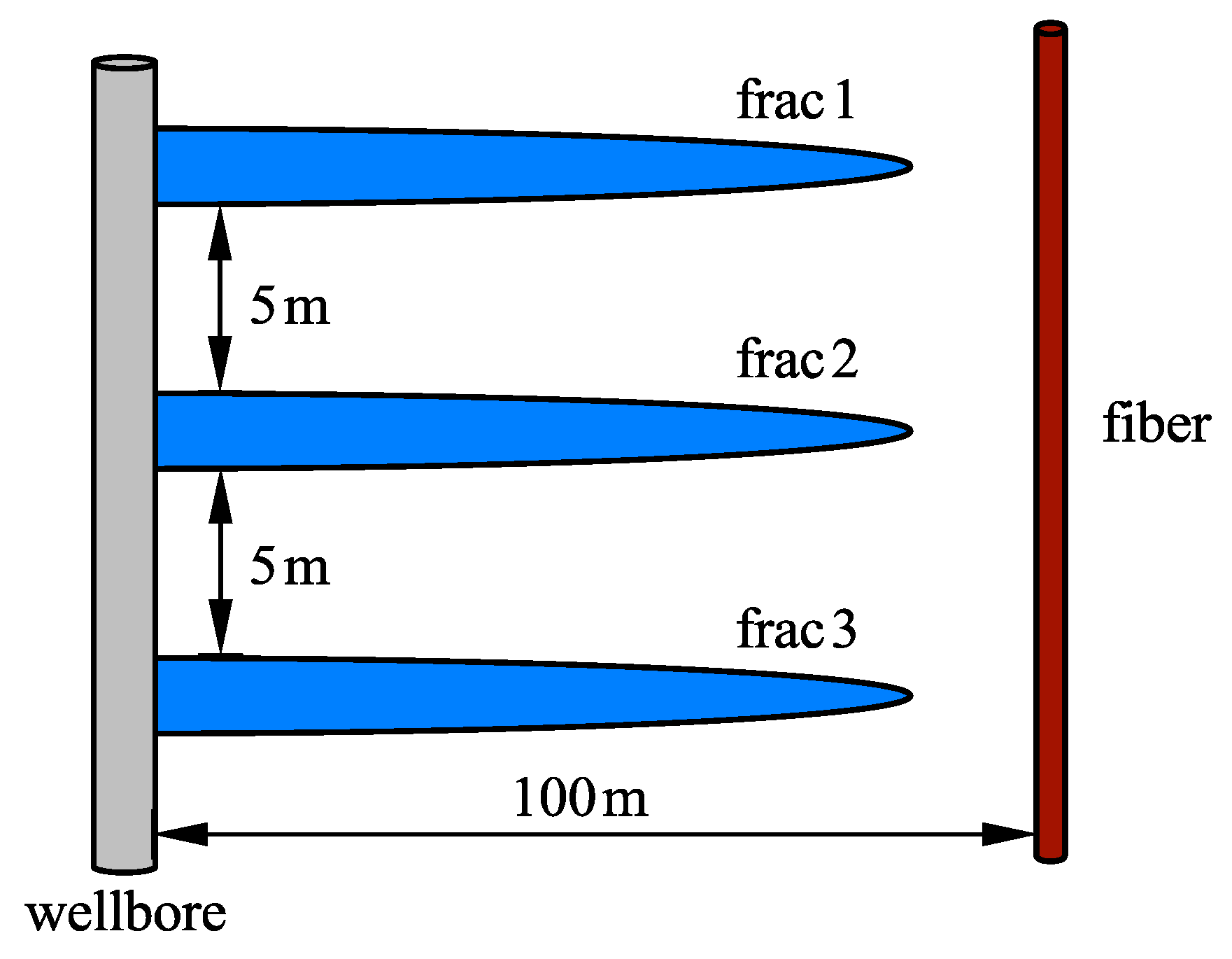
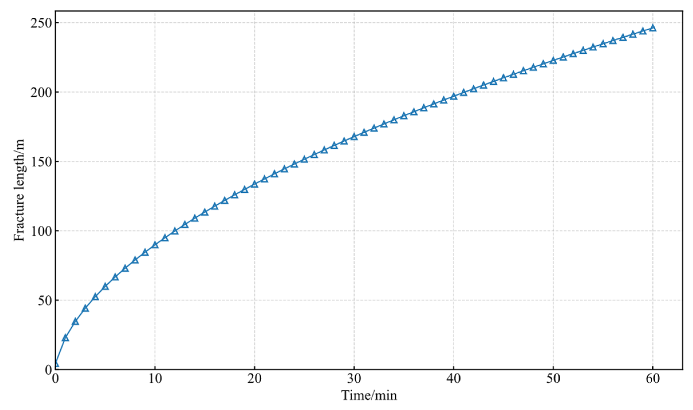
To validate the proposed spatial resolution-enhancement method for neighbor-well LF-DAS monitoring, a numerical benchmark case is designed in which a horizontal neighbor-well is used to monitor the propagation of three hydraulic fractures. The distance between the treatment well and the horizontal monitoring well is set to 100 m. The three fractures are arranged parallel to each other along the wellbore direction, with an inter-fracture spacing of 5 m. The configuration of the monitoring well is illustrated in Figure 7, where the fiber-optic monitoring well is highlighted in red. Fracture propagation is simulated using the PKN model [41] (Figure 8). The resulting fracture geometry parameters are then incorporated into the semi-analytical forward model developed in this study to generate neighbor-well fiber-optic strain-rate responses under two gauge-length conditions, namely G = 1 m and G = 10 m. The response obtained with G = 1 m is taken as a high-resolution reference solution, against which the consistency and accuracy of the resolution-enhanced results are evaluated. The fracture propagation parameters and formation properties used in the numerical simulations are summarized in Table 2.
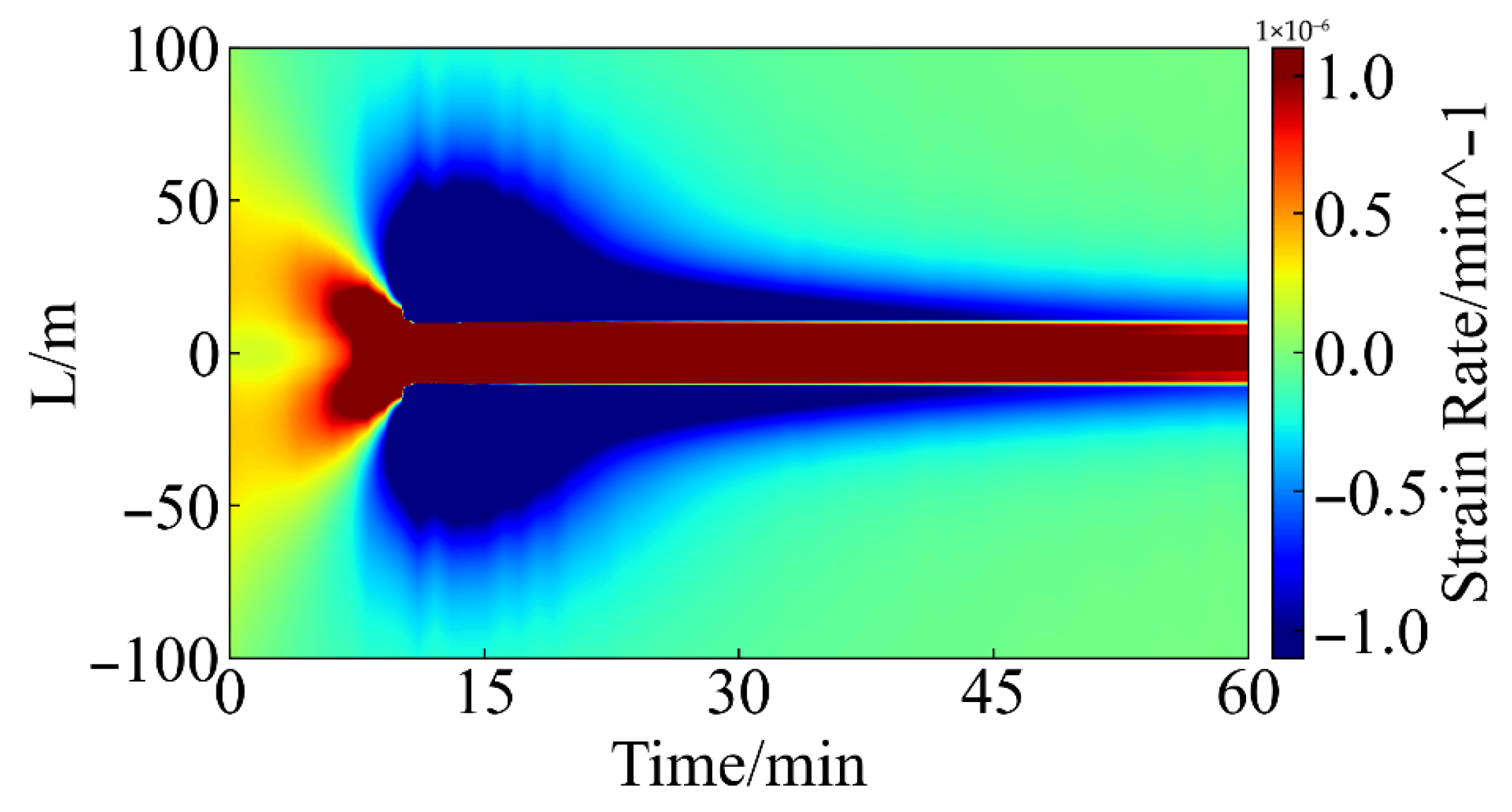
Figure 9 and Figure 10 present the strain-rate waterfall plots obtained under gauge-length conditions of G = 10 m and G = 1 m, respectively. For the G = 1 m case, the strain-rate response is dominated by a single tensile “heart-shaped” zone accompanied by a corresponding tensile band. The emergence of the heart-shaped pattern indicates that the fracture propagation front reaches and intersects the monitoring well, which occurs at approximately 12 min in this benchmark case. When the gauge length is increased to G = 10 m, which is significantly larger than the inter-fracture spacing of 5 m, the LF-DAS measurement effectively performs spatial averaging over the gauge-length interval. As a result, the responses induced by multiple fractures become spatially aliased, and the individual fracture contributions can no longer be distinguished in the waterfall plot. Consequently, only a single dominant tensile band is observed.
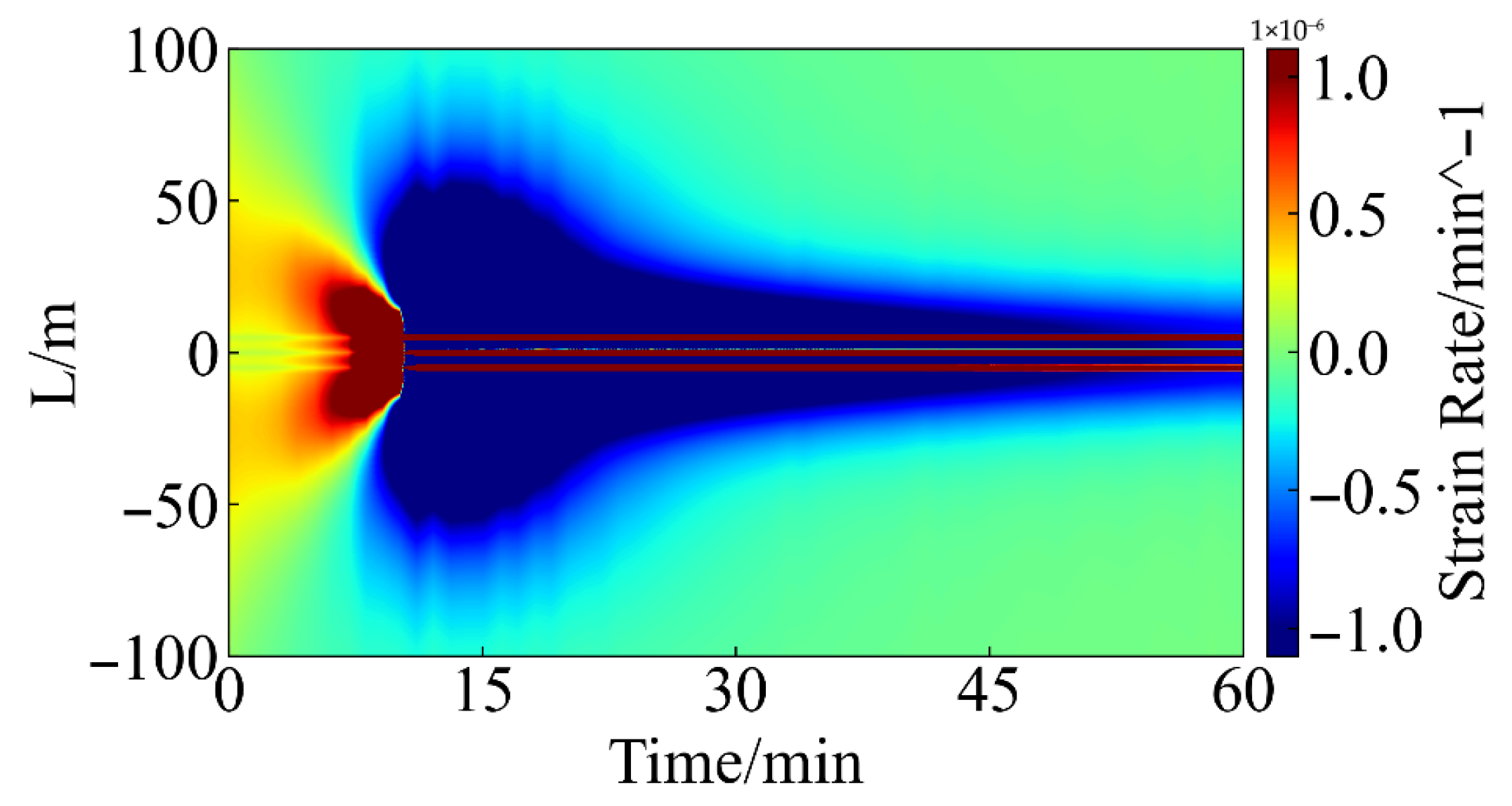
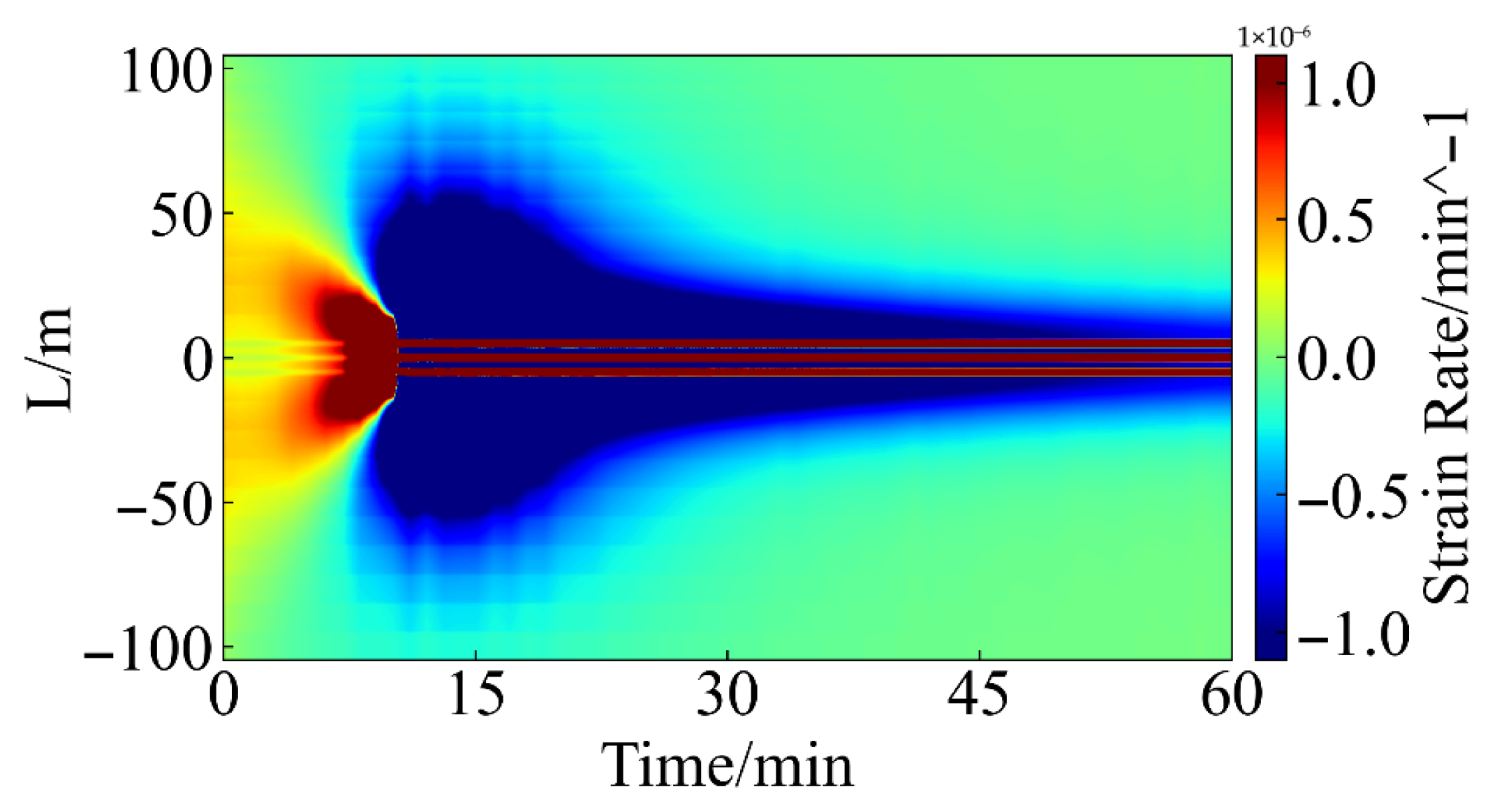
In contrast, under the high-resolution condition of G = 1 m, the waterfall plot is capable of resolving the coupled heart-shaped responses associated with the three fractures and forms three distinct tensile bands after fracture hit (Figure 10), which is fully consistent with the prescribed fracture geometry. Furthermore, the strain-rate data obtained with G = 10 m are processed using the proposed resolution enhancement method, yielding the enhanced-resolution waterfall plot shown in Figure 11. The results demonstrate that the spatial resolving capability of the G = 10 m data is substantially improved after processing, and the major response features exhibit strong agreement with the G = 1 m reference solution. In particular, the spatial locations and arrival characteristics of the three fractures are successfully recovered, indicating that the proposed method can effectively enhance the resolvability of multiple closely spaced fractures under strong spatial-averaging conditions.
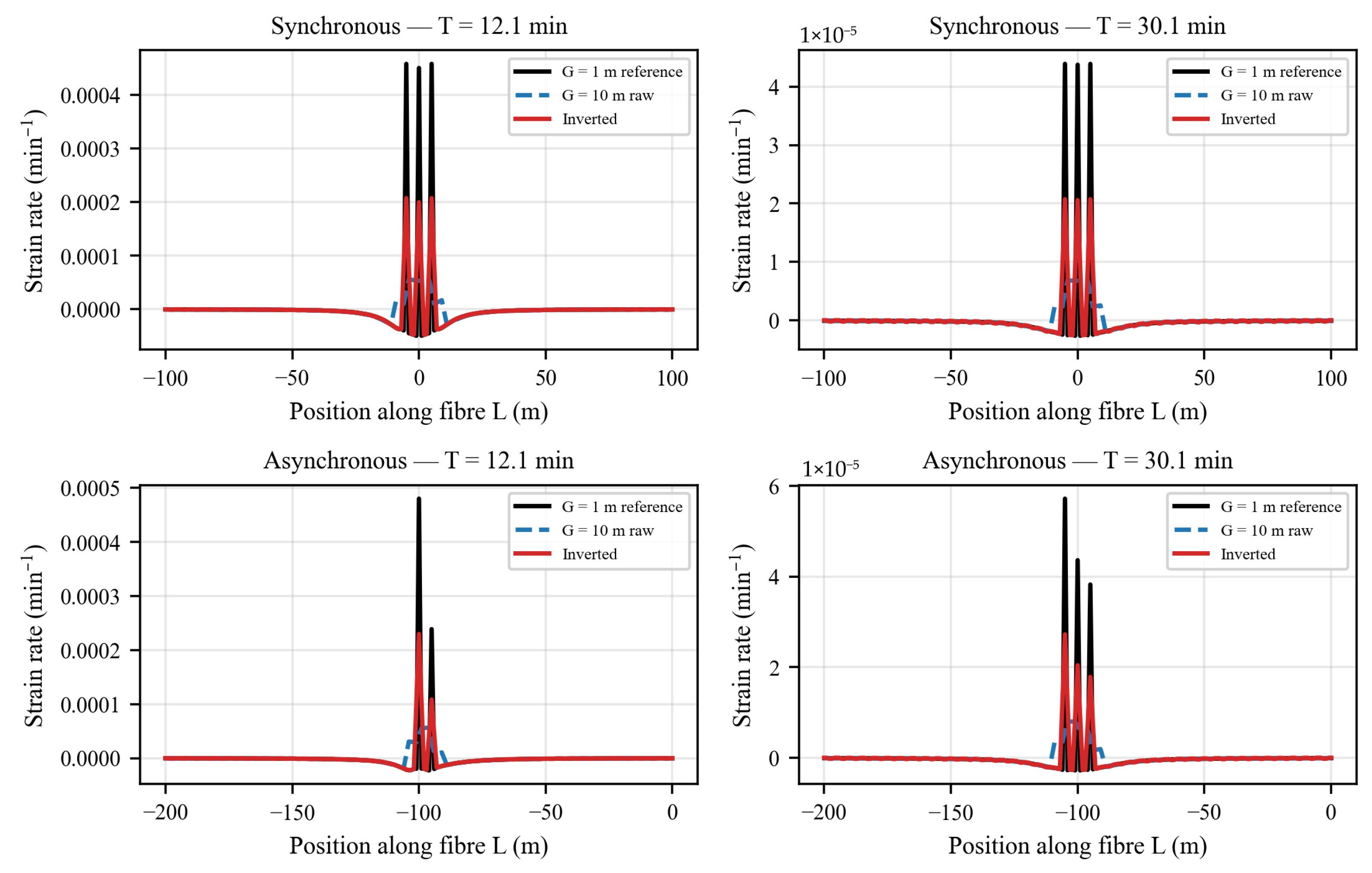
To complement the visual waterfall comparison, quantitative diagnostics are reported for the synchronous-fracture benchmark (Table 3). All RMSE, MAE, and Pearson r values listed in the table are strict metrics which are computed by comparing the inverted field directly against the high-resolution G = 1 m reference. As a separate sanity check, a self-consistency test is also performed: the inverted field is re-averaged with the original G = 10 m gauge-averaging operator and compared against the input observation (see table footnote). (i) Self-consistency of the regularized inversion method: after re-applying the gauge-averaging operator to the inverted strain-rate field, the residual relative to the original G = 10 m measurement reaches an RMSE of 9.57 × 10⁻⁹ s−1 (R2 = 1.000), confirming that the inverted solution reproduces the input observation almost perfectly. (ii) Peak-structure recovery: during the fracture-hit window (T = 12–50 min) the inverted field recovers the correct fracture count in 100% of the time slices, whereas the raw G = 10 m measurement matches the reference fracture count in only 32%. The mean peak-position localization error drops from 0.95 m (raw) to 0.50 m (inverted), which is a 47% improvement. (iii) Strict pixel-wise agreement with the G = 1 m reference: the inverted field reaches a Pearson correlation of 0.80, versus 0.29 for the raw data. Figure 12 overlays the strain-rate profiles at three representative time slices and visually confirms that the regularized inversion method resolves the three closely spaced tensile peaks merged into a single broad band in the raw G = 10 m signal. The residual amplitude gap reflects the intrinsic information loss of inverting a wide spatial-averaging kernel and represents the theoretical limit of any post-processing super-resolution scheme.
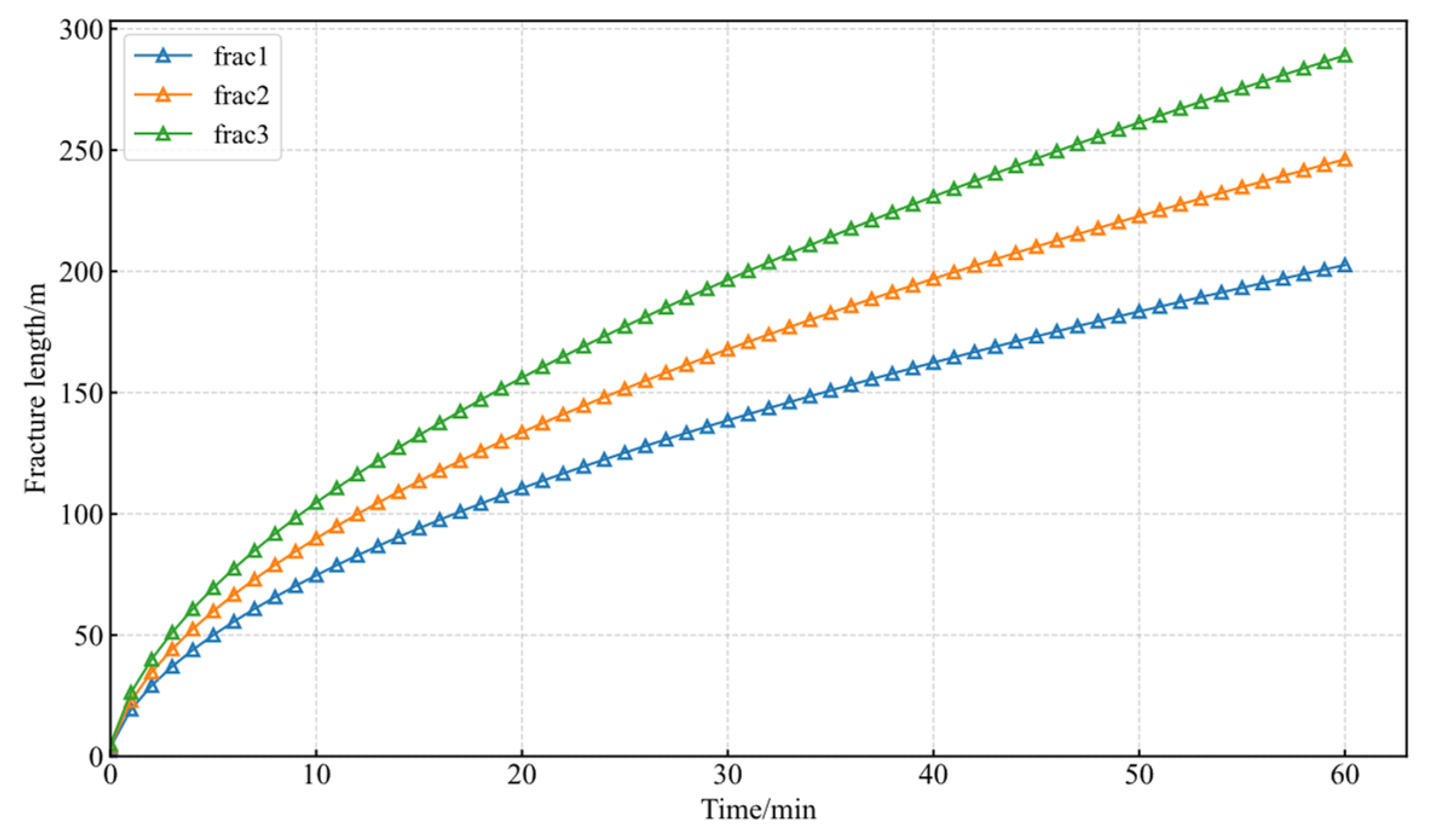
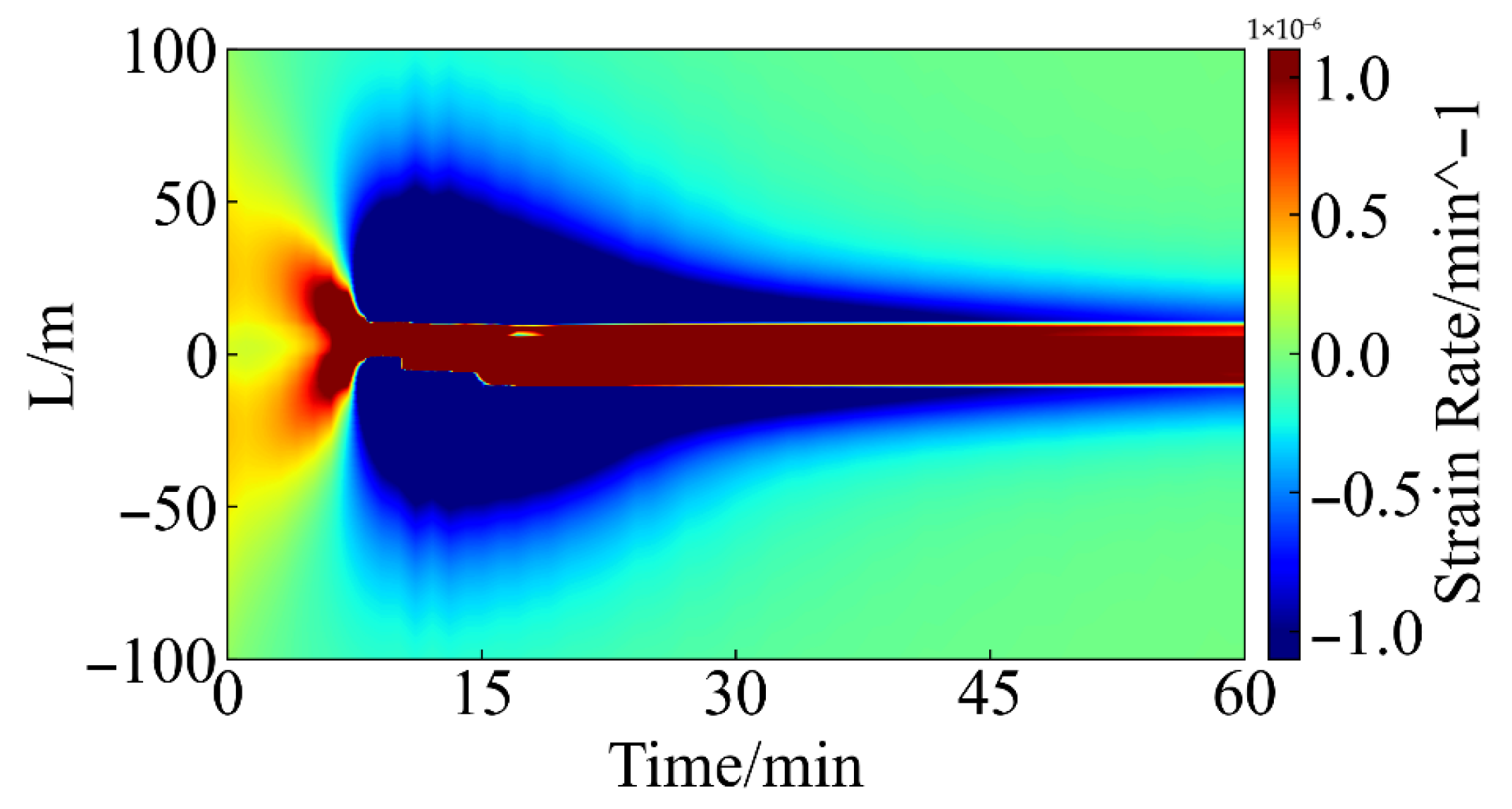
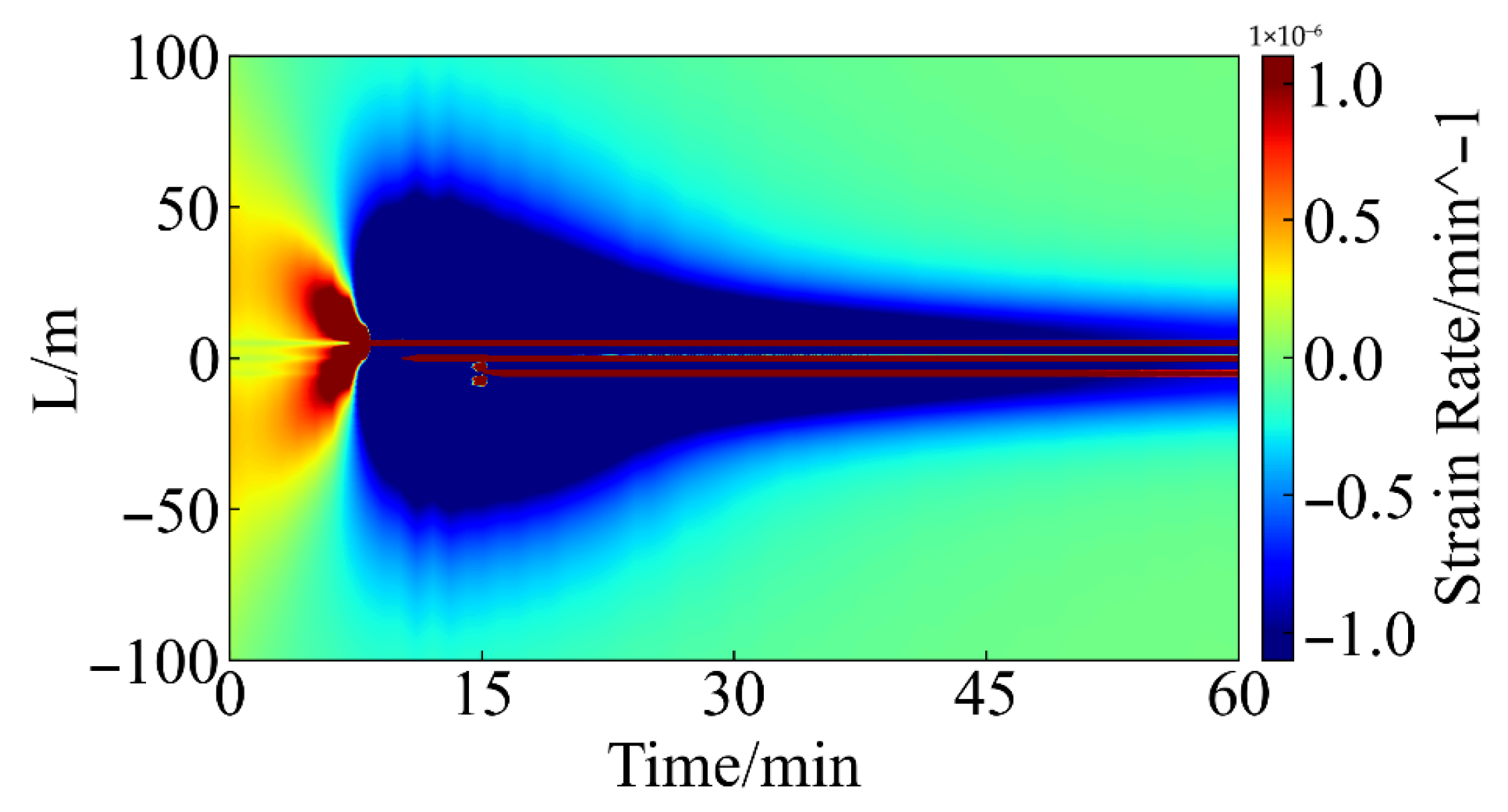
The case of asynchronous fracture propagation is further investigated. Fractures frac1, frac2, and frac3 are assigned different pumping conditions, with injection rates of 2.6, 3.2, and 3.8 m3/min, respectively, while all other propagation parameters remain identical to those listed in Table 2. The resulting fracture propagation processes are illustrated in Figure 13. Figure 14 and Figure 15 present the corresponding strain-rate waterfall plots obtained under gauge-length conditions of G = 10 m and G = 1 m, respectively.
For the G = 10 m case, the waterfall plot is able to identify the earliest-arriving fracture (frac3), which generates a tensile heart-shaped response at approximately 9 min. Subsequently, localized intensification and thickening of the tensile band are observed near 12 min and 17 min, reflecting the superposition effects induced by the successive arrival of the remaining fractures. However, owing to the pronounced spatial averaging associated with the large gauge length, the individual tensile bands corresponding to different fractures cannot be clearly separated.
Under the G = 1 m condition, the waterfall plot provides a clearer characterization of the spatial locations of individual fractures and their corresponding arrival times. It should be noted that, due to stress interactions among fractures, the fractures arriving later do not necessarily exhibit a typical “heart-shaped fracture hit” signature. Nevertheless, the spatial positions of the tensile bands and their temporal intensification patterns can still be used to identify fracture propagation and arrival processes, and they remain consistent with the true fracture growth obtained from numerical simulations. The waterfall plot obtained by applying the proposed resolution enhancement method to the G = 10 m data is shown in Figure 16. The results indicate that the enhanced-resolution waterfall plot exhibits strong agreement with the G = 1 m reference solution in terms of the major spatiotemporal features, enabling accurate recovery of the propagation and arrival characteristics of the three fractures.
In summary, both sets of comparative benchmark cases demonstrate that the proposed neighbor-well LF-DAS spatial resolution-enhancement method can effectively recover the key features of closely spaced multi-fracture propagation under large gauge-length (low native-resolution) conditions. The enhanced results exhibit strong consistency with the high-resolution reference responses, indicating that the method has considerable potential for practical identification and characterization of clustered fractures in field applications.
The same quantitative diagnostics applied to the asynchronous-fracture benchmark give RMSE = 9.29 × 10⁻⁹ s−1 and R2 = 1.000 for the self-consistency test, a peak count match rate of 95% versus 13% for the raw G = 10 m data, and a Pearson correlation of 0.81 versus 0.29 (Table 3). The asynchronous benchmark therefore reproduces all qualitative trends of the synchronous case and confirms that the advantages of the regularized inversion method are not tied to a particular fracture-propagation scenario.

3.2. Noise Sensitivity

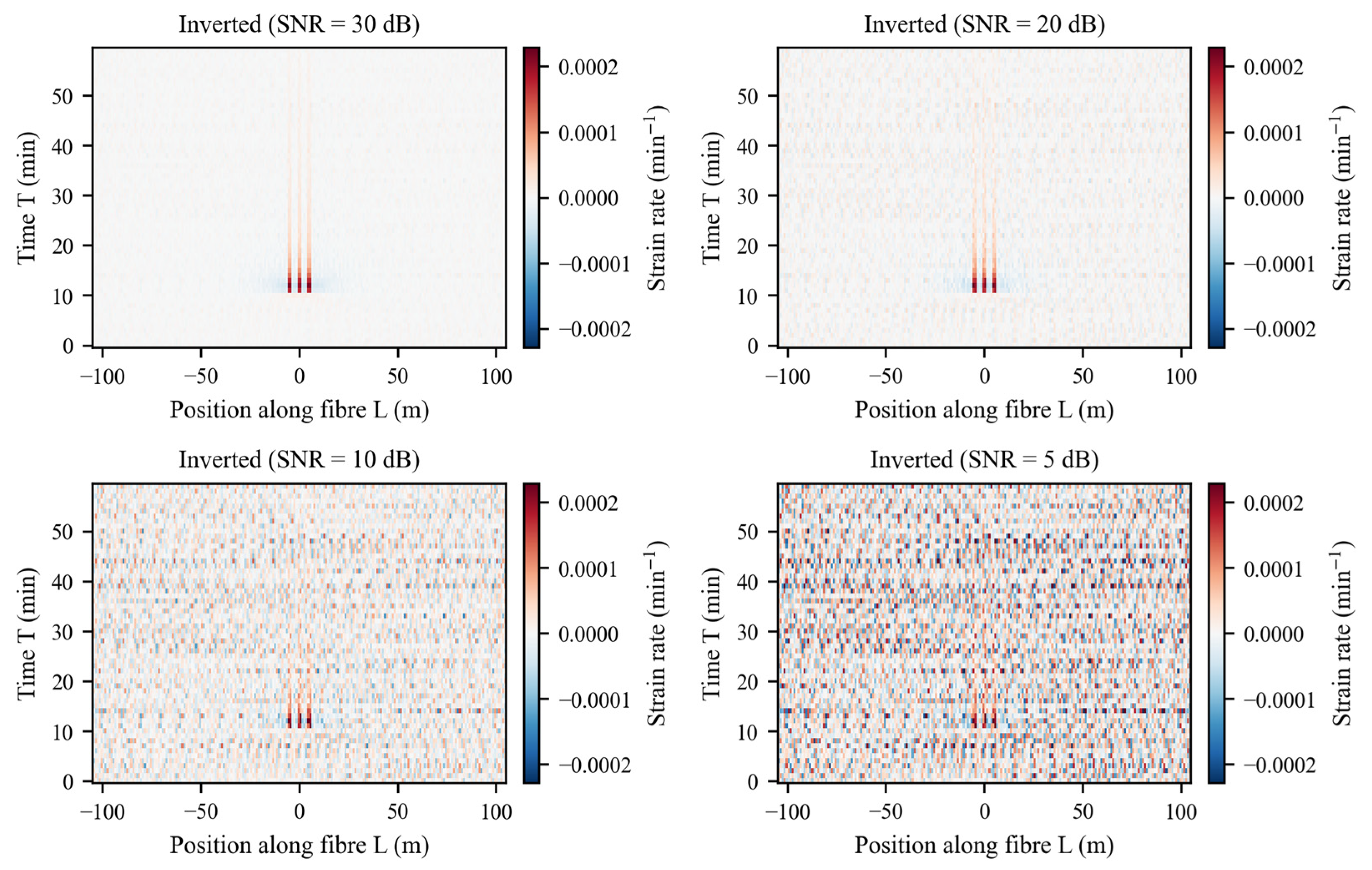
A noise-sensitivity study of the regularized inversion method was carried out by injecting zero-mean Gaussian noise on top of the synchronous-fracture G = 10 m benchmark at four SNR levels (30, 20, 10 and 5 dB). For each level, the regularized inversion method is applied with identical settings and the resulting field is compared with the high-resolution G = 1 m reference solution (Table 4, Figure 17). The data-fidelity term remains essentially saturated across the whole SNR sweep, the self-consistency R2 between the inverted solution (after re-applying the gauge averaging operator) and the noisy observation stays at 1.000 (SNR = 30 dB), 1.000 (SNR = 20 dB), 0.999 (SNR = 10 dB) and 0.999 (SNR = 5 dB), confirming that the inverted field always reproduces the noisy observation it was given. The strict pixel-wise Pearson correlation against the G = 1 m reference, however, decreases monotonically with decreasing SNR (from 0.777 at 30 dB to 0.175 at 5 dB) and the peak count match rate degrades from 71% at SNR = 30 dB to 24% at SNR = 20 dB and to 3% at SNR ≤ 10 dB. These results indicate that the regularized inversion method preserves clean-data accuracy when the acquisition SNR is above ~20 dB; when the SNR drops below 20 dB, the additive noise begins to dominate the high-frequency content of the inverted solution and an additional preprocessing step (e.g., wavelet denoising, Algorithm 1 step 6) should be applied before the inversion.

3.3. Baseline Comparison with a Wiener Filter

To put the regularized inversion method into a quantitative context, it is compared against a Wiener filter on the synchronous-fracture benchmark. The Wiener filter is a standard linear minimum-mean-square-error smoothing operator that computes each output sample as a local-variance-weighted blend of the raw sample and the local mean. It requires only a single parameter, the smoothing-window length, which is set to five samples (approximately matching the enhancement factor G/dl) for all scenarios tested here. Crucially, the Wiener filter does not incorporate any knowledge of the gauge-averaging operator and therefore represents the “no gauge-awareness” lower bound of what any linear post-processing step can deliver. Benchmarking against it isolates the specific benefit of explicitly inverting the gauge-averaging convolution.
Four scenarios are evaluated: the clean G = 10 m measurement and three additive-Gaussian-noise conditions (SNR = 20 dB, 15 dB and 10 dB). In every noisy scenario, the proposed method is applied with the optional wavelet pre-denoising step turned on, consistent with the practical recommendation of Section 3.2.
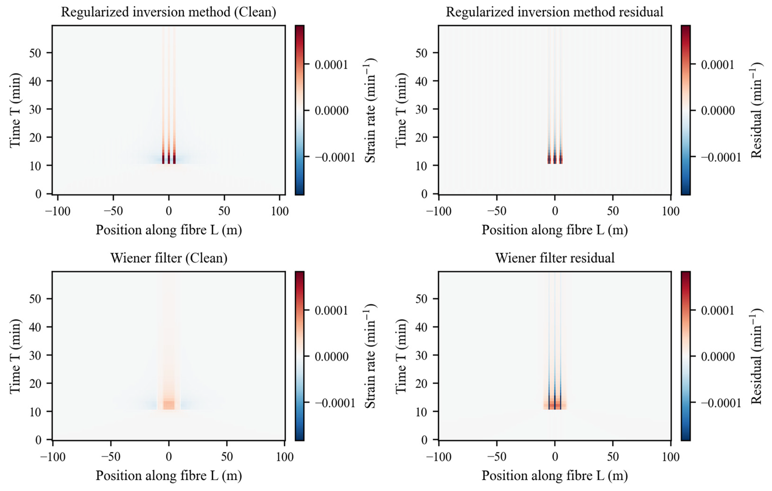
On clean data, the regularized inversion method achieves a Pearson correlation of 0.80 against the G = 1 m reference and recovers the correct number of three tensile peaks in 100% of the time slices, whereas the Wiener filter reaches only 0.30 and 68%, respectively (Figure 18, Table 5).
Under additive Gaussian noise, the regularized inversion method (with wavelet pre-denoising) retains a decisive advantage at all tested SNR levels. Its Pearson correlation degrades gracefully from 0.67 at 20 dB to 0.58 at 15 dB and 0.43 at 10 dB, while the Wiener filter’s Pearson correlation remains essentially constant at r ≈ 0.30 (specifically 0.297, 0.297, 0.295 at 20/15/10 dB), confirming that its information content about the underlying multi-fracture structure does not vary significantly with SNR and is fundamentally limited by the absence of gauge-length-operator inversion. The peak count match rate of the proposed method decreases monotonically (66% → 55% → 42%), whereas the Wiener filter’s peak count match rate shows a non-monotonic behavior (29% → 34% → 21%). This non-monotonic behavior is a consequence of the fact that, because the Wiener filter does not attempt to invert the gauge-averaging operator, its peak count agreement with the G = 1 m reference is effectively stochastic: it reflects the chance alignment of the locally smoothed profile with the true peak positions at each noise realization, rather than a principled SNR-dependent recovery of multi-fracture structure. This is why the more robust pixel-wise Pearson correlation remains flat across noise levels while the peak count match rate fluctuates.
Across the full SNR range from clean data down to 10 dB, the regularized inversion method therefore outperforms the Wiener filter by approximately 1.5–2.7× in Pearson correlation and 1.5–2.3× in peak count match rate, demonstrating that explicitly inverting the gauge-averaging operator offers a fundamental advantage over a generic linear smoothing filter, an advantage that persists under realistic field-level noise once the recommended wavelet pre-denoising step is applied.

4. Discussion

This section investigates the characteristics of neighbor-well LF-DAS strain-rate responses under different combinations of fiber-optic gauge length and sample spacing, with particular emphasis on the sensitivity of the proposed spatial resolution-enhancement method to variations in these parameters and the resulting improvement in resolving capability. To ensure controlled and consistent comparisons, the numerical cases considered herein adopt the same geometric configuration and fracture propagation settings as those used in the previous validation section. Specifically, the distance between the treatment well and the horizontal neighbor-well is set to 100 m, and three fractures are arranged parallel to the wellbore direction with an inter-fracture spacing of 5 m (Figure 7). Fracture propagation is simulated using the PKN model, and the corresponding neighbor-well fiber-optic strain responses are computed using the semi-analytical multi-fracture forward model developed in this study.
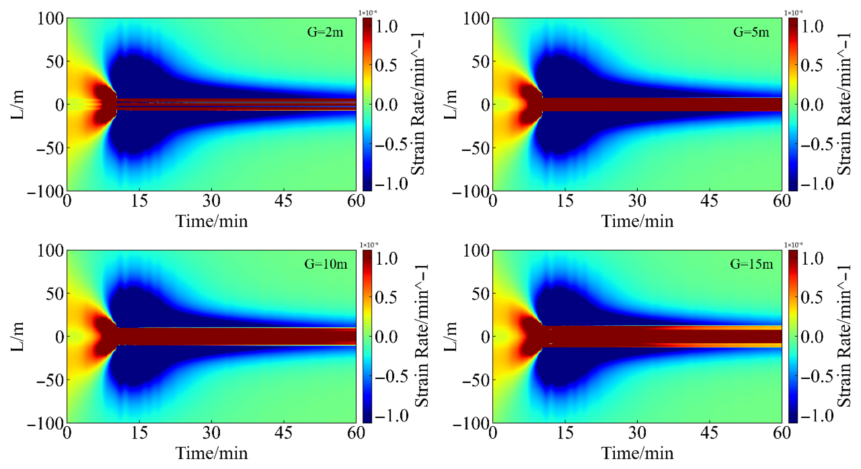
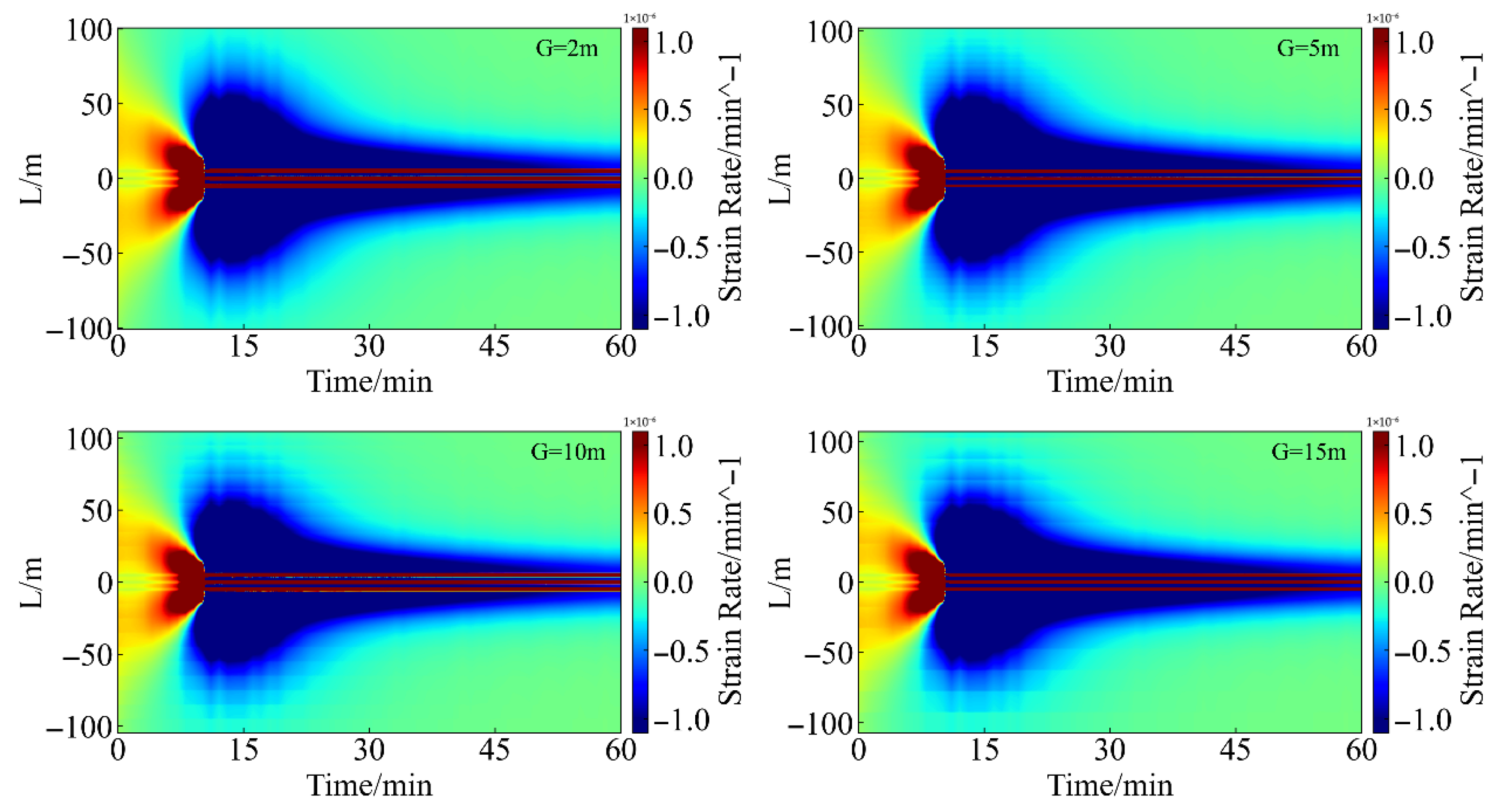
First, with the sample spacing fixed at dl = 1 m, neighbor-well fiber-optic strain-rate responses are computed for four gauge-length conditions, namely G = 2, 5, 10, and 15 m (Figure 19). The proposed resolution enhancement method is then applied to each case, yielding the corresponding enhanced strain-rate waterfall plots (Figure 20).
As shown in Figure 19, the gauge length exerts a dominant influence on the spatial resolving capability of the original neighbor-well LF-DAS data. With increasing gauge length, the spatial averaging effect inherent in the measurement process becomes progressively more pronounced. Consequently, the strain responses induced by multiple closely spaced fractures show increasing amounts of overlap, making it difficult to clearly identify the number of fractures and their independent propagation characteristics from the waterfall plots.
In contrast, the resolution-enhanced results shown in Figure 20 exhibit highly consistent spatiotemporal features across different gauge-length conditions. Despite the substantial differences in gauge length in the original measurements, the processed waterfall plots are able to recover, to a large extent, the spatial locations and propagation histories of the three fractures for all cases. Moreover, only minor discrepancies are observed among the enhanced results obtained with different gauge lengths. These observations indicate that, for a given sample spacing, the proposed resolution enhancement method demonstrates strong robustness with respect to variations in gauge length, and its effective resolving capability does not degrade significantly as the gauge length increases.
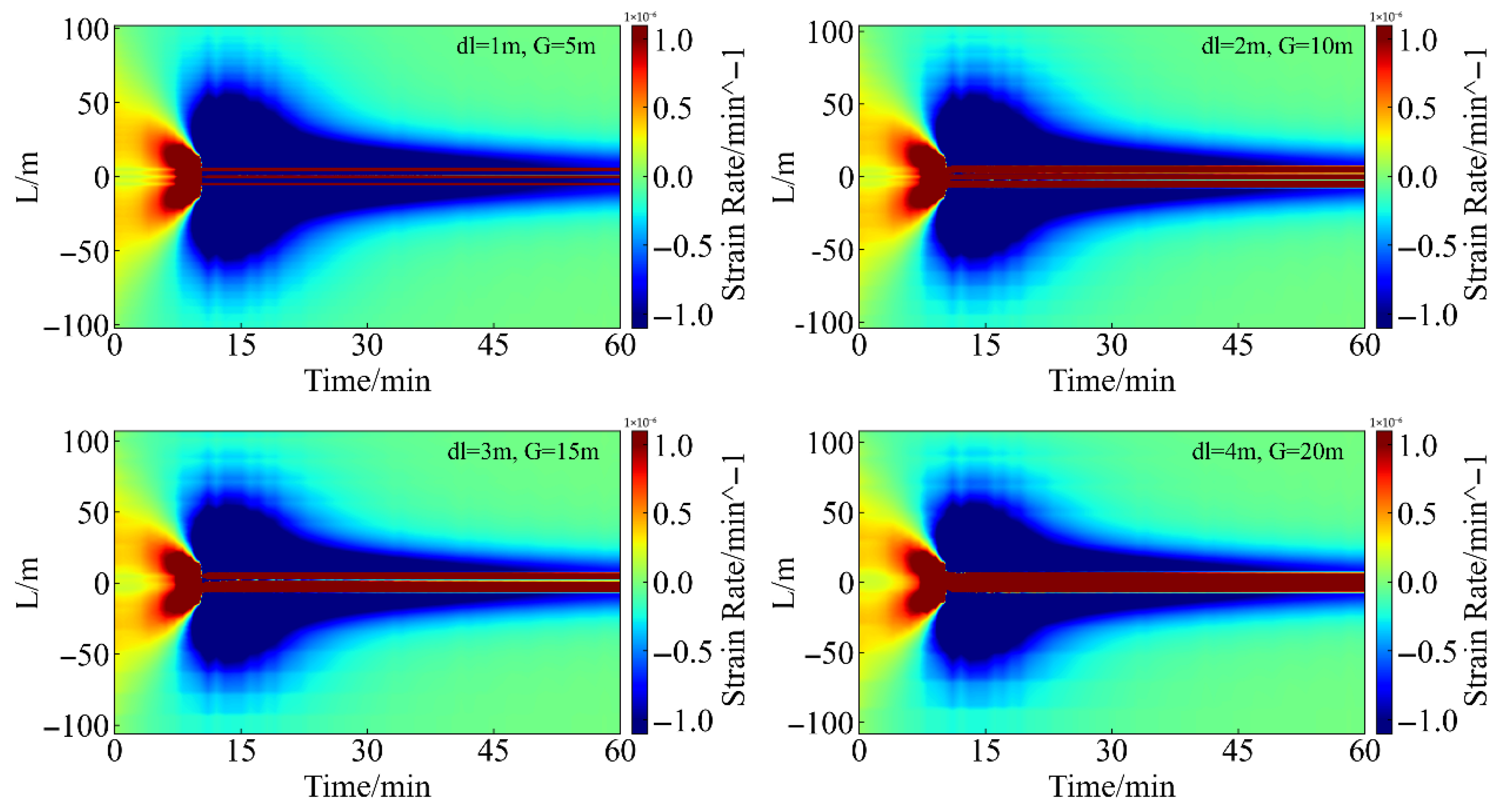
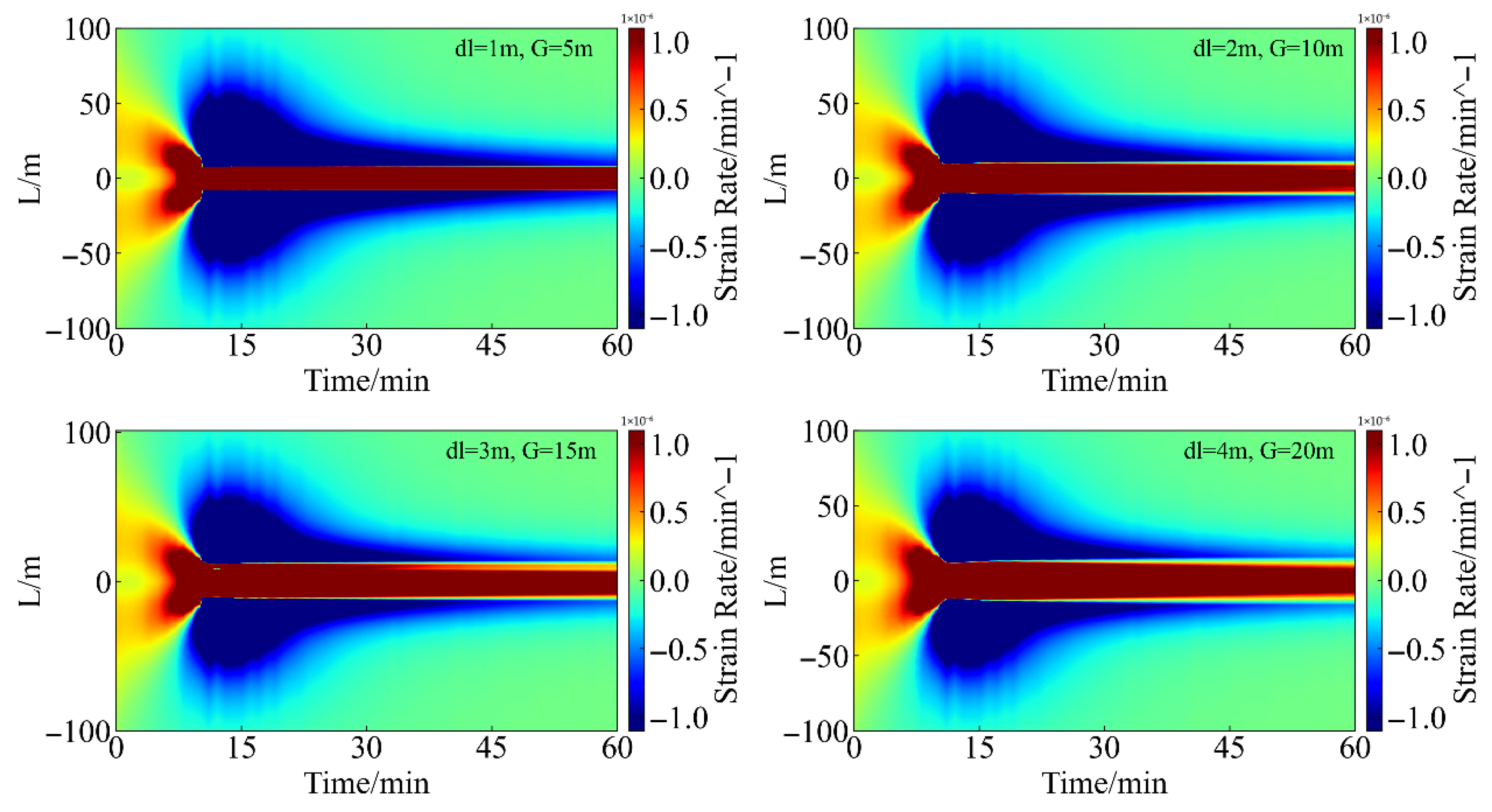
The influence of sample spacing on the effectiveness of the resolution enhancement method is further analyzed. In this subsection, the resolution enhancement factor is kept constant at G/dl = 5. Sample spacings of dl = 1, 2, 3, and 4 m are considered, with the corresponding gauge lengths set to G = 5, 10, 15, and 20 m, respectively. The neighbor-well fiber-optic strain-rate responses under these parameter combinations are shown in Figure 21, and the corresponding resolution-enhanced results are presented in Figure 22. The results indicate that, even under an identical resolution enhancement factor, the final resolving performance differs markedly for different sample spacings. As the sample spacing dl decreases, the fracture-induced tensile bands in the enhanced waterfall plots become more distinct, spatial localization errors are reduced, and the resolvability of multi-fracture propagation is significantly improved. In contrast, when the sample spacing is relatively large, the ultimate resolving capability remains constrained by the discrete nature of the measurements, even if the same resolution enhancement factor is applied.
These results indicate that the sample spacing fundamentally governs the upper limit of the achievable accuracy of the proposed resolution enhancement method. A smaller sample spacing provides a higher spatial sampling density, allowing the inverted subinterval strain-rate distribution to more closely approximate the true high-resolution response. In contrast, when the sample spacing is relatively large, insufficient spatial sampling constrains the ultimate accuracy attainable through resolution enhancement.
Overall, the above analyses demonstrate that the proposed neighbor-well LF-DAS spatial resolution-enhancement method can effectively recover the key features of closely spaced multi-fracture propagation across a wide range of gauge-length conditions, exhibiting strong robustness with respect to gauge-length variations. Meanwhile, the ultimate achievable resolution is governed by the sample spacing: a smaller sample spacing provides greater potential for resolution enhancement. This finding offers a quantitative guideline for the design of field LF-DAS monitoring parameters, indicating that, while satisfying signal-to-noise ratio requirements, a smaller sample spacing should be preferentially adopted to fully exploit the advantages of the proposed resolution enhancement method.
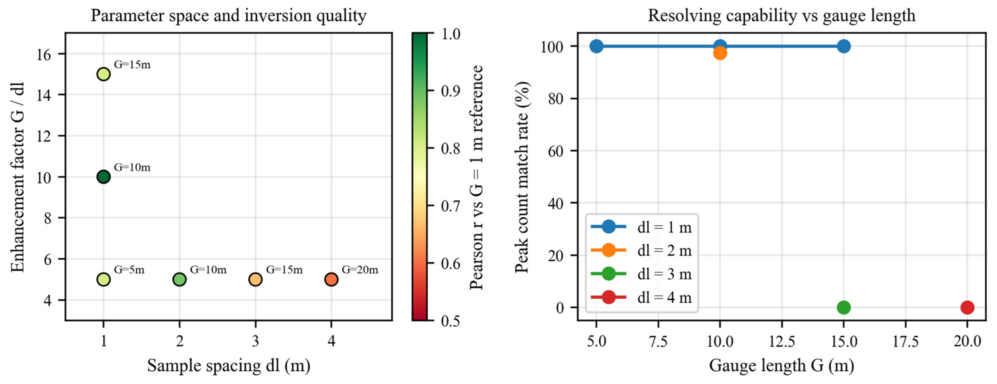
To make the role of the gauge length G and the sample spacing dl quantitative, six representative (G, dl) combinations were processed by the regularized inversion method under identical fracture geometry, formation properties and noise level (Figure 23). The highest-resolution combination (G = 2 m, dl = 1 m) is used as the reference solution (Table 6). Two complementary trends emerge:
(1)
For a fixed sample spacing of dl = 1 m, the Pearson correlation between the inverted strain-rate field and the reference stays in the 0.80–1.00 range across the three gauge lengths tested (G = 5, 10, 15 m), and the peak-count match rate is 100% in every case. This confirms that, once the sample spacing is small enough, the regularized inversion method is essentially insensitive to the choice of gauge length.
(2)
For a fixed enhancement factor of G/dl = 5, the Pearson correlation grows monotonically as dl decreases (Pearson r ≈ 1 − 0.1 dl). The peak count match rate jumps from 0% at dl = 4 m (G = 20 m) to 100% at dl = 1 m (G = 5 m). The best and worst combinations differ by a factor of 1.7, with the gain almost entirely attributable to the smaller dl.
These observations support the conclusion that the ultimate resolution of the regularized inversion method is governed by the sample spacing dl, while the gauge length G mainly determines how much spatial averaging the inversion must compensate for. Based on the above analysis, two practical recommendations for field LF-DAS acquisition design can be formulated:
(1)
Prioritize dl over G. Within the SNR budget of the interrogator, choose the smallest possible dl. Increasing G to maintain SNR is acceptable because the spatial averaging induced by G can be largely undone by the regularized inversion method.
(2)
Keep G as an integer multiple of dl so that the overlap matrix A remains sparse and well-conditioned, and aim for an enhancement factor G/dl in the range 5–10. The typical “sweet spot” for clustered-fracture monitoring is dl ≈ 1 m and G/dl in this range, corresponding to an effective resolution of about 1 m at no additional acquisition cost.

5. Field Application

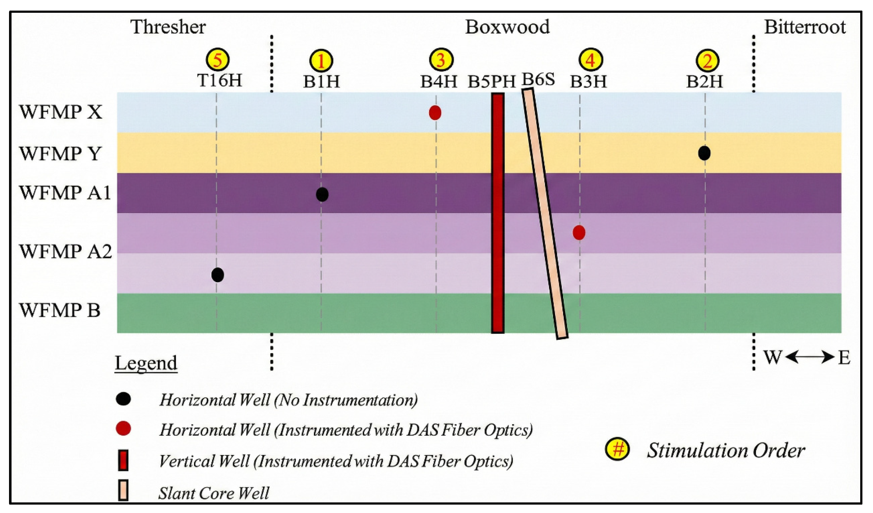
To evaluate the proposed method under realistic field conditions, it is applied to LF-DAS data from the second phase of the Hydraulic Fracturing Test Site (HFTS-2) in the Permian Basin, United States [21,22,42,43,44,45,46,47,48]. The dataset consists of neighbor-well strain-rate data recorded in well B3H during the hydraulic fracturing of stages 22 and 23 in well B1H. The fiber in B3H was deployed behind casing with a gauge length of G = 7.147 m and a sample spacing of dl = 1.021 m, yielding an enhancement factor G/dl ≈ 7. Prior to the regularized inversion, the raw strain-rate field is preprocessed through (i) a band-pass filter to retain low-frequency content relevant to hydraulic-fracture propagation, (ii) a common-mode removal step to suppress tube-wave and interrogator-level noise, (iii) a median time-domain detrending step to remove slow drift, and (iv) a channel-level quality control step that flags and excludes dead or saturated channels. The same data-conditioning pipeline is applied to both stages. The spatial configuration of the wells involved in the HFTS-2 experiment is illustrated in Figure 24.
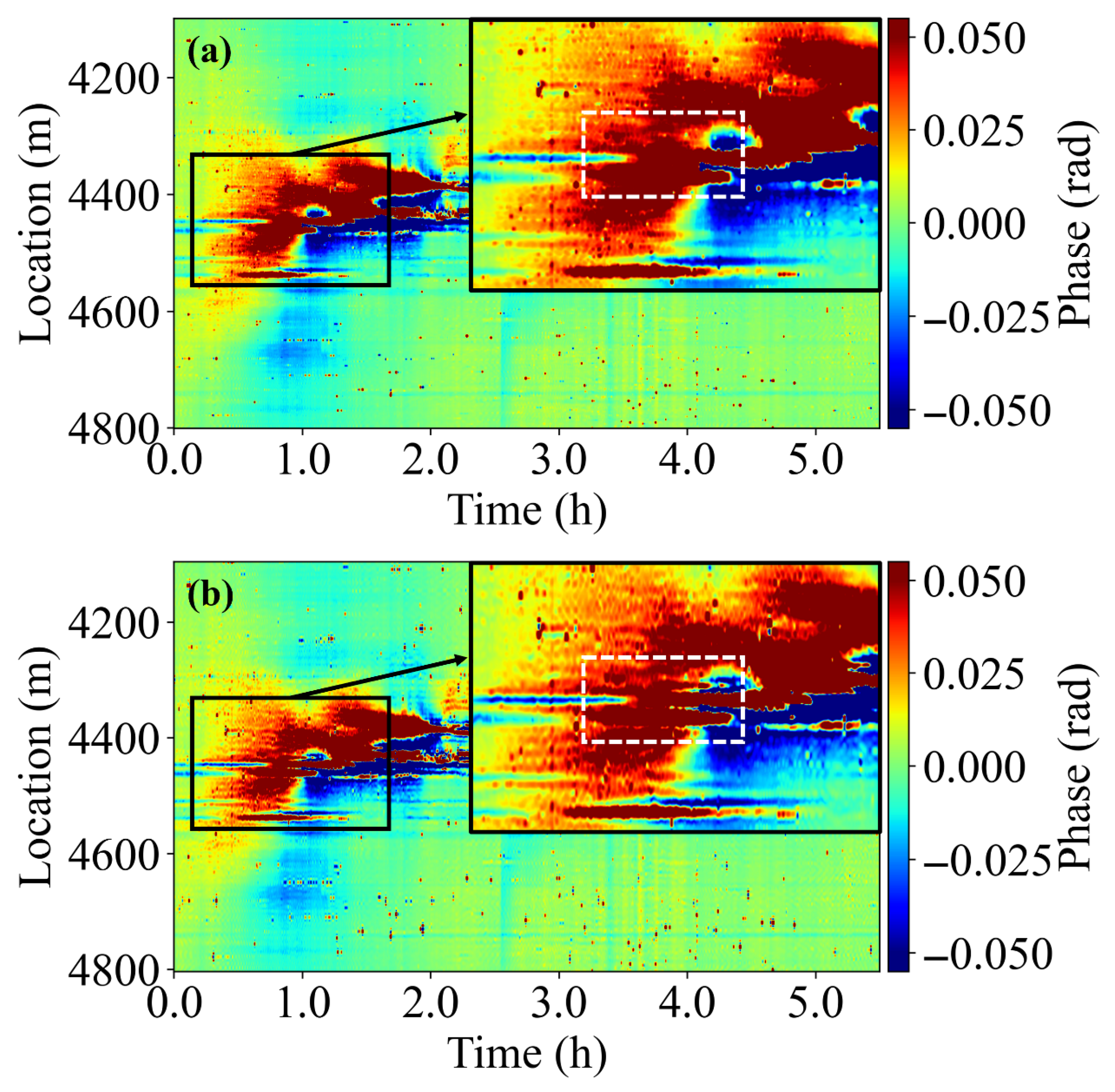
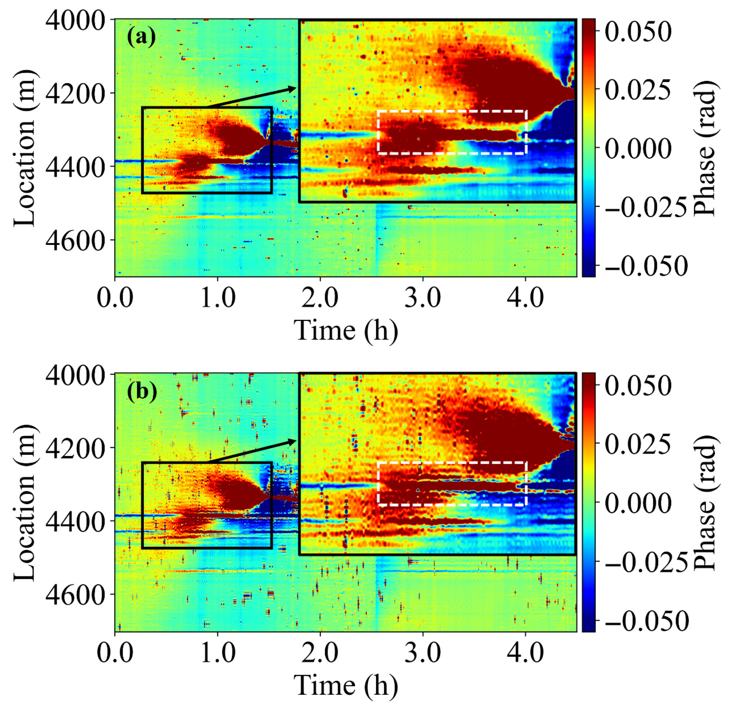
Figure 25 and Figure 26 present comparisons between the original LF-DAS measurements and the corresponding resolution-enhanced strain-rate waterfall plots for stages 22 and 23 of well B1H, respectively. As observed, the original data exhibit relatively blurred and continuous spatial responses, with pronounced overlap among fracture-induced tensile bands, making it difficult to clearly identify the number of fractures and their independent propagation processes. In contrast, after applying the proposed resolution enhancement method, the waterfall plots reveal substantially richer and clearer spatial details. The strain-rate responses associated with multiple closely spaced fractures can be more distinctly resolved in both space and time, and the fracture propagation and arrival processes become more readily identifiable.
Notably, the densely distributed multi-fracture features identified after resolution enhancement show qualitative consistency with the clustered fracture patterns revealed by post-fracturing core observations from the HFTS-2 experiment. This agreement provides further field-based evidence supporting the prevalence of clustered fractures in hydraulically fractured unconventional reservoirs. Moreover, it demonstrates that the proposed method is capable of effectively extracting fracture-geometry information from neighbor-well fiber-optic data under practical conditions characterized by high noise levels and strong spatial averaging effects.
In summary, the proposed neighbor-well LF-DAS spatial resolution-enhancement method demonstrates good applicability and stability when applied to the HFTS-2 field dataset. The method is capable of substantially improving the spatial resolving capability of the original fiber-optic measurements, thereby providing an effective and practically applicable tool for refined interpretation of hydraulic fracture geometry and identification of clustered fracture patterns in field-scale hydraulic fracturing operations.
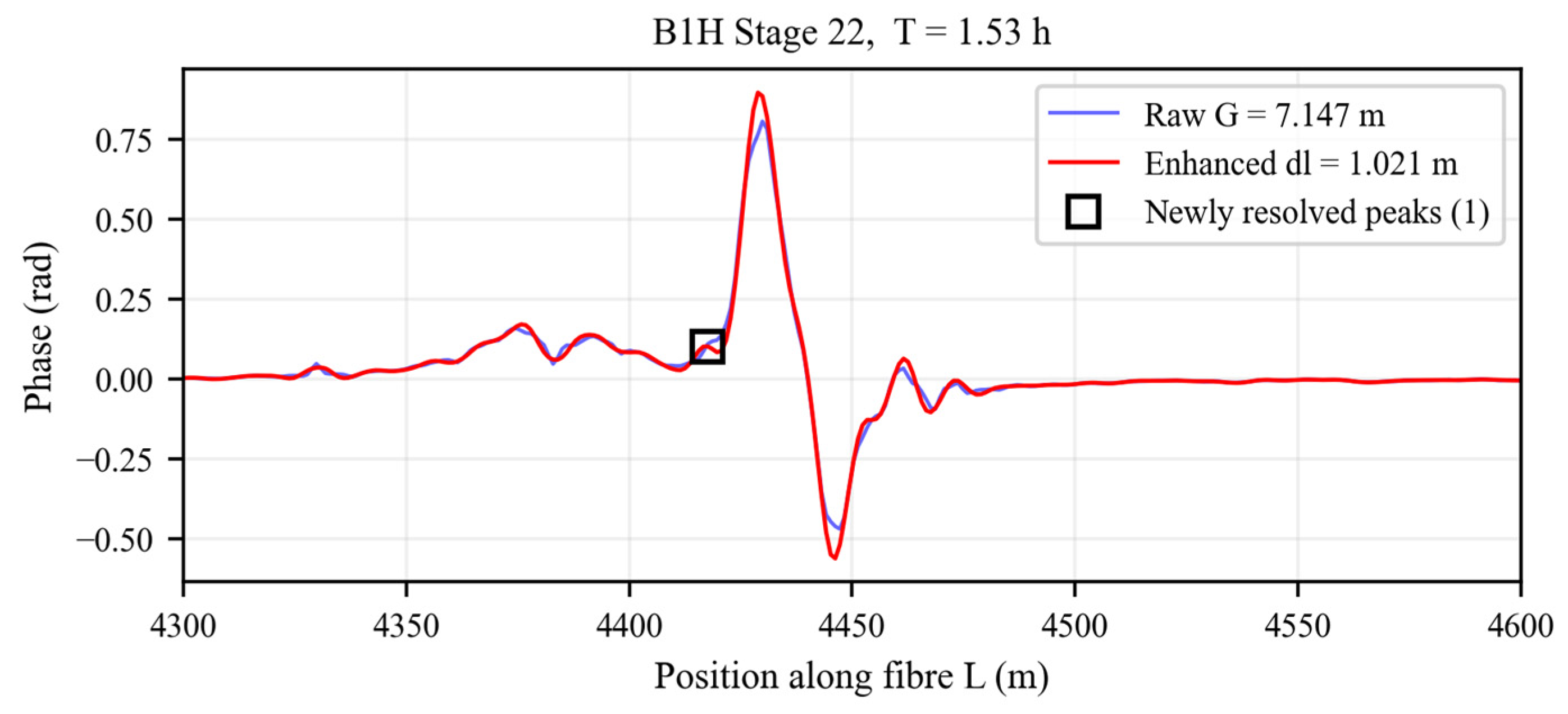
To complement the visual waterfall comparison, resolution-enhanced strain-rate profiles are examined at representative fracture-hit time slices to assess whether the inversion reveals fracture features that are hidden in the original measurement.
For Stage 22 (Figure 27, T = 1.53 h), the raw G = 7.147 m profile shows a smooth, monotonic rise from L ≈ 4400 m to the main tensile peak at L ≈ 4429 m. After enhancement, a distinct new tensile peak emerges at L ≈ 4418 m on this formerly featureless ascending flank, suggesting the presence of an additional fracture that was completely masked by the gauge-length spatial averaging. This peak is absent in the raw profile and cannot be attributed to noise amplification, as the surrounding baseline remains clean.
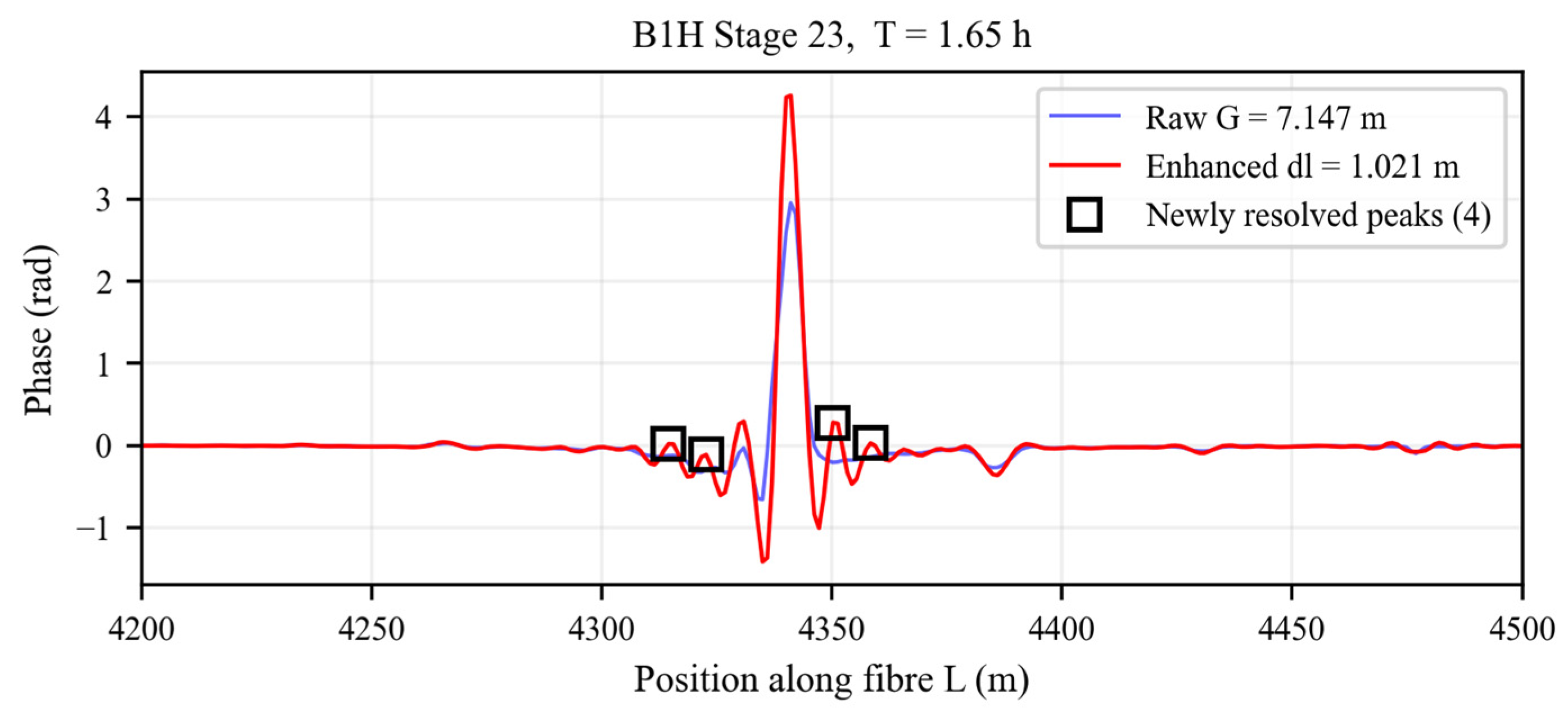
For Stage 23 (Figure 28, T = 1.65 h), the effect is more pronounced. The raw measurement shows only a single broad tensile band centered near L ≈ 4341 m, whereas the enhanced profile resolves four additional peaks: two on the ascending flank (L ≈ 4315 m and L ≈ 4323 m) and two on the descending flank (L ≈ 4350 m and L ≈ 4358 m). The original single-band response is thus decomposed into a cluster of distinct tensile features, indicating a higher local fracture density than can be inferred from the raw data alone.
It should be noted that the G/dl ≈ 7 enhancement factor represents a theoretical upper bound on the resolution improvement, not a guaranteed multiplicative factor on the number of observed features. The features actually resolved in a field measurement are constrained by the physical inter-fracture spacing of the true fracture network. The newly identified features are qualitatively consistent with the densely clustered fracture patterns documented in the HFTS-2 slant-core observations by Gale et al. [22] and Raterman et al. [20]. Microseismic and production data for B1H stages 22 and 23 are not publicly available; cross-validation against those modalities will be performed in future work.
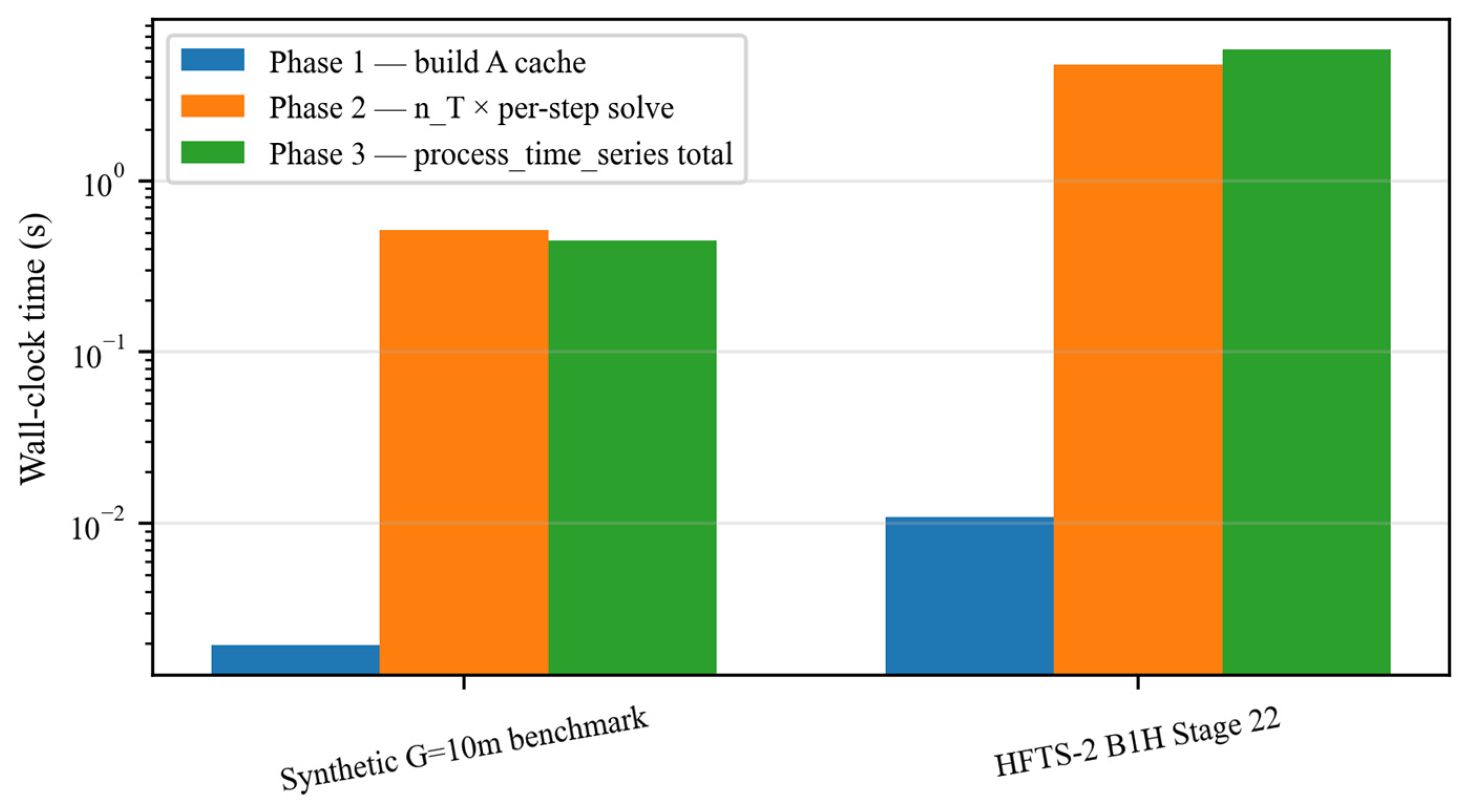
The regularized inversion method is computationally inexpensive enough to be deployed in a real-time monitoring loop. On a standard Intel workstation, the cost decomposes into three phases: (1) building the overlap matrix A takes only 2.13 ms for the synthetic benchmark and 21.84 ms for the HFTS-2 B1H stage 22 dataset; this cost is incurred only once per acquisition geometry. (2) Inverting one time step through the cached operators takes 7.59 ms (synthetic) and 5.23 ms (field). (3) End-to-end processing of the entire stage runs in 0.44 s (synthetic) and 17.64 s (field), corresponding to throughputs of 137 and 112 time steps per second, respectively. Since the matrix A only depends on the acquisition geometry (gauge length and sample spacing) and is independent of the interrogator manufacturer, the proposed framework is directly transferable to any LF-DAS deployment for which these parameters are known. The runtime budget is comfortably within the requirements of a real-time monitoring loop and the cost scales linearly with the number of channels and time samples (Figure 29, Table 7).

6. Conclusions

In this study, a spatial resolution-enhancement method for neighbor-well LF-DAS data in hydraulic fracturing is developed based on the concept of a regularized inversion method, in combination with a recursive prior and a second-order difference L-curve optimization strategy. The proposed approach effectively upgrades the usable spatial resolution of fiber-optic measurements from the gauge-length scale to the sensor-spacing scale. Meanwhile, an efficient semi-analytical forward model for neighbor-well fiber-optic strain responses under multi-fracture propagation is constructed based on the Boussinesq solution, together with coordinate transformation and linear superposition principles. This forward model is further employed to verify the accuracy and applicability of the proposed resolution enhancement method. The main conclusions of this study are summarized as follows:
  • During the monitoring of vertical hydraulic fracture propagation using fiber-optic measurements in a horizontal neighbor-well, the neighbor-well LF-DAS data exhibit a characteristic tensile “heart-shaped” strain-rate pattern as the fracture front progressively approaches and intersects the monitoring well. This signature serves as an effective indicator of fracture hit. Following fracture hit, a stable tensile band is formed at the corresponding spatial location along the fiber. Under coupled multi-fracture propagation conditions, however, the spatial averaging effect introduced by the fiber-optic gauge length significantly degrades the resolving capability of the original LF-DAS data, making it difficult to distinguish the independent propagation behavior of individual fractures and thereby obscuring fracture numbers and geometric information;
  • The efficient multi-fracture neighbor-well fiber-optic strain forward model developed based on the Boussinesq half-space solution does not require spatial discretization of the computational domain. By employing coordinate transformation and stress (displacement) superposition, the fiber-optic strain responses induced by multiple fractures can be computed directly. As a result, the model maintains high computational efficiency even under conditions involving closely spaced fractures and a large number of fractures, effectively avoiding the rapid increase in computational cost associated with local mesh refinement in conventional grid-based methods;
  • Numerical validation and parameter-sensitivity analyses of multi-fracture neighbor-well fiber-optic strain responses demonstrate that the proposed LF-DAS resolution enhancement method can stably and accurately invert the spatial characteristics of closely spaced multi-fracture propagation. The resolution enhancement factor is governed by the ratio between the gauge length and the sample spacing (G/dl), whereas the ultimate achievable resolution is primarily controlled by the sample spacing. Specifically, a smaller sample spacing yields a higher upper limit of inversion accuracy attainable by the resolution enhancement method.
  • The results demonstrate that the regularized-inversion-based resolution enhancement method for neighbor-well LF-DAS data exhibits strong applicability in both numerical benchmarks and field datasets characterized by high noise levels. The method significantly improves the spatial resolving capability of neighbor-well fiber-optic measurements, thereby enhancing the accuracy of interpreting fracture numbers and propagation processes. It provides a reliable theoretical foundation and practical technical support for refined interpretation of neighbor-well fiber-optic data under complex fracture configurations, such as clustered fracture systems.
  • From an engineering perspective, the proposed method is a pure post-processing workflow that requires no modification to the fiber cable, interrogator, or acquisition procedure. With a per-time-step computational cost of only 5–8 ms, it can be readily integrated into real-time LF-DAS monitoring loops for rapid fracture-diagnostic interpretation.

Author Contributions

Writing—original draft preparation, Y.M.; writing—review and editing, Y.M., M.C., W.S., J.L., S.W. and Y.H.; formal analysis, Y.M.; investigation, Y.M.; methodology, Y.M.; validation, Y.M.; visualization, Y.M.; supervision, M.C. and W.S. All authors have read and agreed to the published version of the manuscript.

Funding

This research was funded by the National Natural Science Foundation of China (NSFC) under the Key Program “Key mechanical issues in improving hydraulic fracturing efficiency of ultra-deep highly deviated wells” (Grant NO. 52334001).

Data Availability Statement

The numerical data and processing scripts supporting the findings of this study are available from the corresponding author upon reasonable request.

Conflicts of Interest

Authors Jiaxin Li, Su Wang were employed by the company CNPC Engineering Technology R&D Company Limited. The remaining authors declare that the research was conducted in the absence of any commercial or financial relationships that could be construed as a potential conflict of interest. The company had no role in the design of the study; in the collection, analyses, or interpretation of data; in the writing of the manuscript, or in the decision to publish the results.

References

  1. Wang, S.; Chen, M.; Lv, J.; Zhang, K.; Hao, Y.; Yao, B. Study on the Evolution Characteristics of Fiber-Optic Strain Induced by the Propagation of Bedding Fractures in Hydraulic Fracturing. Pet. Sci. 2024, 21, 4219–4229. [Google Scholar] [CrossRef] [Scilit]
  2. Ju, Y.; Song, J.; Wan, C.; Liu, P.; Tian, Y. Quantitative Visualization of 3D Stress Field Evolution during Hydraulic Fracturing in Reservoir Rocks Using 3D-Printed Models and Digital Photoelasticity Techniques. Theor. Appl. Fract. Mech. 2025, 139, 105071. [Google Scholar] [CrossRef] [Scilit]
  3. Liu, X.; Jin, Y.; Lin, B.; Zhang, Q.; Wei, S. An Integrated 3D Fracture Network Reconstruction Method Based on Microseismic Events. J. Nat. Gas Sci. Eng. 2021, 95, 104182. [Google Scholar] [CrossRef] [Scilit]
  4. Hou, B.; Zhang, Q.; Liu, X.; Pang, H.; Zeng, Y. Integration Analysis of 3D Fractures Network Reconstruction and Frac Hits Response in Shale Wells. Energy 2022, 260, 124906. [Google Scholar] [CrossRef] [Scilit]
  5. Yin, P.-F.; Yang, S.-Q.; Gao, F.; Tian, W.-L.; Zeng, W. Numerical Investigation on Hydraulic Fracture Propagation and Multi-Perforation Fracturing for Horizontal Well in Longmaxi Shale Reservoir. Theor. Appl. Fract. Mech. 2023, 125, 103921. [Google Scholar] [CrossRef] [Scilit]
  6. Wang, S.; Chen, M.; Chang, Z.; Zhang, Q.; Lv, J.; Cui, Z.; Hou, B. Experimental Study on Indoor Multi-Cluster Fracturing Based on Distributed Fibre-Optical Monitoring; OnePetro: The Woodlands, TX, USA, 2023. [Google Scholar]
  7. Kumar, A.; Sharma, M.M. Diagnosing Hydraulic Fracture Geometry, Complexity, and Fracture Wellbore Connectivity Using Chemical Tracer Flowback. Energies 2020, 13, 5644. [Google Scholar] [CrossRef] [Scilit]
  8. Mahmoud, A.; Gowida, A.; Aljawad, M.S.; Al-Ramadan, M.; Ibrahim, A.F. Advancement of Hydraulic Fracture Diagnostics in Unconventional Formations. Geofluids 2021, 2021, 4223858. [Google Scholar] [CrossRef] [Scilit]
  9. Sui, W.; Wen, C.; Sun, W.; Li, J.; Guo, H.; Yang, Y.; Song, J. Joint Application of Distributed Optical Fiber Sensing Technologies for Hydraulic Fracturing Monitoring. Nat. Gas Ind. 2023, 43, 87–103. [Google Scholar] [CrossRef]
  10. Wang, Y.; Wu, Z.; Wang, F. Research Progress of Applying Distributed Fiber Optic Measurement Technology in Hydraulic Fracturing and Production Monitoring. Energies 2022, 15, 7519. [Google Scholar] [CrossRef] [Scilit]
  11. Zhou, T.; Zhang, K.; Huang, Z.; Wang, H.; Huang, X.; Hu, J.; Ku, H. A DAS-Based Approach for Predicting Liquid Flow Velocity in Pipelines. Photonics 2026, 13, 225. [Google Scholar] [CrossRef] [Scilit]
  12. Zhang, K.; Ku, H.; Wang, S.; Zhang, M.; He, X.; Lu, H. Distributed Acoustic Sensing: A Promising Tool for Finger-Band Anomaly Detection. Photonics 2024, 11, 896. [Google Scholar] [CrossRef] [Scilit]
  13. Jin, G.; Roy, B. Hydraulic-Fracture Geometry Characterization Using Low-Frequency DAS Signal. Lead. Edge 2017, 36, 975–980. [Google Scholar] [CrossRef] [Scilit]
  14. Sang, Y.; Sui, W.; Zeng, B.; Song, Y.; Huang, H.; Guo, H.; Yang, Y.; Song, J.; Du, G. Far-Field Strain Analysis for Fiber-Optic Monitoring of Hydraulic Fracturing in a Deep Naturally Fractured Shale Reservoir. Nat. Gas Ind. 2024, 44, 56–67. [Google Scholar] [CrossRef]
  15. Liu, Y.; Wu, K.; Jin, G.; Moridis, G. Rock Deformation and Strain-Rate Characterization during Hydraulic Fracturing Treatments: Insights for Interpretation of Low-Frequency Distributed Acoustic-Sensing Signals. SPE J. 2020, 25, 2251–2264. [Google Scholar] [CrossRef] [Scilit]
  16. Liu, Y.; Wu, K.; Jin, G.; Moridis, G.; Kerr, E.; Scofield, R.; Johnson, A. Fracture-Hit Detection Using LF-DAS Signals Measured during Multifracture Propagation in Unconventional Reservoirs. SPE Reserv. Eval. Eng. 2021, 24, 523–535. [Google Scholar] [CrossRef] [Scilit]
  17. Hao, Y.; Chen, M.; Wang, S. Research on the Mechanism of LF-DAS Fiber-Optic Strain Rate Evolution and Automatic Interpretation Method for Multivariate Monitoring Wells. Eng. Fract. Mech. 2025, 322, 111178. [Google Scholar] [CrossRef] [Scilit]
  18. Ugueto, G.; Wu, K.; Jin, G.; Zhang, Z.; Haffener, J.; Mojtaba, S.; Ratcliff, D.; Bohn, R.; Chavarria, A.; Wu, Y.; et al. A Catalogue of Fiber Optics Strain-Rate Fracture Driven Interactions. In Proceedings of the SPE Hydraulic Fracturing Technology Conference and Exhibition, The Woodlands, TX, USA, 31 January–2 February 2023; OnePetro: The Woodlands, TX, USA, 2023; p. D021S003R001. [Google Scholar]
  19. Gale, J.F.W.; Elliott, S.J.; Laubach, S.E. Hydraulic Fractures in Core from Stimulated Reservoirs: Core Fracture Description of HFTS Slant Core, Midland Basin, West Texas. In Proceedings of the 6th Unconventional Resources Technology Conference, Houston, TA, USA, 23–25 July 2018. [Google Scholar] [CrossRef] [Scilit]
  20. Raterman, K.T.; Farrell, H.E.; Mora, O.S.; Janssen, A.L.; Gomez, G.A.; Busetti, S.; McEwen, J.; Friehauf, K.; Rutherford, J.; Reid, R.; et al. Sampling a Stimulated Rock Volume: An Eagle Ford Example. SPE Reserv. Eval. Eng. 2018, 21, 927–941. [Google Scholar] [CrossRef] [Scilit]
  21. Ciezobka, J. Overview of Hydraulic Fracturing Test Site 2 in the Permian Delaware Basin (HFTS-2). In Proceedings of the 9th Unconventional Resources Technology Conference; American Association of Petroleum Geologists: Houston, TX, USA, 2021. [Google Scholar]
  22. Gale, J.F.W.; Elliott, S.J.; Rysak, B.G.; Ginn, C.L.; Zhang, N.; Myers, R.D.; Laubach, S.E. Fracture Description of the HFTS-2 Slant Core, Delaware Basin, West Texas; OnePetro: The Woodlands, TX, USA, 2021. [Google Scholar]
  23. Hartog, A.H. An Introduction to Distributed Optical Fibre Sensors; CRC Press: Boca Raton, FL, USA, 2017; ISBN 978-1-315-11901-4. [Google Scholar]
  24. Bahrampour, A.R.; Maasoumi, F. Resolution Enhancement in Long Pulse OTDR for Application in Structural Health Monitoring. Opt. Fiber Technol. 2010, 16, 240–249. [Google Scholar] [CrossRef] [Scilit]
  25. Liu, Y.; Jin, G.; Wu, K.; Moridis, G. Hydraulic-Fracture-Width Inversion Using Low-Frequency Distributed-Acoustic-Sensing Strain Data—Part I: Algorithm and Sensitivity Analysis. SPE J. 2021, 26, 359–371. [Google Scholar] [CrossRef] [Scilit]
  26. Liu, Y.; Jin, G.; Wu, K.; Moridis, G. Hydraulic-Fracture-Width Inversion Using Low-Frequency Distributed-Acoustic-Sensing Strain Data Part II: Extension for Multifracture and Field Application. SPE J. 2021, 26, 2703–2715. [Google Scholar] [CrossRef] [Scilit]
  27. Tan, Y.; Wang, S.; Rijken, M.C.M.; Hughes, K.; Ning, I.L.C.; Zhang, Z.; Fang, Z. Geomechanical Template for Distributed Acoustic Sensing Strain Patterns during Hydraulic Fracturing. SPE J. 2021, 26, 627–638. [Google Scholar] [CrossRef] [Scilit]
  28. Ramos Gurjao, K.G.; Gildin, E.; Gibson, R.; Everett, M. Investigation of Strain Fields Generated by Hydraulic Fracturing with Analytical and Numerical Modeling of Fiber Optic Response. SPE Reserv. Eval. Eng. 2022, 25, 367–379. [Google Scholar] [CrossRef] [Scilit]
  29. Srinivasan, A.; Liu, Y.; Wu, K.; Jin, G.; Moridis, G.J. Geomechanical Modeling of Fracture-Induced Vertical Strain Measured by Distributed Fiber Optic Strain Sensing. SPE Prod. Oper. 2022, 38, 537–551. [Google Scholar] [CrossRef] [Scilit]
  30. Leggett, S.; Chen, M. Evaluation of a Rapid Diagnostic Tool to Estimate Geometry Evolution of Multiple Simultaneously Propagating Fractures from Cross-Well Fiber Optic Strain Measurements. SPE J. 2024, 29, 5991–6003. [Google Scholar] [CrossRef] [Scilit]
  31. Tu, Z.; Hu, X.; Bai, J.; Zhang, T.; Lai, W.; Zhou, F. Characterize Fracture Geometry and Propagation with Low Frequency Distributed Acoustic Sensing Strain Data. Eng. Fract. Mech. 2024, 298, 109947. [Google Scholar] [CrossRef] [Scilit]
  32. Chen, J.; Leung, J.Y.; van der Baan, M. Characterization of Low-Frequency Distributed Acoustic Sensing Signals in Hydraulic Fracturing Stimulation—A Coupled Flow-Geomechanical Simulation Approach. Geomech. Energy Environ. 2024, 39, 100574. [Google Scholar] [CrossRef] [Scilit]
  33. Ma, Y.; Eaton, D.W.; Wang, C.; Aklilu, A. Characterizing Hydraulic Fracture Growth Using Distributed Acoustic Sensing-Recorded Microseismic Reflections. Geophysics 2023, 88, WC47–WC57. [Google Scholar] [CrossRef] [Scilit]
  34. Kang, C.; Ashry, I.; Yang, B.; Birnie, C.; Wamriew, D.; Diallo, E.M.; Ma, B.; Wei, C.; Ravasi, M.; Ooi, B.S.; et al. Real-Time Monitoring of Lab-Scale Hydraulic Fracturing Using Fiber-Optic Distributed Acoustic Sensing (DAS). In Proceedings of the Unconventional Imaging, Sensing, and Adaptive Optics 2025; Bose-Pillai, S.R., Dolne, J.J., Kalensky, M., Eds.; SPIE: San Diego, CA, USA, 2025; p. 12. [Google Scholar]
  35. Hansen, P.C. Analysis of Discrete Ill-Posed Problems by Means of the L-Curve. SIAM Rev. 1992, 34, 561–580. [Google Scholar] [CrossRef] [Scilit]
  36. Mao, Y.; Chen, M.; Sui, W.B.; He, L.; Zhu, J.H. Semi-analytical forward model for hydraulic fracture propagation monitoring using distributed fiber optics in adjacent wells. Pet. Sci. Bull. 2025, 10, 778–790. [Google Scholar] [CrossRef]
  37. Bakku, S.K. Fracture Characterization from Seismic Measurements in a Borehole. Ph.D. Thesis, Massachusetts Institute of Technology, Cambridge, MA, USA, 2015. [Google Scholar]
  38. Karrenbach, M.; Kahn, D.; Cole, S.; Ridge, A.; Boone, K.; Rich, J.; Silver, K.; Langton, D. Hydraulic-Fracturing-Induced Strain and Microseismic Using in Situ Distributed Fiber-Optic Sensing. Lead. Edge 2017, 36, 837–844. [Google Scholar] [CrossRef] [Scilit]
  39. Boussinesq, J. Application des Potentiels à L’étude de l’équilibre et du Mouvement des Solides Élastiques: Principalement Au Calcul des Déformations et des Pressions que Produisent, dans ces Solides, des Efforts Quelconques Exercés sur une Petite Partie de Leur Surface Ou de Leur Intérieur: Mémoire Suivi de Notes Étendues sur Divers Points de Physique, Mathematique et D’analyse; Nineteenth Century Collections Online: Science, Technology, and Medicine, Part I; Gauthier-Villars: Paris, France, 1885. [Google Scholar]
  40. Sneddon, I.N. The Distribution of Stress in the Neighbourhood of a Crack in an Elastic Solid. Proc. R. Soc. Lond. A 1946, 187, 229–260. [Google Scholar] [CrossRef] [Scilit]
  41. Perkins, T.K.; Kern, L.R. Widths of Hydraulic Fractures. J. Pet. Technol. 1961, 13, 937–949. [Google Scholar] [CrossRef] [Scilit]
  42. Maity, D.; Ciezobka, J. A Systematic Interpretation of Subsurface Proppant Concentration from Drilling Mud Returns: Case Study from Hydraulic Fracturing Test Site (HFTS-2) in Delaware Basin. In Proceedings of the 9th Unconventional Resources Technology Conference; American Association of Petroleum Geologists: Houston, TX, USA, 2021. [Google Scholar]
  43. Vissotski, A.; Singh, A.; Rijken, P.; Reverol, R. Analysis of Completion Design Impact on Cluster Efficiency and Pressure-Based Well Communication in HFTS-2 Delaware Basin. In Proceedings of the 9th Unconventional Resources Technology Conference; American Association of Petroleum Geologists: Houston, TX, USA, 2021. [Google Scholar]
  44. Wang, J.; Tan, Y.; Rijken, P.; Liu, X.; Singh, A.; Li, Y. Observations and Modeling of Fiber-Optics Strain on Hydraulic Fracture Height Growth in HFTS-2. In Proceedings of the 9th Unconventional Resources Technology Conference; American Association of Petroleum Geologists: Houston, TX, USA, 2021. [Google Scholar]
  45. Zakhour, N.; Jones, M.; Zhao, Y.; Orsini, K.; Sahni, V. HFTS-2 Completions Design and State-of-the-Art Diagnostics Results. In Proceedings of the 9th Unconventional Resources Technology Conference; American Association of Petroleum Geologists: Houston, TX, USA, 2021. [Google Scholar]
  46. Zhang, Z.; DiSiena, J.; Bevc, D.; Ning, I.L.C.; Tan, Y.; Swafford, L.; Craven, M.; Hughes, K.; Vissotski, A. Hydraulic Fracture Characterization by Integrating Multidisciplinary Data from the Hydraulic Fracturing Test Site 2 (HFTS-2). In Proceedings of the 9th Unconventional Resources Technology Conference; American Association of Petroleum Geologists: Houston, TX, USA, 2021. [Google Scholar]
  47. Zhao, Y.; Bessa, F.; Sahni, V.; Pudugramam, S.; Liu, S. Key Learnings from Hydraulic Fracturing Test Site-2 (HFTS-2), Delaware Basin. In Proceedings of the 9th Unconventional Resources Technology Conference; American Association of Petroleum Geologists: Houston, TX, USA, 2021. [Google Scholar]
  48. Wang, J.; Tan, Y.; Rijken, M.; Liu, X.; Singh, A.; Li, Y. Observations and Modeling of Fiber Optic Strain on Hydraulic Fracture Height Growth in Hydraulic Fracturing Test Site 2 (HFTS-2). SPE J. 2022, 27, 1109–1122. [Google Scholar] [CrossRef] [Scilit]
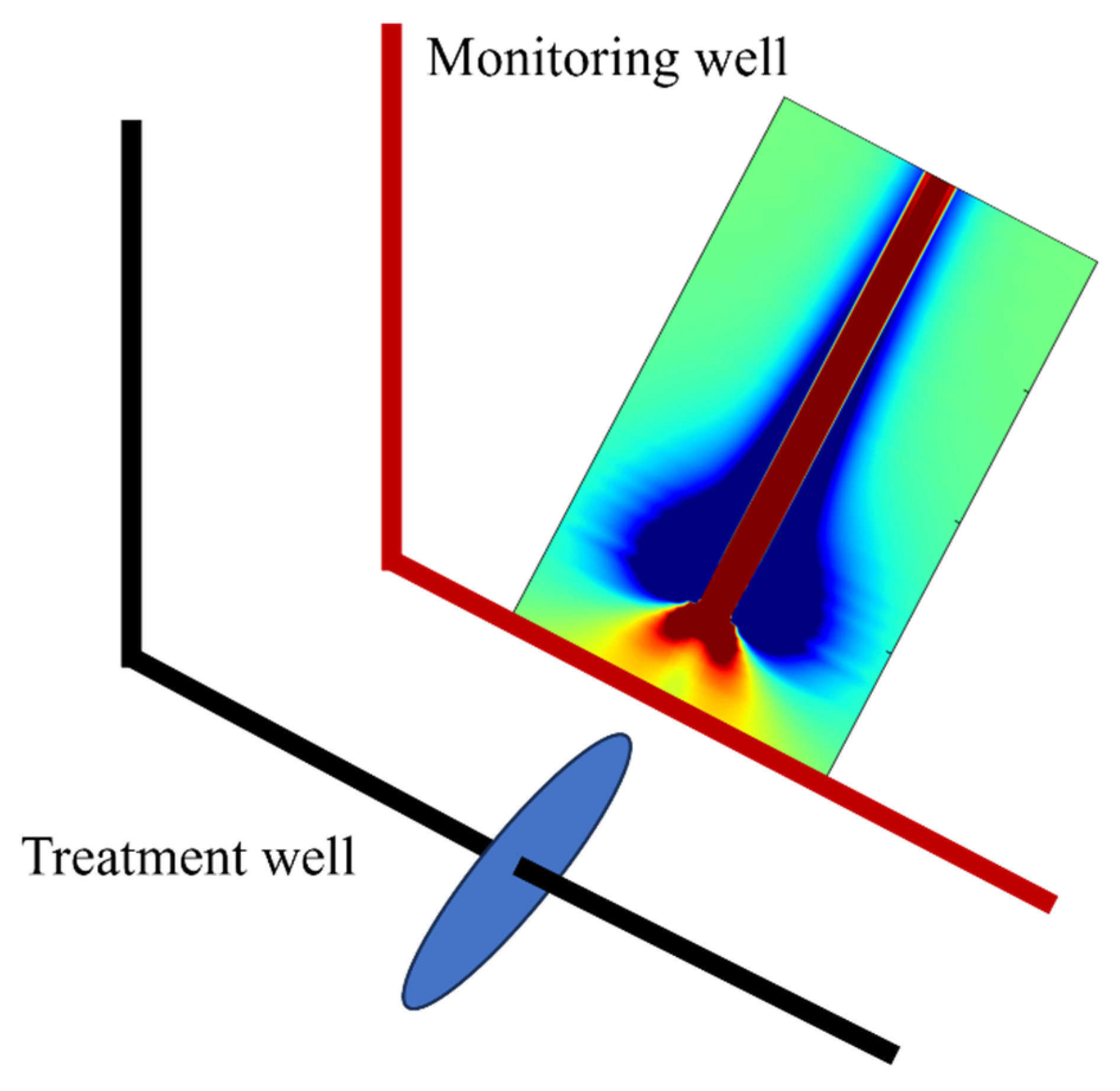
Figure 1. Schematic illustration of monitoring a vertical hydraulic fracture using LF-DAS deployed in a horizontal neighbor-well.
Processes 14 01380 g001
Figure 2. Hydraulic-fracture swarm: (a) core photograph; (b) unwrapped circumferential CT scan of cored section; (c) FMI-HD image of cored section; and (d) hydraulic-fracture swarm consisting of 22 fractures in a 20-ft section [20].
Processes 14 01380 g002
Figure 3. Schematic illustration of the relationship between gauge length and sample spacing along the fiber-optic cable.
Processes 14 01380 g003
Figure 4. L-curve for smoothing-parameter selection.
Processes 14 01380 g004
Figure 5. Schematic illustration of stress discretization in the semi-analytical method proposed by Mao et al. [36].
Processes 14 01380 g005
Figure 6. Schematic illustration of coordinate transformations between local fracture reference frames and the global coordinate system.
Processes 14 01380 g006
Figure 7. Schematic illustration of the numerical configuration used for validating the resolution enhancement model.
Processes 14 01380 g007
Figure 8. Results of synchronous fracture propagation.
Processes 14 01380 g008
Figure 9. Fiber-optic strain-rate waterfall plot for synchronous fracture propagation with a gauge length of 10 m.
Processes 14 01380 g009
Figure 10. Fiber-optic strain-rate waterfall plot for synchronous fracture propagation with a gauge length of 1 m.
Processes 14 01380 g010
Figure 11. Resolution-enhanced fiber-optic strain-rate waterfall plot for synchronous fracture propagation with a gauge length of 10 m.
Processes 14 01380 g011
Figure 12. Strain-rate profile comparison at representative time slices for the synchronous (top) and asynchronous (bottom) benchmarks.
Processes 14 01380 g012
Figure 13. Results of asynchronous fracture propagation.
Processes 14 01380 g013
Figure 14. Fiber-optic strain-rate waterfall plot for asynchronous fracture propagation with a gauge length of 10 m.
Processes 14 01380 g014
Figure 15. Fiber-optic strain-rate waterfall plot for asynchronous fracture propagation with a gauge length of 1 m.
Processes 14 01380 g015
Figure 16. Resolution-enhanced fiber-optic strain-rate waterfall plot for asynchronous fracture propagation with a gauge length of 10 m.
Processes 14 01380 g016
Figure 17. Noise sensitivity of the regularized inversion method at SNR = 30, 20, 10 and 5 dB.
Processes 14 01380 g017
Figure 18. Comparison of the regularized inversion method (top) and a Wiener filter (bottom) on the synchronous benchmark.
Processes 14 01380 g018
Figure 19. Neighbor-well fiber-optic strain-rate waterfall plots for gauge lengths of G = 2, 5, 10, and 15 m.
Processes 14 01380 g019
Figure 20. Resolution-enhanced neighbor-well fiber-optic strain-rate waterfall plots for gauge lengths of G = 2, 5, 10, and 15 m.
Processes 14 01380 g020
Figure 21. Neighbor-well fiber-optic strain-rate waterfall plots for different combinations of sample spacing and gauge length.
Processes 14 01380 g021
Figure 22. Resolution-enhanced neighbor-well fiber-optic strain-rate waterfall plots for different combinations of sample spacing and gauge length.
Processes 14 01380 g022
Figure 23. Dependence of inversion accuracy on gauge length G and sample spacing dl.
Processes 14 01380 g023
Figure 24. Well layout of the HFTS-2 field experiment [17].
Processes 14 01380 g024
Figure 25. Comparison of the original LF-DAS strain-rate waterfall plot (a) and the resolution-enhanced result (b) for Stage 22 of well B1H.
Processes 14 01380 g025
Figure 26. Comparison of the original LF-DAS strain-rate waterfall plot (a) and the resolution-enhanced result (b) for Stage 23 of well B1H.
Processes 14 01380 g026
Figure 27. Raw (blue) and enhanced (red) strain-rate profiles for HFTS-2 B1H Stage 22 at T = 1.53 h.
Processes 14 01380 g027
Figure 28. Raw (blue) and enhanced (red) strain-rate profiles for HFTS-2 B1H Stage 23 at T = 1.65 h.
Processes 14 01380 g028
Figure 29. Runtime breakdown of the regularized inversion method.
Processes 14 01380 g029
Table 1. Parameters of the regularized inversion method.
SymbolNameValueDescription
GGauge length10 m (synthetic)/7.147 m (HFTS-2)Spatial averaging window of a single LF-DAS channel
dlSample spacing1 m (synthetic)/1.021 m (HFTS-2)Along-fiber separation between consecutive channels
N = G/dlSub-segments per window10 (synthetic)/7 (HFTS-2)Number of high-resolution sub-segments per channel
KNumber of initial channels3Near-end seed size for the propagation passes
λTikhonov smoothing weight≈3.01 × 10⁻³Weight of the ‖Lx‖2 smoothness term
εRidge stabilizer1 × 10−10Numerical conditioning term
γ , β Prior weighting exponents1.0, 0.5Coverage and noise normalization exponents
σ 0 Reference noise scale1 × 10−8 s−1Normalization reference for the adaptive prior weight
Wavelet pre-denoisingdb4, soft, MADOptionalRecommended when SNR < 20 dB
Table 2. Fracture propagation parameters used in the validation of the resolution enhancement model.
Elastic Modulus (GPa)Poisson’s RatioInjection Rate
(m3/min)
Pumping Duration (min)Fracturing-Fluid Viscosity (mPa·s)Leakoff
Coefficient (m/s0.5)
Fixed Fracture Height (m)
21.40.263.26050.0000920
Table 3. Quantitative validation metrics for the synchronous and asynchronous benchmarks.
CaseMethodRMSE (s−1)MAE (s−1)Pearson rPeak Count Match (%)Peak Position MAE (m)
SynchronousRaw G = 10 m1.25 × 10−53.48 × 10−60.293320.95
SynchronousRegularized inversion9.05 × 10−61.09 × 10−60.8021000.50
AsynchronousRaw G = 10 m1.18 × 10−53.31 × 10−60.28513
AsynchronousRegularized inversion8.51 × 10−61.03 × 10−60.80895
Note: Self-consistency R2 (inverted field re-averaged vs. original G = 10 m observation) reaches 1.000 in both cases, confirming the inversion reproduces the input observation; the strict Pearson r values quoted above are against the high-resolution G = 1 m reference.
Table 4. Noise sensitivity of the regularized inversion method at four SNR levels.
SNR (dB)Self-Cons.
RMSE (s−1)
Self-Cons.
R2
Strict R2
(vs. G = 1 m)
Strict Pearson r
(vs. G = 1 m)
Peak Count Match (%)
301.33 × 10−81.0000.5630.77771
203.22 × 10−81.0000.3800.62424
109.95 × 10−80.999−1.4530.2943
51.77 × 10−70.999−5.8590.1753
Table 5. Comparison of the regularized inversion method and the Wiener filter at four SNR levels on the synchronous benchmark.
ScenarioMethodRMSE (s−1)MAE (s−1)Pearson rPeak Count Match (%)
Clean (no noise)Proposed9.05 × 10−61.09 × 10−60.802100
Clean (no noise)Wiener1.34 × 10−51.65 × 10−60.29668
SNR = 20 dB (+wavelet)Proposed1.10 × 10−51.84 × 10−60.67166
SNR = 20 dB (+wavelet)Wiener1.34 × 10−51.78 × 10−60.29729
SNR = 15 dB (+wavelet)Proposed1.18 × 10−52.05 × 10−60.57855
SNR = 15 dB (+wavelet)Wiener1.34 × 10−51.90 × 10−60.29734
SNR = 10 dB (+wavelet)Proposed1.28 × 10−52.33 × 10−60.42942
SNR = 10 dB (+wavelet)Wiener1.34 × 10−52.11 × 10−60.29521
Table 6. Effect of gauge length and sample spacing on inversion accuracy.
G (m)dl (m)G/dlEff. Resolution
(m)
Pearson r
(Inverted)
Peak Match
(Inverted, %)
Peak Match
(Raw, %)
RMSE (s−1)
51510.803010009.02 × 10−6
1011011.0000100321.40 × 10−7
102520.888097323.66 × 10−6
1511510.802810009.02 × 10−6
153530.6692055.88 × 10−6
204540.6040056.25 × 10−6
Table 7. Runtime and scalability of the regularized inversion method.
Datasetn_Tn_LLoad Time (s)A Cache Build (ms)Per-Step Solve (ms)Full-Stage Runtime (s)Throughput (Steps/s)
Synthetic G = 10 m benchmark602011.142.137.590.44137
HFTS-2 B1H Stage 2219816882.5221.845.2317.64112
Disclaimer/Publisher’s Note: The statements, opinions and data contained in all publications are solely those of the individual author(s) and contributor(s) and not of MDPI and/or the editor(s). MDPI and/or the editor(s) disclaim responsibility for any injury to people or property resulting from any ideas, methods, instructions or products referred to in the content.