Evaluating the Influence of Input Features for Data-Based Estimation of Wind Turbine Blade Deflections

Abstract

The increasing scale and structural flexibility of modern wind turbine rotors have made real-time monitoring and active control of blade tip deflection a critical requirement for ensuring operational safety, particularly regarding blade-tower clearance. Since direct measurement through physical sensors is often impractical due to high costs, installation difficulties and maintenance challenges, this work proposes a data-based framework for out-of-plane blade tip deflection estimation. The approach introduces a systematic and hierarchical input selection framework that evaluates sensor signal groups, ranging from standard SCADA measurements to configurations including auxiliary nacelle/tower sensors and dedicated blade-root instrumentation. By combining Spearman correlation and spectral coherence, the proposed framework ensures consistent representation of key turbine dynamics across all operating regions. This framework provides a structured trade-off between implementation feasibility and estimation fidelity, enabling tailored solutions for applications such as structural health monitoring and safety-critical active control. Compact Feedforward Neural Network (FNN) and Time-Delay Neural Network (TDNN) architectures, whose hyperparameters are optimized via Bayesian optimization, are employed to achieve high estimation accuracy while preserving computational efficiency. Evaluated through high-fidelity aeroelastic simulations of the NREL 5 MW turbine using the industry-standard FAST (Fatigue, Aerodynamics, Structures, and Turbulence) tool across all operating conditions, the approach achieves $R^2=0.894$ using SCADA-only inputs, $R^2=0.973$ when augmented with nacelle and tower-top sensors and a peak fidelity of $R^2=0.989$ using blade-root bending moment data. These results demonstrate that high-fidelity virtual sensing is attainable without blade instrumentation, providing a viable pathway for real-time tip clearance monitoring and fatigue mitigation. This directly enhances the operational resilience of wind energy systems and their contribution to the stability of renewable-dominated power grids.

1. Introduction

The global energy transition has driven wind energy technology toward unprecedented scales to minimize the Levelized Cost of Energy (LCoE). The industry has moved toward 15 MW turbines with rotor diameters exceeding 220 m and individual blade lengths surpassing 100 m, imposing new structural challenges [1]. While increasing the swept area is fundamental for higher energy capture, it exposes the rotor to the “square-cube law”, where structural mass tends to scale cubically while energy extraction scales only quadratically [2]. To overcome this, industry has adopted highly flexible architectures, utilizing advanced carbon-fiber composites and aeroelastic tailoring [3]. However, this inherent flexibility results in significant blade tip deflections, typically ranging from 3% to 10% of the blade length [4,5] and potentially reaching 15% to 20% under extreme wind conditions [6,7], effectively transforming the blade into a highly dynamic aeroelastic system. Excessive deflection poses immediate safety risks, most notably the violation of the tower clearance, which can lead to catastrophic tower strikes during extreme gusts or emergency stops [8]. Furthermore, large-amplitude cyclic oscillations accelerate fatigue damage accumulation, compromising the asset’s 25-year design life. Therefore, blade deflection is no longer a secondary structural variable but a critical state that directly constrains turbine design and operation. Consequently, real-time deflection estimation has evolved from a certification task into a mandatory requirement for Structural Health Monitoring (SHM) to avoid overly conservative design margins and enable active load-mitigating control strategies [9,10,11]. Ultimately, without reliable estimation, modern large-scale turbines must operate within reduced operational envelopes to ensure safety, thereby limiting energy capture and increasing the LCoE.

Direct measurement of blade tip deflection remains technically and economically challenging for mass deployment in the wind energy sector [12]. Instead of traditional Fiber Bragg Grating (FBG) sensors [13], novel non-contact methods such as ultra-wideband (UWB) sensing [14] and Digital Image Correlation (DIC) [15] have been proposed to bypass the limitations of direct blade instrumentation. Although FBG sensors provide high sensitivity and resilience to electromagnetic interference, instrumentation mounted near the blade tip faces significant operational hurdles in offshore environments, including restricted maintenance access and high costs of structural integration [12,13]. Proximity-based systems, such as Light Detection and Ranging (LiDAR) or photogrammetry, avoid direct blade instrumentation but introduce complexities regarding line-of-sight constraints, calibration and sensitivity to adverse weather conditions [16]. In contrast, strain gauges at the blade root continue to be the primary method for load assessment as they are available within standard load measurement systems, despite known issues with long-term signal drift, with studies now exploring strain-based estimation that reduces reliance on complex finite element models [17]. Root-bending moment measurements, specifically the out-of-plane (OoP) component, offer a pragmatic data source for high-fidelity virtual sensing (i.e., the inference of unmeasured physical states or signals from available sensor data), an approach increasingly adopted for fatigue damage tracking and condition-monitoring programs [12,13].

Early efforts relied on static machine learning models (e.g., feedforward neural networks, support vector regression) to estimate cumulative fatigue metrics such as the Damage Equivalent Load (DEL) [18,19]. While effective for condition monitoring, these approaches cannot reconstruct instantaneous blade tip deflections, limiting their utility for real-time safety-critical tasks such as Individual Pitch Control (IPC). More recent studies have explored dynamic models, such as Time-Delay Neural Network (TDNN) and Long Short-Term Memory (LSTM) architectures trained on high-fidelity simulations, to estimate and predict blade tip deflection from generator and nacelle data [12]. Furthermore, recent ensemble learning approaches have demonstrated high accuracy in predicting blade dynamics across various turbulence intensities [20], while LSTM architectures have been adopted to capture the temporal dependencies of blade tip motion [21]. High-fidelity digital shadows utilizing Kalman filtering have also been proposed to mirror blade behavior under complex inflow conditions, such as wake steering and yaw misalignment [22]. While Shubham Baisthakur and Fitzgerald [21] recently introduced a systematic feature selection approach based on mutual information, and Ismaiel [20] evaluated the generalization of ensemble models under varying turbulence intensities, these frameworks primarily rely on statistical mappings or require high-fidelity aerodynamic forces as inputs. Despite these advances, there is still a lack of a feature selection process grounded in the inherent physical dynamics and spectral characteristics of the blade [23], ensuring that the selected model inputs adequately capture the structural behavior of the system.

Table 1. Summary of prior studies on wind turbine blade monitoring and deflection estimation.

Study	Sensing/Input Strategy	Methodology	Key Focus/Gap Addressed
Naqash & Alam (2025) [13]	Direct (FBG/SHM)	Review	Failure mechanisms and vibration review.
Zhang et al. (2015) [14]	Direct (UWB)	Time-of-Flight Pulses	Non-contact tip-root distance sensing.
Jia et al. (2025) [15]	Direct (DIC)	Digital Image Corr.	Dynamic deformation regularity.
Ovenden et al. (2019) [16]	Proximity (LDS)/Strain	Laser Displacement	Ice, alignment and bolt-loosening detection.
Lee et al. (2017) [17]	Hybrid (Strain)	Modal Interpolation	Bypasses FE models for deflection.
Movsessian et al. (2021) [18]	Virtual (SCADA)	ANN (PCA, NCA)	Feature selection for tower fatigue (DEL).
De N Santos et al. (2023) [19]	Virtual (SCADA)	PINN (Physics-inf.)	Long-term fatigue estimation.
Dimitrov & Göçmen (2022) [12]	Virtual (SCADA/Load)	LSTM/TDNN	Time-series forecasting of tip deflection.
Ismaiel (2025) [20]	Virtual (SCADA/Wind)	Random Forest	Generalization across turbulence classes.
Baisthakur & Fitzgerald (2025) [21]	Virtual (LiDAR/SCADA)	LSTM (Mutual Info)	Systematic statistical feature selection.
Hadi et al. (2026) [22]	Digital Shadow	Kalman Filter	Complex inflow (wake and yaw misalignment).
Proposed Work	Virtual (SCADA→Aux→Root)	Spearman & Spectral Coherence + TDNN	Sensor trade-off evaluation for real-time OoP estimation.

provides a compact summary of these prior studies, highlighting the transition from direct sensing to data-driven virtual sensors and identifying the remaining gap in physics-informed feature selection.

This gap is particularly notable when contrasted with recent progress in tower deflection estimation. In that field, methodologies have evolved from traditional state observers and Kalman filters [11,24,25] to modern data-driven approaches utilizing TDNN and Recurrent Neural Network (RNN) architectures [26]. Particularly, Saavedra et al. [26] demonstrated that RNNs, combined with a rigorous input selection (Spearman correlation + spectral analysis), can estimate tower top displacements with high fidelity using only five widely available signals, including generator signals, pitch angle and nacelle acceleration. Yet, extending this approach to blade tip deflection is nontrivial. Unlike tower monitoring, blade tip acceleration is unavailable in standard turbine instrumentation suites. Furthermore, the task is complicated by the strong coupling between flapwise and edgewise modes (∼0.6–1.2 Hz) and an increased sensitivity to pitch transients. These dynamics are further influenced by the rotor’s azimuthal position, particularly due to the tower shadow effect at the fundamental rotational frequency (1P). Such complexities require an input selection process that accounts for the underlying physics of the coupled structural and control systems [27,28].

This paper addresses the challenge of real-time OoP blade tip deflection estimation through a data-driven framework that prioritizes input signal analysis over architectural complexity. The core contribution does not lie in the neural network design itself, but rather in a systematic and hierarchical evaluation of sensor configurations, from standard Supervisory Control and Data Acquisition (SCADA) signals to auxiliary sensors and, ultimately, to dedicated blade-root bending moment measurements. This approach enables a clear assessment of the trade-off between implementation feasibility and estimation fidelity for distinct operational objectives: basic structural health monitoring versus safety-critical active load control. The input selection process is rigorously grounded in a dual analysis of monotonic dependence via Spearman correlation and linear frequency-domain coupling through spectral coherence, following the methodology established in prior work on renewable energies [26,29]. This strategy identifies the minimal viable SCADA set and quantifies the significant performance gains from specific auxiliary measurements, notably nacelle yaw moments and tower-top accelerations, consistent with the signal classifications employed in research turbine database studies [30]. All estimators are trained and validated under operational uncertainty using high-fidelity, certified simulations from the National Renewable Energy Laboratory (NREL) FAST environment [31], across the full range of turbine operating regions and multiple turbulence realizations. The resulting virtual sensors demonstrate sufficient accuracy for practical deployment, confirming their viability for critical applications such as real-time tip clearance monitoring and fatigue load mitigation in next-generation, highly flexible wind turbines.

The remainder of this paper is structured as follows: Section 2 details the turbine model and generation dataset, Section 3 describes the data-based approach, including the selection of input features and the design of the neural network architectures. Section 4 and Section 5 report and discuss the results and Section 6 concludes the paper.

2. System Description and Data Generation

The present work employs the NREL 5MW reference onshore wind turbine [27], a three-bladed, upwind, horizontal-axis configuration widely adopted in the scientific community for controller design, load analysis and SHM research. The main technical specifications of this turbine are as follows: it has a nominal power of 5 MW, a rotor diameter of 126 m and a hub height of 90 m. Its open documentation, certified design basis and well-characterized aeroelastic response make it an ideal benchmark for methodological development. The turbine is operated under the standard controller architecture described in [32], comprising a gain-scheduled proportional–integral (PI) pitch controller (with anti-windup), a torque controller based on a lookup table tracking the optimal power coefficient and fixed yaw alignment.

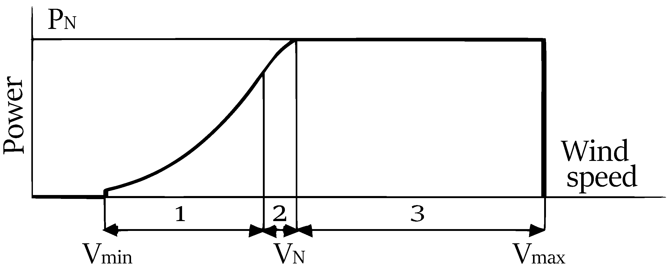
Operation is segmented into three wind-speed-dependent regimes (Figure 1): Region 1 (3–8 m/s), where pitch is fixed at the optimal angle and torque tracks the $C_p$-maximum curve; Region 2 (9–11.4 m/s), a transitional zone with active pitch engagement and more fatigue loading due to controllers interaction and increased turbulence penetration; and Region 3 (11.4–25 m/s), where pitch regulation maintains the rotor speed and torque at their nominal rated values. As illustrated in Figure 1, these regions are defined relative to key wind speed thresholds: the turbine remains inactive below $V_{\min }$ and above $V_{\max }$, with $P_N$ denoting the nominal power output achieved at the rated wind speed $V_N$. The power curve transitions smoothly from zero to $P_N$ in Region 1, remains constant at $P_N$ across Region 3, and exhibits maximum structural stress in Region 2 due to the dynamic interplay between aerodynamic loads and control actions.

The target signal is the blade tip deflection of blade 1, specifically the OoP (or flapwise) displacement. It is worth noting that blade 1 is selected without loss of generality, given the structural symmetry of the rotor and the proof-of-concept scope of this work. Extension to individual-blade estimation (e.g., for individual pitch control) would require parallel or multi-output architectures, beyond the present scope. This work focuses on OoP deflection, the dominant blade deformation component in terms of magnitude, which directly determines blade-tower clearance and constitutes a critical safety constraint in modern wind turbine operation. Although in-plane (IP) displacement is also present, it is excluded from the current analysis to prioritize the primary safety-critical deflection mode.

The OoP deflection of modern composite blades does not follow a simple quasi-static behavior. Instead, it arises from the combined contribution of stochastic aerodynamic forces associated with turbulent inflow and wake interactions, transient events such as sudden gusts or emergency shutdowns, and deterministic periodic loads [28]. These include 1P effects caused by wind shear and tower shadow, along with higher harmonics such as 3P. These excitations act on a highly flexible structure, giving rise to a dynamic response in which the dominant low-frequency envelope (associated with mean thrust variations) coexists with higher-frequency oscillations near the blade’s first flapwise natural frequency. Accurate estimation of OoP deflection therefore requires capturing not only the slow-varying trend that governs extreme loads and tip clearance but also the resonant dynamics that critically influence fatigue accumulation and the effectiveness of possible active load control strategies.

The dataset used in this work was generated through multiple dynamic simulations of the reference wind turbine using the Fatigue, Aerodynamics, Structures and Turbulence (FAST) software (v7.02.00d-bjj, NREL, Golden, CO, USA) [31]. FAST constitutes a high-fidelity, industry-validated simulation environment for modeling the fully coupled dynamics of modern wind turbines, including aerodynamic loading, structural flexibility, control logic and turbulent inflow. By numerically integrating the equations of motion, FAST generates time-resolved, physically consistent turbine responses across the full operational envelope. In this case, the turbine is subjected to mean hub-height wind speeds ranging from 3 to 25 m/s, ensuring that the simulations span all operating regimes to guarantee estimator robustness across the all operating regions. Wind inflow fields are generated with TurbSim (v1.06.00, NREL, Golden, CO, USA) [33] under turbulence Class B. For each 1 m/s step size discrete wind speed, six independent 10-min turbulent realizations are simulated. The use of turbulence Class B aligns with IEC 61400-1 [34] recommendations for load analysis under normal power production conditions (e.g., DLC 1.1 and DLC 1.2). Although this study focuses on normal operation scenarios, the proposed estimation framework is not restricted to a specific turbulence class and can be extended to alternative site-specific turbulence conditions provided that representative training datasets are available. A complete summary of the FAST model configuration, turbine properties, structural degrees of freedom, control parameters and TurbSim settings is provided in Appendix A for reproducibility.

From the set of outputs generated by FAST, a collection of measurable and physically interpretable signals is considered during the feature selection process (Section 3.1 and Section 3.2).

Table 2. Summary of FAST-derived signals employed.

Signal (FAST Name)	Physical Meaning	Units
Control- and SCADA-available signals
GenSpeed	Generator rotational speed	rad/s
GenTq	Generator torque	Nm
BldPitch1	Pitch angle of blade 1	deg
Azimuth	Rotor azimuth angle (generator reference)	deg
Structural response signals (tower)
TTDspFA	Tower-top FA displacement	m
TTDspSS	Tower-top SS displacement	m
YawBrTAxp	Tower-top FA acceleration	m/s2
YawBrTAyp	Tower-top SS acceleration	m/s2
TwrBsMyt	Tower-base FA bending moment	Nm
TwrBsMxt	Tower-base SS bending moment	Nm
Nacelle-level torque (often instrumented in research turbines)
YawBrMxp	Nacelle FA yaw moment	Nm
YawBrMyp	Nacelle SS yaw moment	Nm
Blade-specific structural signals
RootMyc1	Blade root out-of-plane bending moment	Nm
OoPDefl1	Blade 1 tip out-of-plane (flapwise) deflection (target signal)	m
Environmental input
WindVxi	Hub-height longitudinal wind speed (inertial frame)	m/s

lists the identifiers for the time series employed, along with their physical meaning and units, categorized by origin and practical availability. These range from standard SCADA and control signals to structural response variables typically available only via additional instrumentation or post-processing. This signal set serves as the foundation for defining the input subsets evaluated during the estimator design phase.

3. Data-Based Estimation

This section details the methodology for developing and evaluating the data-based estimators. A systematic analysis of the candidate input signals is first conducted to assess their informativeness, redundancy and practical availability. Based on this analysis, the signals are organized into different input groups to evaluate the trade-off between implementation feasibility and estimation performance. The following subsections describe the neural network architectures, the Bayesian optimization framework employed for hyperparameter tuning and sensitivity analysis, and the corresponding training and evaluation scheme.

3.1. Input Signal Analysis

The design of a data-based virtual sensor relies fundamentally on a rigorous understanding of how measurable signals relate, both statistically and dynamically, to the target signal. To this end, a twofold analysis is conducted [26,29]. Monotonic relationships are evaluated using Spearman’s correlation coefficient. Frequency-domain linear dependencies are assessed through spectral coherence, enabling the identification of inputs that contain relevant information within the blade’s critical modal bands. This dual analysis is evaluated separately for each operational region to respect regime-specific physics, avoiding the pitfall of global metrics masking local deficiencies where estimation consistently underperforms.

3.1.1. Spearman Correlation Analysis

Spearman’s correlation coefficient is utilized to assess the monotonic relationships between potential input variables and the target signal. This non-parametric approach is preferred over alternatives such as Pearson’s correlation because it captures both linear and nonlinear monotonic associations, which is essential given the inherent nonlinearities of wind turbine aeroelastic response. Moreover, Spearman’s coefficient does not assume normally distributed data and is less sensitive to extreme values, making it better suited for identifying features with significant predictive relevance.

Although correlation does not establish causality, it provides an essential preliminary measure of feature importance. Furthermore, the analysis of inter-variable correlation indices allows for the identification and exclusion of collinear signal pairs, ensuring that the focus remains on the most relevant information regarding the output variable.

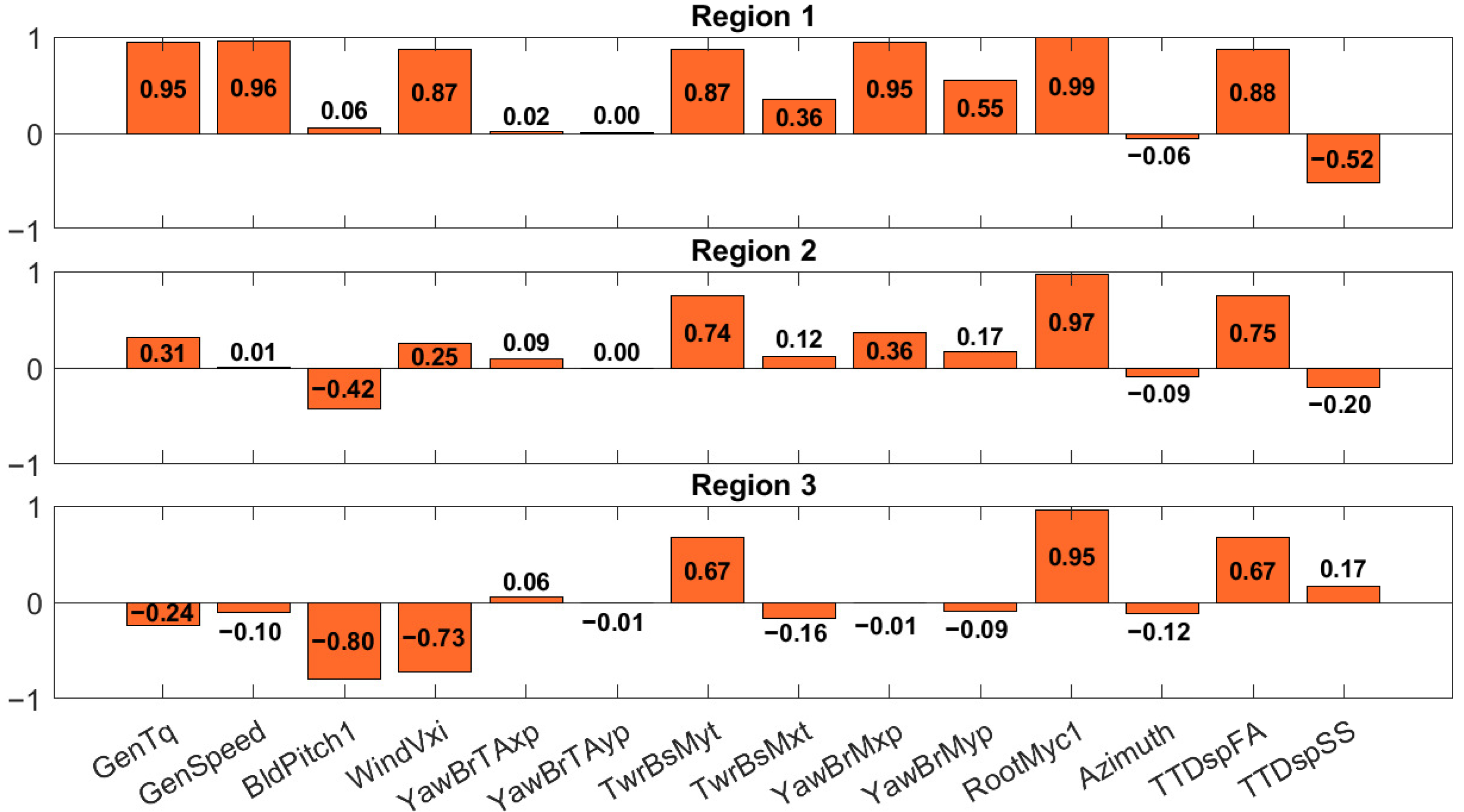
Figure 2 shows the correlation indices against the target variable (OoPDefl1) for the different variables and operating regions of the wind turbine. A first observation shows that the RootMyc1 signal consistently demonstrates exceptional correlation with target signal across all regions (0.99 in Region 1, 0.97 in Region 2 and 0.95 in Region 3), the strongest monotonic relationship with blade tip deflection. However, as a dedicated strain gauge measurement at the blade root, it is typically unavailable in commercial turbines and primarily used in research prototypes [14]. Conversely, the analysis of the remaining signals reveals distinct patterns across the three operational regimes, reflecting the fundamentally different dynamics inherent to each region.

In Region 1, high correlations (>0.85) are observed with generator-related signals (GenSpeed at 0.96 and GenTq at 0.95), alongside tower-base torque (TwrBsMyt at 0.87), yaw-bearing torque (YawBrMxp at 0.95) and tower top deflection (TTDspFA at 0.88). This pattern aligns with the operational characteristics of Region 1, where the turbine operates with fixed pitch and maximum energy capture, making generator dynamics the primary driver of blade deflection. The strong correlation with WindVxi (0.87) further confirms the dominance of free wind-driven thrust variations in this region.

Region 2 exhibits a different correlation profile, with the strongest relationships observed with TwrBsMyt (0.74), TTDspFA (0.75), YawBrMxp (0.36) and GenTq (0.31). Notably, blade pitch (BldPitch1) begins to show a significant negative correlation (−0.42), reflecting the active pitch control engagement in this transition region. In this region, correlation values around (≥0.3) must be interpreted in a relative sense, reflecting the comparative contribution of different variables rather than representing an absolute significance threshold. These lower values suggest more complex dynamics, where multiple factors jointly influence the deflection response.

In Region 3, the correlation pattern shifts again, with RootMyc1 achieving the highest correlation, followed by TwrBsMyt and TTDspFA (both at 0.67). The negative correlations with BldPitch1 (−0.80) and WindVxi (−0.73) reflect the dominant influence of pitch regulation in maintaining constant power output under high-wind conditions.

Concluding, while tower-base signals like TwrBsMyt and TTDspFA maintain strong relationships across all regions, their relative importance shifts, with generator signals dominating in Region 1 and pitch-related dynamics becoming more prominent in Regions 2 and 3. Additionally, it is important to consider that as observed in previous works [26], while Spearman’s correlation effectively captures monotonic dependencies, it remains insensitive to fully capture complex non-linear relationships and phase-specific dependencies. These dynamics are often not reflected in time-domain statistical indices but become evident when analyzed in the frequency domain.

3.1.2. Spectral Coherence Analysis

To complement the monotonic relationship assessment from Spearman’s correlation, spectral coherence analysis is conducted to identify frequency-specific couplings between the inputs and the OoPDefl1 signal. Unlike correlation metrics, coherence quantifies linear dependence at each frequency, revealing which signals carry information in critical dynamic bands (e.g., the tower shadow effect near 0.2 Hz under rated conditions and the first flapwise mode at 0.6–0.7 Hz). The magnitude-squared coherence (MSC) $C_{xy}\left(f\right)$ is defined as [35]:

$$C_{xy}\left(f\right)={\displaystyle \frac{|P_{xy}{\left(f\right)|}^2}{P_{xx}\left(f\right)P_{yy}\left(f\right)}},$$

(1)

where $P_{xy}\left(f\right)$ is the cross-spectral density between signals $x\left(t\right)$ and $y\left(t\right)$, and $P_{xx}\left(f\right)$ and $P_{yy}\left(f\right)$ are their respective power spectral densities.

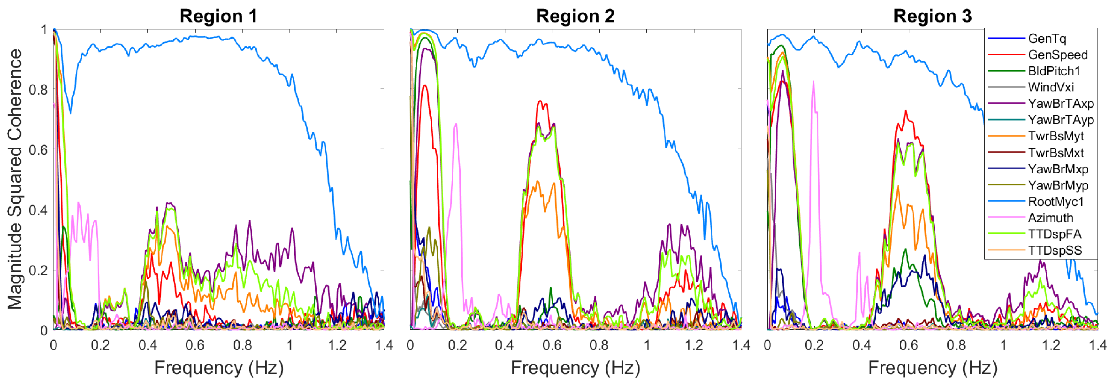
The MSC between the input features and the target deflection variable is illustrated in Figure 3 for the three operating regions. These plots serve as a graphical method to assess the linear relationship between the signals across the frequency spectrum, where a higher Area Under the Curve (AUC) indicates a stronger linear correlation over a broader frequency band. The 1.4 Hz frequency range is selected to capture the full blade dynamic bandwidth, consistent with the spectral content observed in the Power Spectral Density (PSD) of the deflection signal.

The analysis is organized into specific frequency bands tailored to the structural properties of the NREL 5MW reference turbine. These bands are selected according to the blade’s structural natural frequencies as defined in [27], covering the low-frequency base region (0–0.3 Hz), as well as the first and second structural modes (specifically 0.3–0.9 Hz and 0.9–1.4 Hz, respectively). These bands coincide with the zones and peaks of high spectral coherence observed in Figure 3. To quantify these relationships,

Table 3. AUC of the MSC between input signals and OoPDefl1, categorized by operating region and frequency band.

Signal ↓/Freq. (Hz) →	Region 1			Region 2				Region 3
	0 Hz	0–0.3	0.3–1.4	0 Hz	0–0.3	0.3–0.9	0.9–1.4	0 Hz	0–0.3	0.3–0.9	0.9–1.4
GenTq	1.00	0.08	0.01	0.96	0.13	0.01	0.01	0.75	0.06	0.01	0.00
GenSpeed	0.96	0.13	0.05	0.99	0.30	0.21	0.07	0.76	0.35	0.24	0.04
BldPitch1	0.05	0.06	0.01	0.50	0.41	0.02	0.01	0.40	0.38	0.07	0.02
WindVxi	0.96	0.06	0.01	0.98	0.07	0.01	0.01	0.57	0.09	0.00	0.00
YawBrTAxp	0.00	0.04	0.19	0.02	0.36	0.23	0.15	0.00	0.28	0.23	0.09
YawBrTAyp	0.00	0.00	0.01	0.02	0.03	0.01	0.01	0.00	0.00	0.01	0.01
TwrBsMyt	0.99	0.21	0.09	1.00	0.46	0.16	0.03	0.91	0.40	0.15	0.02
TwrBsMxt	0.98	0.05	0.01	0.96	0.08	0.01	0.01	0.63	0.03	0.01	0.00
YawBrMxp	1.00	0.08	0.03	0.96	0.12	0.03	0.03	0.75	0.07	0.08	0.01
YawBrMyp	0.04	0.01	0.02	0.78	0.12	0.01	0.01	0.53	0.03	0.00	0.00
RootMyc1	1.00	0.91	0.75	1.00	0.96	0.93	0.51	0.95	0.95	0.87	0.39
Azimuth	0.75	0.20	0.01	0.99	0.18	0.02	0.01	0.76	0.17	0.02	0.01
TTDspFA	0.99	0.21	0.13	1.00	0.46	0.22	0.10	0.90	0.39	0.22	0.05
TTDspSS	0.99	0.06	0.01	0.96	0.10	0.01	0.01	0.68	0.03	0.01	0.00

shows the normalized spectral coherence AUC computed for each band. This yields a coefficient ranging from 0 to 1, representing the proportion of the theoretical maximum coherence achieved within that specific frequency interval. Notably, the 0 Hz column represents the exact coherence value at 0 Hz (not an AUC), which is crucial for capturing the quasi-static component of blade deflection. This slow-varying trend defines the mean loading state essential for DEL calculations, even when such low-frequency components are poorly captured by standard time-domain correlation metrics.

A primary observation from the figure is that, again, the RootMyc1 variable exhibits the highest coherence across all regions. This is attributed to its role as a dedicated moment sensor, which is physically coupled with the blade’s structural response. Regarding the other variables, the coherence patterns reveal up to three distinct frequency bands where different input signals demonstrate significant coupling with the OoP deflection. While these three intervals are clearly discernible in Regions 2 and 3, the separation is less prominent in Region 1, where the dynamics are primarily captured by two main bands. Consequently, in Table 3, the 0.3–0.9 Hz and 0.9–1.4 Hz ranges are consolidated into a single 0.3–1.4 Hz band. The characteristics of these frequency ranges are detailed below.

In the low-frequency band (0–0.3 Hz), the results align with the rotational 1P frequency (≈0.2 Hz) at rated speed, capturing periodic excitations such as wind shear and the tower shadow effect as perceived by the rotating blades. Therefore, signals such as Azimuth, TwrBsMyt and TTDspFA show notable coherence in this range. Furthermore, within this band for Regions 2 and 3, BldPitch1 exhibits a notable frequency contribution, consistent with the activation of pitch control for rotor speed regulation.

The middle band (0.3–0.9 Hz) encompasses both the 3P blade-pass frequency (≈0.6 Hz) and the first flapwise mode of the blade (≈0.697 Hz), as documented in the NREL 5MW reference model [27]. In this interval, YawBrTAxp, TTDspFA, TwrBsMyt and GenSpeed demonstrate the notable coupling, with AUC values ranging from 0.16 to 0.25 across regions, reflecting their role as indirect proxies for the primary elastic response of the rotor and tower.

Finally, the high-frequency band (0.9–1.4 Hz) contains the first edgewise mode (≈1.08 Hz) [27] and higher-order harmonics. In this region, YawBrTAxp consistently dominates with AUC values between 0.09 and 0.19 highlighting the sensitivity of nacelle accelerations to transient structural dynamics and higher-frequency vibrations that are decoupled from the low-frequency aerodynamic loading. This is followed by TTDspFA with values between 0.05 and 0.13 and a smaller contribution from GenSpeed, which exhibits values ranging from 0.04 to 0.07.

Table 3 reveals a critical insight previously overlooked in the visual analysis: signals like GenTq and YawBrMxp, while exhibiting high Spearman correlation (0.998 and 0.998 in Region 1, respectively), demonstrate their strongest coherence at 0 Hz, with minimal contribution in the dynamic bands. This could be useful for estimating the deflection trends, at the cost of not capturing high-frequency oscillations. 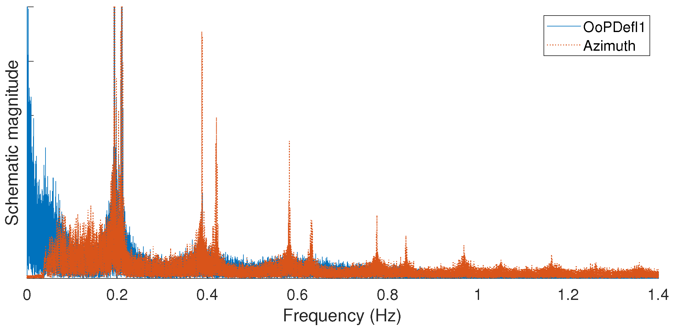Additionally, the Azimuth signal, while appearing to have negligible monotonic correlation due to its periodic nature (0–360°), exhibits significant coherence at 0.2 Hz, making the signal essential for modeling periodic transients despite its modest overall correlation coefficient. The coherence patterns underscore the necessity of incorporating Azimuth into the estimator, as it is a primary feature source for this frequency band. As illustrated in Figure 4, the spectral content of the Azimuth signal aligns with one of the most prominent energy peaks in the target deflection signal, capturing a substantial portion of the system’s deterministic periodic response. It should be noted that the spectral amplitudes in Figure 4 have been rescaled to arbitrary units for illustrative purposes. This normalization facilitates the visual comparison of the frequency distribution across different input variables, ensuring that their relative contributions to the frequency bands of interest are discernible despite their different physical units and magnitudes.

3.2. Input Feature Grouping and Selection

Based on the correlation and spectral analyses presented in Section 3.1, three hierarchically structured input configurations are defined. The incremental inclusion of variables is guided not only by quantitative metrics (absolute Spearman correlation coefficients and spectral coherence amplitude) but also by physical interpretability and practical sensor availability in standard turbine instrumentation. Variables exhibiting negligible correlation and no discernible coherence peaks in the frequency bands of interest (e.g., YawBrTAyp) are excluded in most input groups, while those showing strong statistical linkage and physically meaningful spectral content are retained. Each group reflects a distinct trade-off between implementation feasibility and estimation fidelity, targeting different deployment scenarios: standard SCADA-only monitoring, augmented sensing with auxiliary tower-top instrumentation and high-fidelity prototyping via dedicated blade-root sensors. These configurations are summarized in

Table 4. Inputs groups definition, categorized by sensor configuration.

Group ID	Variables Included
SCADA-only
S0	Azimuth, BldPitch1, GenSpeed
S1	Azimuth, BldPitch1, GenTq
S2	Azimuth, BldPitch1, GenSpeed, GenTq
SCADA + auxiliary sensors
A0	S2 + TwrBsMyt
A1	S2 + YawBrTAxp
A2	S2 + YawBrMxp
A3	S2 + TwrBsMyt, YawBrTAxp
A4	S2 + TwrBsMyt, YawBrTAxp, YawBrMxp
A5	S2 + TwrBsMyt, YawBrTAxp, YawBrMxp, TwrBsMxt, YawBrTAyp, YawBrMyp
Dedicated-sensor configuration
D0	RootMyc1
D1	RootMyc1, Azimuth
D2	RootMyc1 + S2
D3	RootMyc1 + A4

, where each group is identified by its representative ID and variable composition.

The first category, SCADA-only (groups S0–S2 in the table), includes signals routinely logged by industrial control systems. This set comprises GenTq and GenSpeed, which exhibit the highest correlation among SCADA signals in Region 1 (>0.96). Notably, GenSpeed is the only SCADA variable showing non-negligible coherence above 0.3 Hz, whereas GenTq dominates the zero-frequency component. In addition, Azimuth is included to capture its distinctive coherence peak at 0.2 Hz, and BldPitch1 is considered due to its increasing correlation in the 0–0.3 Hz band as pitch control becomes active. It is important to note that the classification of these operational and control variables as standard SCADA components is consistent with recent literature on wind turbine health monitoring frameworks [30].

The second category, SCADA + auxiliary sensors, augments the base set to account for the bandwidth not captured in the S0–S2 configurations, primarily at high frequencies. Although TTDspFA exhibits strong correlation and coherence throughout the frequency range of interest, it is intentionally excluded from the primary auxiliary set due to its practical unavailability in field deployments. Instead, three physically measurable tower signals are prioritized. The tower-base FA moment (TwrBsMyt) is selected due to its high coherence across all operating regions and its multicollinearity with FA deflection. The nacelle FA acceleration (YawBrTAxp) is chosen for its dominant contribution within the 0.3–1.4 Hz frequency range. The nacelle FA yaw moment (YawBrMxp) is included to reinforce the static and low-frequency contributions, where its Spearman correlation exceeds 0.96 in Regions 1 and 2 and its coherence peaks at 0 Hz. Groups (A0–A5) are constructed incrementally, from single additions (A0–A2) to full combinations (A5), with the latter incorporating side-to-side signal counterparts (TwrBsMxt, YawBrTAyp, YawBrMyp) to account for torsional and asymmetric dynamics.

The third and final category, dedicated-sensor configuration, uses the blade-root OoP bending moment RootMyc1 as the primary input. The use of this signal is physically grounded, as the root bending moment is the fundamental driver of the flapwise structural response. In the simulation environment, this variable represents the pure OoP component, which is intrinsically coupled with blade tip deflection, a relationship that may require coordinate transformation in real-world applications to account for pitch-induced sensor misalignment. Its inclusion follows an empirical progression: starting from a minimal estimator D0 (RootMyc1 alone), followed by D1 adding Azimuth to recover periodic transients, D2 incorporating the full SCADA core and finally, D3 using the tower-top auxiliary set, establishing a high-fidelity reference for performance benchmarking.

This structured approach ensures that the subsequent modeling and evaluation phases can be conducted within well-defined constraints, enabling direct comparison of performance across different sensor availability scenarios.

3.3. Neural Network Architectures

Given the instantaneous nature of the blade deflection estimation problem, a TDNN architecture is adopted as the core modeling approach. This choice is justified by literature and practical considerations. Specifically, Dimitrov and Göçmen [12] demonstrated that for the estimation task, feedforward architectures with time-lagged inputs achieve comparable performance to recurrent networks, such as LSTM, while significantly reducing computational latency. This efficiency is critical for wind turbine controllers, where estimators must operate within strict real-time constraints to match the control strategy’s sampling frequency. Since FNN and TDNN inference involves only deterministic matrix operations and nonlinear activations evaluation, its execution time on standard industrial hardware, such as PLCs or embedded systems, is in the microsecond range, representing a negligible fraction of the control cycle [36,37,38]. Furthermore, preliminary tests confirmed that more complex RNN and LSTM architectures offered no significant accuracy gains to justify their higher computational overhead compared to the TDNN.

Two architectures are evaluated. The first is a Feedforward Neural Network (FNN) used as a baseline, mapping instantaneous inputs $\mathbf{x}\left(t\right)$ directly to the estimate $\widehat{y}\left(t\right)$, based on one or more hidden layers with hyperbolic tangent (TanH) activation. The second is a TDNN, where inputs are augmented with N past samples to form $\mathbf{X}\left(t\right)=\left[\mathbf{x}\right(t),\mathbf{x}(t-1),\dots ,\mathbf{x}(t-N\left)\right]$, processed by L hidden layers of M neurons (with TanH activation) followed by a linear output layer. In this way, the TDNN explicitly incorporates temporal context without sacrificing robustness and speed. Regarding the internal architecture, the TanH activation function is employed in the hidden layers due to its zero-centered output and smooth nonlinear mapping, which facilitate stable gradient propagation and effective learning in shallow regression networks [39]. A linear activation function is used in the output layer to allow the network to estimate the continuous range of blade tip deflections without saturation effects.

3.4. Training and Evaluation Scheme

The dataset comprises 138 10-min turbulent realizations generated with FAST [31] under class B turbulence conditions (Section 2). While simulations are initially sampled at 66.67 Hz, the signals are downsampled to 16.67 Hz. This sampling frequency remains well above the Nyquist–Shannon criterion for the blade’s first flapwise mode ($f_{1\mathrm{F}}\approx 0.7$ Hz). Furthermore, to maintain a balanced training set, Region 3 simulations are performed using 1 m/s steps between 13 and 16 m/s, as well as at specific mean wind speeds of 18, 20, 22 and 24 m/s. This sampling strategy is adopted because Region 3 represents the widest operational range. Finally, all input features are scaled to the $[0,1]$ interval using min–max normalization, ensuring numerical stability during gradient-based optimization.

The training/validation partition follows a turbulence-seed separation: for each wind speed in the dataset, four out of six stochastic realizations are assigned to training and the remaining two to validation. The network weights are optimized using the Levenberg–Marquardt algorithm, which is selected for its rapid convergence and its ability to navigate complex error surfaces with multiple local minima [40]. This optimization method integrates the stability of gradient descent with the speed of the Gauss–Newton approach, ensuring superior computational performance. The primary objective of the training process is to minimize the Mean Square Error (MSE) cost function, iteratively adjusting the synaptic weights to reduce the discrepancy between the estimated and true deflection values. Finally, the estimation accuracy is assessed using Coefficient of Determination (R²) and Normalized Root Mean Square Error (NRMSE) (Section 4). Following the methodology of Dimitrov and Göçmen [12], the NRMSE is normalized by the standard deviation of the target signal, rather than its mean, to ensure a robust and consistent evaluation for variables that may approach a zero-mean value.

3.5. Bayesian Optimization and Sensitivity Analysis

To systematically determine the TDNN hyperparameters while avoiding overfitting, a Bayesian optimization framework is employed. This approach efficiently explores the hyperparameter space by building a probabilistic surrogate model (Gaussian process) of the validation loss (MSE), selecting new candidates via the expected improvement acquisition function. The optimization targets three critical hyperparameters: the number of hidden layers L (range: 1–16), the hidden layer size M (range: 2–16), which controls the model capacity via the number of neurons in each hidden layer, and the memory depth N (range: 1–64), representing the number of past samples included. The procedure is conducted in two sequential stages to decouple architectural complexity from temporal context length. The complete setup and results are summarized in

Table 5. Summary of Bayesian optimization setup, search ranges and final hyperparameter selection.

Stage	Hyperparameter	Search Range	Selected Value
1. NN architecture      (FNN model)	L: number of hidden layers	1–16	1
	M: hidden layer size (neurons)	2–16	9
2. Memory depth      (TDNN model)	N: past input samples considered	1–64	48
Optimization Settings		Detail
Objective metric	Mean Squared Error (MSE) on validation set
Surrogate model	Gaussian Process (GP) regression
Kernel function	Matérn 5/2 with Automatic Relevance Determination (ARD)
Acquisition function	Expected Improvement Plus (EI+)

.

It should be noted that the hyperparameter optimization is performed using a reduced but representative dataset to balance computational cost and informativeness. Specifically, simulations of 5 min duration (instead of 10) are employed, with one turbulence realization for training and one for validation per wind speed. This setup enables rapid evaluation of candidate architectures during the Bayesian search while preserving the spectral content and statistical characteristics of the original dataset. The objective of this tuning phase is not to identify a globally optimal architecture, but rather to select a suitable and consistent model configuration that enables meaningful comparison across input groups in the subsequent analysis while capturing the dominant dynamics of blade tip deflection under normal operating conditions. The resulting hyperparameters are subsequently validated using the full 10-min test set, confirming their effectiveness beyond the reduced tuning dataset.

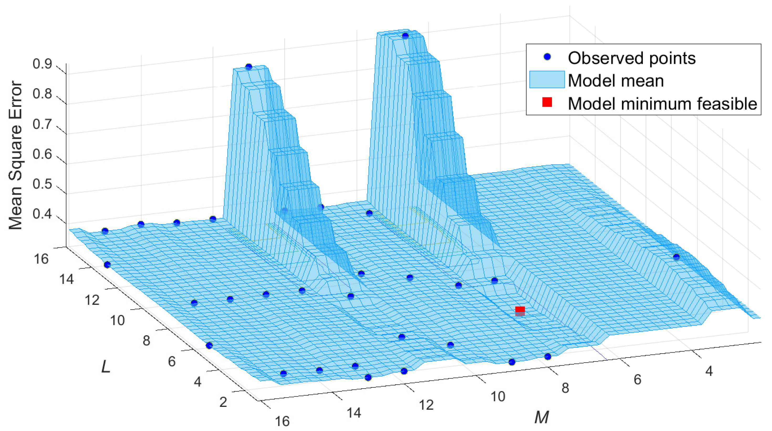
In the first stage, the shared architectural hyperparameters, L and M, are optimized on the static FNN (no time delays), as its simpler structure makes performance more sensitive to changes in capacity. Figure 5 shows the optimization trajectory: each blue point corresponds to an independent training run (30 iterations) and the light blue surface represents the surrogate model. The analysis identifies $L=1$ and $M=9$ as the optimal trade-off between accuracy and complexity (observed MSE = 0.354), with diminishing returns beyond 10 neurons and marginally improved performance from adding more layers.

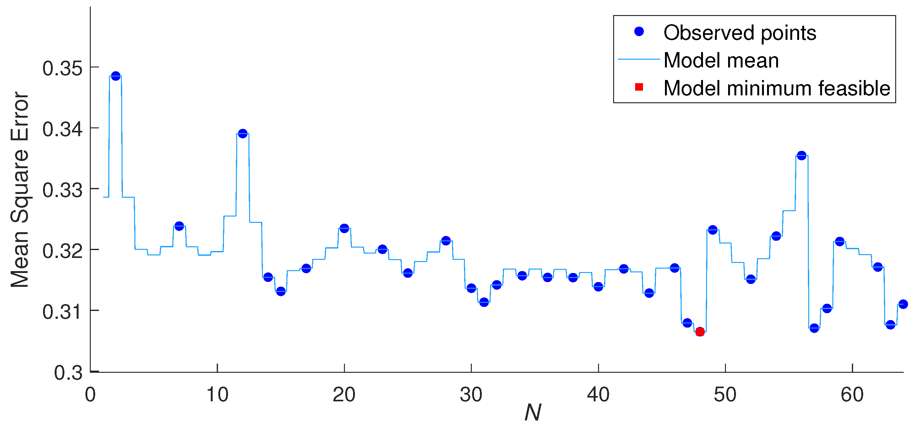
In the second stage, the memory depth N is optimized for the TDNN (16 iterations), preserving the $L=1$ and $M=9$ architecture found above to ensure a fair comparison. Figure 6 illustrates that while performance variation remains minimal across individual runs (blue points), the region between $N=31$ and $N=48$ displays greater stability. Although the algorithm identifies a relatively better performance at the formal minimum of $N=48$, $N=31$ is selected to prioritize model simplicity without a significant sacrifice in estimation accuracy. Increasing the number of delays beyond $N=48$ leads to greater variability in the results, as seen in the subsequent error spikes, likely due to an elevated sensitivity to random weight initialization. This suggests that the added complexity, resulting from the increased number of synaptic weights when incorporating additional samples, does not justify the marginal performance gains observed at higher memory depths.

In summary, the Bayesian optimization explored a broad search space, evaluating architectures ranging from a single hidden layer to 16 layers, with varying past input samples. By selecting a compact structure, model complexity is controlled and the computational footprint remains suitable for real-time control integration. The resulting hyperparameters ($L=1$, $M=9$, $N=31$) are fixed for all subsequent estimator training and evaluation.

4. Results

Table 6. Estimation performance of FNN and TDNN models across input configurations and datasets. Metrics reported: NRMSE and R². Best values per family are highlighted in bold.

Group	Model	NRMSE				${\mathit{R}}^2$
		R1	R2	R3	All	R1	R2	R3	All
SCADA-only
S0	FNN	0.323	0.616	0.420	0.369	0.896	0.621	0.824	0.864
	TDNN	0.312	0.555	0.400	0.347	0.903	0.692	0.840	0.880
S1	FNN	0.366	0.624	0.414	0.374	0.866	0.611	0.829	0.860
	TDNN	0.314	0.531	0.431	0.358	0.901	0.718	0.814	0.871
S2	FNN	0.291	0.502	0.409	0.339	0.915	0.748	0.833	0.885
	TDNN	0.265	0.427	0.414	0.325	0.930	0.818	0.829	0.894
SCADA + auxiliary sensors
A0	FNN	0.287	0.485	0.403	0.332	0.918	0.765	0.838	0.890
	TDNN	0.269	0.417	0.405	0.320	0.928	0.826	0.836	0.898
A1	FNN	0.283	0.487	0.400	0.330	0.920	0.763	0.840	0.891
	TDNN	0.261	0.423	0.385	0.309	0.932	0.821	0.852	0.905
A2	FNN	0.266	0.466	0.383	0.315	0.929	0.783	0.853	0.901
	TDNN	0.217	0.333	0.321	0.254	0.953	0.889	0.897	0.935
A3	FNN	0.261	0.436	0.378	0.307	0.932	0.810	0.857	0.906
	TDNN	0.255	0.378	0.400	0.309	0.935	0.857	0.840	0.904
A4	FNN	0.234	0.398	0.351	0.283	0.945	0.841	0.877	0.920
	TDNN	0.199	0.268	0.357	0.264	0.960	0.928	0.872	0.931
A5	FNN	0.156	0.294	0.268	0.212	0.976	0.913	0.928	0.955
	TDNN	0.122	0.183	0.220	0.164	0.985	0.966	0.952	0.973
Dedicated-sensor configuration
D0	FNN	0.367	0.293	0.368	0.298	0.865	0.914	0.865	0.911
	TDNN	0.146	0.223	0.371	0.261	0.979	0.950	0.863	0.932
D1	FNN	0.366	0.284	0.340	0.282	0.866	0.919	0.884	0.920
	TDNN	0.133	0.216	0.345	0.244	0.982	0.953	0.881	0.940
D2	FNN	0.103	0.181	0.162	0.129	0.989	0.967	0.974	0.983
	TDNN	0.085	0.150	0.142	0.111	0.993	0.978	0.980	0.988
D3	FNN	0.102	0.180	0.160	0.128	0.990	0.968	0.975	0.984
	TDNN	0.082	0.142	0.137	0.107	0.993	0.980	0.981	0.989

summarizes the estimation performance (NRMSE and R²) across all input configurations (Table 4), evaluated on the test set. Results are reported for both the static FNN and the time-delay variant (TDNN), across the three operational regions (R1, R2, R3) and the aggregated dataset (all regions). Each group family, SCADA-only (S0–S2), SCADA + auxiliary sensors (A0–A5) and dedicated-sensor (D0–D3), is grouped accordingly, with the best-performing configuration within each group highlighted in bold.

The results in Table 6 confirm that although the performance gains are relatively modest, the TDNN consistently outperforms its static counterpart FNN across all input groups and operational regions, despite only marginal improvements in some cases.

In the SCADA-only category, the best-performing configuration overall is S2-TDNN, achieving an NRMSE of 0.325 and R² of 0.894 on the full dataset. Among the three operating regions, Region 2 exhibits the highest error levels (NRMSE = 0.427, R² = 0.818), although the performance difference with respect to Region 3 is moderate, while Region 1 shows the best metrics. This is attributed to the transitional nature of the control strategy in this region, where the switching between generator torque control and pitch regulation, coupled with intermittent pitch saturation and non-minimum phase dynamics, results in a more complex and non-stationary input–output relationship compared to the purely torque-driven (Region 1) or pitch-limited (Region 3) regimes. Regarding the use of generator speed (S0) or torque (S1), no significant difference in estimator performance is observed. However, the simultaneous inclusion of both signals (S2) generally yields enhanced estimation accuracy for the majority of regions. It is worth noting that while S2-TDNN performs best for Regions 1 and 2, the S0-TDNN estimator achieves a marginally better performance specifically for Region 3 (NRMSE = 0.400), though this comes at the cost of notably worse results in Region 2 (R2 = 0.692 for S0-TDNN compared to 0.818 for S2-TDNN).

When auxiliary sensors are incorporated, estimation performance improves markedly. Within the SCADA + auxiliary sensors groups, A5-TDNN achieves the highest fidelity, achieving an overall NRMSE value of 0.164 and R² of 0.973. Notably, Regions 2 and 3 exhibit the most significant gains, with NRMSE reduced to 0.183 (R² = 0.966) and 0.220 (R² = 0.952), respectively, confirming that tower-top dynamics effectively recover high-frequency content absent in the first family group. A closer inspection of the incremental configurations (A0–A2) reveals that the nacelle FA yaw moment (YawBrMxp) yields the largest single-sensor improvement over the best SCADA-only baseline (S2-TDNN), reducing NRMSE by 21% (from 0.325 to 0.254 in the full dataset). This contribution reappears in group A4, where adding YawBrMxp to the A3 configuration (itself combining TwrBsMyt and YawBrTAxp) further elevates performance. Moreover, the inclusion of side-to-side counterparts (TwrBsMxt, YawBrTAyp, YawBrMyp), as in group A5, produces a discernible gain, increasing R2 by up to 8% in Region 3 relative to A3, underscoring the value of capturing asymmetric and torsional dynamics.

Finally, the dedicated-sensor configurations establish the performance upper bound. D3-TDNN yields the lowest overall error (NRMSE = 0.107, R² = 0.989). As expected, the blade-root bending moment exhibits strong coupling with blade tip deflection: even the minimal configuration D0 (RootMyc1 only) attains R² = 0.911 overall. However, this single-sensor setup does not outperform the performance of the richer SCADA + auxiliary configuration A5-TDNN, primarily due to significantly higher errors in Region 3. Significant gains emerge only when RootMyc1 is augmented with SCADA variables D2 (R² = 0.983 for FNN, R² = 0.988 for TDNN) or further enriched with auxiliary tower-top signals D3 (R² = 0.984 for FNN and R² = 0.989 for TDNN), though the latter delivers only marginal improvement over D2.

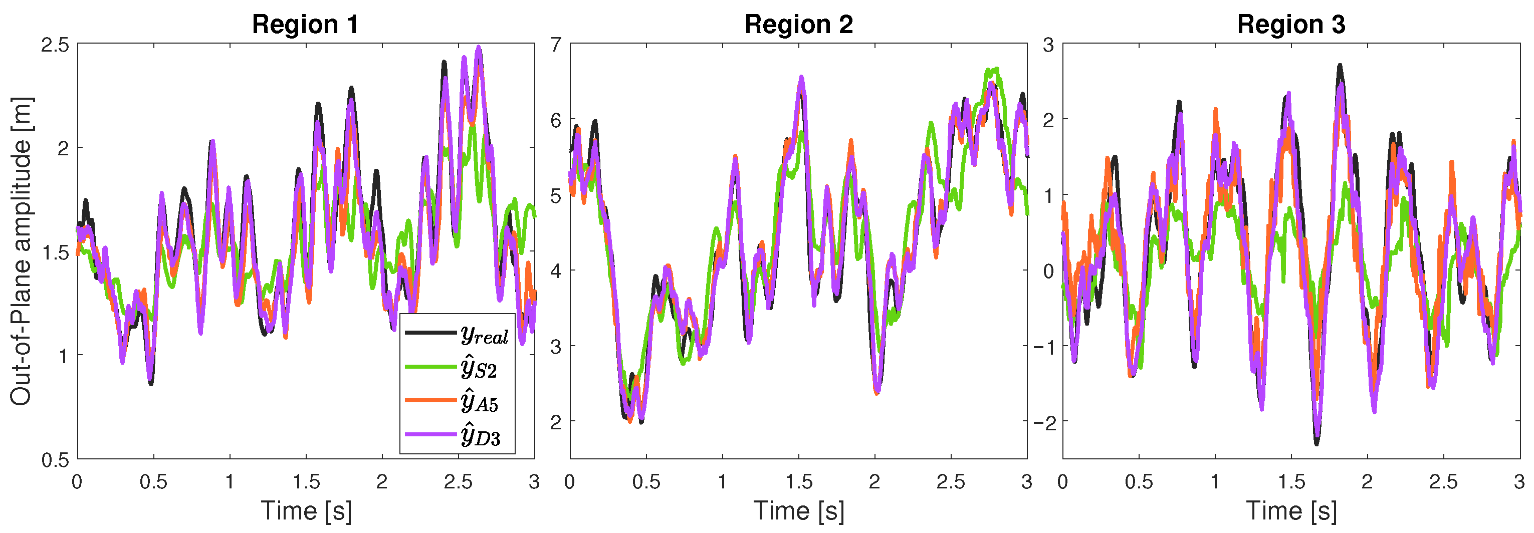
Additionally, Figure 7 and Figure 8 provide complementary time- and frequency-domain validation of the top-performing configurations: S2-TDNN (SCADA-only), A5-TDNN (SCADA + auxiliary) and D3-TDNN (dedicated-sensor). As shown in the temporal series (Figure 7), S2-TDNN captures only the low-frequency envelope of the deflection, behaving like a moving-average filter, with notable degradation in Regions 1 and 3, where high-frequency correlation is lower. In contrast, A5-TDNN successfully reconstructs both the quasi-static trend and a substantial portion of the dynamic oscillations across all regions, confirming its ability to recover interest bandwidth. 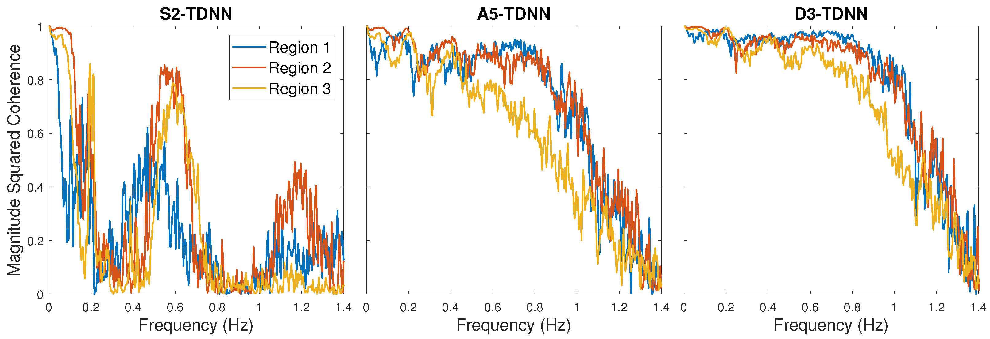D3-TDNN achieves the best tracking to the ground truth, particularly in Regions 2 and 3, thanks to the physical fidelity of RootMyc1. This hierarchy is further corroborated in the output coherence spectra (Figure 8): S2 exhibits strong coherence only below 0.2 Hz and in first flapwise mode frequency, A5 extends coherent coupling up to 0.8 Hz (covering completely the first flapwise mode) and D3 maintains near-unity coherence across the entire 0–1.4 Hz operational band, validating the quantitative superiority observed in Table 6.

5. Discussion

The consistent, though modest, superiority of the TDNN over the static FNN across all sensor configurations confirms that temporal context is useful for high-fidelity deflection estimation. However, the relatively small performance gap suggests that in latency-constrained applications, a well-designed FNN may be preferable when auxiliary sensors are available, trading marginal accuracy gains for computational simplicity. In contrast, when only SCADA signals are accessible or computational resources are not a constraint, the TDNN’s ability to recover partial dynamic content makes it the preferred option for feasible real-time control design.

From an implementation standpoint, SCADA-only estimators, while sufficient for monitoring quasi-static trends (e.g., mean thrust, long-term structural drift), lack the bandwidth required for comprehensive fatigue analysis or active load control, as evidenced by their poor high-frequency coherence (Figure 8). In contrast, the SCADA + auxiliary sensor family (particularly A5-TDNN) achieves fidelity levels compatible with active load control without requiring blade instrumentation. The nacelle FA yaw moment (YawBrMxp) emerges as the most informative auxiliary signal among the three analyzed sensors. Its combination with the remaining sensor signals and their side-to-side counterparts captures torsional dynamics otherwise missed, enabling performance that even surpasses the dedicated-sensor baseline (D0). Only when the SCADA or auxiliary sensor signals are incorporated into the dedicated set (D2/D3) is full-bandwidth reconstruction achieved.

It is important to note that the estimators are trained and validated using datasets generated under IEC Class B turbulence, representative of normal power production conditions. While this selection reflects typical operational scenarios relevant for structural health monitoring and control-support applications, extreme operating conditions defined in other IEC design load cases (e.g., fault events, emergency shutdowns or parked turbine scenarios) involve significantly different aerodynamic and control dynamics [10,41]. Extending the proposed framework to such conditions would require dedicated training datasets capturing those operational states. Nevertheless, the data-driven methodology itself remains applicable and can be adapted to alternative turbulence classes and extreme load cases through appropriate dataset expansion. This is further supported by recent findings showing that models trained on IEC Class B turbulence can generalize to other turbulence classes. Ismaiel [20] reported suitable R² values for flapwise deflection estimation across Classes A and C, suggesting that representative operational data (Class B) can provide a reliable basis for real-time monitoring under most common operating conditions.

The findings are consistent with the results reported by Dimitrov and Göçmen [12], who achieved high accuracy using a subgroup of 11 input signals (including tower torques, control signals and tower-top acceleration) together with a large $2\times 60$ TDNN architecture. The authors reported an NRMSE of 0.649 for an input subset comparable to the SCADA-only configuration and 0.162 when using all signals, similar to the SCADA + auxiliary sensor setup. By contrast, the results of the present work demonstrate that a significantly more compact $1\times 9$ TDNN, relying on fewer inputs, can provide superior performance. Specifically, the proposed estimator achieves a substantially lower error in the SCADA-only regime (NRMSE of 0.325) and practically equivalent accuracy in the SCADA + auxiliary sensor configuration (NRMSE of 0.164). Additionally, this approach provides instantaneous deflection, thereby facilitating its potential use in active control, in contrast to previous studies [18,19], which focus on 10-min statistics or DEL.

Regarding the choice of FNN and TDNN architectures over more complex recurrent architectures such as RNNs and LSTMs, preliminary experiments were conducted under the same input configurations and within the same hyperparameter search space derived from the TDNN optimization process. For the best-performing input groups (S2, A5, and D3), the obtained validation results yielded $R^2$ values of 0.793, 0.981, and 0.990 for the RNN and $R^2$ values of 0.881, 0.926, and 0.976 for the LSTM across the three configurations, respectively. The observed performance did not demonstrate consistent improvements over the proposed TDNN and, in some cases, even underperformed relative to it. These results suggest that the temporal dependencies relevant to blade tip deflection estimation are predominantly short-term and can be effectively captured using a fixed-length temporal window. Since the TDNN does not rely on explicit internal states but instead performs nonlinear mappings of recent input samples, it achieves greater computational efficiency by avoiding recursive internal dynamics. Consequently, the advanced long-term memory mechanisms embedded in LSTM structures do not appear to be fully exploited in this application. These observations are consistent with previous findings in the literature [26], where simpler recurrent or feedforward dynamic architectures were shown to perform comparably to LSTM-based models in problems dominated by short-term dynamics. Therefore, the TDNN represents a pragmatic balance between temporal expressiveness and real-time deployability for the present estimation task. Nevertheless, as the framework evolves toward deeper or more expressive architectures and more demanding operating scenarios, the incorporation of stabilization mechanisms such as residual connections or normalization layers, as well as hybrid physics–machine learning paradigms embedding aerodynamic constraints [42], emerges as a promising direction to further enhance robustness, numerical stability, and physical interpretability.

Finally, it is important to note that although tower-top displacement (TTDspFA) was excluded from the auxiliary sensor set due to its limited availability in standard turbine instrumentation, it was nevertheless evaluated under the premise that this signal can be virtually reconstructed from existing nacelle accelerometers and SCADA signals using data-based estimators, as demonstrated in [26]. Preliminary tests indicate that its inclusion in the A5-TDNN configuration further improves performance, reducing NRMSE to 0.151 and increasing R2 to 0.977. While this numerical improvement may appear modest, TTDspFA provides a direct measure of the global structural response to wind loading. As such, if routinely available, it could potentially replace several indirect inputs, thereby simplifying the sensor suite while preserving estimation fidelity. This suggests that future integration of tower-top displacement estimates could offer a practical pathway to leverage this signal without requiring additional hardware.

6. Conclusions

This work demonstrates that accurate estimation of blade tip OoP deflection is achievable using data-based estimators, providing performance that scales from trend-level monitoring to high-fidelity reconstruction, both with and without dedicated blade instrumentation. The input selection methodology, guided by Spearman correlation and spectral coherence analysis, ensures consistency across critical frequency bands, while a Bayesian optimization framework enables the systematic selection of model hyperparameters. All findings are based on high-fidelity simulations under IEC Class B turbulence and normal operating conditions. These assumptions define the boundaries of the present results and provide a basis for future experimental validation under real-world operating conditions.

Future work will prioritize the integration of virtual tower-top displacement (e.g., FA and SS estimated from nacelle accelerations and SCADA signals, as in [26]), following the significant potential observed in preliminary tests. Additionally, the implementation of these estimators within a closed-loop individual pitch control scheme for active deflection and load mitigation will be explored. The methodology will also be extended to address estimator generalization across multiple turbulence classes and selected extreme IEC design load cases to assess robustness under off-nominal operating conditions. Furthermore, the adoption of advanced architectural features, such as residual connections and normalization layers, and the exploration of physics–machine learning hybrid paradigms will be investigated to enhance physical interpretability and accuracy in highly non-linear regions. Finally, the framework will be expanded to full aeroelastic load estimation (including edgewise deflection and root moments) to enable DEL optimization and remaining useful life assessment under realistic turbulence conditions.