1. Introduction
Hydropower is a dispatchable renewable-energy resource that can complement variable generation from wind and solar power. In addition to conventional reservoir and run-of-river plants, compact hydrokinetic turbines can recover kinetic energy directly from flowing rivers and canals without requiring the hydraulic head and major civil structures associated with traditional hydropower installations. Their modularity makes them relevant for distributed generation, but it also changes the operating and maintenance problem: a deployment may contain multiple geographically dispersed units, each operating under continuously varying flow and environmental conditions. Reviews of river and marine hydrokinetic conversion describe both the technical potential of these devices and the control challenges arising from variable inflow, electromechanical conversion, and site-specific operating conditions [
1,
2,
3,
4].
For a distributed hydrokinetic system, energy yield depends not only on the available resource but also on the ability of the generator and controller to maintain effective mechanical-to-electrical energy conversion. Short interruptions that would be minor in a single laboratory test can accumulate across time and across a fleet of turbines. Because small units are expected to operate with limited local maintenance and limited computing resources, operational abnormalities should ideally be identified close to the asset and early enough for a safe controller response. This requirement differs from conventional condition monitoring that is designed primarily for slowly developing component degradation and periodic maintenance planning.
The broader operational motivation concerns transient power-loss anomalies; one such condition is the event of free-spin. For the hydrokinetic device used in the study, free-spin occurs when the rotor remains in motion while measured electrical power is zero. The classifier target is deliberately narrower: it predicts the first exact transition of measured power to zero from the two preceding observations. The classifier is therefore described as an exact-zero-power onset or power-lapse predictor rather than a direct free-spin classifier. Predictive maintenance (PdM) is used in the restricted sense of short-horizon condition monitoring, not prediction of long-term degradation or remaining useful life [
5].
Condition-monitoring research for rotating energy systems provides a useful methodological starting point. Vibration analysis and supervisory control and data acquisition (SCADA) data have long been used to identify gearbox, generator, and drivetrain abnormalities [
6,
7]. Machine-learning approaches extend this idea by learning relationships among operating variables and fault labels from historical telemetry [
8,
9]. Reviews of wind-turbine condition monitoring show a broad range of statistical, signal-processing, and supervised-learning approaches [
10,
11]. Nevertheless, the dominant examples concern large wind turbines, relatively slow degradation, and centralized data analysis. Direct transfer to a kilowatt-scale hydrokinetic device is not automatic because the event horizon, sensor configuration, available labelled events, and embedded-computing budget are different.
A second aspect of the problem is power control. The turbine investigated here uses a torque-based maximum power point tracking (MPPT) strategy. A configurable torque multiplier changes the generator torque reference and therefore the operating balance between rotor motion, electrical loading, power capture, and the occurrence of free-spin. A multiplier selected solely to maximize average power could place the unit in an undesirable operating region, while an overly conservative setting could reduce energy capture. The control problem is consequently multi-criteria in engineering terms, even though the available experiment evaluated only a small number of discrete multiplier settings [
12].
The available literature and project evidence expose three connected gaps. First, published hydrokinetic studies provide limited evidence on sub-second or second-scale precursors to transient power-loss events. Second, many predictive-maintenance models are evaluated offline and do not explicitly consider the inference and response constraints of an embedded controller. Third, predictive monitoring and control-parameter selection are often treated as separate problems, even though both depend on the same electromechanical telemetry and influence the same operational state. These gaps motivate an applied investigation that combines a lightweight early-warning model with empirical examination of a torque-control parameter [
13].
The objective of this study is to determine whether the two preceding per-rotor telemetry observations contain sufficient information to classify the next exact-zero-power onset and to integrate this monitoring capability with field-informed selection of the maximum-power-point controller multiplier. The prediction task uses a six-feature Random Forest classifier [
14], which is compared with alternative model families, while Shapley additive explanations (SHAP) are used to inspect feature reliance [
15,
16]. The power-optimization component combines recorded multiplier comparisons with the engineering assessment that led to deployment of 0.82.
The contributions are:
- (1)
Automated construction of episode-controlled pre-event examples from operational telemetry;
- (2)
A compact temporal and relational representation for short-horizon power-lapse prediction;
- (3)
Leakage-resistant chronological validation and comparison of multiple model families;
- (4)
Corrected six-feature SHAP interpretation;
- (5)
Field evaluation of an engineering-selected 0.82 operating configuration. The paper focuses on the predictive-monitoring and power-optimization methodology without disclosing unnecessary proprietary mechanical, firmware, or site details.
The methodology follows five functional stages: operational data acquisition, event-oriented processing, predictive learning and interpretation, controller-setting evaluation, and field execution with feedback. The available evidence includes chronological classifier evaluation and archived field excerpts for four controller settings, including the deployed 0.82 configuration. Automatic classifier-triggered actuation and continuous retraining remain future extensions rather than reported results.
2. Related Work
2.1. Hydrokinetic Energy Conversion and Control
Hydrokinetic energy-conversion systems extract kinetic energy from river or tidal currents rather than relying on a hydraulic head. Khan et al. [
1] review horizontal- and vertical-axis devices and identify resource variability, structural loading, conversion efficiency, and deployment conditions as central design considerations. Chen et al. [
2] similarly discuss marine-current energy systems, including generator and control challenges. Although river and marine-current devices differ in scale and environment, both require the electrical load to be coordinated with the hydrodynamic operating state.
Maximum-power-point control is commonly used to regulate this coordination. In a torque-controlled generator, the commanded electromagnetic torque determines the electrical loading applied to the rotor. The controller must capture available energy without driving the system into unstable, inefficient, or mechanically undesirable operation. Existing hydrokinetic literature has emphasized model-based control and perturb-and-observe strategies [
2]. The present study is narrower: it examines a configurable multiplier applied to an existing torque reference and uses field telemetry to compare operating outcomes. Rather than proposing a new hydrodynamic turbine model or a universal maximum-power-point algorithm, it demonstrates the application of an AI-supported decision-making framework to predictive condition monitoring and power-control optimization in a hydrokinetic case study [
3,
12].
2.2. Condition Monitoring and Predictive Modelling
Hydrokinetic and tidal-turbine research increasingly addresses fault detection under variable inflow and restricted maintenance access. Benchmark models have been proposed for in-stream turbine fault detection and fault-tolerant control [
17], while rotor-imbalance detection has been investigated under turbulent-flow and optimal tip-speed-ratio operation [
18]. Hydrokinetic MPPT research has also demonstrated the importance of coordinating electrical loading with water velocity and rotor speed [
19].
Recent hydropower monitoring studies further demonstrate data-driven condition assessment and PdM using operational sensor data [
20,
21,
22]. These studies complement the broader maintenance-policy research in [
23]. Wind-turbine studies [
7,
8,
9,
10,
11] are retained as neighbouring methodological context, but direct transfer is limited by differences in scale, event horizon, sensing, and operating environment.
The classifier target differs from many conventional fault labels because it is generated automatically from an exact signal transition rather than from a confirmed maintenance record. This supports scalable labelling but creates methodological risks: overlapping windows, non-independent comparison examples, and random partitioning can inflate apparent performance. Event definition, sample construction, and split strategy are therefore central to the validity of the evaluation [
13,
24,
25].
2.3. Tree Ensembles and Explainable Machine Learning
Random Forest combines predictions from multiple Decision Trees and is well suited to nonlinear relationships among tabular sensor variables [
14]. Its applicability to energy-conversion problems has also been demonstrated alongside other machine-learning approaches for data-driven estimation of power-electronic operating losses [
26]. It requires less feature scaling than many distance-based methods and can represent interactions among power, torque, and their ratio. Gradient-boosted trees provide an alternative ensemble approach [
27], while recurrent models can represent longer temporal dependencies. The original analysis architecture used Random Forest, but model-family selection should be supported by comparative evaluation rather than architectural continuity alone.
Interpretability is particularly important when a prediction may affect controller behaviour. SHAP expresses a prediction as a baseline plus feature-level contributions derived from Shapley values [
15]. TreeExplainer provides an efficient implementation for tree ensembles [
16]. SHAP can show whether a model is relying on physically plausible variables, but it does not establish causality and does not by itself make a model intrinsically interpretable. Rudin [
28] cautions against treating post hoc explanations as a substitute for transparent modelling in high-stakes settings. Accordingly, SHAP is used here as a diagnostic aid: attribution patterns are compared with expected electromechanical behaviour, and operational conclusions are not based on SHAP alone.
2.4. Research Gap and Position of This Study
The literature listed shows the support of the use of sensor telemetry, tree ensembles, and attribution methods, but thus far does not directly resolve the specific combination examined in this study, being a short-duration power-loss event on a small river turbine, with prediction using only the immediately preceding samples, and empirical adjustment of a torque multiplier on the same asset.
The contribution is therefore application-specific rather than a claim that Random Forest or SHAP is methodologically new. Rather, the study demonstrates the practical value of integrating SHAP-based model interpretability into AI-supported decision-making frameworks for renewable energy systems, using the operation of hydrokinetic turbines as a case study. By identifying and interpreting the operational parameters influencing model predictions, the study illustrates how explainable AI can support condition monitoring and power-control optimization. Its scientific value lies in transparent event construction, temporally defensible evaluation, interpretable model predictions, and a clear separation between measured configurations, regression estimates, and field validation.
3. System and Dataset
3.1. Methodological System Boundary
The experimental platform comprises an operational distributed horizontal-axis hydrokinetic energy-conversion system deployed in a European river environment. The data used in this study was obtained from the operational telemetry and control infrastructure of an industrial hydrokinetic turbine deployment.
For scientific reporting, the relevant system boundary comprises two rotor channels, an on-site CM4-based embedded computing unit, an operational telemetry store, offline data-processing routines, and a torque-based maximum-power-point controller with an adjustable control multiplier. The analysis is restricted to variables and system components required to evaluate the investigated control and operational behaviour. Information not required for reproducibility of the presented methodology is outside the scope of this study and is therefore omitted.
The measured variables used by the processing pipeline include input voltage, input current, motor current, and rotor speed. Derived electrical power and rotor torque are calculated during SQL-to-CSV processing as P = −V_in I_in and τ = −1.17 I_motor, respectively. For the binary prediction model, we remove the negative sign convention by taking the absolute values of power and torque.
Figure 1 presents the functional data path.
3.2. Sampling Frequency and Sequential Structure
Operational telemetry was collected directly from the deployed hydrokinetic system through the on-site CM4-based embedded computing infrastructure. Raw telemetry was stored by the operational system and subsequently exported manually for offline preprocessing, machine-learning analysis, SHAP interpretation, and control-parameter evaluation.
Analysis of the raw timestamps yields a median interval of approximately 0.624 s for each rotor, corresponding to an effective per-rotor rate of approximately 1.6025 Hz. Because the two rotor channels are interleaved, the combined table contains approximately 3.205 records s−1. The SQL-processing notebook parses the PostgreSQL COPY block and writes the ordered records directly to processed CSV files; it does not resample or aggregate the sequence.
For a model using the two observations preceding an onset at t, the interval from t − 2 to t is approximately 1.25 s, while the most recent input at t − 1 is approximately 0.624 s before the onset. The method therefore uses a short history spanning about 1.25 s; it should not be described as providing a uniformly less-than-one-second prediction horizon.
3.3. Operational Labels and High-Speed Indicator
Two distinct operational indicators are used and are not treated as mathematically equivalent. Here, r denotes the rotor channel, t the observation index, and ω
r,t the measured rotor speed in eRPM. A project-level high-speed anomaly flag is based only on rotor speed:
The binary classifier does not predict this high-speed flag. After power and torque have been converted to absolute values, its target is the first exact-zero-power transition:
The corrected classifier retains the exact-zero-power target in Equation (2), while repeated transitions occurring within 10 s are treated as one episode. In the multiplier-1.0 recording, 337 raw transitions produce 279 independent episode onsets. The operational free-spin comparison is evaluated separately using the domain definition ωr,t > 0 with power equal to zero. The two labels are related operationally but are not treated as mathematically equivalent.
3.4. Datasets
The processed data contain two equally represented rotor streams and no missing cells or duplicate rotor/timestamp pairs. Four archived controller-setting excerpts are available, with different dates and durations.
Table 1 reports their sizes and sampling characteristics.
The 0.82 deployment excerpt contains 25,590 rows, equally divided between the two rotors, and approximately 2.20 h of operation per rotor. The SQL table does not contain a controller-setting field; setting attribution is based on the archived source filename and engineering deployment record.
The archived excerpts contain no flow velocity, discharge, water-level, or equivalent hydrodynamic normalization variable. Comparisons among controller settings are therefore observational and may reflect both the selected setting and differences in operating conditions.
4. Methodology
4.1. Analysis Overview
The study contains two related analyses and a field-implementation stage. First, a six-feature Random Forest predicts exact-zero-power onset under chronological validation and is compared with four alternative model families. Second, field excerpts recorded at controller settings 0.8, 0.9, 1.0, as well as the final value of 0.82 are compared using power and exposure-normalized free-spin occurrence. The predictive and optimization components use the same electromechanical telemetry, although automatic prediction-triggered actuation was not evaluated.
4.2. Processing Applied to the Binary Classifier
The SQL-to-CSV pipeline parses the raw database export, converts timestamp and sensor fields to numeric values, calculates power and torque, generates the RPM-based flag in Equation (1), and computes quartile-based descriptive flags. It retains all rows. The binary training notebook then sorts observations by rotor and timestamp, replaces power and torque with their absolute values, and constructs lagged windows.
No feature scaling, imputation, Z-score removal, interquartile-range removal, or manual relabelling is applied to the
Table 2 classifier. The processed multiplier datasets contain no missing cells and no duplicate rotor/timestamp pairs. Quartile flags created during preprocessing are not inputs to the binary model.
4.3. Positive-Window Construction
The multiplier-1.0 sequence contains 337 raw exact-zero-power transitions: 188 for Rotor 1 and 149 for Rotor 2. To prevent repeated zero/nonzero toggles within one disturbance from being treated as independent events, transitions separated by 10 s or less are grouped. The 10 s refractory period provides a conservative separation relative to the sub-second sampling interval and the short, repeated transitions observed during anomaly recovery. This produces 279 episode onsets (155 for Rotor 1 and 124 for Rotor 2). Each episode contributes one positive feature vector containing the observations at t − 2 and t − 1.
For absolute power P and absolute torque τ, the relational feature is calculated with a numerical stabilizer:
The six-dimensional input vector associated with onset t is
Rotor speed, current, voltage, first differences, rolling statistics, and t − 3/t − 4 lags are not features of this binary model.
4.4. Negative Windows and Class Balancing
Normal-operation windows require three consecutive positive-power observations, rotor speed within 0 < ωr,t ≤ 6000 eRPM and inter-sample gaps below 2 s. Candidate normal windows are excluded when any of their observations lies within 10 s of a zero-power, high-RPM, or nonpositive-RPM observation.
Normal windows are sampled from both rotors and throughout the complete recording. Each retained negative window consumes three consecutive source rows and does not overlap another negative window or a positive feature window. The final dataset contains 36,636 non-overlapping windows: 279 positive episode onsets and 36,357 normal-operation windows. Non-overlapping means that retained windows do not share source rows; adjacent windows may nevertheless remain serially correlated. Class weighting is applied during training to address the naturally rare onset class.
4.5. Training, Validation, and Test Split
Samples are divided chronologically according to elapsed recording time. The first 60% is used for training, the next 20% for validation, and the final 20% is retained as an untouched test period. The resulting partitions contain 21,861 training windows, 7375 validation windows, and 7400 test windows. The test period contains 35 positive onsets and 7365 normal-operation windows.
Both rotors are represented in every partition. Model configuration is selected using training and validation data only. The final-period labels are not used for model or threshold selection, preventing overlapping-window leakage and providing a future-period assessment within the available recording.
4.6. Random Forest Configuration
Logistic Regression, Decision Tree, Random Forest, radial-basis-function Support Vector Machine, and Histogram Gradient Boosting are compared. A modest candidate search is performed using the validation period. The retained Random Forest contains 500 trees, uses square-root feature subsampling, a minimum leaf size of three, balanced-subsample class weighting, and random seed 20260922.
Table 2 reports the Random Forest at the conventional probability threshold of 0.50;
Table 3 reports each model at the threshold selected using validation data. Logistic Regression achieved the strongest test ranking metrics. Random Forest remains the focal nonlinear model for continuity with the original analysis architecture and TreeSHAP interpretation, not because it universally outperformed the alternatives.
The final analysis preserves the random seed, software environment, sample and split manifests, model configuration, predictions, and machine-readable metrics to support reproducibility.
4.7. Evaluation Metrics
Evaluation includes accuracy, precision, recall/sensitivity, specificity, F1 score, ROC-AUC, PR-AUC, false-positive rate, false alerts per rotor-hour, threshold, and confusion matrix. Because observations remain temporally structured, 95% intervals are estimated by resampling five-minute rotor-time blocks rather than individual rows. A paired block bootstrap is also used for the Logistic Regression minus Random Forest PR-AUC difference. Inference time on the target controller device was not measured.
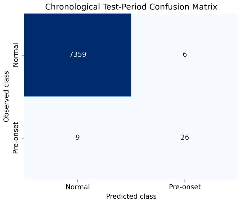
At the conventional 0.50 threshold, the chronological-test confusion matrix is [[7359, 6], [9, 26]], containing all 7400 untouched test windows. The six false alerts correspond to 1.54 false alerts per rotor-hour, or approximately one false alert every 39 min.
4.8. SHAP Analysis and Model Identity
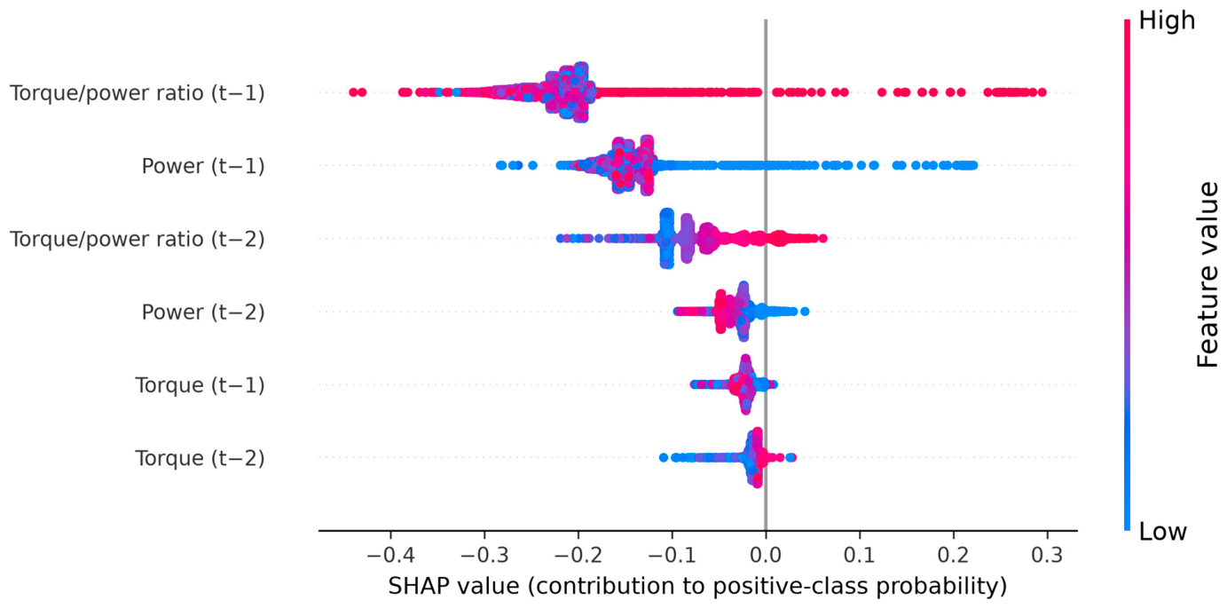
SHAP values are recomputed for the frozen Random Forest using TreeExplainer and the chronological test period. The positive-class output is selected explicitly, the resulting array is verified against the six-feature input matrix, and probability additivity is confirmed before plotting.
Mean absolute SHAP attribution ranks torque/power at t − 1 first (0.2193), followed by power at t − 1 (0.1459) and torque/power at t − 2 (0.0720). Rotor speed is not an input to this classifier. SHAP is interpreted as an explanation of model behaviour rather than evidence of physical causality.
4.9. Observational Multiplier Analysis
For the field comparison, free-spin is defined using the operational criterion:
A free-spin event is counted when a rotor transitions into this state. Counts are normalized by rotor operating time, with exact Poisson confidence intervals; incidence-rate ratios use an exact conditional Poisson interval. Recorded instantaneous electrical power is calculated as |−V_in I_in|, and uncertainty in mean instantaneous power is evaluated using five-minute rotor blocks.
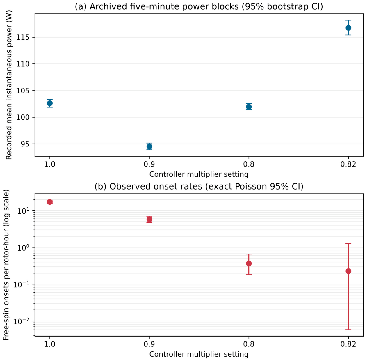
The archived all-row recorded mean instantaneous single-rotor power outputs are 101.95 W at setting 0.8, 94.57 W at 0.9, 102.67 W at 1.0, and 116.66 W at 0.82. The 0.82 excerpt is therefore 13.63% above the 1.0 excerpt. Analysis of five-minute blocks gives a closely aligned comparison of 13.76%, with a bootstrap 95% interval of 12.24–15.38%. This is an observational comparison of archived field excerpts, not a flow-normalized estimate of energy-production improvement.
The original three-anchor regression assessment produced identical candidate predictions for 0.75, 0.78, and 0.82. It therefore identifies a low-multiplier candidate region but does not establish a unique mathematical optimum.
Within the engineering development process, 0.82 was selected as the practical operating point after considering the recorded multiplier behaviour and operational response, and it was subsequently deployed. It is therefore described as an engineering-selected configuration rather than a universal optimum.
The 1.0 excerpt contains 337 free-spin onsets in 19.49 rotor-hours (17.29 events per rotor-hour), while the 0.82 excerpt contains one onset in 4.40 rotor-hours (0.23 events per rotor-hour). The observed incidence-rate ratio for 1.0 versus 0.82 is 76.1, with an exact conditional Poisson 95% CI of 13.6–3014.1. This is described as an observed free-spin onset-rate difference in the archived field excerpts, not as a general system-wide reliability reduction. The estimate remains uncertain because the 0.82 excerpt contains only one event.
4.10. Boundary of Demonstrated Integration
The demonstrated workflow comprises chronological onset classification, model comparison, SHAP-based interpretation, and observational controller-setting assessment. The study does not claim automatic classifier-to-controller actuation or a universally optimal multiplier.
5. Results
Random Forest showed strong discrimination on the untouched chronological test period, which contains 35 positive onsets and 7365 normal-operation windows. ROC-AUC was 98.3%, PR-AUC was 81.4%, and precision was 81.2% at the conventional 0.50 threshold. Sensitivity was 74.3% and F1 score was 77.6%, with a confusion matrix [[7359, 6], [9, 26]] across all 7400 test windows. These values replace the preliminary shuffled-window result as the primary predictive evaluation.
The six-feature SHAP analysis identifies torque/power at t − 1 as the strongest global model attribution, followed by power at t − 1 and torque/power at t − 2.
Figure 2 shows the distribution and direction of feature contributions across the chronological test observations. The result supports the interpretation that the most recent relationship between applied torque and generated power contains important information before a power-lapse onset.
Each positive example contains observations at t − 2 and t − 1 before an exact-zero-power onset at t. At the observed per-rotor sampling interval, this history spans approximately 1.25 s and the most recent input is approximately 0.624 s before the onset. This is the label geometry used for training; an online controller-response experiment was not demonstrated.
Thresholds were selected using the validation period. Logistic Regression had the strongest ranking metrics. The paired five-minute-block bootstrap difference in PR-AUC (Logistic Regression minus Random Forest) was 2.21 percentage points (95% CI −1.71 to 5.74), which includes zero. Random Forest is retained as the focal nonlinear model for continuity with the original analysis architecture and TreeSHAP interpretation.
Figure 3 presents the Random Forest confusion matrix on the chronological test period.
Observational MPPT Multiplier Comparison
The archived controller-setting excerpts show a low-multiplier operating region associated with fewer observed free-spin onsets. Recorded mean instantaneous power at 0.82 was 13.6% higher than in the prior 1.0 excerpt. The 0.8 excerpt exhibited a similarly low onset rate but did not show the same recorded mean instantaneous power, supporting an informed selection of an operating compromise rather than minimization of one outcome alone.
In the archived field excerpts, the selected 0.82 setting was associated with 13.6% higher recorded mean instantaneous power than the prior 1.0 configuration. The observed free-spin onset rate was approximately 76-fold lower at 0.82 than at 1.0 (0.23 versus 17.29 events per rotor-hour; incidence-rate ratio 76.1, exact conditional Poisson 95% CI 13.6–3014.1). This observational estimate remains uncertain because only one event occurred during the 4.40 rotor-hours recorded at 0.82, and the excerpts were not normalized to a flow velocity or matched to a duration.
Table 4 summarizes these observational comparisons.
It should be noted that the power intervals are bootstrap 95% confidence intervals for the mean of archived five-minute rotor blocks. Event-rate intervals are exact Poisson (Garwood) intervals, while incidence-rate-ratio intervals are exact conditional Poisson intervals.
Figure 4 shows the corresponding power and free-spin onset-rate comparisons, with onset rates presented on a logarithmic axis. Recorded onset counts/exposures were 337/19.49 rotor-hours at 1.0, 104/18.03 at 0.9, 11/30.15 at 0.8, and 1/4.40 at 0.82. The single observed onset in the 0.82 excerpt results in a wide confidence interval. The excerpts were recorded during different operating periods, were not duration-matched, and were not normalized for flow velocity, discharge, or water level.
6. Discussion
The prediction and controller-setting analyses complement each other. The classifier provides an interpretable short-horizon warning signal for power-lapse onset, while the field analysis identifies an operating configuration associated with higher recorded mean instantaneous power and fewer observed free-spin onsets in archived field excerpts. Together, they show how operational telemetry can support condition awareness and controller development on a distributed hydrokinetic system without establishing automatic actuation or a causal hydrodynamic effect.
The chronological experiment provides a more realistic assessment than a shuffled-window split. Logistic Regression achieved the strongest ranking metrics (ROC-AUC 99.8%, PR-AUC 83.6%), compared with Random Forest (98.3% and 81.4%). The paired five-minute-block bootstrap estimate for the PR-AUC difference was 2.21 percentage points (95% CI −1.71 to 5.74), so this dataset did not statistically resolve the observed ranking difference.
Random Forest remains the focal nonlinear model for continuity with the original architecture and TreeSHAP analysis. At the conventional 0.50 threshold, its 1.54 false alerts per rotor-hour correspond to approximately one false alert every 39 min. This may be acceptable for passive monitoring, but acceptability for automatic controller intervention has not been demonstrated; automatic classifier-triggered actuation is not included here.
This study uses a representative operational case study involving a hydrokinetic system with two rotor channels to demonstrate the practical application of an AI-supported decision-making framework for renewable energy systems. The analysis draws on 36,636 non-overlapping telemetry windows, including 279 independent positive episode onsets, with 35 occurring in the final chronological test period. The evaluation focuses on a specific operational dataset to illustrate how short-horizon event prediction, SHAP-based model interpretation, and field-informed controller optimization can be combined within a single framework.
The controller-setting analysis further demonstrates the practical application of this approach using recorded operational data, including the engineering-selected 0.82 configuration. While the field comparisons are observational and further validation across different operating conditions, devices, and sites would extend the findings, the results provide a practical demonstration of how operational telemetry and explainable AI can support condition monitoring and power-control optimization. The study therefore serves as an application-oriented example of the potential of AI-supported operational decision-making in hydrokinetic energy systems, providing a foundation for broader implementation and further development across distributed renewable energy applications.
7. Conclusions and Future Work
This study demonstrates the practical application of an AI-supported decision-making framework that combines short-horizon prediction of exact-zero-power onset, explainable machine learning, and field-informed power-control optimization in a distributed hydrokinetic energy system. Using operational telemetry from a hydrokinetic case study, the Random Forest classifier achieved a ROC-AUC of 98.3%, PR-AUC of 81.4%, and precision of 81.2% under chronological evaluation. SHAP analysis identified the torque-to-power ratio at t−1 as the leading model attribution, illustrating how explainable AI can provide insight into the operational parameters influencing model predictions and support data-driven condition monitoring.
The field evaluation further illustrates the potential of integrating predictive monitoring with operational power-control optimization. The selected 0.82 controller configuration was associated with 13.6% higher recorded mean instantaneous power compared with the prior 1.0 configuration, alongside an approximately 76-fold lower observed free-spin onset rate (0.23 versus 17.29 events per rotor-hour). These results represent an observational comparison of archived operating periods and demonstrate how field telemetry can inform controller-parameter selection. Together, the predictive and operational analyses provide a practical example of how AI-supported decision-making can contribute to improved operational awareness and the development of power-optimization strategies for renewable energy technologies such as hydrokinetic energy systems.
The primary contribution of this study lies in demonstrating how established machine-learning techniques, SHAP-based model interpretation, and field-informed control-parameter evaluation can be integrated into a practical framework for renewable energy applications. Using a specific hydrokinetic operating scenario as a case study, the proposed approach illustrates the potential of explainable AI to support the identification of operational anomalies, interpretation of model predictions, and development of data-driven control strategies.
Future work will focus on extending the framework to additional hydrokinetic devices and operating conditions, incorporating hydrodynamic measurements into controller-parameter evaluation, and investigating the integration of predictive model outputs into automated controller responses. These developments will support the continued advancement of AI-enabled operational decision-making for distributed hydrokinetic fleets, with potential applicability to other renewable energy systems.
Conference Paper: An earlier version of this work was published in the Proceedings of the 14th European Conference on Renewable Energy Systems (ECRES 2026), London, UK, 7–9 July 2026. The present manuscript is a substantially extended and revised version of that work [
29].
Author Contributions
Conceptualization, S.D. and C.M.N.; methodology, S.D.; software, S.D.; validation, S.D.; formal analysis, S.D.; investigation, S.D.; data curation, S.D.; visualization, S.D.; writing—original draft preparation, S.D. and C.M.N.; writing—review and editing, S.D. and C.M.N.; supervision and guidance on manuscript structure and academic presentation, C.M.N. All authors have read and agreed to the published version of the manuscript.
Funding
This research received no external funding. The study was conducted as part of an internal research and development project at Energyminer GmbH.
Data Availability Statement
Operational telemetry originated from a commercial field system and contains proprietary and confidential information. The data are therefore not publicly available. Aggregated or suitably anonymized supporting information may be made available by the corresponding author upon reasonable request, subject to commercial-confidentiality, intellectual-property, and data-governance restrictions.
Acknowledgments
The authors thank the Energyminer GmbH engineering team for field deployment and telemetry support, and the Technical University of Munich for supervision of the underlying master’s thesis from which this work is derived. The authors thank Andrea Stocco for his supervision.
Conflicts of Interest
The authors are affiliated with Energyminer GmbH, whose technology is examined in this study. The work relates to company technology and associated patent activity. These relationships are disclosed as potential conflicts of interest.
Nomenclature
| MPPT | Maximum power point tracking |
| PdM | Predictive maintenance |
| SCADA | Supervisory control and data acquisition |
| SHAP | Shapley additive explanations |
References
- Khan, M.J.; Bhuyan, G.; Iqbal, M.T.; Quaicoe, J.E. Hydrokinetic energy conversion systems and assessment of horizontal and vertical axis turbines for river and tidal applications: A technology status review. Appl. Energy 2009, 86, 1823–1835. [Google Scholar] [CrossRef] [Scilit]
- Chen, H.; Tang, T.; Aït-Ahmed, N.; Benbouzid, M.E.H.; Machmoum, M.; Zaïm, M.E.H. Attraction, challenge and current status of marine current energy. IEEE Access 2018, 6, 12665–12685. [Google Scholar] [CrossRef] [Scilit]
- Chica, E.; Velásquez, L.; Rubio-Clemente, A. Full-Scale Experimental Assessment of a Horizontal-Axis Hydrokinetic Turbine for River Applications: A Challenge for Developing Countries. Energies 2025, 18, 1657. [Google Scholar] [CrossRef] [Scilit]
- Stanilov, A.; Sharkov, R.; Alexandrov, A.; Velichkova, R.; Simova, I. Experimental Study of the Efficiency of Hydrokinetic Turbines Under Real River Conditions. Energies 2025, 18, 5160. [Google Scholar] [CrossRef] [Scilit]
- Canbay, Y.; Akay, O.E. Integrated deep learning models to predict future vibrations on the discharge ring of a river-type hydroelectric power plant. Meas. Sci. Technol. 2025, 36, 036150. [Google Scholar] [CrossRef] [Scilit]
- Randall, R.B. Vibration-Based Condition Monitoring: Industrial, Aerospace and Automotive Applications; Wiley: Chichester, UK, 2011. [Google Scholar]
- Feng, Y.; Qiu, Y.; Crabtree, C.J.; Long, H.; Tavner, P.J. Monitoring wind turbine gearboxes. Wind Energy 2013, 16, 728–740. [Google Scholar] [CrossRef] [Scilit]
- Kusiak, A.; Verma, A. A data-driven approach for monitoring blade pitch faults in wind turbines. IEEE Trans. Sustain. Energy 2011, 2, 87–96. [Google Scholar] [CrossRef] [Scilit]
- Schlechtingen, M.; Santos, I.F. Comparative analysis of neural network and regression based condition monitoring approaches for wind turbine fault detection. Mech. Syst. Signal Process. 2011, 25, 1849–1875. [Google Scholar] [CrossRef] [Scilit]
- Tchakoua, P.; Wamkeue, R.; Ouhrouche, M.; Slaoui-Hasnaoui, F.; Tameghe, T.A.; Ekemb, G. Wind turbine condition monitoring: State-of-the-art review, new trends, and future challenges. Energies 2014, 7, 2595–2630. [Google Scholar] [CrossRef] [Scilit]
- Stetco, A.; Dinmohammadi, F.; Zhao, X.; Robu, V.; Flynn, D.; Barnes, M.; Keane, J.; Nenadic, G. Machine learning methods for wind turbine condition monitoring: A review. Renew. Energy 2019, 133, 620–635. [Google Scholar] [CrossRef] [Scilit]
- Polagye, B.; Strom, B.; Ross, H.; Forbush, D.; Cavagnaro, R.J. Comparison of cross-flow turbine performance under torque-regulated and speed-regulated control. J. Renew. Sustain. Energy 2019, 11, 044501. [Google Scholar] [CrossRef] [Scilit]
- Garay, C.E.; Miranda Bonomi, F.A.; Mansilla, G.N.; Fagre, M.; Guzmán, S.G.; Ritorto, P.A.; Perez, F.I.; Katz, M. A Multimodal TinyML-Based Predictive Maintenance Architecture for Industrial IoT in the 6G Era. Sensors 2026, 26, 4536. [Google Scholar] [CrossRef] [Scilit]
- Breiman, L. Random forests. Mach. Learn. 2001, 45, 5–32. [Google Scholar] [CrossRef] [Scilit]
- Lundberg, S.M.; Lee, S.I. A unified approach to interpreting model predictions. In Proceedings of the 31st International Conference on Neural Information Processing Systems (NIPS 2017), Long Beach, CA, USA, 4–9 December 2017; Curran Associates: Red Hook, NY, USA, 2017; pp. 4765–4774. [Google Scholar]
- Lundberg, S.M.; Erion, G.; Chen, H.; DeGrave, A.; Prutkin, J.M.; Nair, B.; Katz, R.; Himmelfarb, J.; Bansal, N.; Lee, S.I. From local explanations to global understanding with explainable AI for trees. Nat. Mach. Intell. 2020, 2, 56–67. [Google Scholar] [CrossRef] [Scilit]
- Tang, Y.; VanZwieten, J.; Dunlap, B.; Wilson, D.; Sultan, C.; Xiros, N. In-Stream Hydrokinetic Turbine Fault Detection and Fault Tolerant Control—A Benchmark Model. In Proceedings of the 2019 American Control Conference, Philadelphia, PA, USA, 10–12 July 2019; pp. 4442–4447. [Google Scholar]
- Allmark, M.; Prickett, P.; Grosvenor, R. Detection of Tidal Stream Turbine Rotor Imbalance Faults for Turbulent Flow Conditions and Optimal Tip-Speed-Ratio Control. In Proceedings of the 12th European Wave and Tidal Energy Conference, Cork, Ireland, 27 August–1 September 2017. [Google Scholar]
- Chihaia, R.-A.; Vasile, I.; Cîrciumaru, G.; Nicolaie, S.; Tudor, E.; Dumitru, C. Improving the Energy Conversion Efficiency for Hydrokinetic Turbines Using MPPT Controller. Appl. Sci. 2020, 10, 7560. [Google Scholar] [CrossRef] [Scilit]
- Miladinović, N.; Kilibarda, F.; Radoman, U.; Polužanski, V.; Radovanović, V. Predictive Maintenance of Hydro Turbine-Generator Units: A Review. Appl. Sci. 2026, 16, 8607. [Google Scholar] [CrossRef] [Scilit]
- Betti, A.; Crisostomi, E.; Paolinelli, G.; Piazzi, A.; Ruffini, F.; Tucci, M. Condition monitoring and predictive maintenance methodologies for hydropower plants equipment. Renew. Energy 2021, 171, 246–253. [Google Scholar] [CrossRef] [Scilit]
- Hajimohammadali, F.; Crisostomi, E.; Tucci, M.; Fontana, N. Evaluating Deep Learning Networks Versus Hybrid Network for Smart Monitoring of Hydropower Plants. Energies 2024, 17, 5670. [Google Scholar] [CrossRef] [Scilit]
- Özcan, E.; Gür, S.; Eren, T. A Hybrid Model to Optimize the Maintenance Policies in the Hydroelectric Power Plants. J. Polytech. 2021, 24, 75–86. [Google Scholar] [CrossRef] [Scilit]
- Cerqueira, V.; Torgo, L.; Mozetič, I. Evaluating time series forecasting models: An empirical study on performance estimation methods. Mach. Learn. 2020, 109, 1997–2028. [Google Scholar] [CrossRef] [Scilit]
- Alnahhal, M.; Tabash, M.I.; Safi, S.K.; Al-Absy, M.S.M.; Mamadiyarov, Z. A Comparative Study of Imbalance-Handling Methods in Multiclass Predictive Maintenance. Computation 2026, 14, 88. [Google Scholar] [CrossRef] [Scilit]
- Sabanci, K.; Balci, S.; Aslan, M.F. Estimation of the switching losses in DC-DC boost converters by various machine learning methods. J. Energy Syst. 2020, 4, 1–11. [Google Scholar] [CrossRef] [Scilit]
- Chen, T.; Guestrin, C. XGBoost: A scalable tree boosting system. In Proceedings of the 22nd ACM SIGKDD International Conference on Knowledge Discovery and Data Mining (KDD 2016), San Francisco, CA, USA, 13–17 August 2016; ACM: New York, NY, USA, 2016; pp. 785–794. [Google Scholar]
- Rudin, C. Stop explaining black box machine learning models for high stakes decisions and use interpretable models instead. Nat. Mach. Intell. 2019, 1, 206–215. [Google Scholar] [CrossRef] [Scilit]
- Dalkiran, S.; Niebuhr, C.M. AI-Driven Predictive Maintenance and Power Optimization Strategy for Distributed Hydropower Systems. In Proceedings of the 14th European Conference on Renewable Energy Systems (ECRES 2026), London, UK, 7–9 July 2026. [Google Scholar]
| Disclaimer/Publisher’s Note: The statements, opinions and data contained in all publications are solely those of the individual author(s) and contributor(s) and not of MDPI and/or the editor(s). MDPI and/or the editor(s) disclaim responsibility for any injury to people or property resulting from any ideas, methods, instructions or products referred to in the content. |