Article

Bridging the Gap Between MP-PIC CPFD Hydrodynamic Simulations and CREC-GS-Optiprobes Data in a Sand Fluidized Bed for Biomass Gasification


by
Marcos Navarro Salazar
,
Nicolas Torres Brauer
and
Hugo de Lasa
*
Chemical Reactor Engineering Centre (CREC), Department of Chemical and Biochemical Engineering, Faculty of Engineering Science, Western University, London, ON N6A 5B9, Canada
*
Author to whom correspondence should be addressed.
Processes 2026, 14(18), 3002; https://doi.org/10.3390/pr14183002 (registering DOI)
Submission received: 15 July 2026 / Revised: 8 September 2026 / Accepted: 15 September 2026 / Published: 20 September 2026

Abstract

This study examines a sand bubbling fluidized bed containing cylindrical biomass pellets. It demonstrates the advantages of integrating fiber-optic measurements—such as those obtained with CREC-GS-Optiprobes—with CPFD Barracuda VR® 25.0.1 computational modeling. Experimental data collected by using CREC fiber-optic probes in a 43.8 cm diameter, laboratory-scale cold gasifier unit are used to validate the radial phase distributions predicted by CPFD Barracuda VR® simulations for the gas, emulsion, and biomass pellet phases. In addition, it is shown that the bubble rise velocity measurements provided by the CREC probes offer complementary insights into the limitations of CPFD Barracuda VR® simulations. These measurements highlight the importance of bubble–bubble interactions, including the “push” exerted by neighboring bubbles on a target bubble. Based on this approach, a combined experimental–computational methodology is proposed, leading to the development of a bubble rise velocity equation. This equation is expressed as a function of the isolated bubble’s axial chord and as a function of the superficial gas velocity in excess present at minimum fluidization conditions. It is anticipated that this equation will be beneficial for the design and optimization of sand fluidized bed gasifiers operating with biomass pellets, particularly by improving the prediction and capture of bubble dynamics.

1. Introduction

Today, the production of energy is one of the most critical global challenges given that it is intrinsically linked to economic development, social progress, and environmental sustainability. Global energy demand continues to rise alongside population growth and industrial expansion and is projected to increase by approximately 44%, by 2030 [1].
At present, fossil fuels are the dominant source of energy, accounting for more than 75% of global energy production [2]. Their combustion is the primary source of greenhouse gas emissions, particularly carbon dioxide (CO2), which significantly contributes to global warming and climate change [2]. Moreover, fossil fuels are finite, non-renewable resources, and thus, raise concerns about long-term energy security. These environmental and resource-related challenges have intensified the search for alternative and sustainable energy technologies.
Among renewable resources, biomass has emerged as a promising candidate due to its widespread availability and its potential to produce near carbon-neutral energy. Thermochemical conversion processes, particularly gasification, enable the transformation of biomass into synthesis gas (syngas), which is a versatile mixture primarily composed of CO, H2, CO2, and CH4 [3]. Syngas can be used directly for heat and power generation or can be further upgraded into value-added fuels and chemicals [4]. Fluidized bed gasifiers are especially attractive for biomass conversion because they provide excellent gas–solid contact, enhanced heat and mass transfer, and relatively uniform temperature distributions, all of which promote efficient and stable operation [5,6,7].
Despite these advantages, the hydrodynamic behavior of fluidized beds is inherently complex, involving factors such as multiphase interactions, bubble formation, particle clustering, the circulation of solids, and transient flow structures [8]. These phenomena strongly influence reactor performance, conversion efficiency, and product distribution. These characteristics need to be assessed to address significant challenges in reactor design, optimization, and scale-up. Consequently, predictive tools capable of accurately describing gas–solid flow dynamics, such as the CREC-GS-Optiprobes, are essential.
The present work is built upon previously reported experimental hydrodynamic measurements obtained through our team’s use of the CREC-GS-Optiprobe system in 2026 [8]. This study enabled the high-resolution characterization of gas–solid flow behavior in a biomass fluidized bed reactor loaded with cylindrical biomass pellets. This experimental dataset was compared in the present study, with computational particle fluid dynamic (CPFD) simulations conducted using Barracuda VR®, while employing the multiphase particle-in-cell (MP-PIC) methodology. This comparison allowed a rigorous assessment of the predictive capabilities and limitations of CPFD Barracuda VR® model in sand fluidized beds loaded with cylindrical biomass pellets. This allows us to establish a new bubble rising velocity equation based on bubble axial chord and gas excess velocity, applicable to medium pressure biomass gasifiers (Appendix A). It is our view that the original reported results support reactor design, optimization, and scale-up of thermochemical biomass conversion processes.

2. Fluidized Bed Simulation

Computational particle fluid dynamics (CPFD) has become a powerful tool for analyzing multiphase systems and investigating fluidization behavior under a wide range of operating conditions [9,10,11,12]. In this study, all simulations were conducted using the CPFD Barracuda VR® software. Among the available numerical techniques, this software employs the multiphase particle-in-cell (MP-PIC) method for modeling dense gas–solid flows. The MP-PIC framework combines a Lagrangian treatment of particle parcels with a Eulerian description of the gas phase, enabling the simulation of large-scale fluidized bed units. This simulation has the advantage of being performed at a reasonable computational cost [13,14]. This hybrid approach effectively captures particle–particle interactions, solids stress effects, and heterogeneous flow structures, making it particularly well suited for the study of fluidized bed applications.

2.1. Governing Equations in CPFD-MP-PIC Modeling

To perform CPFD simulations by using the MP-PIC approach and to determine the hydrodynamics of a dense-phase sand fluidized bed, it is necessary to consider the following mass and momentum balance equations:

2.1.1. Fluid Phase

(a)
The continuity equation for gas phase [15]:
ρ f θ f t + · ρ f θ f u f = 0
where ρ f represents the fluid’s density, θf stands for the fluid’s volume fraction, t denotes the time and u f is the fluid’s velocity.
(b)
The momentum conservation equation for the fluid phase [15]:
ρ f θ f u f t + · ρ f θ f u f = p F + ρ f θ f g + θ f τ f
where ρf is the fluid’s density, p is the pressure, and g is the gravitational acceleration. The F function corresponds to the rate of momentum exchange between the fluid and the particle phase, and can be defined as:
F = f m p D p u f u p ρ ρ p + u p d m p d t d m p d u p d T P
where f represents the particle distribution function (PDF) (which is a function of the particle spatial location x p ), u p , stands for the particle velocity, mp denotes the particle mass, Tp represents the particle temperature, and t stands for the time. Furthermore, D p represents the drag force function, u f is the fluid velocity, ρ is the system pressure, and ρ p is the particle’s density.
Finally, the component of the stress τ f , for the “ij” indexes can be defined as:
F τ f , i j = μ u i x i + u j x j 2 3 μ δ i j u k x k
where μ is the shear viscosity, xi and xj represent the spatial computational volume locations at i and j respectively, and ui and uj stand for the component fluid velocities of the i and j elements, respectively.

2.1.2. Particle Phase

The dynamics of the particle phase are described by using the particle probability distribution function ϕ (x, up, ρp, Ωp, t), where x is the particle position, up is the particle velocity, ρ p is the particle density, Ωp is the particle volume and t is the time. It is further assumed that the mass of each particle remains constant over time, implying that there is no mass transfer between the particles and the fluid [15]. This assumption is appropriate for a cold gasifier simulator unit, with no gasification taking place.
The time evolution of ϕ is obtained by solving the Liouville equation for the particle distribution function (Equation (5)) as follows:
ϕ t + · ϕ u p + u p · ϕ A = 0
where u p is the divergence operator with respect to the particle velocity and A represents the discrete particle acceleration. A can be expressed as follows:
A = D p u f u p p ρ p + g τ θ p ρ p + u p ¯ u f τ D
where D p u f u p represents the acceleration due to the aerodynamic drag, p ρ p denotes the pressure gradient, g is the gravity, and τ θ p ρ p + u p ¯ u f τ D stands for the gradient of the interparticle stress [15,16].
Additionally, the drag force exerted on a particle by the fluid depends on the interphase drag coefficient, which can be expressed as:
D p = 3 8 ρ f u f u p ρ p r p C d
C d represents the drag coefficient calculated by using adequate drag models.
Regarding the particle-to-particle interactions, a model to evaluate the particle stress function was established, as described by Equation (8) [14,15]:
τ θ p = 10 P s θ p β m a x θ C P θ p ,     ε 1 θ p
where Ps corresponds to a pressure parameter, θ C P represents the close-packing particle volume fraction, and β is a factor of 2 to 5 [14,15,17] flow structures, making it particularly well suited for the study of fluidized bed applications.

2.2. Drag Models

In order to determine the drag coefficient (Cd), as described by Equation (7), an appropriate drag model must be selected. The chosen model should account for several particle-related parameters, including particle size distribution, particle shape, column geometry, and other relevant characteristics [13]. In the present study, two different drag models were employed to represent the particles involved in the fluidization process. Specifically, the Wen–Yu–Ergun model was used to represent the sand particles, while the non-spherical Haider–Levenspiel model was employed to stand for the cylindrical pellets.

2.2.1. Wen–Yu–Ergin Model

The Wen–Yu–Ergun model consists of a combination of two individual drag correlations: the Wen–Yu drag model [6], which is typically used to stand for fluid dilute-phase systems,
D 1 = 24 R e θ f 2.65 R e < 0.5 24 R e θ f 2.65   1 + 0.15 R e 0.687 0.5 R e 1000 0.44 θ f 2.65 R e > 1000
and the Ergun drag model [5], which is commonly employed to represent dense-phase fluidized conditions:
D 2 = 0.5 180 θ p θ f R e + 2 ρ f u f u p ρ p r p
Thus, the Wen–Yu–Ergun combined correlation provides accurate predictions for both low and high particle concentrations in fluidized beds, with Cd corresponding to a drag function parameter, ensuring reliable predictions, at intermediate concentrations. Parameter Cd is calculated as follows:
C d = D 1 θ p < 0.75 θ C P D 1 D 2 θ p 0.75 θ C P 0.85 θ C P 0.75 θ C P 0.75 θ C P θ p 0.85 θ C P D 2 θ p > 0.85 θ C P
where D 1 represents the Wen–Yu drag coefficient calculated with Equation (9) and D 2 corresponds to the Ergun drag coefficient obtained from Equation (10).

2.2.2. Non-Spherical Haider–Levenspiel Model

The Haider–Levenspiel drag model [18], developed for non-spherical particles, can be expressed as:
C d = 24 R e 1 + A R e B + C 1 + D R e
Equation (12) includes the parameters A, B, C, and D, which were determined by minimizing the root mean square error between the predicted and experimental drag coefficient values for various non-spherical particle geometries [18,19]. Collectively, these coefficients account for the contributions of the viscous and inertial drag components, enabling the correlation to accurately predict the drag coefficient over a broad range of Reynolds numbers. For non-spherical particles, it was demonstrated that these coefficients depend solely on the particle sphericity φ, in the range of 0.67 ≤ φ ≤ 0.906. As a result, the parameters A, B, C, and D were established as follows:
A = e x p 2.3288 6.4581 φ + 2.4486 φ 2
B = 0.0964 + 0.5565 φ
C = e x p 4.905 12.8944 φ + 18.42222 φ 2 10.2599 φ 3
D = e x p 1.4681 12.2584 φ + 20.7322 φ 2 15.8855 φ 3
By substituting the values obtained with Equations (13)–(16) into Equation (12), the following equation for the prediction of C d as a function of φ is obtained:
C d = 24 R e 1 + 8.1716   e x p 4.0655 φ × R e 0.0964 + 0.5565 φ + 73.69   R e   e x p 5.0748 φ R e + 5.378   e x p 6.2122 φ

3. Experimental Setup

3.1. Cold Gasifier Unit

In this present study, a cold gasifier model unit was studied to obtain its fluid-dynamic characteristics, as represented in (Figure 1). Figure 1 reports the various unit dimensions. It shows the position of the wind box, the air supply, the CREC fiber-optic probes, and the video camera and cyclone.
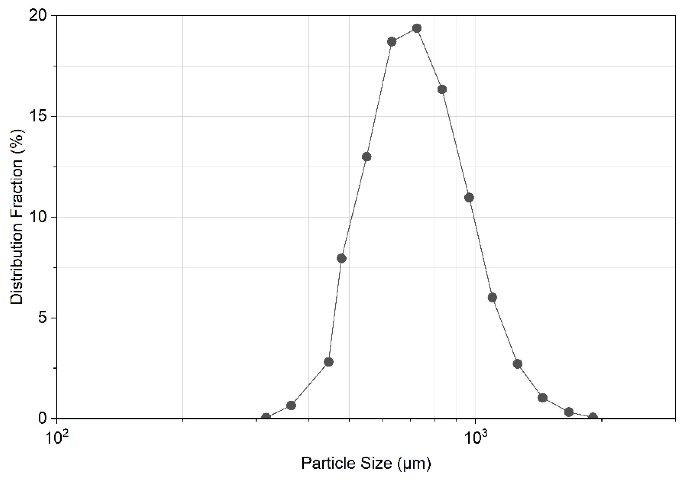
Additional details of the laboratory-scale sand fluidized bed unit are reported by Torres Breauer et al. [20]. The column is filled with silica sand (SiO2) particles having a particle size distribution (PSD) ranging from 320 to 1100 μm, and a mean diameter of 661 μm, as shown in Figure 2.
Furthermore, compressed air is introduced into the bed through a gas distributor plate. The cold gasifier unit is equipped with a camera located at the top of the upper section that is used to record the surface of the sand bed. In addition, the CREC-GS-Optiprobe system is employed to record both bubble axial chords (BAC) and bubble rise velocities (BRV). Finally, a cyclone separator is installed at the upper section of the gasifier in order to recirculate particles entrained during fluidization. Additional details regarding the CREC Optiprobes, their design, configuration, spacing and data treatment, in the fluidized bed unit are summarized in Appendix B and reported in Navarro Salazar et al. [8,21].

3.2. CREC-GS-Optiprobe System

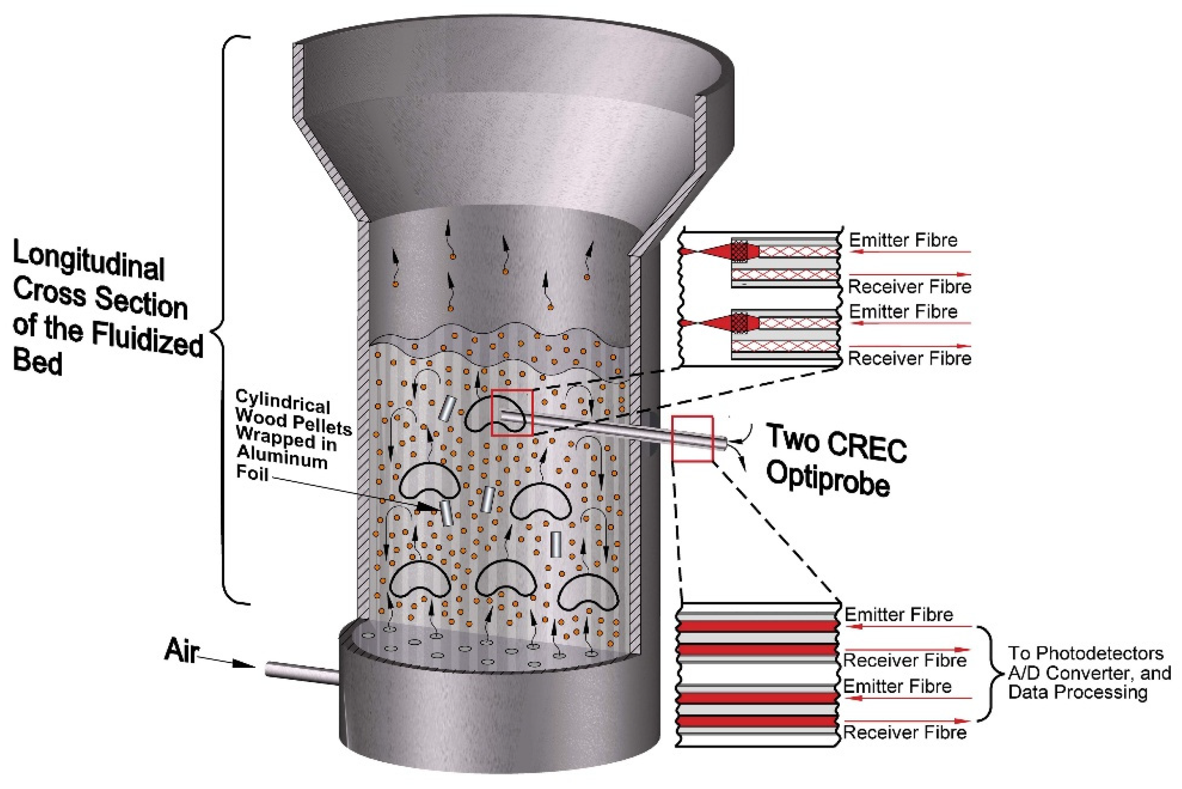
In the present study, bubbles formed in the fluidized bed are measured using a CREC-GS-Optiprobe system. This system is composed of 2 laser diodes, with a wavelength of 850 μm, and 2 optical fibers. One of the fibers is used to transmit a laser beam, while the other is employed to capture beam reflections, transmitting them to a photosensor. The potential effect of the miniaturized CREC-GS-Optiprobe sensors was analyzed in detail by Torres Brauer et al. [14] in a sand fluidized bed with a particle size distribution close to one used in the present study showing that the probe intrusion effect was negligible. A longitudinal cross-section of the fluidized bed reactor is presented in Figure 3.
The biomass feedstock consists of cylindrical wood pellets (as shown in Figure 3) with an average diameter of 0.79 cm and a length of 2.70 cm. The pellets are wrapped in aluminum foil to enhance signal detection by the CREC-GS-Optiprobe system, ensuring accurate tracking of particle motion during the fluidization experiments.

3.3. Simulation Setup

In this study, CPFD Barracuda VR® 25.0.1 was employed to simulate dense gas–solid systems due to its relatively lower computational cost compared to other numerical approaches, such as the discrete element method (DEM)-based models [22,23]. Simulation conditions are presented in Table 1. All simulations were performed using one of the Digital Research Alliance of Canada’s cluster called Nibi. On this cluster, a fraction of a node, consisting of 16 cores, 14 Gb of memory ram and one NVIDIA H100 SXM (80Gb) GPU was requested to perform calculations averaging 7 h of computation per run.
Furthermore, three different superficial air velocities were applied, as summarized in Table 2. These operating conditions were previously evaluated experimentally and used here for model validation.

3.4. Grid Analysis

CPFD Barracuda VR® employs structured grids to perform simulations. Therefore, selecting an appropriate grid resolution is essential to obtain reliable and accurate results. However, increasing the number of grid cells does not necessarily guarantee improved accuracy, as excessively fine meshes may lead to unnecessary computational cost without significantly enhancing the solution. For this reason, a grid independence analysis was conducted to determine the optimal mesh resolution.
Three different grid configurations were tested: (a) a coarse grid mesh consisting of 10,656 cells, with an average cell length and volume of 2.770 × 10⁻² m and 2.125 × 10⁻⁵ m3, respectively; (b) a medium mesh consisting of 87,040 cells, with an average cell length and volume of 1.410 × 10⁻² m and 2.803 × 10⁻⁶ m3, respectively; and (c) a fine mesh consisting of 664,020 cells, with an average cell length and volume of 0.710 × 10⁻² m and 3.578 × 10⁻⁷ m3, respectively. The influence of grid resolution was evaluated using global quantities, such as: (a) pressure drop and cross-sectionally averaged particle volume (PVF), (b) spatial profiles, such as radial distributions of PVF, and (c) transport quantities, such as fluid and particle mass fluxes. Table 3 summarizes the key hydrodynamic quantities obtained when using the three mesh resolutions considered in this study for a mass flow rate of 0.0405 kg/s, which corresponds to the medium value with respect to the three different conditions used in this research.
As shown in Table 3, the predicted pressure drops across the bed exhibit a clear agreement among the different grid configurations. The relative difference between various pressure drops predictions of the coarse and medium meshes is 7.03%, whereas the relative difference between the medium and fine meshes decreases to 1.61%. Given that the latter variation is small, it indicates a weak sensitivity of the pressure drop to further grid refinement, confirming that the medium mesh provides grid-independent results.
Furthermore, transport quantities using the three different mesh configurations were further analyzed by considering fluid and particle mass fluxes. The predicted fluid mass flux for all mesh configurations showed excellent numerical agreement, with variation of results between mesh configurations being below 1%, indicating that there is grid-independent fluid transport. The standard deviation of the particle mass flux was substantially higher for the coarse mesh (43.53 kg/sm2) compared with the medium (19.21 kg/sm2) and fine (11.08 kg/sm2) meshes, indicating smaller fluctuations in the predicted particle transport for the finer grids. Although the standard deviation decreased further from the medium to the fine mesh, the mean particle mass fluxes remained nearly identical, with values of 0.270 and 0.269 kg/sm2, respectively, corresponding to a relative difference of only 0.43%. This indicates that further refinement from the medium to the fine mesh with a much higher computational cost and a negligible effect on the predicted mean particle mass flux is not justified. As a result, the medium-size mesh of Table 3 was adopted for further computations.
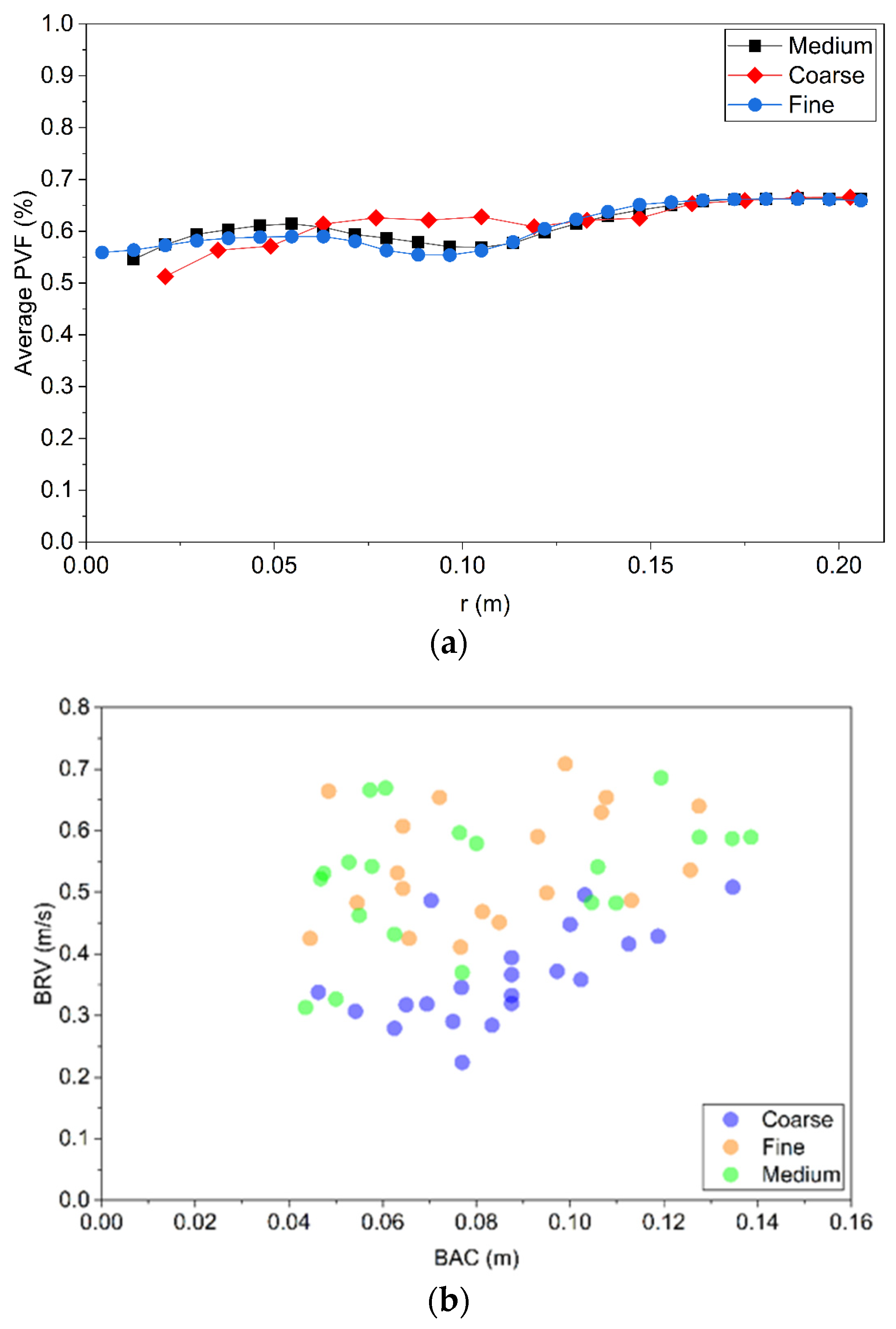
The grid dependence of solid holdup was evaluated by employing both cross-sectionally averaged PVF and radial PVF profiles. The average PVF showed augmenting monotonic convergence with increasing mesh resolution, with the relative difference between the medium and fine meshes being 0.96%. Radial PVF distributions obtained using the medium and fine meshes, as shown in Figure 4a, displayed close agreement across the reactor radius, particularly in the near-wall region. Slight deviations were observed in the bed core, which can be attributed to the inherently unsteady and heterogeneous nature of bubble-driven particle motion.
The grid analysis was also extended to the BRVs and BACs with the average data and standard deviation for the coarse, medium and fine case, as shown in Figure 4b, displaying the following results. (a) Coarse Grid: 0.364 m/s (±20.6%) and 0.086 m (±24.8%). (b) Medium Grid: 0.546 m/s (±16.8%) and 0.084 m (±37.7%). (c) Fine Grid: 0.526 m/s (±19.6%) and 0.080 m (±30.5%). This confirms as well that the medium grid was adequate for the CPFD Barracuda software simulation for the present study.
Overall, the results demonstrate that the medium mesh (87,040 cells) provides grid-independent predictions of the hydrodynamic and transport quantities while maintaining a reasonable computational cost. Consequently, this mesh resolution was selected for all subsequent simulations.

3.5. CPFD-Bubbles Detection

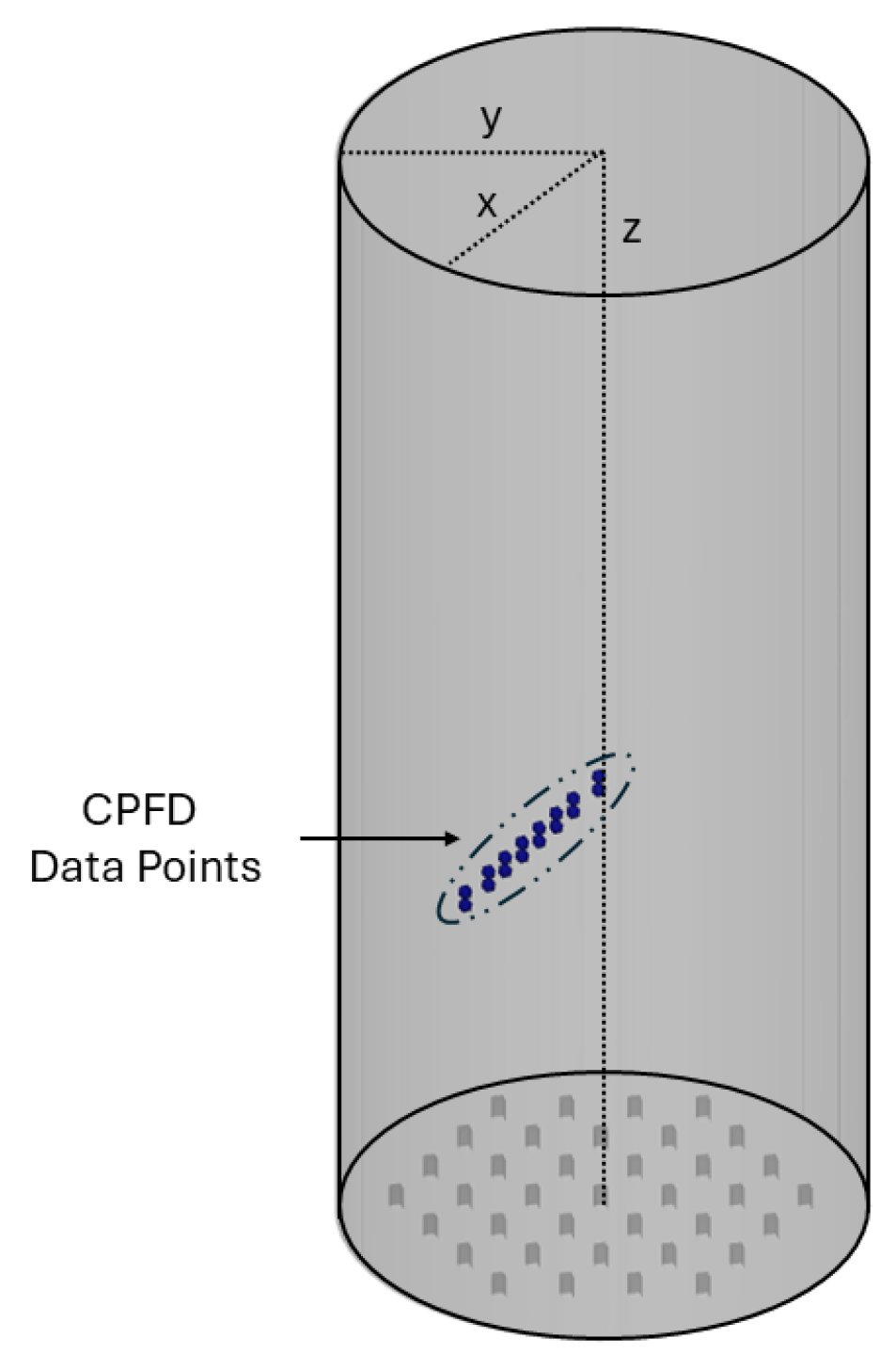
To identify computational bubbles, a set of “data point locations” was employed within the CPFD Barracuda VR® simulation domain, as illustrated in Figure 5. These data points act as virtual probes and use the exact measurement locations employed by the CREC-GS-Optiprobe system, including the same 0.40 m axial height and radial positions from r/R = 0 (center of the reactor) through r/R = 1 (reactor wall). This approach ensured that both experimental and computational bubbles were measured under equivalent sampling conditions, thereby providing a rigorous validation of the MP-PIC model predictions.
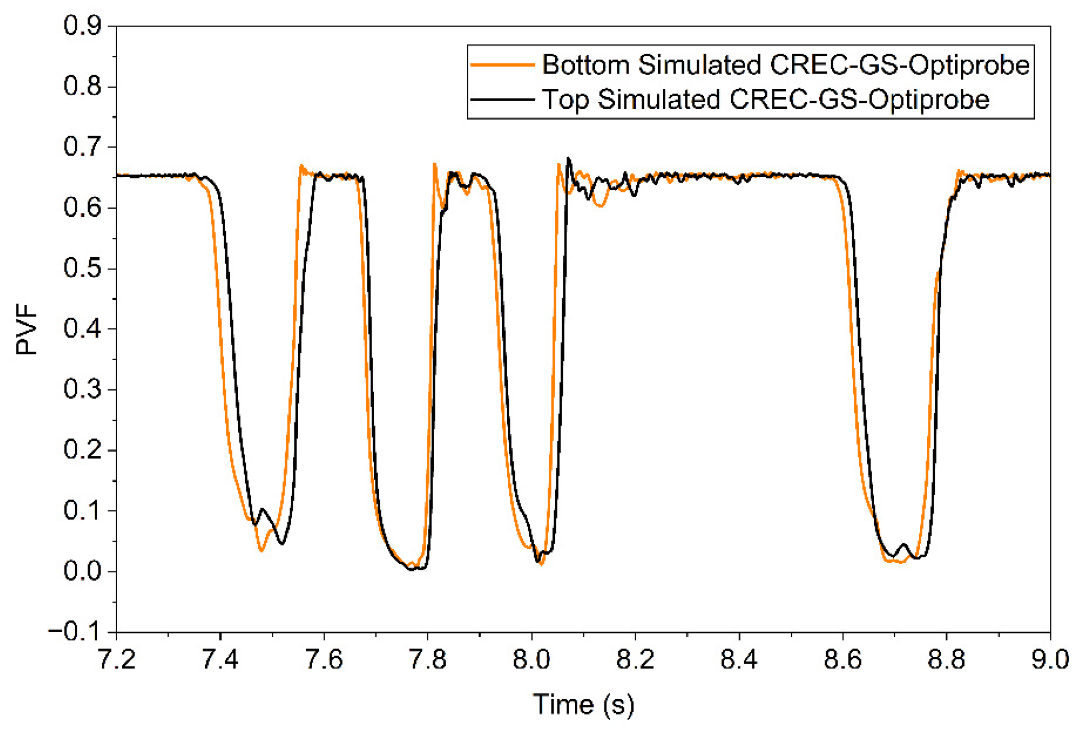
Furthermore, Figure 6 shows the characteristic computational signals obtained from the upper and lower virtual probes implemented in the CPFD model. The virtual probes emulate the operation of the CREC-GS-Optiprobe system by monitoring the local particle volume fractions at various radial locations. When a bubble passes through the sensing region, a decrease in sand particle concentration is detected, resulting in a corresponding drop in the simulated signal intensity. These signal fluctuations were processed using a MATLAB® R2024b script specifically developed for the CPFD data, while following the same fundamental data-processing criteria used for the experimental measurements, reported by Navarro Salazar et al. [8]. The particle volume fraction (PVF) was processed to identify bubble events and calculate the corresponding hydrodynamic parameters. In this treatment, signals with PVF values below 0.5 were identified as bubble events.

4. Results

The following section presents a comparison between the experimental measurements and the CPFD predictions obtained using the MP-PIC model with the CPFD Barracuda VR® software. The analysis was performed at superficial gas velocities of 0.250, 0.281, and 0.344 m/s and biomass loadings of 0 vol% and 2.5 vol%. Experimental and computational data were collected at identical measurement locations to ensure a direct and consistent comparison of the hydrodynamic parameters.

4.1. Hold up for the Gas, Pellet and Emulsion Phases

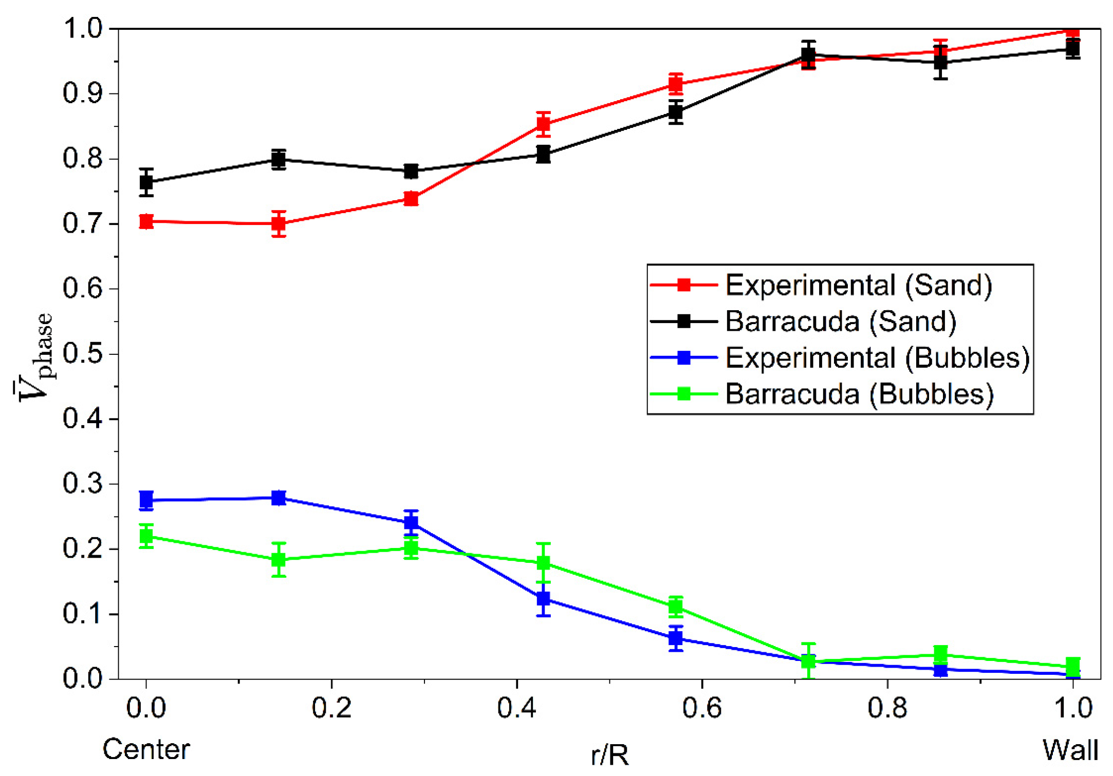
Experimental volumetric fractions for biomass, bubble and emulsion phases were obtained by following the methodology proposed by Navarro Salazar et al. [8]. These results were compared with the data obtained with CPFD simulations. These comparisons are presented in Figure 7 and Figure 8.
Figure 7 reports the radial distributions of the average sand and bubble volumetric fractions obtained experimentally and of those predicted by the MP-PIC model implemented in the CPFD software. It can be observed that the average sand volumetric fraction increased from the center of the reactor toward the wall, while the average bubble volumetric fraction exhibited the opposite trend. This behavior is characteristic of bubbling fluidized beds, where bubbles tend to concentrate near the reactor core, promoting a lower concentration of solids in the central region and a higher concentration of solids near the walls [3,4,5,6].
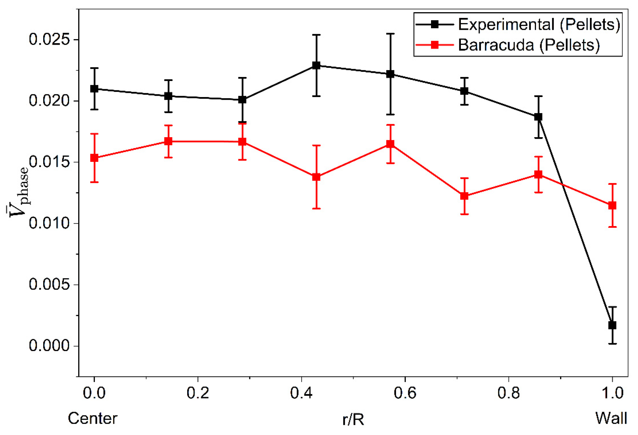
Figure 8 compares the radial distributions of the average biomass pellet volumetric fraction obtained experimentally and that acquired using CPFD simulations. Both datasets show a largely uniform pellet distribution across most of the bed cross-section, indicating that the biomass pellets remain well dispersed within the fluidized bed. The simulations also reproduce the overall magnitudes and spatial trends of the biomass pellet volumetric fractions reasonably well, although some discrepancies appear at the position of r/R = 1, being near to the reactor wall, where the experimental data exhibits a sharper decline in pellet concentration. These differences may stem from limitations in representing particle shape, particle–particle interactions, and/or local segregation effects within the MP PIC framework.

4.2. Bubble Rise Velocity and Bubble Axial Chord in a Sand Fluidized Bed

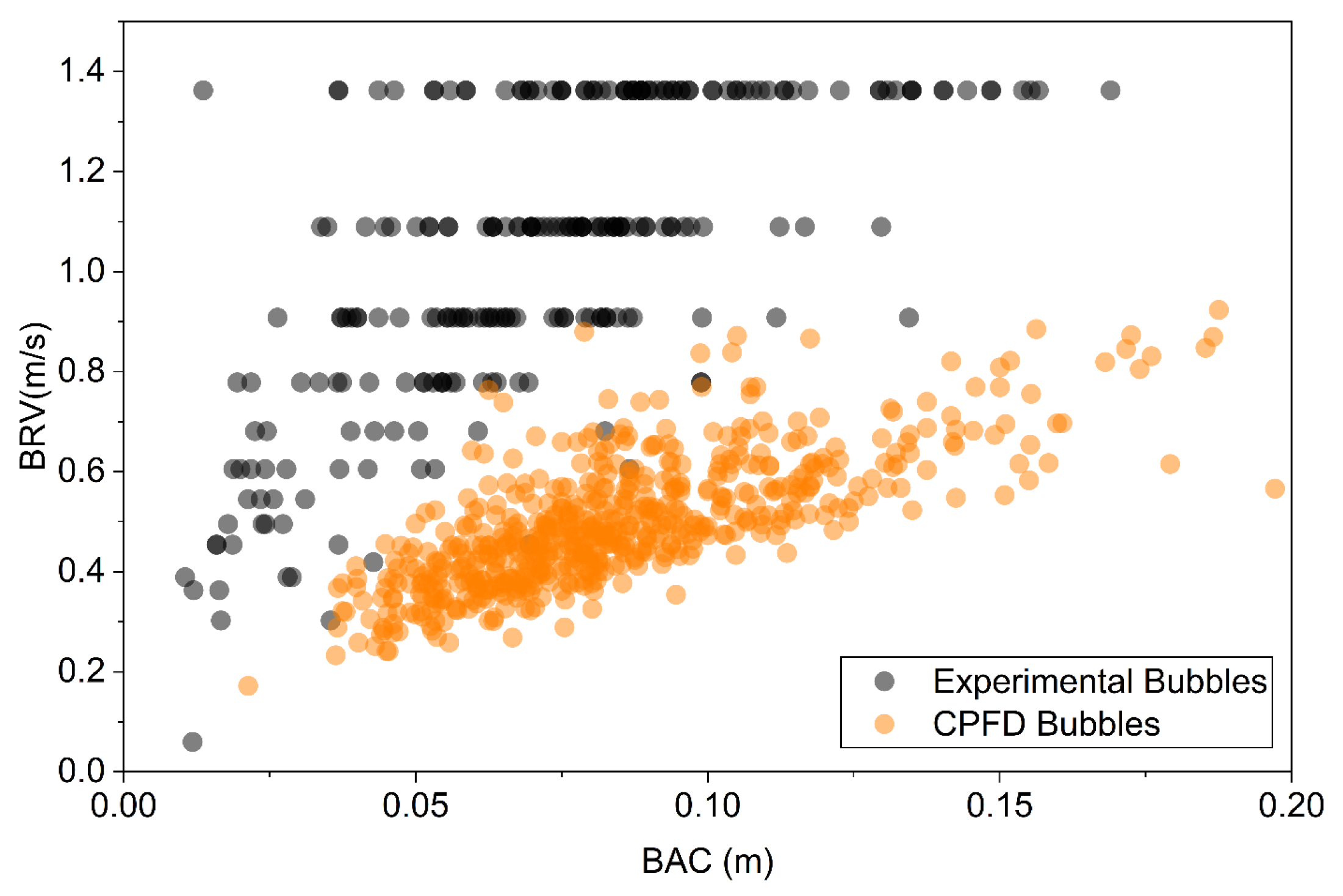
BRVs, BACs and their relationships as observed experimentally in the present study, and described in Section 3.2, were compared with BRV and BAC data acquired with CPFD Barracuda simulations, as shown in Figure 9. It was observed that bubble velocities plotted as a function of the diameter of the bubble ( D b ), and the bubble axial chord measured using the CREC-GS-Optiprobes, showed significant disagreement with that obtained with the CPFD bubble simulations. This discrepancy was consistent across all three superficial gas velocities evaluated.
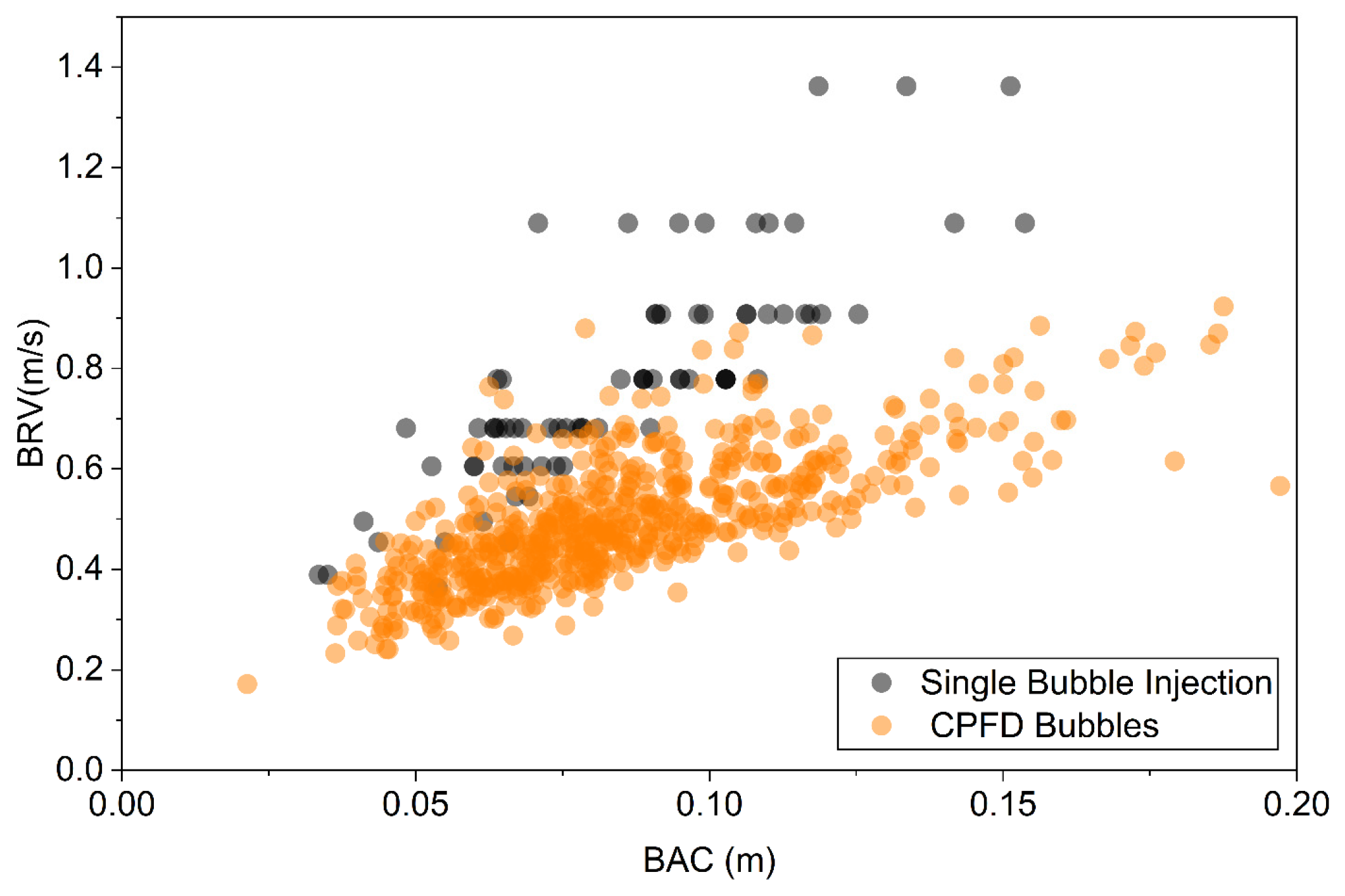
To help explain the observed disagreement, the CPFD Barracuda bubble dynamics simulation was compared with experimental data from a previous study by our research group (Torres Brauer et al. [14]), that used a similar sand fluidized bed where single bubbles were injected into a sand bed operating close to minimum fluidization ( υ a i r = 0.17   m s ) [14] as shown in Figure 10. These operating conditions and their related fluid dynamic parameters corresponding to 1.5 to 2 minimum superficial velocities were experimentally evaluated in Navarro Salazar et al. [8].
It can be observed from this figure that there is reasonable agreement between the CPFD Barracuda simulations and the single bubble dynamics reported in the reference study. This suggests that the CPFD Barracuda model tends to accurately predict the behavior of isolated bubbles but does not fully capture interactions among multiple bubbles coexisting within the bed. On this basis, Wherther’s modified bubble prediction model was applied, as it can fit experimental bubble data for A, B and D type powders of the Geldart classification [5,24,25], using the following equation:
υ b = α U U m f + γ g B A C
where α is a parameter that accounts for the differences between BRVs as a function of BACs in experiments and in CPFD simulations, U is the air velocity, U m f corresponds to the minimum fluidization air velocity, BAC accounts for the bubble diameter, g represents the gravity force, and γ is an empirical coefficient with a 0.5 value [26].
Following this approach, and to improve the adjustment of the BRV obtained in CPFD Barracuda with the experimental BRV results obtained from the CREC-GS-Optiprobe, the following equation is proposed:
B R V a d u j s t e d = α U U m f + B R V C P F D
where B R V C P F D represents the original value obtained from CPFD Barracuda before the adjustment.
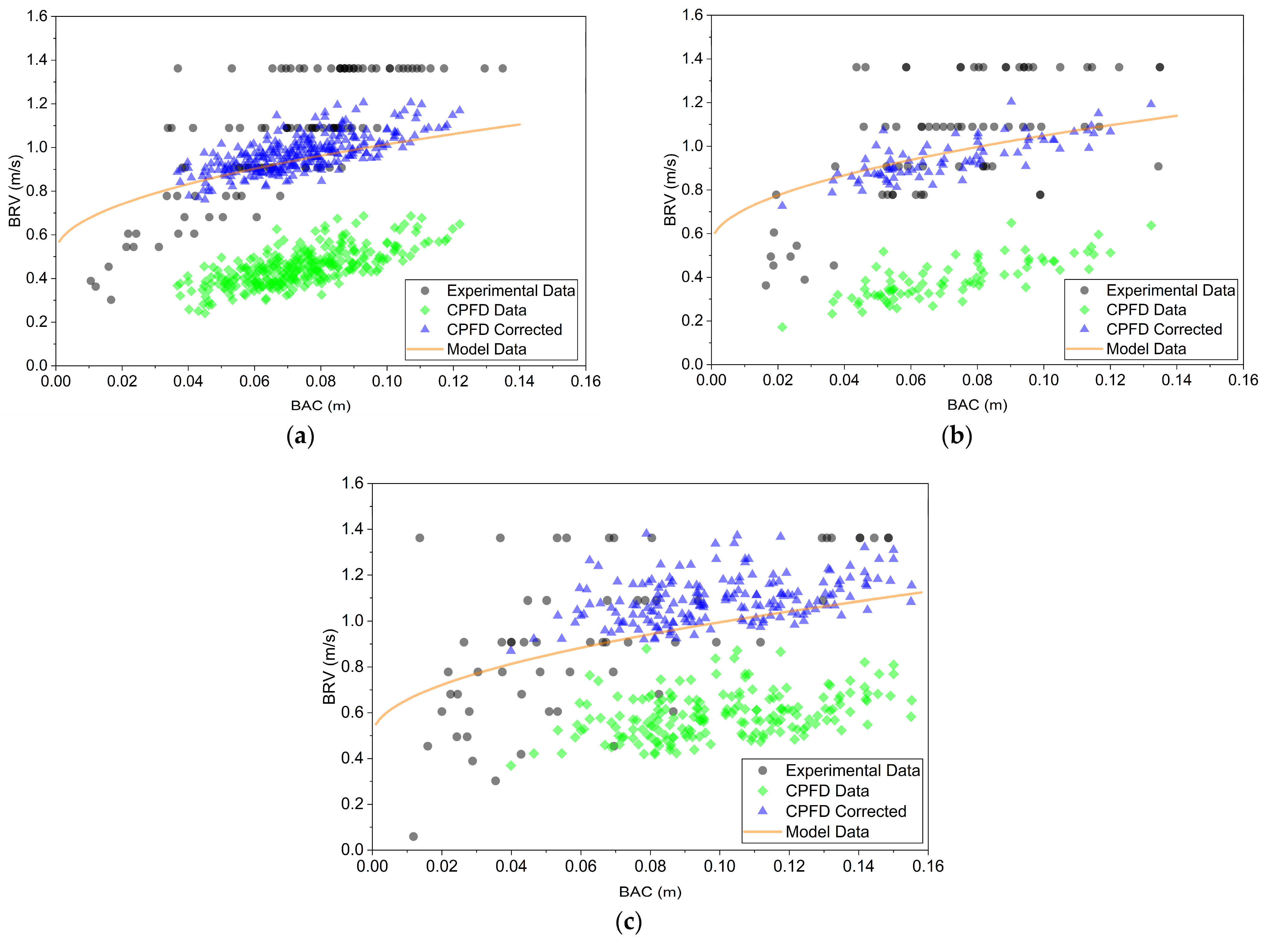
Figure 11a–c reports a comparison between the rising velocity of the bubble ( υ b ) obtained from Equation (18), the one acquired from the experimental data of the sand bubbling bed, the original CPFD Barracuda results and the B R V a d u j s t e d values obtained from Equation (19), for the three different air velocities tested, for superficial gas velocities corresponding to 1.5 to 2 Umf. One can notice the model data obtained from Equation (18), presents a good adjustment with the experimental results obtained from the CREC-GS-Optioprobes. On the other hand, the CPFD Barracuda predictions, before the correction from Equation (19), are below the predictions of the model and the experimental results.
Additionally, to quantitatively represent the applicability of the proposed model from Equation (19), Table 4 presents the comparisons of the Root Mean Square Error (RMSE) with respect to the experimental, CPFD and CPFD corrected data, and the different values of α used. The α parameter, as reported in Table 4, was calibrated as follows: (a) first, the experimental data from the CRECG-S-Optiprobes was employed to define the α term, and (b) in the next step, the Barracuda simulation was revised with the α (U-Umf) term to provide an independent confirmation of the suitability of the α variable.
As shown in Table 4, the α parameter decreases as the superficial gas velocity increases, with average α values being 6.49, 4.99, and 2.96 for 0.250, 0.281, and 0.344 m/s superficial gas velocities, respectively. In addition, the RMSE for the case of the comparisons of the experimental vs. Equation (18) results presented smaller errors despite the wide dispersion of the experimental data, as shown in Figure 11a–c. In contrast, the values for the RMSE for the case of the non-corrected CPFD vs. Equation (18) results show larger errors despite the low dispersion in the data cluster. Finally, it can also be noticed that once the CPFD is adjusted by using Equation (19), the error decreases considerably with respect to the original CPFD results, proving that the correction made by applying Equation (19) improves the adjust of the CPFD Barracuda results with respect to the experimental result obtained from the CREC-GS-Optiprobes. This trend suggests that the influence of the excess superficial gas velocity on BRVs becomes less pronounced at higher operating velocities, where bubble motion is increasingly governed by the bubble size term ( γ g B A C ), and by the enhanced gas–solid interactions associated with more vigorous fluidization.
Moreover, the variations in α also indicate a consistent increase on bubble rising velocity with BACs, suggesting a greater overall upward push exerted on individual bubbles, under these conditions. This phenomenon can be explained by the expected bubble deformation at higher BACs, which produces flatter bubbles with an increased backward-facing surface area per unit volume.
Previous studies have applied CPFD Barracuda VR® software, based on the MP-PIC approach, to simulate bubbling fluidized beds for Geldart particle classification of types A, B and D [14,27,28,29,30]. These studies reported discrepancies in the prediction of bubble rise velocity. Consequently, several model parameters were calibrated or optimized to improve the agreement between simulations and experiments.
Similarly, the present study identified systematic discrepancies between the experimentally measured and CPFD-predicted bubble rise velocities in a bubbling fluidized bed containing sand particles with a particle size distribution spanning the transition between Geldart B and D classifications. Based on this, an empirical correction parameter α was introduced to account for the hydrodynamic effects associated with bubble interactions that are not fully represented by the MP-PIC model. This correction significantly improves the agreement between the experimental measurements and the CPFD predictions without modifying the underlying numerical formulation of the Barracuda solver.
As a result, it can be concluded that in order to effectively use CPFD Barracuda simulation results to improve bubble rise velocity in bubbling sand fluidized beds, it is necessary to also account for the overall “push” exerted by surrounding bubbles on the bubble under consideration. Accurate evaluation of this collective “push” effect requires measurements obtained with the CREC-GS-Optiprobes such as those reported in the present study.

5. Conclusions

i.
The bubble rise velocity calculated using CPFD Barracuda VR® is in close agreement with the bubble rise velocity experimentally measured using the CREC-GS-Optiprobes for single injected bubbles in a sand bed at minimum fluidization.
ii.
However, the bubble rise velocities calculated using CPFD Barracuda VR® simulations in a sand bubbling fluidized bed loaded with biomass pellets disagree with those measured experimentally using the CREC-GS-Optiprobes, with the discrepancy increasing as the BAC value increases.
iii.
The observed discrepancy between the bubble rise velocities calculated using CPFD Barracuda VR® and those measured with the CREC-GS-Optiprobes is successfully quantified using an excess gas velocity function based on α ( U U m f ), with this model found to be suitable at BACs and BRVs in the 0.04–0.12 m and 0.8–1.2 m/s range.

Author Contributions

Conceptualization, M.N.S. and H.d.L.; methodology, M.N.S. and H.d.L.; software, M.N.S. and N.T.B.; validation, M.N.S., N.T.B. and H.d.L.; formal analysis, M.N.S. and H.d.L.; investigation, M.N.S.; resources, M.N.S.; data curation, M.N.S.; writing—original draft preparation, M.N.S. and H.d.L.; writing—review and editing, M.N.S., N.T.B. and H.d.L.; visualization, M.N.S., N.T.B. and H.d.L.; supervision, H.d.L.; project administration, H.d.L.; funding acquisition, H.d.L. All authors have read and agreed to the published version of the manuscript.

Funding

This research was funded by Natural Sciences and Engineering Research Council of Canada: Hugo de Lasa’s Discovery Grant No 12492; Conahcyt-Mexico: Marcos Navarro Salazar’s Postgraduate Scholarship, No: 836706.

Data Availability Statement

The original contributions presented in this study are included in the article. Further inquiries can be directed to the corresponding author.

Acknowledgments

We would like to thank Florencia de Lasa, who assisted with the editing of this paper and the drafting of the graphical abstract.

Conflicts of Interest

The authors declare no conflicts of interest.

Abbreviations

The following abbreviations are used in this manuscript:
Latin Symbols
C D Drag Coefficient
D b Bubble Diameter m
D p Particle Drag Function s 1
d p Particle Diameter m
F Momentum Exchange between the Fluid and Particle Phases N m 3
g Gravitational Acceleration m s 2
m p Particle Mass k g
P Pressure P a
P s Particle Stress Constant P a
r Radial Position m
R Reactor Radius m
t Time s
T p Particle Temperature K
u f Fluid Velocity m s
u p Particle Velocity m s
U g Superficial Gas Velocity m s
U m f Minimum Fluidization Velocity m s
x Cartesian Coordinate m
Greek Symbols
β Particle Stress Exponent
δ i j Kronecker Delta
ε Numerical Constant in the Particle Stress Model
μ Dynamic Viscosity P a · s
ρ f Fluid Density k g m 3
ρ p Particle Density k g m 3
τ Particle Stress P a
τ f , i j Fluid Viscous Fraction P a
θ f Fluid Volumetric Fraction
θ p Particle Volumetric Fraction
θ c p Close-pack Volume Fraction
ϕ Particle Probability Distribution Function
Acronyms
BACBubble Axial Chord
BRVBubble Rise Velocity
CPFDComputational Particle Fluid Dynamics
CREC-GSChemical Reaction Engineering Center–Gas Solid
DEMDiscrete Element Method
GPUGraphics Processing Unit
MP-PICMultiphase Particle in Cell
PDFProbabilistic Distribution Function
PSDParticle Size Distribution
PVFParticle Volume Fraction
RMSERoot Mean Square Error
SCFMStandard Cubic Feet over Minute
UWOThe University of Western Ontario

Appendix A. Cold Gasifier Unit Model

In this Appendix, additional information regarding the scale factor for the Cold Gasifier Model Unit used in this research is presented.
Table A1 presents the scalability assessment of the laboratory-scale sand fluidized bed with respect to an industrial biomass gasifier operating at a moderate pressure of 10 atm and a temperature of 700 °C, based on a previous study conducted by our research group (Navarro Salazar et al. [8]). The physicochemical properties required for the analysis were obtained using the Aspen HYSYS® V14 process simulation software.
Table A1. Evaluation of the sale factor of the laboratory-scale sand fluidized bed.
Cold Air Gasifier Unit Operated at Room Temperature and Close to Atmospheric Pressure at CREC-UWO FacilitiesIndustrial Air Gasifier Operated Under Moderate Pressure and High Temperature
Sand Particle Size Range μ m 320–1100320–1100
Sand Density g c m 3 2.65 2.65
Particle-Geldart ClassificationIn between B to D regionsIn between B to D regions
T (°C)20700
P a t m 1.110
Superficial Gas Velocity c m s 33.433.4
Fed Gas Density g c m 3 1.35 × 10−33.63 × 10−3
Fed Gas Viscosity g c m · s 1.86 × 10−44.77 × 10−4
Sand Particle Reynolds Number7.25–26.598.25–28.35
Sand Particle Froude Number3.01–6.063.01–6.08
Cylindrical Pellet Reynolds Number191.5–654.5203.9–696.8
Table A1 compares the Reynolds and Froude numbers for the cold gasifier unit and those of an industrial medium pressure biomass gasifier unit. The similar value range of these dimensionless numbers of points towards close hydrodynamic regimes, supporting the relevance of the present experimental and computational results for larger-scale biomass gasification applications.

Appendix B. Experimental Methods and Data Treatment

Both the experimental setup and the data treatment procedures used to obtain the reported results are fully described in Navarro Salazar et al. [8,21]. This appendix, however, provides a summary of the methodologies employed, including the data treatment procedures, to facilitate the reader’s understanding of the results presented.
The CREC-GS-Optiprobe system consists of two probes vertically aligned within the fluidized bed, each equipped with two optical fibers. One optical fiber is connected to a laser source, while the other is connected to a silicon-based light sensor. The system projects a focused beam of light into the reactor and detects its reflection using the light sensor. The vertical distance between the two probes is 0.54 cm, allowing the determination of bubble rise velocity as a bubble successively crosses each probe. This is accomplished by recording the voltage signal generated by the silicon sensor when it detects the reflected laser light. The voltage data are acquired at a sampling frequency of 1 kHz. Experiments are conducted in sets of three independent runs, each lasting five minutes, with each run generating approximately 300,000 voltage measurements per probe, resulting in a total of 1,800,000 voltage data points for each radial position investigated.
Since the intensity of the reflected laser signal detected by both sensors is directly related to the local particle volume fraction in the vicinity of the CREC-GS-Optiprobe tip, the resulting dataset enables the determination of bubble size and bubble rise velocity.
For the Bubble Rise Velocity (BRV) a cross-correlation function was used (XCORR from MATLAB R2024b). This cross-correlation function finds the delay between two similar signals by fixing one and shifting the other by steps. After the shift, it multiplies both signals point by point and adds the result of the multiplication. It finds the maximum of this operation when the signals are aligned and records the size of the step correction. This step delay can later be translated into time since each step is 1/1000 s, and since we know the distance, the bubble traveled between sensors (0.54 cm) we can calculate its velocity using Equation (A1).
Bubble rise velocity (BRV) was determined using a cross-correlation function (XCORR, MATLAB R2024b). The cross-correlation analysis identifies the time delay between two similar signals by keeping one signal fixed while progressively shifting the other. At each shift, the corresponding signal values are multiplied point by point, and the products are summed. The maximum cross-correlation value is obtained when the two signals are optimally aligned, and the corresponding shift is recorded as the delay between them. This delay can subsequently be converted into time, since the data acquisition frequency is 1 kHz, corresponding to a time interval of 1/1000 s between consecutive data points. Given the known distance between the two probes (0.54 cm), the bubble rise velocity can then be calculated using Equation (A1).
B R V = I n t e r s e n s o r   d i s t a n c e t i m e   d e l a y   b e t w e e n   P r o b e   1   a n d   P r o b e   2   s i g n a l s .
The Bubble Axial Chord (BAC) can be calculated once the bubble rise velocity (BRV) has been determined. BAC is estimated from the duration of the valley, or inverted peak, observed in the signal as the bubble passes in front of the lower probe. By measuring the time required for the bubble to traverse the probe tip and combining this information with the previously determined BRV, the BAC can be calculated using Equation (A2).
B A C = B R V × t i m e   d e l a y   b e t w e e n   t h e   s t a r t   a n d   e n d   o f   o n e   b u b b l e   s i g n a l

References

  1. Khan, J.; Arsalan, M.H. Solar Power Technologies for Sustainable Electricity Generation—A Review. Renew. Sustain. Energy Rev. 2016, 55, 414–425. [Google Scholar] [CrossRef] [Scilit]
  2. Al-Khori, K.; Bicer, Y.; Koç, M. Integration of Solid Oxide Fuel Cells into Oil and Gas Operations: Needs, Opportunities, and Challenges. J. Clean. Prod. 2020, 245, 118924. [Google Scholar] [CrossRef] [Scilit]
  3. Neubauer, Y.; Liu, H. Biomass Gasification. In Biomass Combustion Science, Technology and Engineering; Rosendahl, L., Ed.; Elsevier: Oxford, UK, 2013; pp. 106–129. [Google Scholar]
  4. Kirubakaran, V.; Sivaramakrishnan, V.; Nalini, R.; Sekar, T.; Premalatha, M.; Subramanian, P. A Review on Gasification of Biomass. Renew. Sustain. Energy Rev. 2009, 13, 179–186. [Google Scholar] [CrossRef] [Scilit]
  5. Kunii, D.; Levenspiel, O. Fluidization Engineering, 2nd ed.; Butterworth–Heinemann: Boston, MA, USA, 1991. [Google Scholar]
  6. Chen, H. Integrated Analyses of Biomass Gasification in Fluidized Beds. Ph.D. Thesis, Western University, London, ON, Canada, 2008. [Google Scholar]
  7. Ud Din, Z.; Zainal, Z.A. Biomass Integrated Gasification-SOFC Systems: Technology Overview. Renew. Sustain. Energy Rev. 2016, 53, 1356–1376. [Google Scholar] [CrossRef] [Scilit]
  8. Navarro Salazar, M.; Brauer, N.T.; de Lasa, H. Sand Fluidized Beds for Wood Waste Gasification: The Pellet Influence on Bed Fluid Dynamics at Ambient-Conditions. Processes 2026, 14, 291. [Google Scholar] [CrossRef] [Scilit]
  9. Khodabandehlou, R.; Norouzi, H.R.; Larimi, A.; Mostoufi, N. Analysis of Biomass Gasification in a Fluidized Bed Using CFD-DEM. Energy 2025, 320, 135395. [Google Scholar] [CrossRef] [Scilit]
  10. Ostermeier, P.; DeYoung, S.; Vandersickel, A.; Gleis, S.; Spliethoff, H. Comprehensive Investigation and Comparison of TFM, DenseDPM and CFD-DEM for Dense Fluidized Beds. Chem. Eng. Sci. 2019, 196, 291–309. [Google Scholar] [CrossRef] [Scilit]
  11. Agrawal, V.; Shinde, Y.; Shah, M.T.; Utikar, R.P.; Pareek, V.K.; Joshi, J.B. Effect of Drag Models on CFD–DEM Predictions of Bubbling Fluidized Beds with Geldart D Particles. Adv. Powder Technol. 2018, 29, 2658–2669. [Google Scholar] [CrossRef] [Scilit]
  12. Torres Brauer, N.; de Lasa, H. Bubbles in Sand-Fluidized Bed Gasifiers: Bubble Motion under Inherent Conditional Randomness. Ind. Eng. Chem. Res. 2024, 63, 21696–21707. [Google Scholar] [CrossRef] [Scilit]
  13. Menéndez, M.; Ciércoles, R.; Lasobras, J.; Soler, J.; Herguido, J. A Preliminary Assessment of Sorption-Enhanced Methanol Synthesis in a Fluidized Bed Reactor with Selective Addition/Removal of the Sorbent. Catalysts 2024, 14, 409. [Google Scholar] [CrossRef] [Scilit]
  14. Torres Brauer, N.; Serrano Rosales, B.; de Lasa, H. Single Bubble in a 3D Sand Fluidized Bed Gasifier Environment: A CFD-MPPIC Simulation. Chem. Eng. Sci. 2021, 231, 116291. [Google Scholar] [CrossRef] [Scilit]
  15. Snider, D.M. An Incompressible Three-Dimensional Multiphase Particle-in-Cell Model for Dense Particle Flows. J. Comput. Phys. 2001, 170, 523–549. [Google Scholar] [CrossRef] [Scilit]
  16. Snider, D.M.; Clark, S.M.; O’Rourke, P.J. Eulerian-Lagrangian Method for Three-Dimensional Thermal Reacting Flow with Application to Coal Gasifiers. Chem. Eng. Sci. 2011, 66, 1285–1295. [Google Scholar] [CrossRef] [Scilit]
  17. Virgilio, S.; Soto, L. Cluster Fluid Dynamics in Down Flow Reactors: Experimental and Cluster Fluid Dynamics in Down Flow Reactors: Experimental and Modeling Study Modeling Study. Ph.D. Thesis, Western University, London, ON, Canada, 2015. Available online: https://ir.lib.uwo.ca/etd/2659 (accessed on 15 October 2025).
  18. Chhabra, R.P.; Agarwal, L.; Sinha, N.K. Drag on non-spherical particles: An evaluation of available methods. Powder Technol. 1999, 101, 288–295. [Google Scholar] [CrossRef] [Scilit]
  19. Haider, A.; Levenspiel, O. Drag coefficient and terminal velocity of spherical and nonspherical particles. Powder Technol. 1989, 58, 63–70. [Google Scholar] [CrossRef] [Scilit]
  20. Torres Brauer, N.; Serrano Rosales, B.; de Lasa, H. Single-Bubble Dynamics in a Dense Phase Fluidized Sand Bed Biomass Gasification Environment. Ind. Eng. Chem. Res. 2020, 59, 5601–5614. [Google Scholar] [CrossRef] [Scilit]
  21. Torres Brauer, N.; Medina-Pedraza, C.; de Lasa, H. CREC Optical-Fibre Sensors for Hydrodynamic Studies in Gas−Solid Fluidized Beds. Inventions 2024, 9, 94. [Google Scholar] [CrossRef] [Scilit]
  22. Andrews, M.J.; O’Rourke, P.J. The multiphase particle-in-cell (MP-PIC) method for dense particulate flows. Int. J. Multiph. Flow 1996, 22, 379–402. [Google Scholar] [CrossRef] [Scilit]
  23. O’Rourke, P.J.; Snider, D.M. Inclusion of Collisional Return-to-Isotropy in the MP-PIC Method. Chem. Eng. Sci. 2012, 80, 39–54. [Google Scholar] [CrossRef] [Scilit]
  24. Werther, J.; Hartge, E.U. Modeling of Industrial Fluidized-Bed Reactors. Ind. Eng. Chem. Res. 2004, 43, 5593–5604. [Google Scholar] [CrossRef] [Scilit]
  25. Morooka, S.; Tajima, K.; Miyauchi, T. Behavior of Gas Bubbles in Fluid Beds. Kagaku Kogaku 1971, 35, 680–686. [Google Scholar] [CrossRef] [Scilit]
  26. Brauer, N.T.; de Lasa, H. Dancing with Bubbles: Deterministic versus Probabilistic Bubble Models in Dense Phase Sand Fluidized Beds for Biomass Gasification. Processes 2021, 9, 1092. [Google Scholar] [CrossRef] [Scilit]
  27. Cocco, R.; Karri, S.B.R.; Knowlton, T. Introduction to fluidization. Chem. Eng. Prog. 2014, 110, 21–29. [Google Scholar]
  28. Liang, Y.; Zhang, Y.; Li, T.; Lu, C. A Critical Validation Study on CPFD Model in Simulating Gas-Solid Bubbling Fluidized Beds. Powder Technol. 2014, 263, 121–134. [Google Scholar] [CrossRef] [Scilit]
  29. Pal, K.; Theuerkauf, J. Multiphase Particle in Cell Simulations of Fluidized Beds: Studies on Bubble Rise Velocity and Minimum Fluidization Velocity. Chem. Ing. Tech. 2021, 93, 237–246. [Google Scholar] [CrossRef] [Scilit]
  30. Karimipour, S.; Pugsley, T. Application of the Particle in Cell Approach for the Simulation of Bubbling Fluidized Beds of Geldart A Particles. Powder Technol. 2012, 220, 63–69. [Google Scholar] [CrossRef] [Scilit]
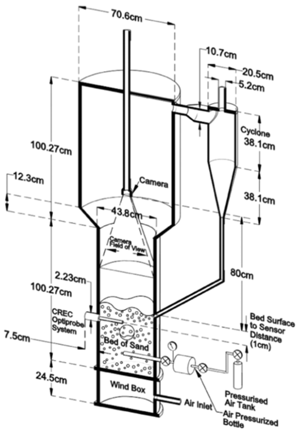
Figure 1. Schematic diagram of the cold gasifier sand fluidized bed unit including its dimensions [20].
Processes 14 03002 g001
Figure 2. Particle size distribution of the SiO2 sand particles.
Processes 14 03002 g002
Figure 3. Schematic diagram of the fluidized bed [8].
Processes 14 03002 g003
Figure 4. (a). Radial distribution of the time-average particle volume fraction for the coarse, medium and fine meshes, for a mass air flow rate of 0.0405 kg/s. (b). BRVs and BACs for the coarse, medium and fine meshes, for a mass air flow rate of 0.0405 kg/s.
Processes 14 03002 g004
Figure 5. 3D view of the CPFD data collection points from the simulated detection system for assessing fluid dynamics in the sand bubble fluidized bed at several radial positions.
Processes 14 03002 g005
Figure 6. Characteristic signal obtained from the upper and lower virtual probes implemented in the CPFD simulations for computational bubble identification and hydrodynamics parameter determination.
Processes 14 03002 g006
Figure 7. Comparation of emulsion and bubbles phase volumetric fraction data obtained in experiments and that acquired in CPFD simulations at various radial positions of the sand fluidized bed. Note: Reported error bars represent standard deviations for 3 repeat measurements at the considered radial position. For the sand measurements, RMSE = 0.0497, and for the bubbles, RMSE = 0.528 when comparing experimental and simulation results.
Processes 14 03002 g007
Figure 8. Comparation of radial distributions of average biomass pellet volumetric fraction obtained experimentally and in CPFD simulations at different radial positions. Note: Reported error bars represent standard deviations for 3 repeat measurements at the considered radial position. RMSE = 0.00681 when comparing experimental and simulation results.
Processes 14 03002 g008
Figure 9. BRVs as function of BACs obtained from experimental data and CPFD barracuda simulations.
Processes 14 03002 g009
Figure 10. BRV-BAC comparison for single bubble injection and CPFD simulated bubbles in a sand fluidized bed at minimum fluidization.
Processes 14 03002 g010
Figure 11. Comparison of the BRVs obtained from experiments using (1) CREC-GS-Optiprobes (black squares), (2) CPFD data (green squares), (3) CPFD data adjusted using Equation (19) (blue triangles and (4) model data from Equation (18) (full line) at the following superficial gas velocities: (a) 0.250 m/s, (b) 0.281 m/s and (c) 0.344 m/s.
Processes 14 03002 g011
Table 1. CPFD Barracuda parameters.
VariableValue
Simulation duration300 s
Close-packed volume fraction0.66
Normal-to-wall momentum retention0.80
Tangent-to-wall momentum retention0.80
Maximum momentum redirection from collision (%)40
Diffuse bounce3.00
Base materialsAir (default parameters), SiO2 (ρ = 2650 kg/m3) and Wood-Pellets (ρ = 550 kg/m3)
Fluid initial conditionsP = 101 KPa
v = 0 m/s
Convergence criteria Volume–10 iterations (1 × 10⁻⁷ residual)
Pressure–2000 iterations (1 × 10⁻⁶ residual)
Velocity–50 iterations (1 × 10⁻⁷ residual)
Drag model–Sand particlesWen–Yu–Ergun model
Drag model–Biomass particlesnon-spherical Haider–Levenspiel model
Sand particle mass (kg)114.30
Biomass particle mass (kg)0.93
Sphericity–Sand particles0.90
Sphericity–Biomass particles0.75
CFL range0.80–1.50
Time step (s)0.055–0.041
Total number of particles4.53 × 108
Total number of clouds2.74 × 106
Particle size distributionSame as shown in Figure 1
Table 2. CPFD Barracuda boundary conditions.
Volumetric Flow
(SCFM)
Mass Flow Rate
(kg/s)
Gas Velocity (m/s)Pressure Fluid
Bed Inlet
(KPa)
Pressure Fluid
Bed Outlet
(KPa)
800.0450.250111.9104.5
900.0510.281112.8105.5
1100.0620.344114.8107.4
Table 3. Grid independence test analysis results for a mass air flow rate of 0.0405 kg/s.
MeshNumber of CellsΔP
(KPa)
Fluid Mass Flux
(kg/sm2)
Particle Mass Flux STD
(kg/sm2)
Coss-Sectional Average PVF
Coarse10,6567.2200.26943.530.625
Medium87,0406.7130.27019.210.615
Fine664,0206.8210.26911.080.609
Table 4. Comparison of RMSE at various superficial gas velocities and α values.
U (m/s)αRMSE
Exp vs. Equation (18)
RMSE
CPFD vs. Equation (18)
RMSE
CPFDcorrected vs. Equation (18)
0.2506.490.2530.4930.068
0.2814.990.2280.5640.062
0.3442.960.2760.4220.143
Note: The parameter γ from Equation (18) is set at 0.5.
Disclaimer/Publisher’s Note: The statements, opinions and data contained in all publications are solely those of the individual author(s) and contributor(s) and not of MDPI and/or the editor(s). MDPI and/or the editor(s) disclaim responsibility for any injury to people or property resulting from any ideas, methods, instructions or products referred to in the content.