Article

Annulus Back-Pressure Transfer Law During Managed-Pressure Cementing Process in Ultra-Deep Wells


1
R&D Center for Ultra Deep Complex Reservior Exploration and Development, China National Petroleum Corporation, Korla 841000, China
2
Engineering Research Center for Ultra-Deep Complex Reservoir Exploration and Development, Xinjiang Uygur Autonomous Region, Korla 841000, China
3
Xinjiang Key Laboratory of Ultra-Deep Oil and Gas, Korla 841000, China
4
PetroChina Tarim Oilfield Company, Korla 841000, China
5
China National Petroleum Corporation Engineering Technology R&D Company Limited, Beijing 102200, China
*
Author to whom correspondence should be addressed.
Processes 2026, 14(16), 2611; https://doi.org/10.3390/pr14162611
Submission received: 11 May 2026 / Revised: 14 July 2026 / Accepted: 27 July 2026 / Published: 17 August 2026

Abstract

The formation pressure system of ultra-deep wells is complex, and managed pressure cementing (MPC) is a commonly used technical means of safety control and cementing quality improvement. During the MPC process, pump switching operations can induce substantial annular back-pressure. The attenuation of annular back-pressure within the wellbore serves as a pivotal foundation for the precise determination of back-pressure compensation values in ultra-deep wells. Building upon the one-dimensional transient flow model of the wellbore, we developed a transient transmission model for annular back-pressure and solved it using the finite difference method. The computational results were validated against experimental data, thereby elucidating the attenuation pattern of annular pressure waves in ultra-deep wells. The findings reveal that the primary controlling factors for the attenuation of pressure waves encompass well depth, the elastic modulus of the wellbore rock, and the rheological model of the drilling fluid. As well depth increases, the pressure wave exhibits a linear decrease, with discontinuities occurring at the casing and open-hole sections. The rate of pressure wave attenuation accelerates within the open-hole interval. The lower the elastic modulus of the open-hole segment, the more rapid the attenuation rate of the pressure wave becomes. The attenuation laws of annular fluids with different rheological models are ranked as follows: Power-law model > Herschel–Bulkley model > Bingham model. Under the computed well conditions, the pressure of the power-law fluid decreases to 85% of its initial back-pressure value. This research provides theoretical underpinnings for the design and execution of on-site MPC operations.

1. Introduction

MPC technology serves as a pivotal approach for ensuring safe and efficient cementing operations within narrow pressure windows. Throughout the MPC process, the phase involving pump shutdown and packer setting entails pump start/stop maneuvers, which induce transient fluctuations in annular back-pressure. Owing to the compressibility of the fluid within the annulus, the annular back-pressure undergoes attenuation, consequently diminishing the pressure reaching the bottom of the well [1]. Should pressure compensation not be executed promptly or if the pressure fails to attain the requisite level, it could potentially compromise the safety of the wellbore.
Numerous scholars have conducted in-depth research on the attenuation and change law of pressure waves and have put forward a variety of ideas and methods for solving models. Zhou et al. [2] established a propagation model of pressure waves in viscous fluids by studying the propagation characteristics of pressure in viscous fluids and derived the propagation expressions of pressure waves. Pierre et al. [3] studied the propagation of pressure waves in pipelines by the finite volume method. Li et al. [4] proposed a numerical method for predicting pressure wave velocity. Guo et al. [5] used FLUENT software to establish a two-dimensional model of the pipeline system and studied the propagation law of pressure waves in leaking pipes. Yang et al. [6] found that the existence of pipeline leakage holes will lead to distortion of pressure wave propagation. Chen [7] analyzed the propagation of pressure waves in variable-section thick-walled viscous incompressible fluid pipelines based on the wave reflection factors of the pipe end face during arterial pulse wave propagation. Yu [8] considered the influence of velocity distribution and heat transfer in the fluid, the dissipation mechanism of the pressure wave propagation system is derived, and the dissipation of the pressure wave on the gas-phase laminar flow is predicted. Yuan et al. [9] proposed applying the eigenline method to solve the basic partial differential equations of unsteady flow in pipelines and analyzed the transient fluctuations of complex pipeline systems. Wu et al. [10] used the characteristic line method to solve the continuous equations and momentum equations of the transient annulus system of aero engines, and obtained the changes in pressure, mass flow, and temperature of the fluid in the annulus system with time by simulating the system. Shi et al. [11] combined experiment with the characteristic line method (MOC) to predict the maximum water hammer pressure generated at the time of valve closing in the pipe network and analyzed the influence of the valve closing time and the valve closing law on the maximum water hammer pressure. Fu et al. [12] used experimental testing and numerical simulation methods to study the pressure transient phenomenon of hydraulic systems and developed a pressure transient prediction and control engineering application software in the MATLAB environment to numerically simulate the unsteadily flowing micro-compressed fluid in the tube. Diao et al. [13] introduced a one-dimensional unsteady flow equation based on an improved system leak detection model, used the characteristic line method to solve the model, and analyzed the transient changes in pressure waves to detect pipeline leakage location. Sondermann et al. [14] proposed a one-dimensional transient numerical model to simulate the two-phase gas–liquid flow and analyzed the applicability of the model. Based on the physical properties of supercritical carbon dioxide, Ding et al. [15] constructed a thermal–fluid–solid coupling transient fluctuation pressure model at the bottom of the wellbore, which considers the heat transfer between carbon dioxide and the drill string and the wellbore wall, and studied the transient changes in bottom-hole pressure. Sha et al. [16] developed a computer-controlled test device for the transient characteristics of self-circulating steady flow pipelines to test and measure water hammer pressure waves and revealed the propagation mode and characteristics of water hammer pressure waves. Zhang et al. [17] provided the pressure wave fluctuation equation and the solution conditions for the dynamic string in each flow channel in the well, and used the mixed implicit eigenline method to solve the equation to obtain the numerical solution of the transient pressure. Yan et al. [18] solved and analyzed the propagation law of the back-pressure pressure wave in the gas–liquid two-phase medium of the annulus by establishing a back-pressure pressure wave propagation model, and found that the velocity of the pressure wave decreases sharply when a very small amount of gas is mixed into the liquid phase, and the decrease in the pressure wave velocity slows down with the increase in gas in the liquid phase. Wang et al. [19] established a pressure decay model in the two-phase flow of managed pressure drilling based on the dual-fluid model and used small disturbance theory and the semi-implicit difference method to solve the model, and analyzed the influence of temperature, pressure, and void ratio on the pressure attenuation coefficient. Yu et al. [20] established a calculation model of the propagation velocity of back-pressure in the annulus, and analyzed the influence of gas content, rock chip content, and drilling fluid density on the back-pressure propagation velocity. Based on fluid mechanics, Ding [21] established a theoretical model of the attenuation of the wellhead pulse pressure in the annulus, and analyzed the effects of the pulse pressure amplitude, initial shear force of cement slurry, and annulus fluid compression coefficient on the attenuation law of pulse pressure. For the propagation characteristics of the back-pressure pressure wave in the medium and the solution of the model equation, many theoretical and experimental studies have been carried out, and much useful information has been provided. However, the existing research results are mainly aimed at multiphase flow systems, and the pressure wave transmission conditions of MPC are mainly affected by the rheological mode and fluid type of the annulus fluid.
Based on the one-dimensional transient flow model of the wellbore, the transient pressure wave transmission model of the annulus back-pressure of MPC is established by intercepting the annulus microelements for force analysis, the finite difference idea is introduced to solve it, and the transmission law of transient annulus back-pressure of MPC is explored.

2. Mathematical Model

2.1. Conditional Assumptions

When establishing the transient pressure wave transmission model of MPC annulus back-pressure, the following assumptions are made:
Assumption 1.
The propagation process of pressure waves in the annulus is an irreversible adiabatic process.
Assumption 2.
The one-dimensional liquid phase flow of the fluid along the wellbore direction is considered.
Assumption 3.
In the cross-sectionally averaged one-dimensional formulation, the momentum equation is written in terms of the external forces: pressure forces, gravity, and wall shear stress. The internal shear stress between adjacent fluid layers is not explicitly listed as an external force term because it cancels in the overall force balance of the element and, more importantly, is implicitly accounted for through the rheological constitutive equations (Equations (6), (12) and (17)) when relating the mean velocity to the wall shear stress. For annular flow, the shear stress distribution follows τ(r) = τ_w · (r − R_i)/(R_o − R_i), and the internal shear gradients are embedded in the rheological parameters (K, n, τ0) via the friction factor correlation. Therefore, this treatment introduces no additional error beyond the inherent accuracy of the cross-sectional averaging procedure.
Assumption 4.
Interfacial mixing between different liquid-phase media (drilling fluid, preflush, and cement slurry) is neglected, and the interfaces are treated as sharp boundaries; cross-sectional exchange of mass and momentum between adjacent fluid layers is also neglected.
Assumption 5.
The present single-phase model is applicable to conditions where the gas void fraction in the annulus is negligible (i.e., αg < 0.5%). In practice, managed pressure cementing (MPC) operations are designed to maintain a positive overbalance pressure to prevent gas influx during the cementing phase. For cases where gas influx is anticipated or gas-cut mud is present, the model can be extended to two-phase flow by incorporating the gas-phase continuity and momentum equations, which will be addressed in our future work.
Justification of the assumptions for ultra-deep well applications. The validity of the above assumptions under ultra-deep-well conditions deserves explicit discussion, as such environments typically feature elevated down-hole temperatures (exceeding 150 °C), high pressures (over 150 MPa), and extended wellbore lengths (7000 m or deeper), all of which may potentially challenge the simplifications adopted in the model.
For Assumption 1 (adiabatic process), the characteristic time of pressure wave propagation through a 7000 m annulus is on the order of several seconds, whereas the characteristic time for thermal conduction between the fluid and the surrounding formation is typically several minutes to hours, given the low thermal diffusivity of drilling fluids and rock. Thus, the adiabatic treatment introduces negligible error. For Assumptions 2 and 5 (one-dimensional single-phase liquid flow), the wellbore deviation in ultra-deep exploratory wells (such as Well XX-1 in Section 3.4) is generally kept below 15° to facilitate casing running and cementing operations, which justifies neglecting radial velocity components. Additionally, the positive overbalance pressure maintained throughout MPC operations effectively suppresses gas influx, ensuring that the gas void fraction remains below 0.5%, as stated in Assumption 5. For Assumption 3 (cross-sectional averaging), ultra-deep well annuli are characterized by large length-to-hydraulic-diameter ratios (exceeding 2000:1 in the case presented), allowing the flow to be treated as fully developed over the majority of the annulus. The internal shear stress gradients, though physically present, are not neglected but rather are embedded in the rheological constitutive equations (Equations (6), (12) and (17)) and the corresponding wall shear stress formulations, a standard treatment in one-dimensional non-Newtonian flow modeling that has been extensively validated for annular geometries in drilling engineering. For Assumption 4 (negligible intermixing), while some mixing at fluid interfaces inevitably occurs, the volumes of mixed zones are small relative to the total annular volume, and the compressibility differences among drilling fluid, Pref lush, and cement slurry are minor compared to those between liquid and gas phases. Consequently, treating the interfaces as sharp boundaries does not significantly affect the pressure wave attenuation predictions. The experimental validation in Section 2.4, with errors within ±7.4%, further corroborates the overall reasonableness of these simplifications for engineering practice.
Quantitative assessment of the sharp-interface assumption. To evaluate the effect of neglecting interfacial mixing between different fluids (drilling fluid, preflush, and cement slurry), a sensitivity analysis was performed. The results indicate that even with mixing zone thicknesses of up to 50 m at the fluid interfaces, the deviation in predicted bottomhole pressure remains well below 1% compared with the ideal sharp-interface model. This confirms that the sharp-interface assumption is reasonable for the pressure wave attenuation predictions in ultra-deep wells.

2.2. Model Creation

2.2.1. Control Equations

As shown in Figure 1, the dz segment of the annulus is taken as a microelement, and the flow cross-section is A, the density ρ, and the velocity v changes with time and position: ρ = ρ(z,t), v = v(z,t). The fluid flows in from section 1 and flows out from section 2, the distance between the two sections is dz, the initial flow rate is v0, and the initial density of the fluid is ρ.
The arrows denote the external forces (pressure, gravity, and wall shear). The internal shear stress between adjacent fluid layers is an internal force and is not shown separately; its effect is implicitly incorporated through the rheological constitutive equations (Equations (6), (12) and (17)) in the cross-sectionally averaged formulation.
According to the conservation theorem of mass, the continuity equation of the microelement segment of the fluid is written as
z ( ρ v ) + ρ t = 0
In the formula: ρ is the fluid density, kg/m3; v is the fluid velocity, m/s; t is time, s; z is the well depth (along the wellbore direction), m.
According to the conservation of momentum theorem, the momentum equation for liquid phase flow can be written as
t ( ρ v ) + z ( ρ v 2 ) = ρ g p z 4 τ w d hy
where τw is the viscous shear stress between the fluid and the wellbore wall, Pa; dhy is the hydraulic diameter of the annulus, m.
d h y = 2 R δ
The meanings of the symbols in the formula are the same as before, and d_hy is defined as the hydraulic diameter of the annulus in meters.

2.2.2. Modulus of Elasticity

From the definition of elastic modulus, it can be seen that the pressure and density of a fluid have the following relationship [22]:
K = d P d ρ / ρ
In the formula: K_f is the bulk modulus of the fluid, Pa; p is the pressure, Pa.
Available
p = p 0 + K ln ρ ρ 0
In the momentum equation, the viscous shear stress between the fluid and the wellbore wall is related to the rheological mode of the fluid [23].
  • Power-law mode
Flow Equation:
Q = n π 2 n + 1 R o + R i R δ ( Δ P K L ) 1 n ( R δ 2 ) n + 1 n
In the formula: K is the consistency coefficient, in Pa·sn; n is the flow behavior index, dimensionless; γ is the shear rate, in s−1.
Annulus cross-sectional area:
A = π ( R o 2 R i 2 )
In this formula: A is the cross-sectional area of the annular flow, in m2; R_o is the outer radius of the annulus (wellbore radius), in meters; R_i is the inner radius of the annulus (outer radius of the tubing), in meters.
Average Flow Velocity of Annulus Fluid:
v 0 = n 2 n + 1 Δ P K L 1 n ( R δ 2 ) n + 1 n
In the formula: v0 is the average flow speed of the hollow fluid, in meters per second (m/s).
Viscous shear stress:
τ w = R δ 2 K ( n 2 n + 1 ) n ( R δ 2 ) n + 1 v 0 n
In the formula: τw: Wall viscous shear stress; R_δ: Characteristic radius of the annular gap; K: Consistency coefficient of the power-law fluid; n: Flow behavior index of the fluid; v_0: Average fluid velocity in the annulus; Conservation of momentum equation:
( ρ v ) t + ( ρ v 2 ) z + p z + ρ g + 1 K ( n 2 n + 1 ) n ( R δ 2 ) n + 1 v 0 n = 0
The flow rate coefficient b:
b = 1 K ( n 2 n + 1 ) n ( R δ 2 ) n + 1
2.
Bingham model
Flow Equation:
Q = Δ p π ( R o + R i ) 12 μ p L R δ 3 π ( R o + R i ) R δ 2 4 μ p τ 0
In the formula: τ0 is the yield stress, Pa; μ_p is the plastic viscosity, Pa·s.
Average Flow Velocity of Annulus Fluid:
v 0 = Δ p R δ 12 μ p L R δ τ 0 4 μ p
Viscous shear stress:
τ w = 6 μ p v 0 + 1.5 R δ τ 0
Conservation of momentum equation:
( ρ v ) t + ( ρ v 2 ) z + p z + ρ g + 3 τ 0 + 12 μ p R δ v 0 = 0
Flow rate coefficient b:
b = 12 μ p R δ
3.
Herschel–Bulkley model
Flow Equation:
Q = n π R δ 2 2 ( 2 n + 1 ) K 1 n ( R o + R i ) ( Δ p R δ 2 L Δ p R δ 2 L ) 1 n
The meanings of the symbols in this formula are the same as in Formulas (6) and (12).
Average Flow Velocity of Annulus Fluid:
v 0 = n R δ 2 ( 2 n + 1 ) K 1 n ( Δ p R δ 2 L 2 n + 1 n + 1 τ 0 ) 1 n
Viscous shear stress:
τ w = K 2 ( 2 n + 1 ) n R δ n v 0 n + 2 n + 1 n + 1 τ 0
Conservation of momentum equation:
( ρ v ) t + ( ρ v 2 ) z + p z + ρ g + 2 n + 1 R δ ( n + 1 ) τ 0 + 2 K 2 ( 2 n + 1 ) n R δ n R δ v 0 n = 0
Flow rate coefficient b:
b = 2 K 2 ( 2 n + 1 ) n R δ n R δ
Among them, ρ is the fluid density, v0 is the average flow velocity of the annulus fluid, K is the consistency coefficient, n is the fluidity index, τ0 is the dynamic shear force, Ro is the outer diameter of the annulus, and Ri is the inner diameter of the annulus.

2.3. Model Solving

According to the finite difference idea [24,25,26,27,28,29], the momentum equation and the continuity equation are discretized in time and space, respectively, and the pressure decay law is found by solving the pressure at different depths.

2.3.1. Numerical Parameters

All simulations in this study were performed with a spatial step of Δz = 50 m, refined to Δz = 25 m near the bottom-hole section (5000–7000 m). The corresponding time step was set to Δt = 0.005 s for the coarse grid and Δt = 0.0025 s for the refined region. The Courant–Friedrichs–Lewy (CFL) number for the explicit finite difference scheme is defined as CFL = v·Δt/Δz. With a maximum fluid velocity v ≤ 2.0 m/s in the annulus, the maximum CFL number is 2.0 × 10⁻⁴, which is far below the stability limit of CFL ≤ 1.0 for the explicit scheme. Thus, the numerical scheme is unconditionally stable for all cases considered in this study.

2.3.2. Equation Discretization

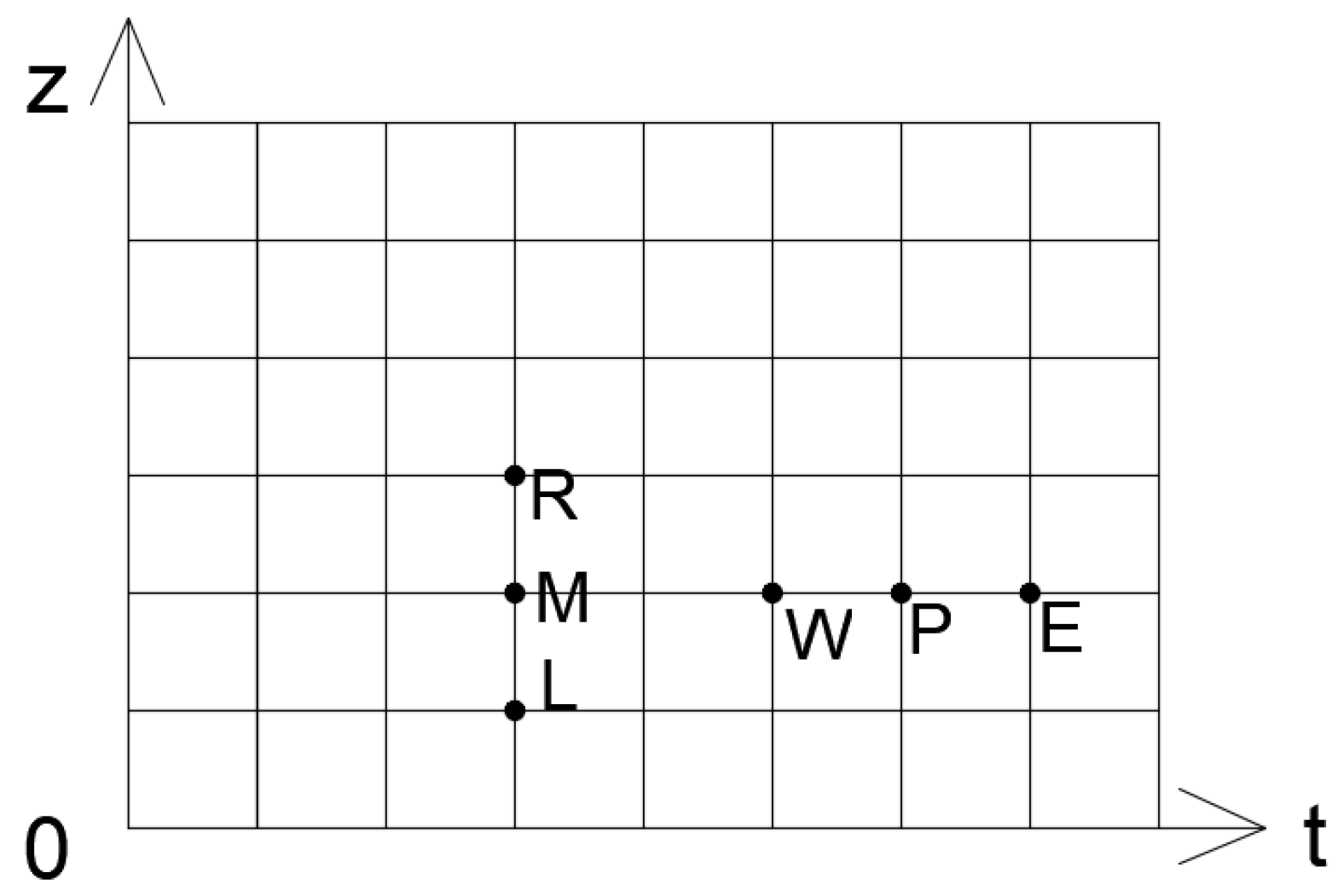
In the discrete grid diagram of Figure 2, z and t are the spatial and temporal coordinate axes, R, L, and M are points at different positions at the same time, and W, P, and E are points at different times in the same position.
Momentum Equation Discretization:
t ρ v M = v M ρ v R ρ v L 2 Δ z p R p L 2 Δ z b v M n ρ R ρ L g
In the formula: Subscript M: current central grid node; Subscript R: right grid node; Subscript L: left grid node; b: viscous resistance coefficient;
ρ M t v M t + Δ t ρ M t v M t Δ t = v M t ρ v R t ρ v L t 2 Δ z p R t p L t 2 Δ z b ( v M t ) n ρ R t ρ L t g
The velocity of any point M at the moment t + Δt:
v M t + Δ t = v M t + v M t Δ t ρ v L t ρ v R t + Δ t p L t p R t + g Δ t ρ L t ρ R t 2 Δ z Δ t b ( v M t ) n 2 Δ z ρ M t
In the formula:
Suppose there are n points in a one-dimensional space, if i is in the range of (2, n − 1), then
v i t + Δ t = v i t + v i t Δ t ρ v i 1 t ρ v i + 1 t + Δ t p i 1 t p i + 1 t + g Δ t ρ i 1 t ρ i + 1 t 2 Δ z Δ t b ( v i t ) n 2 Δ z ρ i t
Discretization of the continuity equation:
ρ t p + ρ v E ρ v W 2 Δ z = 0
ρ P t + Δ t ρ P t Δ t + ρ E t v E t + Δ t ρ W t v W t + Δ t 2 Δ z = 0
Density of any point P at the moment t + Δt:
ρ P t + Δ t = ρ E t v E t + Δ t ρ W t v W t + Δ t Δ t 2 Δ z + ρ P t
For 2 ≤ i ≤ n − 1, then
ρ i t + Δ t = ρ i 1 t v i 1 t + Δ t ρ i + 1 t v i + 1 t + Δ t Δ t 2 Δ z + ρ i t

2.3.3. Initial and Boundary Conditions

(1)
There is only drilling fluid in the annulus
p ( z , t ) z = 0 = p B P 0
(2)
There are drilling fluids and preflushes in the annulus
p ( z , t ) z = 0 = p B P 0 p ( z , t ) z = h 1 = p B P 1
Among them, H1 is the preflush deepening; P back-pressure value 1 is the back-pressure value at the bottom of the drilling fluid.
(3)
There are drilling fluids, prefluids, and cement slurries in the annulus
p ( z , t ) z = 0 = p B P 0 p ( z , t ) z = h 1 = p B P 1 p ( z , t ) z = h 2 = p B P 2
Among them, h1 is the preflush deepening; pBP1 is the back-pressure value at the bottom end of the drilling fluid; h2 is the depth of the cement slurry; pBP2 is the back-pressure value at the bottom of the pre-liquid.

2.3.4. Pressure Calculation

The pressure p of any point in each fluid segment in the annulus has the following relationship with the density ρ of the point:
p i = p i 0 + K ln ρ i ρ i 0
In the formula: ρ_{i0} is the density of the ith fluid at the reference pressure p_{i0}, in kg/m3; p is the pressure at any point, in Pa; when i = 1, it means the annulus contains only drilling fluid, i = 2 means it contains drilling fluid and spacer fluid, and i = 3 means it contains drilling fluid, spacer fluid, and cement slurry.
Where ρi0 is the density of the fluid at a certain pressure pi0, i = 1, 2, 3; When i = 1, only drilling fluid exists in the annulus. When i = 2, drilling fluid and preflush fluid exist in the annulus; When i = 3, the annulus fluid is drilling fluid, preflush fluid, and cement slurry.
Using the joint vertical Equations (25), (29) and (33) and substituting the initial and boundary conditions to solve the solution the back-pressure value at each position in the annulus can be obtained.

2.4. Model Validation

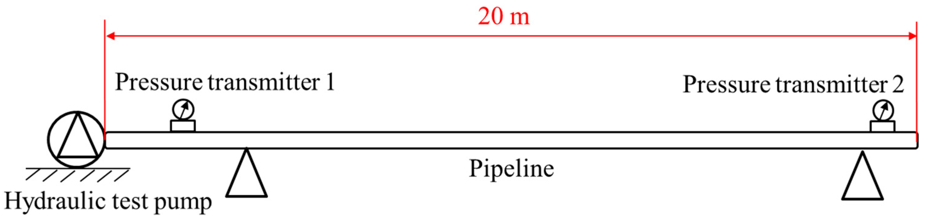
In order to verify the accuracy of the pressure wave transient transmission model of MPC annulus back-pressure, a pressure wave attenuation simulation laboratory experiment was carried out by the Wave pressure testing device (CNPC Engineering Technology R&D Company Limited, Beijing, China), as shown in Figure 3. A quantity of 2.0 g/cm3 of drilling fluid was used as the experimental fluid and the drilling fluid was pumped into the cavity by a high-pressure piston pump; the pumping flow rate was 0.025 m3/s. The inner diameter of the cavity was 12 cm, the length was 20 m; the initial pressure was given by the nitrogen cylinder pressurization, and the pressure sensors installed monitored the pressure value at both ends of the cavity.
The pressure wave attenuation experiments under pressure of 3 MPa, 2.5 MPa, 2 MPa, 1.5 MPa, 1 MPa were carried out by this device. Comparing the experimental results with the calculation results of the model, as shown in Table 1, it can be seen that the pressure value measured in the experiment is not much different from the calculated value of the model and the error is within ±7.4%, so the transient pressure wave transfer model can be used to calculate the pressure attenuation.

2.5. Scaling Analysis from Laboratory to Field Scale

A significant scale gap exists between the 20 m laboratory test cavity and the 7000 m ultra-deep field wellbore. To address this gap, a scaling analysis is provided based on the governing equations.
(1)
Length scale. The pressure wave attenuation process is governed by the same one-dimensional transient flow equations at both laboratory and field scales. The per-unit-length pressure attenuation rate in the laboratory experiments is of the same order of magnitude as that in the field casing section, confirming the consistency of the underlying physical mechanism.
(2)
Diameter scale. The annular hydraulic diameters in the laboratory cavity and in the field wellbore are within the same order of magnitude (less than 30% difference), ensuring that the wall shear stress contributions remain comparable between the two scales.
(3)
Temperature and pressure effects. The model implicitly accounts for temperature and pressure effects through the fluid bulk modulus Kf and the elastic modulus E of the wellbore rock and casing, both of which are temperature- and pressure-dependent in the field application. The governing equations for transient pressure wave propagation are form-invariant, with the speed of sound as the characteristic velocity, which justifies the extrapolation of laboratory-validated results to field conditions.
Based on the above analysis, the laboratory validation provides a reasonable and conservative basis for evaluating the model’s performance at the field scale.

3. Influencing Factors and Example Analysis of Back-Pressure Attenuation

In order to further study the attenuation characteristics of back-pressure pressure waves in annulus liquid-phase fluids, a numerical calculation of the attenuation characteristics of back-pressure pressure waves in down-hole was carried out using the established transient pressure wave transmission mathematical model.
The relevant parameters used in the calculation are as follows: the well depth is 7000 m, the outer diameter of the casing is 139.7 mm, the outer diameter of the upper casing is 244.5 mm, the lower depth of the upper casing is 5000 m, and the diameter of the wellbore is 215.9 mm; the density of drilling fluid is 2.0 g/cm3; the elastic modulus of the formation is 40 GPa, and the elastic modulus of the casing is 206 GPa. The initial back-pressure value is 5 MPa, and the rheological mode of the drilling fluid adopts the Herschel–Bulkley rheological model.

3.1. Variation Law of Annulus Back-Pressure with Well Depth

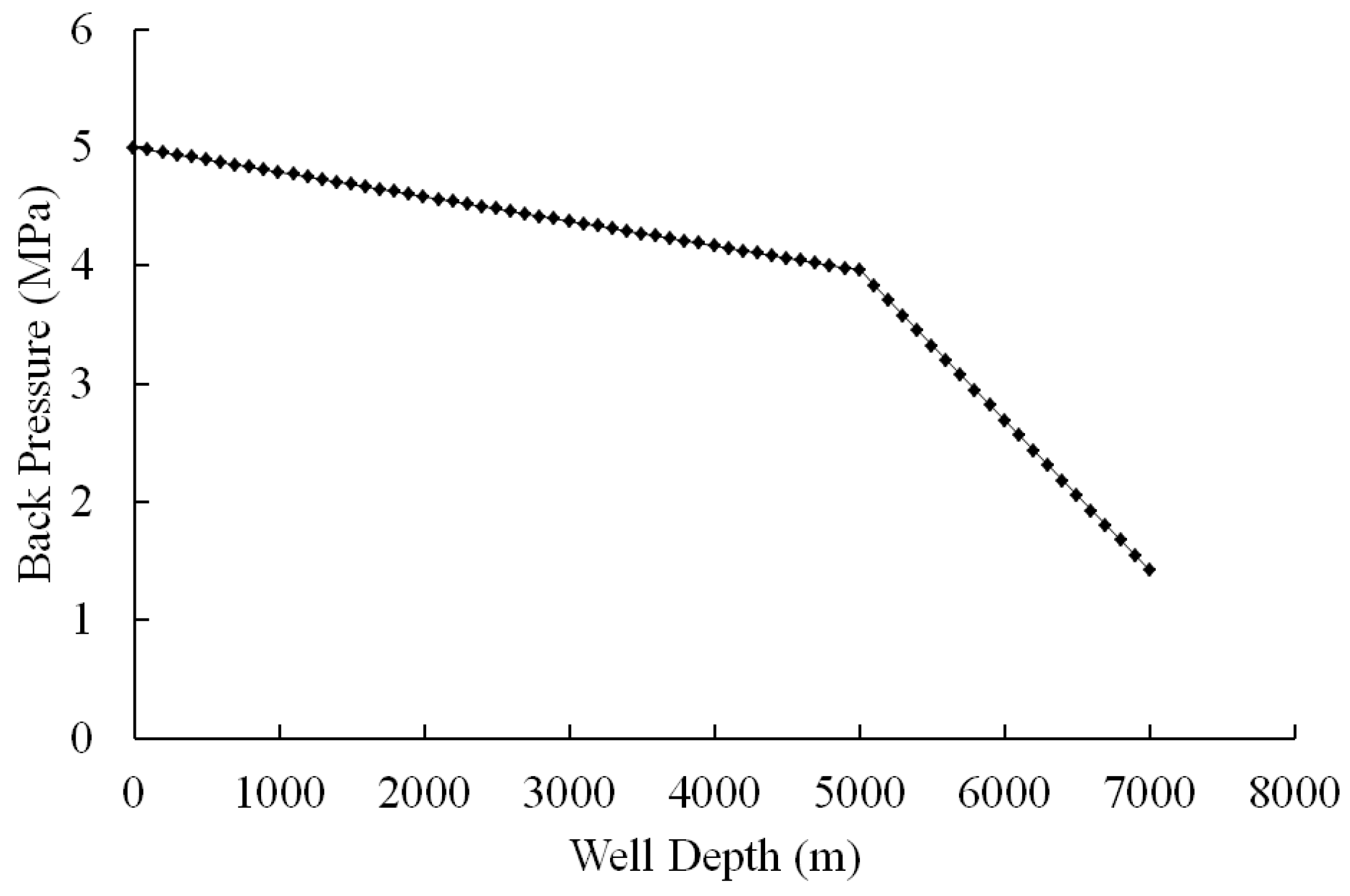
Under the condition of an annulus back-pressure of 5 MPa, the change in pressure wave with well depth is shown in Figure 4.
It can be seen from the figure that with increase in well depth, the back-pressure value gradually decreases, and there is a turning point at 5000 m The pressure loss above the turning point is 0.0208 MPa/100 m, and the pressure loss below the turning point is 0.127 MPa/100 m. Above the turning point is the upper casing section. Due to the large elastic modulus of the upper casing, the energy loss is small during the pressure wave transmission. Below the turning point is the open-hole section, which has a relatively small elastic modulus, shows relatively easy deformation, and has a large ability to absorb pressure waves.
It can be seen that the elastic modulus is an important factor affecting the loss of pressure waves. The influence of the formation elastic modulus on pressure wave attenuation will be described in the next section.

3.2. Elastic Modulus of Rock in the Wellbore

In order to explore the influence of the elastic modulus of wellbore rock on the attenuation of pressure waves, the pressure waves of different elastic modulus of wellbore rocks and the bottom well pressure values of different upper casing depths were calculated.
(1)
The elastic modulus of the rock in the well wall
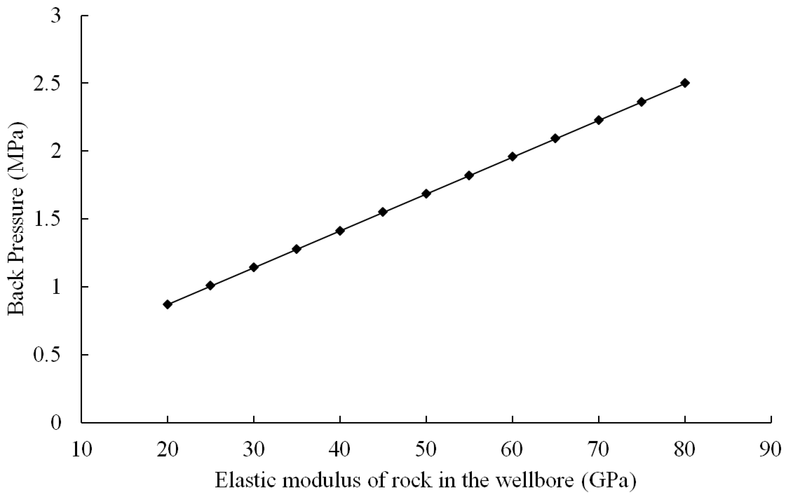
According to the performance parameters of different rocks, the elastic modulus of rock in the well wall is set as 20 GPa, 25 GPa, 30 GPa, 35 GPa, 40 GPa, 45 GPa, 50 GPa, 55 GPa, 60 GPa, 65 GPa, 70 GPa, 75 GPa, and 80 GPa. The influence of the elastic modulus of rock on the bottom pressure wave of the wellbore wall is calculated as shown in Figure 5.
It can be seen from the figure that with increase in the elastic modulus of the rock in the wellbore, the pressure transmitted to the bottom of the wellbore increases approximately linearly, that is, the attenuation of annulus pressure decreases. For MPC, the elastic modulus of the ground layer is small, and the compensation value of the annulus back-pressure should be increased to compensate for the requirement that the bottom-hole pressure cannot reach the safe value due to the attenuation of the pressure wave.
(2)
Upper casing depth
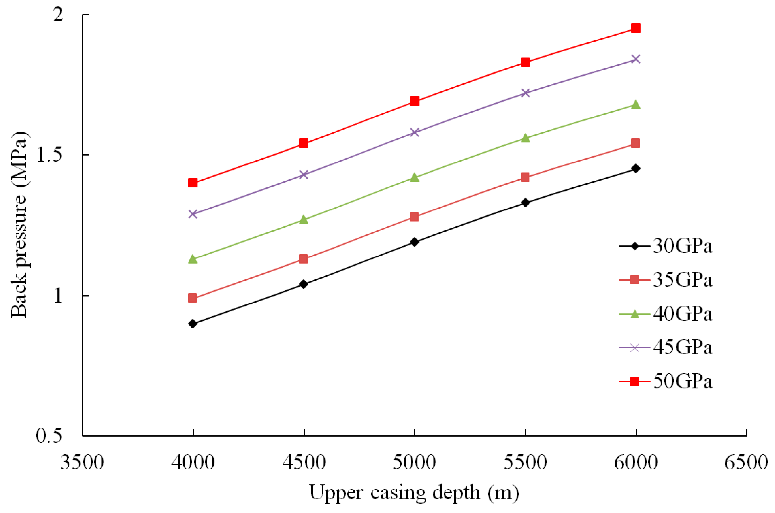
To investigate the combined effect of casing shoe depth and the formation elastic modulus on pressure wave attenuation, five casing shoe depths (4000 m, 4500 m, 5000 m, 5500 m, and 6000 m) and five elastic modulus values (30 GPa, 35 GPa, 40 GPa, 45 GPa, and 50 GPa) were selected for parametric analysis. The selected elastic modulus range covers the typical values of sandstone formations in the target block, and the casing shoe depth range corresponds to the commonly used casing design schemes for ultra-deep wells. The five discrete modulus values were chosen at 5 GPa intervals across the full typical range to provide adequate resolution for revealing the attenuation trend (as established in Figure 5). The computed bottom-hole pressures under different combinations of these two parameters are presented in Figure 6.
(3)
Practical estimation of elastic modulus from logging data
A practical method for estimating the elastic modulus from logging data is as follows: when both the shear and compressional wave transit times are available, the dynamic elastic modulus E d is calculated by the formula
E d = ρ b × 1 t s 2 × 3 t s 2 4 t c 2 t s 2 t c 2
where ρ b is the bulk density (g/cm3), and Δ t s and Δ t c are the shear and compressional transit times (μs/m), respectively; if only compressional data are available, then for sandstone with porosity less than 15% E 0.035 v p 2 is used, and for mudstone E 0.022 v p 2 is used (with v p in km/s and E in GPa), and these empirical estimates typically have an uncertainty of ±15% to ±25%. A sensitivity analysis shows that with a baseline of 40 GPa, a ±20% variation in the elastic modulus results in bottom-hole pressure changes of about −6.8% and +5.9%, respectively, with a sensitivity of approximately 0.32 MPa/GPa; accordingly, a ±15% modulus estimation error translates into about ±4.5% error in bottom-hole pressure prediction, which falls within acceptable engineering tolerances.

3.3. Influence of Rheological Patterns

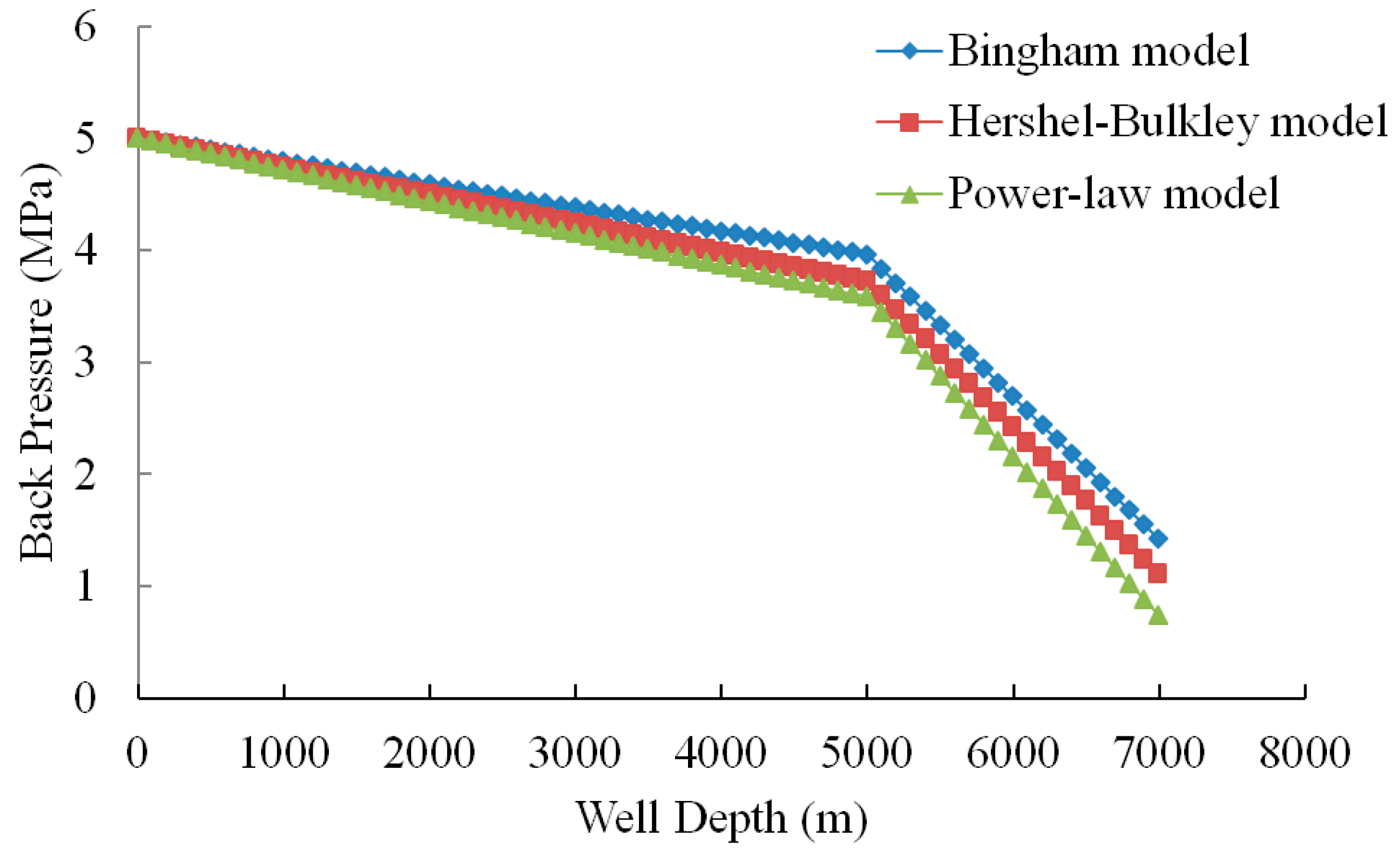
Rheological mode is one of the main factors affecting the attenuation of the back-pressure pressure wave, and Figure 7 shows the attenuation of the same fluid when the same back-pressure value reaches the bottom of the wellbore under different rheological modes. The back-pressure attenuation curves of different rheological modes are shown in Figure 8. When the fluid is in power-law mode, the pressure wave attenuates the most, and the pressure wave decreases from the original 5 MPa to 0.74 MPa, and the pressure is reduced by 85%.
The attenuation ranking (Power-law > Herschel-Bulkley > Bingham) is governed by two competing mechanisms: shear-thinning promotes momentum dissipation, while yield stress impedes it. Under the specific fluid parameters employed in this study, shear-thinning dominates; hence, the power-law fluid—whose apparent viscosity decreases with declining shear rate during pump shutdown—exhibits the strongest attenuation, whereas the Bingham fluid, possessing a yield stress that retards dissipation at low shear rates, exhibits the weakest. The Herschel–Bulkley fluid, combining both characteristics, yields an intermediate behavior.

3.4. Case Studies

Taking the pressure transfer law during MPC operation of 139.7 mm diameter oil well casing in Well XX-1 as the research object, a field case analysis was carried out. Well XX-1 is a risk exploration well in Xinjiang Oilfield, which has been drilled to a depth of 7050.00 m. The position of the upper casing shoe is 4950 m. The leakage layer is at 5200 m of the well, and the pore pressure equivalent density and leakage pressure equivalent density of the formation are 1.95 g/cm3 and 2.08 g/cm3, respectively. There is a high-pressure layer at 6800 m, with a pore pressure equivalent density of 2.1 g/cm3 and a leakage pressure equivalent density of 2.18 g/cm3. Due to the small pressure window of the well, the negative pressure window is formed in the two formations, so it is difficult to achieve safe cementing with conventional technology. With the goal of controlling the equivalent circulating density (ECD) during MPC operation at the two key points of 5200 m and 6800 m, the pressure transfer law is calculated and analyzed using the aforementioned model.
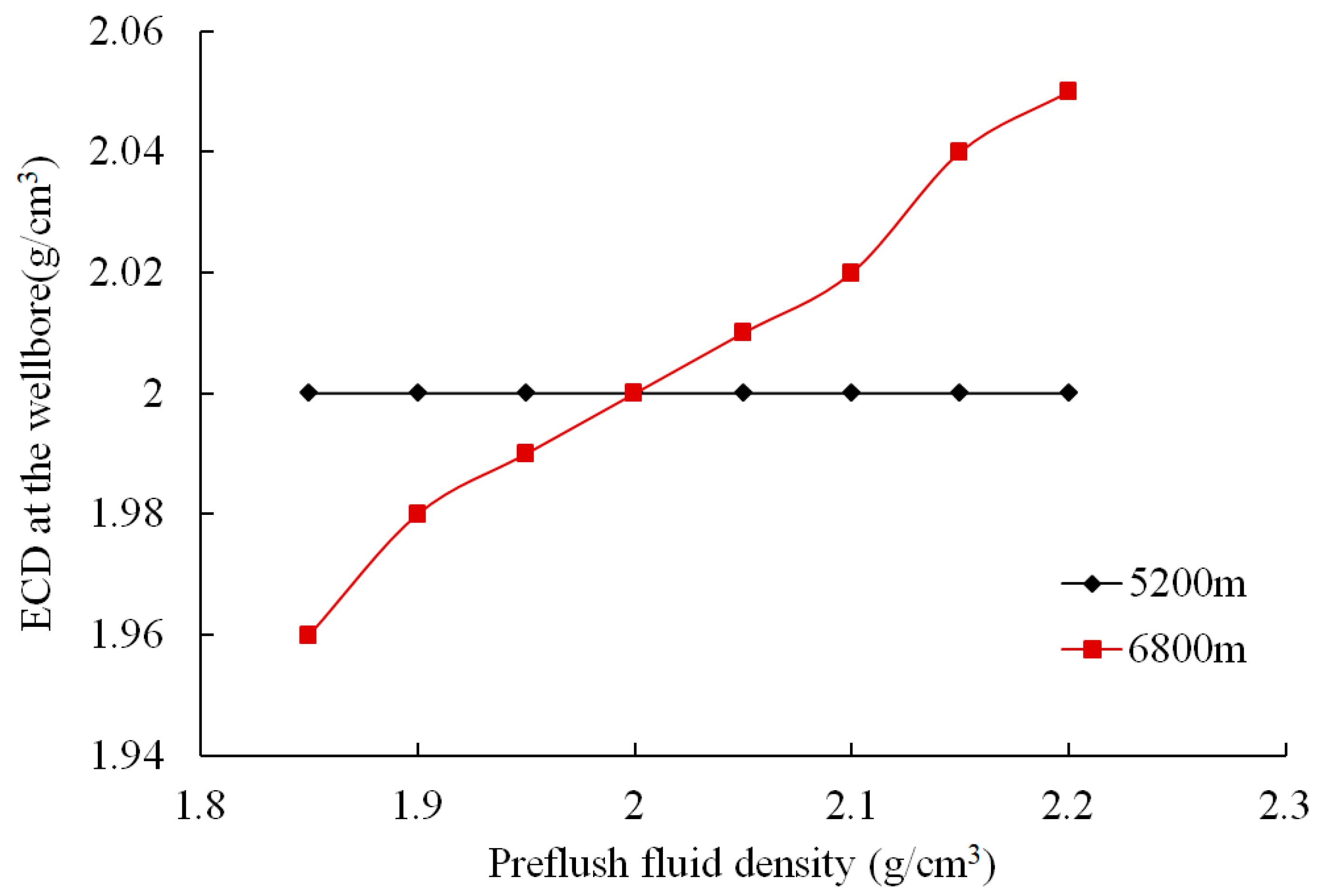
The densities of drilling fluid and cement slurry used in the well are 2.0 g/cm3 and 2.25 g/cm3. The cement return height and the preflush length are 4800 m and 400 m. For different preflush densities, ECDs at two key points were calculated for the critical phase of the pump shutdown and packer setting stage, as shown in Figure 8.
It can be seen from the figure that the pre-liquid density has no effect on the ECD at 5200 m, indicating that the pre-liquid did not return to the depth of the well during the pump shutdown and packer setting stage. With increase in the preflush density, the ECD at 6800 m increased. Since the pore pressure coefficient in the depth of the well reaches 2.1 g/cm3, in order to maintain the pressure balance in the depth of the well, combined with the actual requirements of the maximum annulus back-pressure of the MPC equipment of 7 MPa, according to the annulus back-pressure transfer model, the maximum value of back-pressure transmitted to the depth of the well is 3.56 MPa, then the density of the pre-liquid should be between 2.1–2.25 g/cm3. Considering the low-pressure layer at 5200 m, the density of the pre-liquid should be reduced as much as possible, so the density of the pre-liquid that should preferably be used is 2.1 g/ cm3.
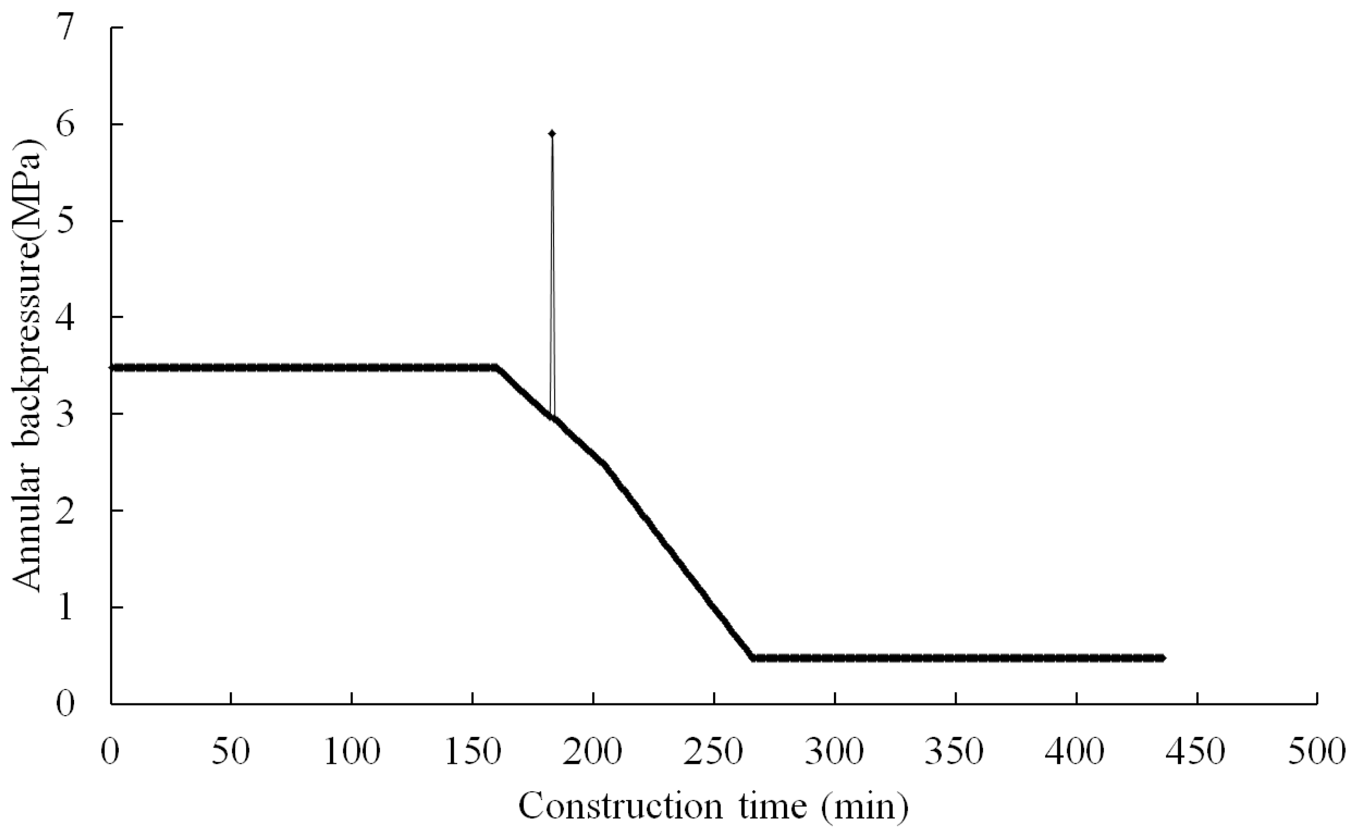
On this basis, the annulus back-pressure application value of the whole MPC process is calculated by using the above annulus back-pressure transfer model, as shown in Figure 9. Under this annulus back-pressure, the ECD at 5200 m and 6800 m was maintained at 2.05 g/cm3 and 2.12 g/cm3, respectively, and the MPC operation of the well was guided based on this result.

4. Conclusions

(1)
For the first time, a transient model of MPC annulus pressure wave propagation was established, coupling three non-Newtonian rheological models (Power-law, Bingham, and Herschel–Bulkley) for viscous dissipation with the elastic deformation of the casing-open-hole sections. It revealed the non-uniform attenuation characteristics of pressure waves in ultra-deep well annuli—slow attenuation in the casing sections, fast attenuation in the open-hole sections—and their flow–solid coupling mechanism, providing a directly usable theoretical tool for the precise design of MPC back-pressure compensation values in ultra-deep wells.
(2)
By comparing with the experimental data, the feasibility of the transient transmission model of pressure wave in annulus back-pressure is verified. The main influencing factors and influencing laws of pressure wave propagation in annulus fluid can be analyzed. The attenuation of the pressure wave is related to the fluid displacement and rheological mode of the annular fluid, and the larger the annulus fluid displacement, the more pressure wave attenuation. The attenuation laws of different rheological models are Power-law model > Herschel–Bulkley model > Bingham model. The attenuation value of pressure waves in multiple types of fluids is greater than that of single fluids.
(3)
The established pressure wave transient transmission model of annulus back-pressure provides theoretical support for the design and construction of on-site MPC.
(4)
Future research can proceed in the following directions: ① extend the model to gas–liquid–solid three-phase flow conditions to accommodate the analysis of annular pressure wave attenuation in gas-containing wells or under the impact of cuttings beds; ② combine real-time down-hole pressure monitoring data (PWD) to carry out online model calibration and dynamic parameter inversion studies; ③ generalize the one-dimensional model to analyze annular pressure wave attenuation in high-deviation and horizontal wells, introducing gravity component corrections for inclined and horizontal sections. In addition, the following limitations of the present study should be acknowledged. The field case analysis presented in Section 3.4 is based on a single well (Well XX-1), which limits the generalizability of the validation. Future work will focus on collecting additional field data from a broader range of ultra-deep wells to further validate the model across diverse geological and operational conditions. Furthermore, the present model is limited to single-phase liquid flow in the annulus; extension to gas–liquid two-phase or gas–liquid–solid three-phase conditions will be addressed in subsequent studies, as outlined in research direction ① above.
(5)
Computational efficiency and real-time implementation: the proposed model is primarily intended as an offline design tool for planning MPC operations. However, its computational efficiency is also relevant for potential real-time decision support during field execution. The computational time depends on the grid resolution and the total simulated duration. With the grid parameters specified in Section 2.3.1, a single simulation from pump shutdown to pressure stabilization can be completed on a standard workstation within a timescale that is well below the typical operational decision window (30–60 s) for pump shutdown and packer setting during MPC operations. This suggests that the model has the potential to support real-time decision-making. For applications requiring higher-frequency updates (≥1 Hz), the following strategy is proposed for future implementation: (i) offline generation of a training dataset covering the design parameter space using the full model; (ii) development of a reduced-order surrogate model using response surface methodology (RSM) or Gaussian process regression; (iii) real-time prediction using the surrogate model, calibrated periodically by the full model. This hybrid approach would enable sub-second response times while retaining the physical fidelity of the full model. It should be noted that implementation of the surrogate model is beyond the scope of the present study and is identified as a direction for future work.

Author Contributions

Conceptualization, J.Z.; Methodology, N.L., J.Z., L.Y., X.C., H.Y. and Q.G.; Software, N.L. and L.Y.; Validation, N.L., L.Y., X.C. and J.L.; Formal analysis, N.L., L.Y., X.C. and H.Y.; Investigation, N.L., J.Z., L.Y., X.C., H.Y., Q.G. and J.L.; Data curation, N.L., J.Z., L.Y., X.C., H.Y., Q.G. and J.L.; Writing—original draft, N.L.; Writing—review and editing, J.Z.; Supervision, J.Z.; Project administration, J.Z.; Funding acquisition, N.L. All authors have read and agreed to the published version of the manuscript.

Funding

This work was supported by the China National Petroleum Corporation Scientific and Technological Project (Grant No. 2023ZZ14YJ06) of “Research and Testing of Key Technologies for Ultra-Deep High-Temperature High-Pressure Well Drilling”, the National Science and Technology Major Project of “Intelligent Rig and Ultra-High Pressure Wellhead Equipment for 10,000-Meter Deep Wells” under Grant No. 2024ZD1401804 (Topic 4: 3000 hp Ultra-High Power Intelligent Cementing Equipment) and Grant No. 2024ZD1401802 (Topic 2: Key Equipment for 10,000-Meter Deep Drilling Including Intelligent Top Drive and Continuous Circulation System).

Data Availability Statement

The original contributions presented in this study are included in the article.

Conflicts of Interest

Authors Ning Li, Lvchao Yang, Heng Yang, and Jie Liang were employed by the Petrochina Tarim Oilfield Company. Authors Jingtian Zhang, Xiao Cai, and Qingfeng Guo were employed by the CNPC Engineering Technology R&D Company Limited. The remaining authors declare that the research was conducted in the absence of any commercial or financial relationships that could be construed as a potential conflict of interest.

Nomenclature

SymbolMeaningUnit
AAnnular flow cross-sectional aream2
d_hyAnnular hydraulic diameterm
EElastic modulusPa
gGravitational accelerationm/s2
HWell depthm
KConsistency coefficient (Power-law/Herschel–Bulkley models)Pa·sn
K_fFluid bulk modulus of elasticityPa
pPressurePa
R_iAnnular inner radius (outer radius of pipe string)m
R_oAnnular outer radius (borehole wall radius)m
tTimes
vFluid velocitym/s
zCoordinate along well depth directionm
γShear rates−1
μ_pPlastic viscosity (Bingham model)Pa·s
τ_0Yield stress (Bingham/Herschel–Bulkley models)Pa
τ_wWall shear stressPa
Abbreviations
AbbreviationFull name
ECDEquivalent Circulating Density
FDMFinite Difference Method
MOCMethod of Characteristics
MPCManaged Pressure Cementing

References

  1. Yang, H.; Li, J.; Zhang, Z.; Zhang, G.; Long, Z.; Zhang, H. A co-optimization method of equivalent circulating density and displacement efficiency in managed pressure cementing phase considering casing eccentricity. Phys. Fluids 2025, 37, 087181. [Google Scholar] [CrossRef] [Scilit]
  2. Zhou, X.J.; Liu, G.; Qiao, C.D.; Xia, L. Propagation of Pressure Waves in Viscous Fluids. Mech. Des. Manuf. 2013, 11, 50–52. [Google Scholar]
  3. Pierre, B. Pressure Waves in Pipelines and Impulse Pumping: Physical Principles, Model Development and Numerical Simulation. Ph.D. Thesis, Department of Petroleum Engineering and Applied Geophysics, Norwegian University of Science and Technology, Trondheim, Norway, December 2009. [Google Scholar]
  4. Li, X.; Ma, W.; Zhang, Z.; Chu, W. Study on Sound Wave Propagation of Hydrogen Pipeline Leakage Under 0 °C Low Temperature Conditions. Cryog. Supercond. 2024, 52, 86–92. [Google Scholar]
  5. Guo, X.J.; Cao, Z.; Xuan, B.W.; Deng, J.Q. Research on the Propagation Law of Pressure Waves in Leaking Pipelines. Water Resour. Hydropower Technol. 2021, 52, 94–104. [Google Scholar]
  6. Yang, Z.D.; Cao, Y.L.; Zhang, Q.L.; Zhao, S.M.; Cao, J.H.; Wu, F.; Li, G.D. Transient Flow Characteristics and Leakage Localization of Leaking Water Supply Pipelines. China Water Supply Drain. 2021, 37, 35–40. [Google Scholar]
  7. Chen, L. Study on the Impact of Viscoelastic Hybrid Pipeline Characteristics on Its Hydraulic Transient Dynamics. Ph.D. Thesis, Harbin Institute of Technology, Harbin, China, 2020. [Google Scholar]
  8. Yu, D. Overview of Methods for Handling Friction in Water Hammer Calculations. Hydropower Stn. Des. 2004, 2, 3–6. [Google Scholar]
  9. Yuan, H.; Niu, Z.; Huang, H.; Chen, W.; Chen, J.; Mu, X.; Lin, H. Study on transient flow characteristics of trapped air pockets at pipeline blind end impacted by water flow. Water Resour. Hydropower Eng. 2025, 1–15. Available online: https://sjwj.cbpt.cnki.net/portal/journal/portal/client/paper/a99a9cbd4b999e7def69181510a6735a (accessed on 26 July 2026).
  10. Wu, H.; Hu, X.X. Solving Transient Annulus System of Aero Engine Using Characteristic Line Method. J. Aerodyn. 2013, 28, 2003–2008. [Google Scholar]
  11. Shi, X.; Lü, H.X.; Zhu, D.L.; Sun, B.; Cao, B. Experiment and Numerical Simulation of Hydraulic Transient Condition of Branch Pipe Network. J. Drain. Irrig. Mech. Eng. 2013, 31, 406–412. [Google Scholar]
  12. Fu, X.; Yang, H.Y.; Bao, M.; Gao, H. Experimental Study and Numerical Simulation of Transient Phenomenon of Fluid Pressure in Hydraulic System. Mach. Tool Hydraul. 2000, 5, 13–14. [Google Scholar]
  13. Diao, X.; Shen, G.; Jiang, J.; Chen, Q.; Wang, Z.; Ni, L.; Mebarki, A.; Dou, Z. Leak detection and location in liquid pipelines by analyzing the first transient pressure wave with unsteady friction. J. Loss Prev. Process Ind. 2019, 60, 303–310. [Google Scholar] [CrossRef] [Scilit]
  14. Sondermann, C.N.; Viggiano, R.; de Freitas Rachid, F.B.; Bodstein, G.C.R. A Suitability Analysis of Transient One-Dimensional Two-Fluid Numerical Models for Simulating Two-Phase Gas-Liquid Flows Based on Benchmark Problems. Comput. Fluids 2021, 229, 105070. [Google Scholar] [CrossRef] [Scilit]
  15. Ding, L.; Ni, H. Transient fluctuation pressure during supercritical carbon dioxide drilling. Fault Block Oil Gas Field 2020, 27, 117–121. [Google Scholar]
  16. Sha, Y.; Wang, C.L.; Liu, T.; Shao, X.; Wen, J.L. Measurement and Hydraulic Calculation of Water Hammer Pressure Wave in Circular Tube Flow. J. Exp. Mech. 2007, 22, 527–533. [Google Scholar]
  17. Zhang, F.F.; Chen, J.W.; Li, B.X.; Zhao, C.; Zhang, S.Y.; Xiang, J.B.; Liu, Y.; Lou, W.Q. A Method for Solving Transient Pressure Fluctuations in Wellbores Based on Physics-Informed Neural Networks. Drill. Prod. Technol. 2026, 49, 153–159. [Google Scholar]
  18. Yan, T.; Qu, J.; Sun, X.; Chen, Y.; Pan, Y. Velocity and time law of back pressure pressure wave propagation in the wellbore of controlled pressure drilling. Nat. Gas Ind. 2017, 37, 77–84. [Google Scholar]
  19. Wang, X.Z.; Kong, X.W.; Wang, M.; Shen, J.W.; Fan, X.L.; Wang, X.D. Analysis of Influencing Factors of Pressure Control Drilling Gas and Drilling Fluid Two-Phase Pressure Decay. J. Appl. Mech. 2021, 38, 624–629. [Google Scholar]
  20. Yu, J.H.; Sun, N.; Liu, J. Analysis of the Response Time of Fine Pressure Control Drilling. Pet. Drill. Prod. Technol. 2011, 33, 20–24. [Google Scholar]
  21. Ding, S.D.; Liao, H.L.; Li, G.S.; Zhang, K.J. Analysis of Propagation Law of Wellhead Pulse Pressure in Annular Annulus. Nat. Gas Ind. 2007, 2, 57–59. [Google Scholar]
  22. Hou, C.; Tang, Y.; Zhuang, J.; Guo, Q.; Chu, X.; Miao, A.; Luo, S. Research on Pressure Optimization Control and Simulation of High-Pressure Tubing. J. Southwest Univ. 2021, 43, 130–137. [Google Scholar]
  23. Fan, H.H. (Ed.) Practical Drilling Fluid Mechanics; Petroleum Industry Press: Beijing, China, 2014. [Google Scholar]
  24. Mullins, L.D. Application of finite difference methods to analogue computational techniques. In Proceeding of the Rocky Mountain Annual Joint Meeting, Billings, MT, USA, 23–24 May 1957; SPE: Richardson, TX, USA, 1957; p. SPE-857-G. [Google Scholar]
  25. Von Rosenberg, D.U. Local Mesh Refinement for Finite Difference Methods. In Proceeding of the SPE Annual Technical Conference and Exhibition, New Orleans, LA, USA, 26–29 September 1982; SPE: Richardson, TX, USA, 1982; p. SPE-10974-MS. [Google Scholar]
  26. Mei, Y.T. Design and Simulation of Managed Pressure Cementing Operation in Offshore Wells with Narrow Pressure Window. Doctoral Dissertation, Yangtze University, Jingzhou, China, 2024. [Google Scholar] [CrossRef]
  27. Wen, P.; Wang, S.; Li, J.; Qu, R.; Li, T. Multiobjective optimization of a pressure maintaining ball valve structure based on RSM and NSGA-II. Sci. Rep. 2025, 15, 21342. [Google Scholar] [CrossRef] [Scilit] [PubMed]
  28. Zhou, H.; Liu, Z.; Shao, J.; Shen, W.; Essaieb, M. Effects of Stress Direction and Magnitude on Strength and Failure of Weakly Anisotropic Sandstone under True Triaxial Compression. Rock. Mech. Rock Eng. 2026, 59, 3213–3234. [Google Scholar]
  29. Lei, Z.; Dou, X.; Wang, Q.; Wang, R.; Ji, D.; Chen, Z.; Xing, G. A Semi-Analytical Model of a Hydraulically Fractured Horizontal Well with Pre-Darcy Flow and Stimulated Reservoir Volume in a Radial Composite Shale Reservoir. SPE J. 2025, 30, 743–761. [Google Scholar]
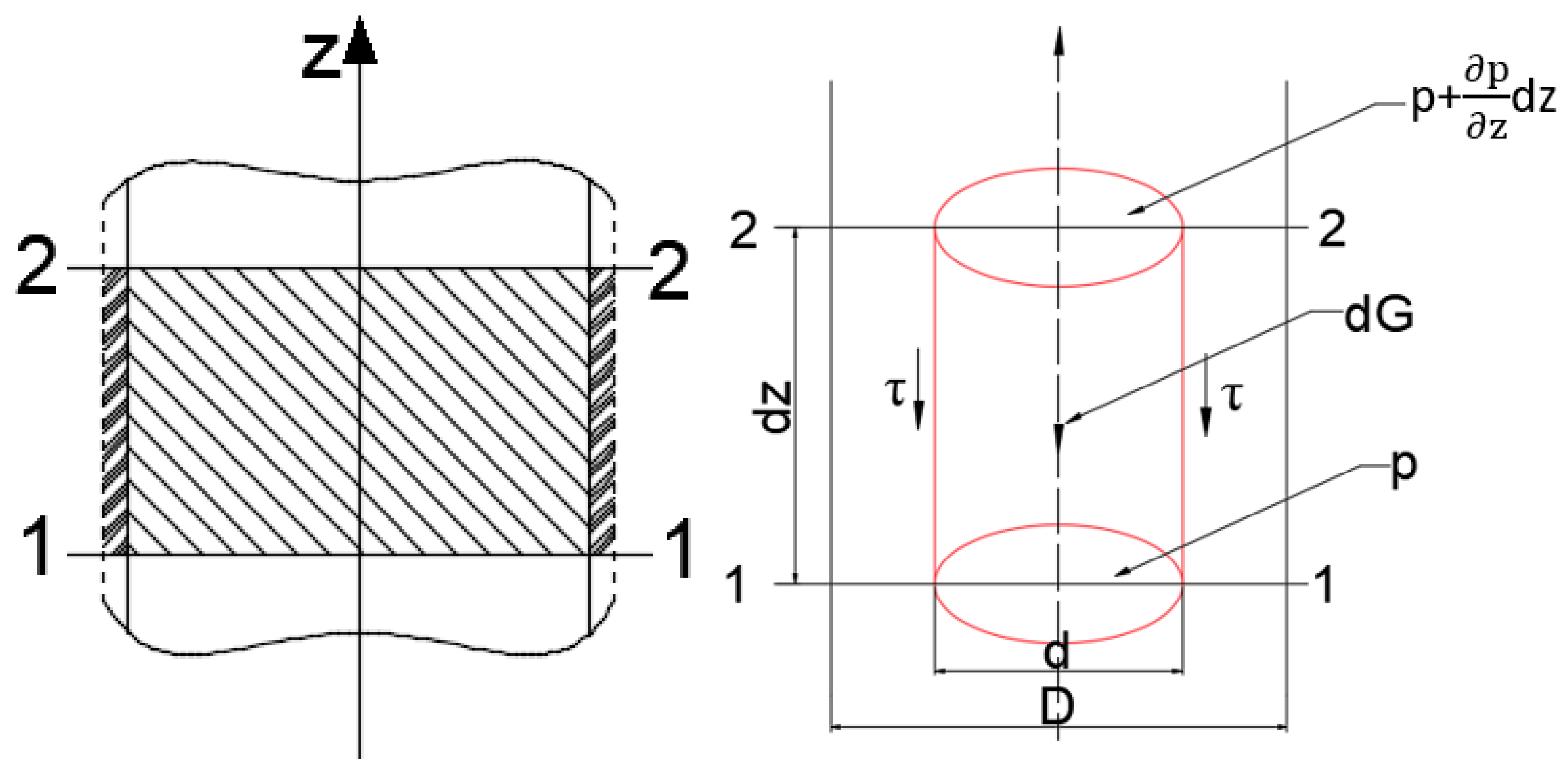
Figure 1. Schematic diagram of the forces on an annular fluid element (showing the position of the fluid element in the annulus and the direction of the forces).
Processes 14 02611 g001
Figure 2. Schematic of the finite difference discrete grid (showing the nodes and step sizes Δz and Δt in the time and space directions).
Processes 14 02611 g002
Figure 3. Schematic of the indoor pressure wave attenuation test setup (showing the high-pressure pump, nitrogen cylinder, pressure sensor locations, and a test section length of 20 m).
Processes 14 02611 g003
Figure 4. Annular back-pressure decay curves at different well depths (initial back-pressure 5 MPa, with the decay inflection point shown at a casing shoe depth of 5000 m).
Processes 14 02611 g004
Figure 5. Effect of the elastic modulus of the open-hole section rock (20–80 GPa) on bottom-hole pressure wave attenuation (initial back-pressure 5 MPa).
Processes 14 02611 g005
Figure 6. Results of bottom-hole pressure wave attenuation under different casing shoe depths (4000~6000 m) and formation elastic modulus (30~50 GPa) combinations.
Processes 14 02611 g006
Figure 7. Comparison curves of annular back-pressure decay along well depth under three rheological models (Power-law, Bingham, Herschel–Bulkley).
Processes 14 02611 g007
Figure 8. Effect of preflush fluid density in the pump-off sealing stage of Well XX-1 on the equivalent circulating density (ECD) at 5200 m and 6800 m.
Processes 14 02611 g008
Figure 9. Curve showing how the recommended annular back-pressure values for all MPC operations in Well XX-1 change over time/operation steps.
Processes 14 02611 g009
Table 1. The error between the calculation results and the experimental results.
Lab CodeBack-Pressure (MPa)Experimental Results (MPa)Calculation Results (MPa)Error (%)
132.822.742.8
22.52.362.216.4
321.891.757.4
41.51.381.305.8
510.920.942.2
Disclaimer/Publisher’s Note: The statements, opinions and data contained in all publications are solely those of the individual author(s) and contributor(s) and not of MDPI and/or the editor(s). MDPI and/or the editor(s) disclaim responsibility for any injury to people or property resulting from any ideas, methods, instructions or products referred to in the content.