Axial Flow Check Valve Flow-Field Simulation and Failure Analysis at the Compressor Outlet of a Gas Compressor Station

Abstract

In long-distance natural gas transmission, installing an axial flow check valve at the compressor outlet of a compressor station helps prevent backflow. Failure of this valve can cause compressor reverse rotation, which disrupts gas delivery. This study models and simulates the steady-state flow field at 100% valve opening and the transient flow features during valve opening and closing. In addition, a failed axial-flow check valve from a natural gas compressor station was disassembled, and initial observations of wear and deformation were used to verify the model. The results show that the maximum fluid velocity reaches 18.9 m/s at 100% valve opening, with a distinct vortex region forming in the throttling passage between the valve seat and disk. During valve opening, the inlet–outlet pressure difference decreases from 0.35 MPa at 0.001 s to 0.20 MPa at 0.080 s. At 60% relative opening, the maximum amplitude of the transient hydrodynamic force fluctuation reaches 662 N. During closure under a pressure difference of 300 kPa, the maximum disk velocity reaches 12.9 m/s. These transient flow and force characteristics, considered together with the wear observed on the guide sleeve and disk, provide insight into the delayed reseating of the valve.

1. Introduction

In long-distance natural gas transmission systems, booster stations must be installed at intervals to compensate for head loss and maintain transport capacity. As a critical protection component at the compressor outlet, the axial flow check valve prevents reverse flow and reduces the risk of compressor reverse rotation, which is essential for pipeline safety [1,2,3,4]. However, due to complex flow field effects, wear of mechanical components, and fluctuations in operating conditions, axial flow check valves are prone to malfunctions such as failure to reseat properly [5,6,7,8]. Once failure occurs, the compressor may require shutdown and maintenance, and the resulting pressure fluctuations can cause supply interruptions and secondary risks, leading to substantial economic losses [9,10,11,12,13]. Therefore, clarifying the internal flow field characteristics and failure mechanisms of axial flow check valves is of considerable theoretical and practical value for optimizing valve design and improving operating reliability.

Previous studies have examined valve opening, force balance, impact response, and structural stability from complementary perspectives. Wu et al. [14] performed dynamic-valve simulations and established a predictive relationship between the medium flow rate and disk opening. Botros [15] identified spring stiffness as a governing design parameter and showed that an imbalance between the hydrodynamic and spring forces can prevent full opening and promote disk vibration. Wang et al. [16] evaluated collision-induced stresses in an oil well pump valve, while Sun [17] investigated check valve core stability using a fluid–structure interaction framework. Nilsson et al. [18] employed finite element analysis to evaluate impact stresses in flapper valves. Himr et al. [19,20] experimentally examined check valve behavior during pump trip and analyzed valve slam in a pumping station, demonstrating the close relationship between valve motion and pipeline transients. Transient CFD research has progressively developed from prescribed valve motion toward dynamically coupled disk response and experimental validation. Li et al. [21] used a dynamic mesh and user-defined function to simulate the transient behavior of a swing check valve. Zhang et al. [22] analyzed disk acceleration and valve-seat loading during axial flow check valve closure, while Zhang et al. [23] examined the stress evolution of the disk during the closing process. Wang et al. [24] modeled the instantaneous collision between the disk and valve seat. Li et al. [25] analyzed the internal flow field of a low-flow-resistance axial flow check valve, whereas other CFD studies investigated spring-loaded valve reclosure, check-valve dynamics, and CFD-based design validation [26,27,28]. Recent efforts have further addressed damping during axial flow check valve closure [29], fluid–structure-interaction-induced vibration in sleeve control valves [30], experimentally validated nozzle-check-valve dynamics and fluid–valve transient interaction [31], transient fluid–structure interaction in high-pressure hydrogen decompression valves [32], and impact–wear behavior of valve–seat pairs [33]. These studies demonstrate the increasing emphasis on coupled transient, structural, and experimentally supported analyses.

Despite these advances, previous studies have mainly focused on flow characteristics, disk motion, closing impact, or structural response under numerical or laboratory conditions. The connection between these analyses and a documented in-service failure at a compressor station has received less attention. The present study addresses this gap through a case study of an axial-flow check valve that failed to reseat at a natural gas compressor outlet. A three-dimensional model was established from measurements of the actual valve, and the flow field at 100% opening and the transient opening and closing processes were investigated. The pressure and velocity fields, disk motion, and hydrodynamic force characteristics were analyzed. These numerical results were then considered together with the wear observed during disassembly of the same valve to examine the possible relationship between internal flow behavior and delayed reseating. The contribution of this study therefore lies in combining steady and transient CFD analyses with evidence from an actual valve failure case.

2. Flow Field Simulation of the Axial Flow Check Valve in a Compressor Station

2.1. Valve Structure and Operating Principle

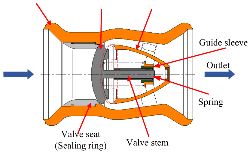
The principal components of an axial flow check valve include the valve body, disk, spring, guide sleeve, and sealing ring [34]. During opening, fluid pressure drives the disk to move linearly along the axial guide mechanism, forming a flow passage. When flow stagnates or reverses, the spring preload pushes the disk back to its closed position. A three-dimensional model was constructed based on measurements of the actual valve. The structure of the axial flow check valve is shown in Figure 1.

2.2. Mathematical Model for Three-Dimensional CFD Simulation

2.2.1. Governing Equations for the Three-Dimensional CFD Simulation

The continuity equation is:

$${\displaystyle \frac{\partial \rho }{\partial t}}+{\displaystyle \frac{\partial (\rho u_i)}{\partial x_i}}=0$$

(1)

The momentum equation is:

$${\displaystyle \frac{\partial (\rho u_i)}{\partial t}}+{\displaystyle \frac{\partial (\rho u_i{u}_j)}{\partial x_j}}=-{\displaystyle \frac{\partial p}{\partial x_i}}+{\displaystyle \frac{\partial {\tau }_{ij}}{\partial x_j}}$$

(2)

The energy equation is:

$${\displaystyle \frac{\partial (\rho E)}{\partial t}}+\nabla \cdot [u(\rho E+p)]=\nabla \cdot [\lambda \nabla T+(\tau \cdot u)]$$

(3)

where $\rho$ is the local gas density, kg/m³; $t$ is time, s; $u_i$ and $u_j$ are the Reynolds-averaged velocity components in the i and j directions, respectively, m/s; x_i and x_j are the corresponding Cartesian coordinates, m; p is the static pressure, Pa; and ${\tau }_{ij}$ is the effective stress tensor incorporating the molecular and modeled turbulent stresses, Pa. Moreover, u is the velocity vector, m/s; E is the total specific energy, J/kg; T is the absolute temperature, K; and $\lambda$ is the effective thermal conductivity incorporating both molecular and turbulent heat transport, W/(m·K).

2.2.2. Turbulence Model

The standard $k-\epsilon$ Reynolds-averaged turbulence model was used in all steady and transient simulations. This model was selected for its robustness in industrial internal-flow and dynamic-mesh calculations. Standard wall functions were employed for near-wall treatment. The transport equations for turbulent kinetic energy $k$ and its dissipation rate $\epsilon$ are:

$${\displaystyle \frac{\partial (\rho k)}{\partial t}}+{\displaystyle \frac{\partial (\rho k{u}_j)}{\partial x_j}}={\displaystyle \frac{\partial }{\partial x_j}}\left[\left(\mu +{\displaystyle \frac{{\mu }_t}{{\sigma }_k}}\right){\displaystyle \frac{\partial k}{\partial x_j}}\right]+G_k-\rho \epsilon$$

(4)

$${\displaystyle \frac{\partial (\rho \epsilon )}{\partial t}}+{\displaystyle \frac{\partial (\rho \epsilon u_j)}{\partial x_j}}={\displaystyle \frac{\partial }{\partial x_j}}\left[\left(\mu +{\displaystyle \frac{{\mu }_t}{{\sigma }_{\epsilon }}}\right){\displaystyle \frac{\partial \epsilon }{\partial x_j}}\right]+C_{1\epsilon }{\displaystyle \frac{\epsilon }{k}}{G}_k-C_{2\epsilon }\rho {\displaystyle \frac{{\epsilon }^2}{k}}$$

(5)

where the production of turbulent kinetic energy is:

$$G_k={\mu }_t\left({\displaystyle \frac{\partial u_i}{\partial x_j}}+{\displaystyle \frac{\partial u_j}{\partial x_i}}\right){\displaystyle \frac{\partial u_i}{\partial x_j}}$$

(6)

and the turbulent viscosity is:

$${\mu }_t=\rho C_{\mu }{\displaystyle \frac{k^2}{\epsilon }}$$

(7)

where k is the turbulent kinetic energy, m²/s²; $\epsilon$ is its dissipation rate, m²/s³; $\mu$ is the molecular dynamic viscosity, Pa·s; ${\mu }_t$ is the turbulent viscosity, Pa·s; and Gk is the production of turbulent kinetic energy, kg/(m·s³). The model constants were $C_{\mu }$ = 0.09, $C_{1\epsilon }$ = 1.44, $C_{2\epsilon }$ = 1.92, ${\sigma }_k$ = 1.0, ${\sigma }_{\epsilon }$ = 1.3.

2.2.3. Mathematical Model of Disk Motion

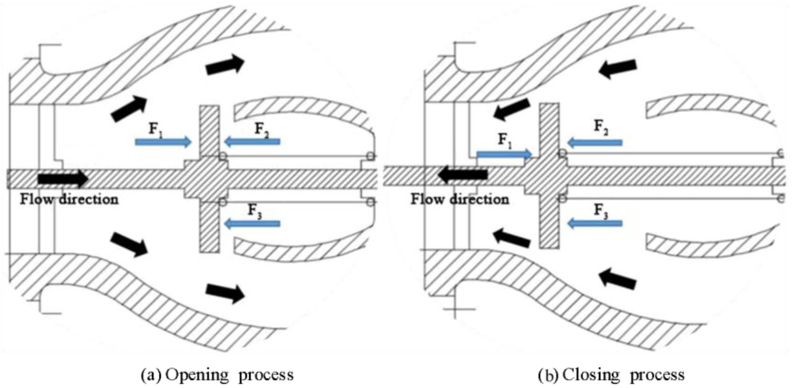
Based on the operating principle, only axial forces on the disk are considered. The net axial force acting on the disk is (Figure 2):

$${\displaystyle \sum F}=F_1-F_2-F_3$$

(8)

$$F_3=k_s\cdot (x_0+x)$$

(9)

where F₁ and F₂ are the fluid forces on the two sides of the disk, N; F₃ is the spring force, N; x₀ is the minimum spring compression at full closure, m; x is the axial displacement of the disk to the right (x = 0 when fully closed), m; and k_s is the spring stiffness, N/m.

The differential equation of motion is derived from Newton’s second law:

$$m{\displaystyle \frac{d^{2}x}{d{t}^2}}={\displaystyle \sum F}$$

(10)

where m is the disk mass, kg; and t is time, s.

The differential form of the momentum theorem is:

$${\displaystyle \sum F}={\displaystyle \frac{d(mv)}{dt}}$$

(11)

The velocity and displacement increments are:

$${\displaystyle \frac{dv}{dt}}={\displaystyle \frac{v_{i+1}-v_i}{\Delta t}}$$

(12)

$${\displaystyle \frac{dx}{dt}}={\displaystyle \frac{x_{i+1}-x_i}{\Delta t}}$$

(13)

where v_i and v_i+1 are disk velocities at times t_i and t_i+1, m/s; x_i and x_i+1 are displacements, m; and $\Delta t$ is the time-step size.

From the differential equation of a particle and the momentum theorem, we obtain:

$$v_{i+1}=v_i+{\displaystyle \frac{{\displaystyle \sum F\cdot \Delta t}}{m}}$$

(14)

$$x_{i+1}=x_i+{\displaystyle {\int }_{t_i}^{t_{i+1}}v(t)dt}$$

(15)

2.2.4. Flow Passage Model Construction

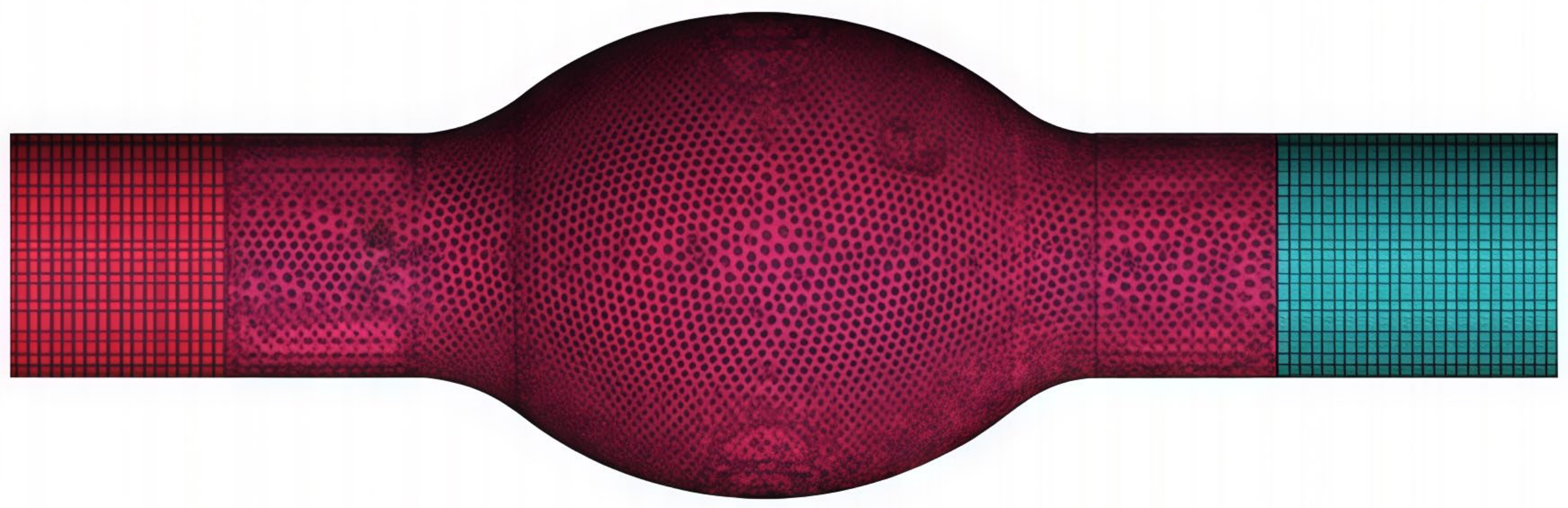
The flow passage model was extracted from the product geometry. According to national standards, the inlet and outlet pipe lengths are set to five and ten times the nominal diameter to ensure full development of the flow. The three-dimensional flow-passage model is shown in Figure 3, and the mesh configuration is shown in Figure 4.

2.2.5. Boundary Conditions and Parameter Settings

Natural gas at 293 K was used as the working medium. The absolute operating pressure for the main valve simulations was set to 8 MPa, based on the ideal gas eq temperature using the ideal gas equation of state. The energy equation was enabled to account for temperature variation and its effect on gas density. The thermophysical properties used in the calculations are listed in

Table 1. Thermophysical properties of natural gas used in the numerical calculations.

Temperature (K)	Reference Density at 293 K and 8 MPa (kg/m3)	Viscosity (kg/m·s)	Specific Heat (J/kg·K)	Thermal Conductivity (W/m·K)	Molecular Weight (kg/kmol)
293	55.8	1.0 × 10−5	2100	0.033	17

.

All pressures specified for the main valve calculations are gauge pressures relative to the absolute operating pressure of 8 MPa. Thus, a gauge pressure of 0 kPa corresponds to an absolute pressure of 8 MPa rather than a vacuum condition. Because the flow direction reverses during valve closure, the two ends of the computational domain are identified according to their fixed physical locations as the compressor-side boundary and the pipeline-side boundary. The boundary and initial conditions used for the different simulation cases are summarized in

Table 2. Boundary and initial conditions used for the different simulation cases.

Simulation Case	Initial Disk Condition	Compressor-Side Boundary	Pipeline-Side Boundary	Temporal Condition
Experimental validation	Fixed at 100% opening	Mass flow inlet corresponding to the measured volumetric flow rates of 230–480 m3/h	Static pressure outlet: 0 kPa	Steady
Full-open steady state	Fixed at 100% opening	Total pressure inlet: 150 kPa	Static pressure outlet: 0 kPa	Constant
Transient opening	Fully closed; initial velocity of 0 m/s	Mass flow inlet: 0–30 kg/s	Static pressure outlet: 0 kPa	Linear increase during 0–0.08 s, followed by a constant value.
Transient closing	Fully open; initial velocity of 0 m/s	Static pressure outlet: 0 kPa	Total pressure inlet: 100, 200, or 300 kPa	Linear increase from 0 to the specified pressure during 0–0.005 s, followed by a constant value

.

For the experimental validation calculations, the measured volumetric flow rates were converted into mass-flow rates using the gas density at the experimental pressure and temperature. The measured flow rate was prescribed, while the pressure drop was retained as an independent CFD output. The opening calculation was initialized from a converged zero-flow solution with the disk fully closed, whereas the closing calculations were initialized from the corresponding fully open steady-state solution. The 200 kPa closing condition was used for the grid- and time-step-sensitivity assessments.

All stationary surfaces were treated as hydraulically smooth, no-slip, adiabatic walls. The disk was defined as a no-slip moving wall constrained to axial translation, with the remaining degrees of freedom fixed. Its spring force was calculated using the motion equation in Section 2.2.3. Gravity was neglected because the valve axis was horizontal. At the inflow boundaries, the gas temperature, turbulence intensity, and hydraulic diameter were set to 293 K, 5%, and 0.20 m, respectively. The same values were specified for possible backflow at the pressure outlets.

A three-dimensional, double-precision, pressure-based solver was selected because the operating conditions corresponded to low-Mach-number internal flow; the calculated maximum local velocity of 23.1 m/s (Ma < 0.06) confirmed this flow regime. Double precision was used to resolve pressure and force variations that were small relative to the absolute operating pressure of 8 MPa. The standard k–ε model with standard wall functions was adopted, and the energy equation was enabled to account for pressure- and temperature-dependent gas density. Pressure was interpolated using a second-order scheme, while the momentum, k, ε, and energy equations were discretized using second-order upwind schemes to reduce numerical diffusion in the throttling and recirculation regions. SIMPLE was used for pressure–velocity coupling. The residual limits were 1 × 10⁻⁵ for continuity, momentum, k, and ε, and 1 × 10⁻⁶ for energy, with a maximum of 50 iterations per time step. Hydrodynamic force and disk displacement were also monitored to confirm convergence.

2.2.6. Mesh Generation and Grid- and Time-Step-Sensitivity Assessment

A hybrid meshing strategy was adopted for the computational domain. The inlet and outlet pipes were discretized using hexahedral elements, whereas tetrahedral elements were used in the valve flow passage because of its geometric complexity. Local mesh refinement was applied around the disk, valve seat, and throttling region, where large pressure and velocity gradients were expected. The resulting mesh is shown in Figure 4.

Both spatial and temporal discretization may affect the calculated flow field and disk motion during valve opening and closing. Therefore, grid- and time-step-sensitivity assessments were conducted before the subsequent simulations. The closing time was defined as the interval from the initiation of the prescribed reverse-flow condition to the instant at which the disk reached the closed position. The closing velocity was defined as the axial velocity of the disk immediately before it reached the closed position.

For the grid-sensitivity assessment, three meshes containing 693,084, 853,052, and 1,035,486 elements were examined under the same transient closing condition at a pressure difference of 0.2 MPa. The same boundary conditions, convergence criteria, dynamic-mesh settings, and time step were applied to all three meshes. To minimize the influence of temporal discretization on the grid comparison, the smallest tested time step of 0.00001 s was used for all three grid cases. The closing velocity and closing time were selected as the monitored quantities. The results are summarized in

Table 3. Grid independence test for the flow passage of the axial flow check valve.

Mesh Type	Node Count	Element Count	Closing Velocity (m/s)	Closing Time (s)
Mesh 1	1,562,304	693,084	10.9151	0.0322
Mesh 2	2,135,786	853,052	10.8351	0.0299
Mesh 3	2,864,375	1,035,486	10.8260	0.0292

.

The changes between two successive mesh levels were evaluated to determine whether the calculated disk response approached a grid-stable range. When the number of elements increased from 693,084 in Mesh 1 to 853,052 in Mesh 2, the closing velocity and closing time changed by 0.74% and 7.69%, respectively. A further increase to 1,035,486 elements in Mesh 3 resulted in changes of only 0.08% in the closing velocity and 2.40% in the closing time.

The substantially smaller changes observed during the second refinement indicate that the calculated disk response approached a stable range. Increasing the element count from Mesh 2 to Mesh 3 by 21.4% produced only a minor change in the closing velocity, while the change in closing time was markedly smaller than that observed between Mesh 1 and Mesh 2. In addition, Mesh 2 contained 17.6% fewer elements than Mesh 3. Therefore, Mesh 2 was selected for the subsequent steady and transient simulations as a balance between spatial resolution and computational cost.

After the grid-sensitivity assessment, the effect of the time-step size was examined using Mesh 2. Three time steps were tested under the same transient closing condition at a pressure difference of 0.2 MPa. The boundary conditions, convergence criteria, spatial-discretization schemes, and dynamic-mesh settings were kept unchanged. The closing velocity and closing time were again used as the monitored quantities. The results are presented in

Table 4. Time-step sensitivity results for the transient closing process.

Case	Time Step (s)	Closing Velocity (m/s)	Closing Time (s)
Case 1	0.002	10.6752	0.0224
Case 2	0.001	10.8367	0.0281
Case 3	0.00001	10.8396	0.0284

.

The changes between successive time-step cases were compared to evaluate the sensitivity of the calculated disk response to temporal discretization. When the time step was reduced from 0.002 s to 0.001 s, the closing velocity and closing time changed by 1.49% and 20.28%, respectively. When the time step was further reduced by two orders of magnitude to 0.00001 s, the corresponding changes decreased to 0.03% and 1.06%.

The substantially smaller changes obtained after the second reduction indicate that the calculated closing velocity and closing time approached a time-step-stable range. Reducing the time step from 0.001 s to 0.00001 s requires approximately one hundred times more time steps for the same simulated duration but produces only minor changes in the monitored quantities. Therefore, a time step of 0.001 s was selected for the subsequent transient simulations as a balance between temporal resolution and computational cost.

Based on the grid- and time-step-sensitivity assessments, Mesh 2 and a time step of 0.001 s were used for all subsequent transient simulations.

2.3. Dynamic-Mesh Formulation and Numerical Implementationl

2.3.1. Dynamic Mesh Mathematical Model

The mesh is updated automatically at each time increment according to boundary displacements. The conservation equation is:

$${\displaystyle \frac{d}{dt}}{\displaystyle {\int }_V\rho \varphi dV}+{\displaystyle {\int }_{\partial V}\rho \varphi (u-u_g)\cdot dA}={\displaystyle {\int }_{\partial V}\Gamma \nabla \varphi \cdot dA}+{\displaystyle {\int }_V{S}_{\varphi }dV}$$

(16)

where $\rho$ is the fluid density; $\varphi$ is a generic transported scalar; $u$ is the fluid velocity vector; $u_g$ is the grid-velocity vector; $\Gamma$ is the diffusion coefficient associated with $\varphi$; $S_{\varphi }$ is the source term; $V$ is the moving control volume; $\partial V$ is its boundary; $dV$ is the differential volume element; and $dV$ is the outward differential area vector.

Using a first-order backward differencing scheme, the temporal derivative becomes:

$${\displaystyle \frac{d}{dt}}{\displaystyle {\int }_V\rho \varphi dV}={\displaystyle \frac{{(\rho \varphi V)}^{n+1}-{(\rho \varphi V)}^n}{\Delta t}}$$

(17)

where the superscripts n and n + 1 denote the current and next time levels.

The control volume Vⁿ⁺¹ at time step n + 1 is:

$$V^{n+1}=V^n+{\displaystyle \frac{dV}{dt}}\Delta t$$

(18)

To satisfy the conservation of mesh volume, the time derivative of the control volume is:

$${\displaystyle \frac{dV}{dt}}={\displaystyle {\int }_{\partial V}{u}_g}\cdot dA={\displaystyle {\displaystyle \sum _j^{N_f}}{u}_{g,j}}\cdot A_j$$

(19)

where N_f is the number of faces of the control volume, u_g,j is the grid velocity at face j, and A_j is its area vector. For each face:

$$u_{g,j}\cdot A_j={\displaystyle \frac{\delta V_j}{\Delta t}}$$

(20)

where $\delta V_j$ is the volume swept by face j during the time interval $\Delta t$.

2.3.2. Dynamic Mesh Method and Parameter Settings

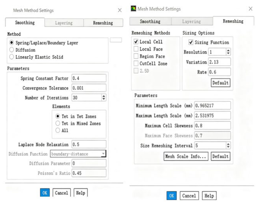
The disk surface was defined as a rigid moving boundary, the surrounding tetrahedral fluid zone as a deforming zone, and the remaining walls as stationary boundaries. As shown in Figure 5, the Spring/Laplace/Boundary Layer smoothing method was used with a spring constant factor of 0.4, a convergence tolerance of 0.001, and a maximum of 30 iterations. Local cell remeshing was enabled with cell-length limits of 0.965–2.531 mm, a maximum cell skewness of 0.8, and a remeshing interval of 5 to prevent excessive mesh distortion during disk motion.

2.3.3. UDF-Based Disk Motion Implementation

The disk motion was implemented using a compiled UDF based on the DEFINE_CG_MOTION macro. At each time step, the axial pressure force and spring restoring force were used to calculate the disk acceleration, velocity, and displacement according to Equations (9), (10), (14), and (15). Only axial translation was permitted, while the transverse and rotational motions were constrained. The resulting disk velocity was transferred to the dynamic-mesh module, where mesh smoothing and local remeshing were performed using the settings shown in Figure 5. Disk travel was limited to the physical interval between the fully closed and fully open positions.

2.4. CFD Model Validation

To validate the CFD model, steady-state pressure-drop measurements were conducted on the axial flow check valve investigated in this study. The pressure drop was determined from the difference between the pressures measured at the upstream and downstream sections of the valve. Corresponding CFD calculations were performed at the measured volumetric flow rates using the same valve geometry, opening position, working medium, and operating conditions as those employed in the experiments.

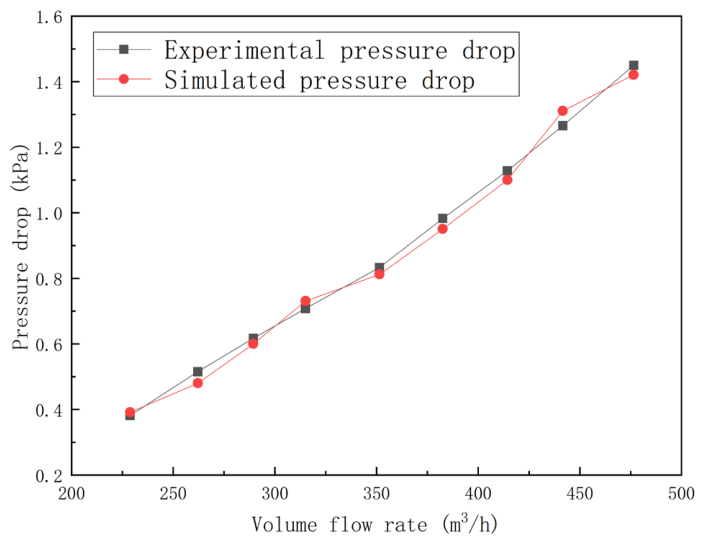
Figure 6 compares the calculated pressure drops with the experimental measurements. The pressure drop increases continuously with increasing volumetric flow rate, and the numerical results reproduce the variation observed in the experiments. The two curves remain close throughout the investigated flow rate range, with only small discrepancies at several intermediate flow rates. This agreement indicates that the adopted CFD model can reasonably predict the steady-state pressure-loss characteristics of the axial-flow check valve and provides support for the subsequent flow-field analysis.

3. Flow-Field Simulation and Failure Analysis of the Axial Flow Check Valve

3.1. Pressure and Velocity Characteristics Under Steady-State Flow at 100% Opening

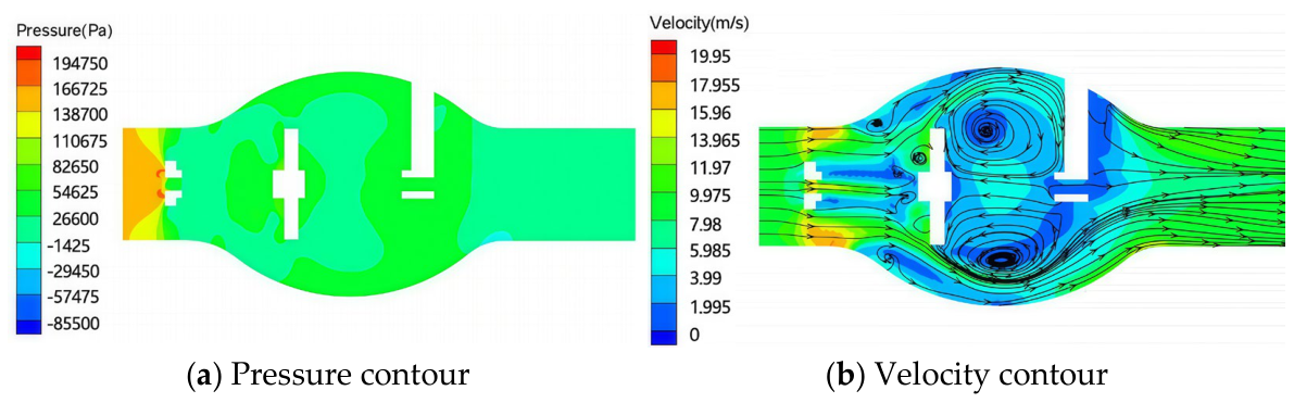
Using FLUENT, a numerical model of the failed axial flow check valve was constructed to simulate the steady-state pressure and velocity fields at 100% opening. The inlet pressure is set to 150 kPa and the outlet pressure to 0. The resulting pressure and velocity distributions are shown in Figure 7; they indicate that the internal flow field exhibits complex hydrodynamic behavior at full opening. When the medium enters the throttling region between the valve seat and the disk, the abrupt reduction in cross-sectional area produces significant velocity variation. The maximum velocity reaches 18.9 m/s. These rapid changes in velocity generate a distinct vortex region within the throttling region, which reflects energy loss as the fluid passes through this area. The presence of the vortex increases turbulence intensity and may induce local pressure fluctuations that affect valve performance. The pressure-gradient distribution shows that the pressure peak is concentrated near the inlet. As the flow enters this region, the sudden contraction of the passage and the deflection of the flow trajectory convert kinetic energy into pressure energy, forming a local high-pressure zone. Downstream of the throttling element, the streamlines become nonuniform, pressure decreases markedly, and velocity rises. This combined decrease in pressure and increase in velocity reflects the flow-acceleration effect induced by the throttling geometry and the flow passage’s shape. The highest velocities occur primarily at the interface between the throttling element and the valve body, where the flow area is smallest and the fluid is forced to accelerate, forming a high-speed jet region.

3.2. Pressure and Velocity Characteristics During Valve Opening

3.2.1. Pressure Distribution During the Opening Process

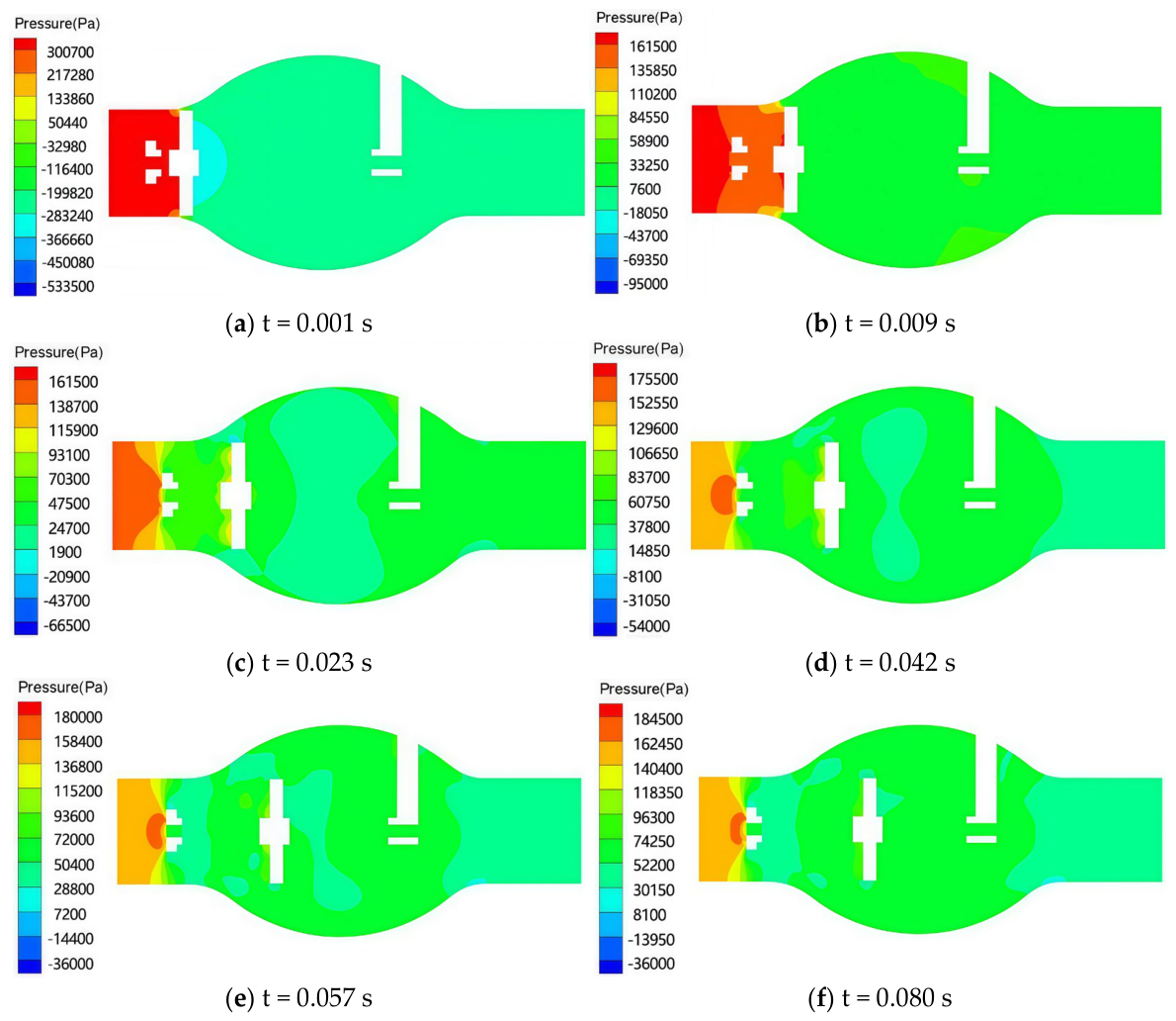
Figure 8 presents the pressure contours within the valve domain at different times during the opening process. Analysis of these contours provides insight into the hydrodynamic behavior at various opening positions and its effect on system performance. At t = 0.001 s, the opening is minimal, allowing only a small portion of the fluid to exit through the outlet. This restricted flow produces a pronounced pressure difference of up to 0.35 MPa between the inlet and outlet. A stable high-pressure region forms at the inlet. After the fluid passes the disk, the pressure drops sharply and negative-pressure zones appear within the valve chamber and near the outlet. Figure 8b–d shows the pressure evolution from t = 0.009 s to 0.042 s. During this period, the disk is driven rightward by the fluid, gradually enlarging the opening. This expansion releases the previously constrained pressure, and stratification of the pressure field becomes more evident. The pressure in the central valve chamber increases progressively, whereas the inlet–outlet pressure difference decreases. At t = 0.023 s and t = 0.042 s, the inlet–outlet pressure differences are 0.24 MPa and 0.22 MPa, respectively. Figure 8e,f shows the pressure contours at t = 0.057 s and 0.080 s, representing the late stage of opening. The flow becomes increasingly stable, and the inlet–outlet pressure difference continues to decrease, with the pressure field approaching steady-state conditions. At these times, the pressure differences are 0.21 MPa and 0.20 MPa, respectively.

3.2.2. Velocity Distribution During the Opening Process

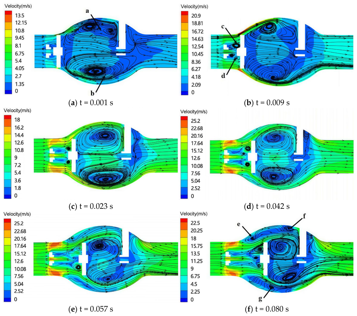
Figure 9 shows the velocity contours within the valve domain at different times during valve opening. At t = 0.001 s (Figure 9a), the opening is small, allowing only a narrow jet of fluid to pass through the slit between the disk and the flow passage. A high-velocity region forms along the disk edge, with a maximum velocity of 12 m/s. The inlet, outlet, and valve chamber show low velocities of approximately 1 m/s. As the fluid passes the disk, flow disturbance occurs and vortices form inside the chamber, as indicated at positions a and b. These vortices cause additional energy loss and further disturb the local flow field, which may affect disk motion. At t = 0.009 s (Figure 9b), the high-velocity region remains concentrated near the disk, with a maximum velocity of 20 m/s. Compared with the earlier stage, this high-speed area expands, and small vortices form on the left side of the disk, as shown at positions c and d. These vortices further affect disk motion. From t = 0.023 s to 0.057 s (Figure 9c–e), as the valve continues to open, a larger volume of fluid flows through the chamber, driving the disk to move axially to the right. Velocities within the chamber and at the outlet increase steadily. The vortices at positions a and b shrink, and flow speeds within the vortex regions remain low. At t = 0.080 s (Figure 9f), the valve is fully open. New small vortices appear along the outer edges of the chamber at positions e, f, and g, and the maximum velocity reaches 22.5 m/s.

3.2.3. Comparison of Hydrodynamic Forces During Valve Opening

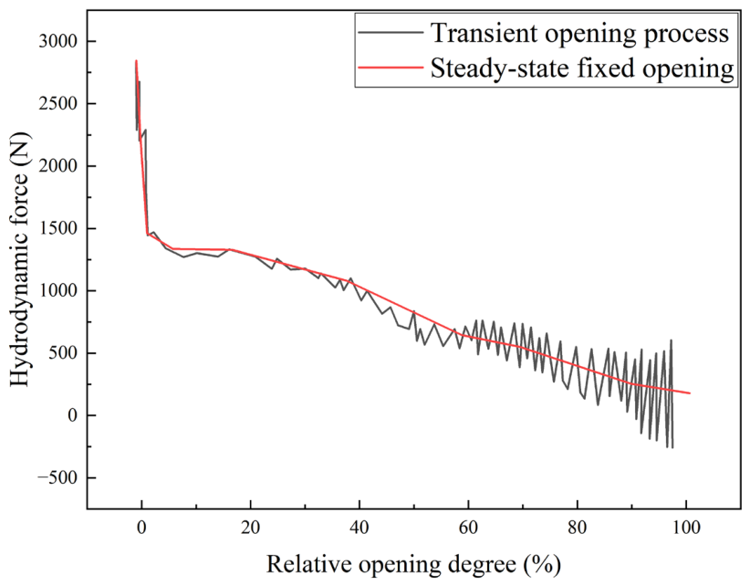
Figure 10 compares steady-state and transient hydrodynamic forces during valve opening. The hydrodynamic force decreases overall as the opening increases. At the same time, the magnitude of transient-force fluctuations increases with opening. When the valve reaches 60% relative opening, the transient-force fluctuation becomes pronounced, with a maximum amplitude of 662 N. This behavior occurs because, during transient opening, the disk moves with finite acceleration. Pressure fluctuations inside the valve cause the disk to oscillate, generating fluctuations in transient hydrodynamic force.

3.3. Pressure and Velocity Characteristics During Valve Closure

3.3.1. Pressure Distribution During the Closing Process

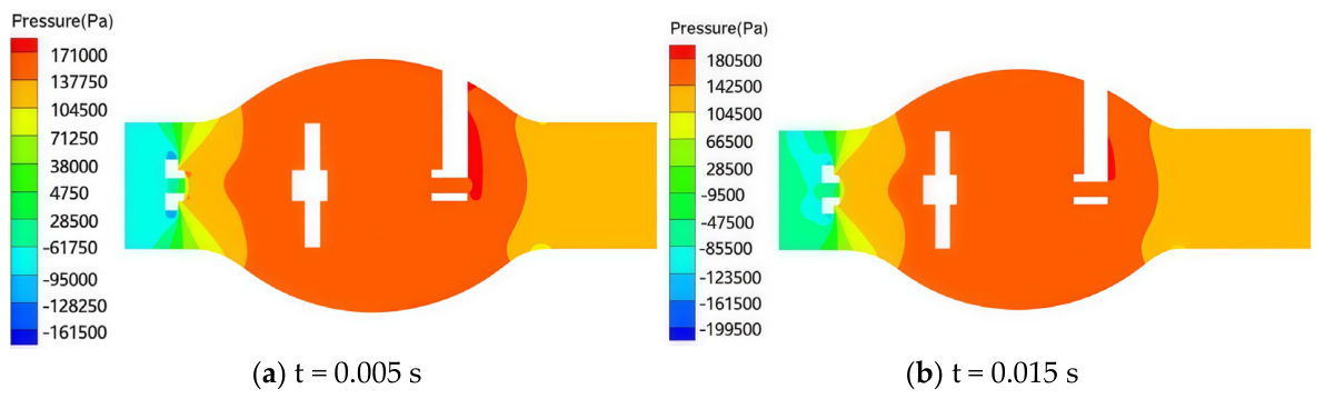
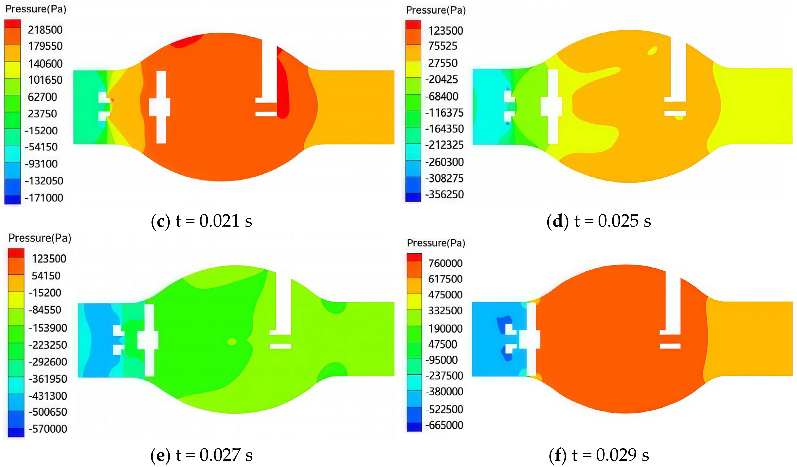
Figure 11 shows the pressure contours within the valve domain at different time steps during the closing process. At t = 0.005 s (Figure 11a), the valve is in the initial stage of closing. The pressure distribution inside the chamber is relatively uniform, with the high-pressure region concentrated within the chamber. The maximum pressure reaches 0.17 MPa. After passing the disk, the fluid experiences a gradual pressure decrease, and the inlet–outlet pressure difference is 0.12 MPa. Figure 11b–d shows the pressure evolution from t = 0.015 s to 0.025 s. During this period, the medium begins to reverse flow, causing the inlet pressure difference to increase progressively. At t = 0.021 s and t = 0.025 s, the inlet–outlet pressure differences are 0.14 MPa and 0.16 MPa, respectively. The increasing pressure difference drives the disk toward the valve seat, accelerating the closing motion. Figure 11e,f shows the pressure distribution at t = 0.027 s and t = 0.029 s. As the valve approaches full closure, the reverse-flow rate decreases sharply, and the high-pressure region becomes more stable and concentrated near the outlet. When the fluid passes the disk region, the pressure drops abruptly, forming a negative-pressure zone near the inlet. Despite these local variations, the overall pressure field remains relatively uniform. At t = 0.029 s, the inlet–outlet pressure difference reaches 0.19 MPa.

3.3.2. Velocity Distribution During the Closing Process

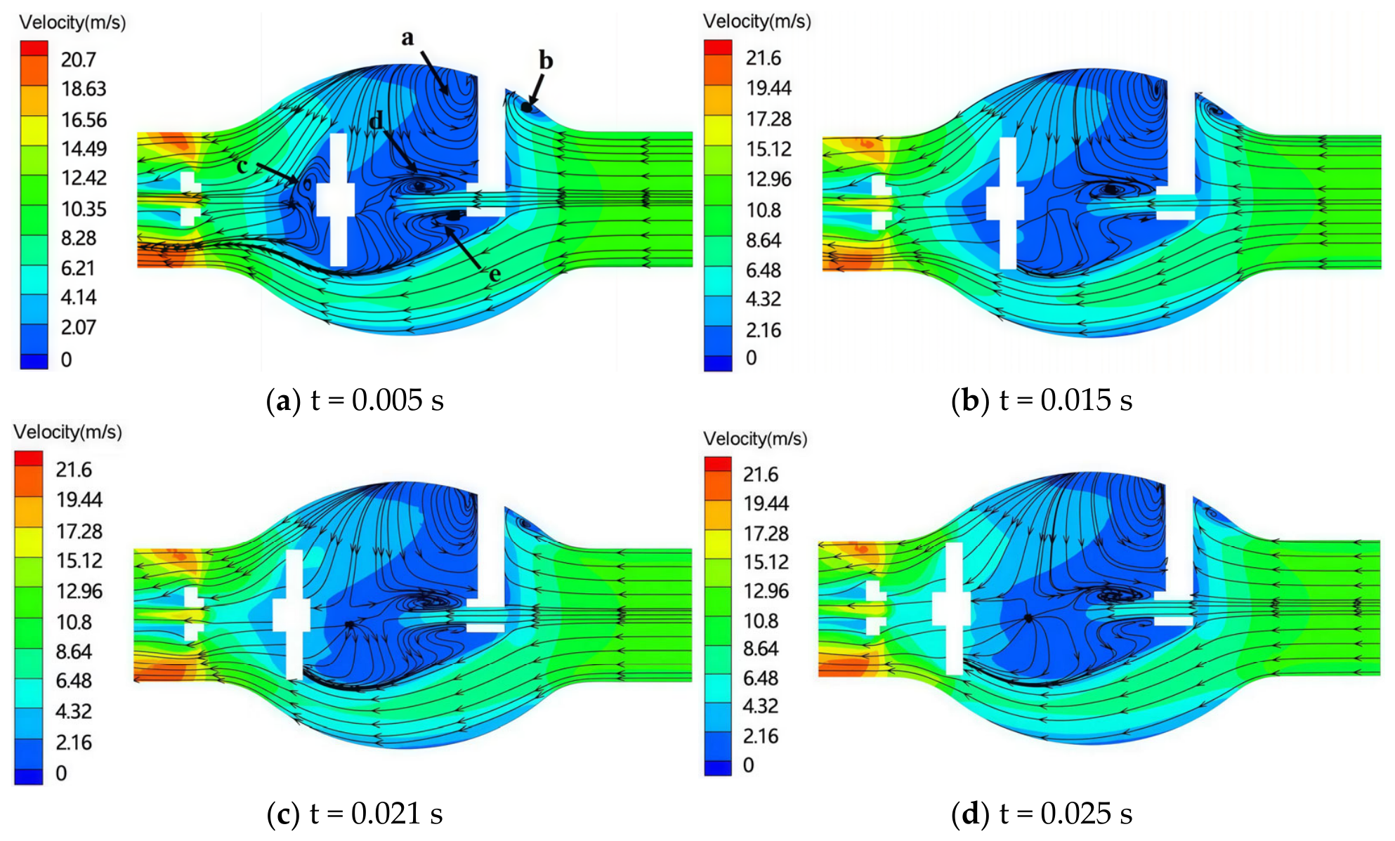
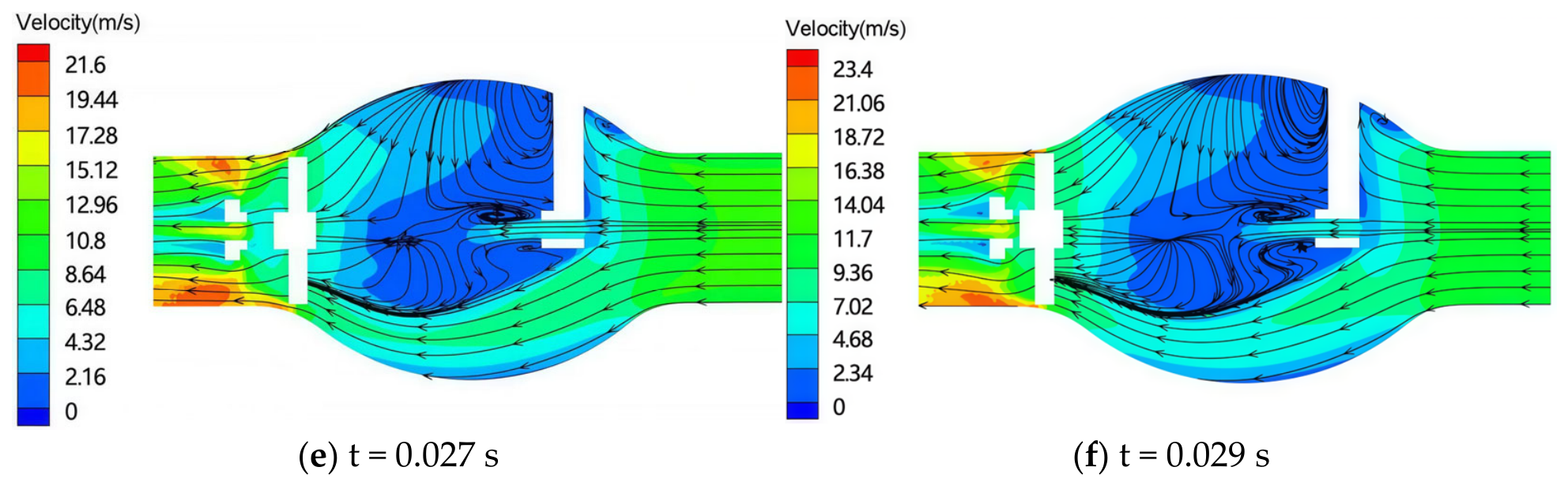
Figure 12 presents the velocity contours during valve closure. At t = 0.005 s, as closing begins, the velocity distribution at the outlet is relatively uniform. When the medium enters the chamber, its velocity decreases and continues to decrease as the distance to the wall becomes smaller, reaching approximately 2.1 m/s. High-velocity regions appear on the left side of the disk, with a maximum velocity of 20.5 m/s. Multiple small vortices form at positions a, b, c, d, and e in the chamber. Figure 12b–d shows the velocity distribution from t = 0.015 s to 0.025 s. As reverse flow develops, the pressure difference drives the disk leftward. The reverse-flow velocity increases, while the high-velocity region remains concentrated near the left side of the disk. Vortex c disappears, although other vortices remain, and the flow in these regions stays at low velocity. Figure 12e,f shows the velocity contours at t = 0.027 s and t = 0.029 s. At this stage, the valve is nearly closed. The small opening creates a jetting effect, producing a sharp increase in velocity at the throttling region. At t = 0.029 s, the maximum velocity in this region reaches 23.1 m/s. Once the valve fully closes, the reverse-flow path is completely blocked.

3.3.3. Valve-Disc Motion Characteristics During the Closing Process

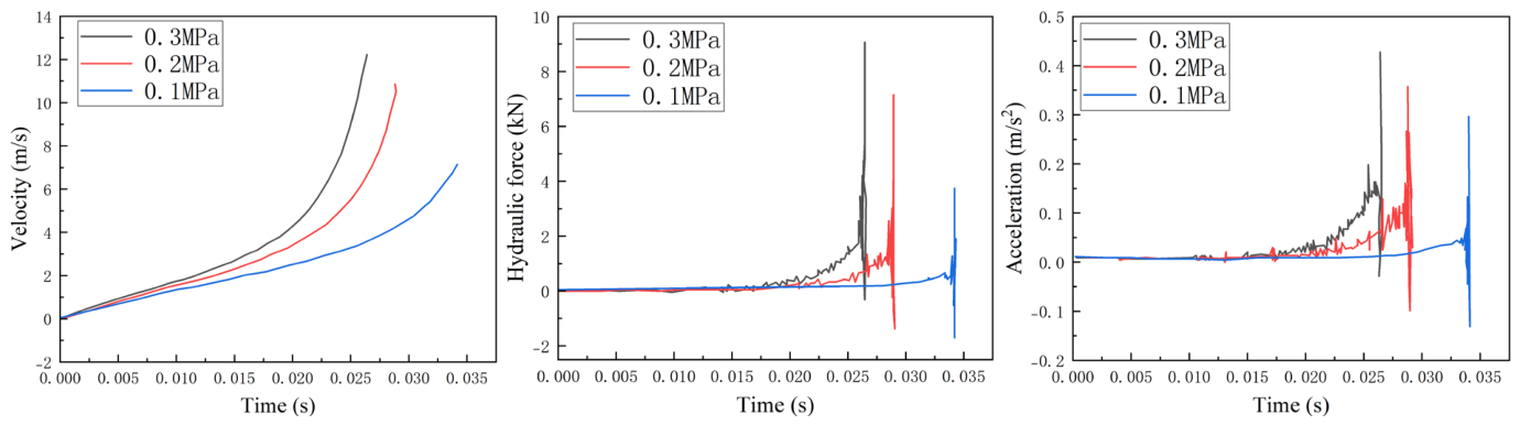
This section examines the dynamic behavior of the disk during valve closure under pressure differences of 100 kPa, 200 kPa, and 300 kPa. As shown in Figure 13, the velocity, acceleration, and hydrodynamic force acting on the disk increase with time. At the early stage of closure, the pressure difference across the disk is small, resulting in a nearly linear change in velocity with a low slope. As the opening continues to decrease, the pressure difference increases, causing the velocity curve to transition into a parabolic form and rise rapidly. Under a 300 kPa pressure difference, the maximum disk velocity reaches 12.9 m/s at the moment of closure. This occurs because, as the valve approaches full closure, the slopes of the acceleration and hydrodynamic-force curves increase, producing a parabolic rise. Near the end of closure, medium pressure becomes unstable. The disk undergoes oscillatory, variable-acceleration motion, which significantly increases the amplitude of acceleration and force fluctuations.

3.4. Disassembly and Failure Analysis of the Axial Flow Check Valve

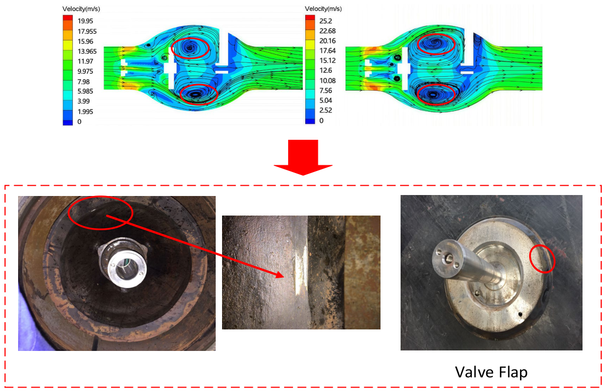
Figure 14 shows the disassembled axial-flow check valve used at the compressor-outlet pipeline of a compressor station in western China. During a start-up test on 14 September 2024, the valve operated normally; however, during shutdown, the disk failed to reseat in time, causing the compressor to rotate in reverse. Inspection of the failed valve revealed clear wear marks on both the support seat and the disk. The velocity contours show vortex formation within the valve chamber, while the transient simulations show hydrodynamic force fluctuations and oscillatory disk motion. Considered together, the numerical results and disassembly observations suggest a possible relationship between the unsteady flow, component wear, and delayed reseating. This interpretation is limited to the valve geometry and operating conditions described in Section 2.1 and Section 2.2.5. Similar valve geometries may also generate vortices near the valve seat; however, changes in valve diameter, pressure, flow rate, or gas composition can alter the vortex characteristics and disk motion. Therefore, the same wear and delayed-reseating behavior should not be assumed under other conditions.

4. Conclusions and Recommendations

Based on steady-state flow-field simulations and failure analysis of the axial flow check valve, the following conclusions and recommendations are proposed:

(1) When the medium enters the throttling region between the valve seat and the disk, the abrupt change in flow-passage cross-sectional area produces a significant velocity change. This sharp variation generates a distinct vortex region, reflecting energy loss as the fluid passes through the constricted area. The presence of the vortex increases turbulence intensity and may induce local pressure fluctuations that affect overall valve performance.

(2) During transient valve opening, a sudden pressure drop occurs as the fluid passes the disk. Flow disturbance near the disk leads to vortex formation inside the valve chamber. As the opening increases, the number of vortices also grows. Pressure fluctuations during opening cause the disk to oscillate, producing transient fluctuations in hydrodynamic force. These fluctuations, considered together with the disassembly observations, suggest a possible relationship between unsteady disk motion, the observed wear, and delayed reseating.

(3) During transient valve closure, the pressure decreases progressively after the fluid passes the disk. At the early stage of closure, multiple small vortices appear in the chamber center and near the pipe wall. As the opening decreases, the number of vortices gradually reduces until disappearing completely, whereas fluid velocity increases.

(4) Based on the abrupt changes in flow area, vortex formation, and observed component wear, potential design improvements include refining the valve-seat geometry and smoothing its transition to the adjacent flow passage, improving the stem and guide support, and considering wear-resistant materials or surface treatments for the guide sleeve and disk contact surfaces.

(5) To reduce failure risks under operating conditions, multiple operating scenarios should be evaluated, and the technical specifications for check valve procurement should be optimized to ensure suitability for the intended service conditions. Routine inspections should also be conducted to identify wear and potential reseating problems.

References

1. Feng, M. Transient Dynamic Analysis of Axial-Flow Check Valve Closure. Master’s Thesis, Lanzhou University of Technology, Lanzhou, China, 2016. [Google Scholar]
2. Zhang, Y.B.; Wang, H.B.; Zhang, X.Y. Design and experimental study of axial-flow control valve. Control Instrum. Chem. Ind. 2021, 48, 550–553, 588. [Google Scholar] [CrossRef]
3. Sotoodeh, K. Analysis and failure prevention of nozzle check valves used for protection of rotating equipment due to wear and tear in the oil and gas industry. J. Fail. Anal. Prev. 2021, 21, 1231–1239. [Google Scholar] [CrossRef]
4. Zhou, Q.Q.; Wang, Q.L.; Wang, X.; Tian, F. Study on the water hammer effect analysis and verification of nozzle check valve with damper for nuclear power plant. Fluid Meas. Control 2022, 3, 15–18. [Google Scholar]
5. Zhang, Q.L.; Huang, B.Y.; Yang, Z.D.; Yan, Y.; Li, G.D.; Guo, L.H. Water hammer properties of gas-bearing water pipeline using characteristics method. Trans. Chin. Soc. Agric. Eng. 2022, 38, 79–86. [Google Scholar] [CrossRef]
6. Tran, P.D. Pressure transients caused by tilting-disk check-valve closure. J. Hydraul. Eng. 2015, 141, 04014081. [Google Scholar] [CrossRef]
7. Zhang, G.; Guan, J.C.; Hu, R.H.; Tao, J.Y.; Chen, D.S.; Lin, Z. Numerical analysis of collision impact and sound noise in axial flow check valve. Eur. J. Mech. B Fluids 2025, 114, 204323. [Google Scholar] [CrossRef]
8. Makaryants, G.M. Fatigue failure mechanisms of a pressure relief valve. J. Loss Prev. Process Ind. 2017, 48, 1–13. [Google Scholar] [CrossRef]
9. Baran, G.; Catana, I.; Magheti, I.; Safta, C.A.; Savu, M. Controlling the cavitation phenomenon of evolution on a butterfly valve. IOP Conf. Ser. Earth Environ. Sci. 2010, 12, 012100. [Google Scholar] [CrossRef]
10. Zhang, W.T. Transient Pressure Distribution and Impact Analysis of an Axial-Flow Check-Valve Disc. Master’s Thesis, Lanzhou University of Technology, Lanzhou, China, 2014. [Google Scholar]
11. Wang, T. Dynamics of the Closing Process of an Axial-Flow Check Valve. Master’s Thesis, Lanzhou University of Technology, Lanzhou, China, 2017. [Google Scholar]
12. Beker, B.A.; Kansal, M.L. Pipe and isolation valve failure-impact analysis and prioritization model for an urban water distribution network. J. Hydroinform. 2023, 25, 491–510. [Google Scholar] [CrossRef]
13. Duan, F.B.; Min, X.H.; Wang, K.X.; Li, K. Process simulation for the opening of axial flow check valves based on fluid-solid coupling. Oil Gas Storage Transp. 2016, 35, 964–969. [Google Scholar]
14. Wu, X.K.; Gu, J.L.; Zhou, C.; Zhu, L.X.; Yu, G.; Tian, X.S. Research on opening and closing states of an axial-flow check valve at different flow rates. Valve 2024, 577–580, 597, No.5. [Google Scholar]
15. Botros, K.K. Spring stiffness selection criteria for nozzle check valves employed in compressor stations. J. Eng. Gas Turbines Power 2011, 133, 122401. [Google Scholar] [CrossRef]
16. Wang, S.L.; Zhang, Y.; Bai, N.Y.; Cai, Y.M. The failure finite element analysis of pump collision with valve in the oil well pump. Adv. Mater. Res. 2013, 690–693, 3112–3115. [Google Scholar] [CrossRef]
17. Sun, B.Y. Stability of a Check-Valve Core Considering Fluid–Structure Interaction. Master’s Thesis, Lanzhou University of Technology, Lanzhou, China, 2022. [Google Scholar]
18. Nilsson, J.O.; Nilsson, L.; Oldenburg, M. Impact stresses in flapper valves: A finite element analysis. In Proceedings of the 1980 International Compressor Engineering Conference, West Lafayette, IN, USA, 23–25 July 1980. [Google Scholar]
19. Himr, D.; Habán, V.; Hudec, M. Experimental investigation of check valve behaviour during the pump trip. J. Phys. Conf. Ser. 2017, 813, 012054. [Google Scholar] [CrossRef]
20. Himr, D.; Habán, V.; Dokoupil, P. Check valve slam analysis in pumping station. EPJ Web Conf. 2016, 114, 02038. [Google Scholar] [CrossRef]
21. Li, S.X.; Hou, Y.Z.; Li, L.C. Dynamic characteristics of swing check valve based on dynamic mesh and UDF. Appl. Mech. Mater. 2013, 321–324, 86–89. [Google Scholar] [CrossRef]
22. Zhang, X.H.; Feng, M.; Zhang, Y.B. Transient analysis of the closing process of an axial-flow check valve. Machinery 2016, 54, 51–53. [Google Scholar] [CrossRef]
23. Zhang, N.; Zhang, X.H.; Wang, T.; Wang, Y. Simulation analysis of the closing process of the disc of an axial-flow check valve. Machinery 2019, 57, 44–47. [Google Scholar] [CrossRef]
24. Wang, T.; Zhang, Y.J.; Kong, B.B.; Wu, J.; Ni, X. Analysis of instantaneous collision process of axial flow check valve closing. J. Phys. Conf. Ser. 2021, 2005, 012176. [Google Scholar] [CrossRef]
25. Li, K.L.; Wang, H.M.; Wang, J.X.; Zhao, Y. Analysis of the internal flow field of low flow resistance coefficient axial flow type check valve. J. Eng. Therm. Energy Power 2017, 32, 78–83. [Google Scholar]
26. Song, X.G.; Cui, L.; Park, Y.C. Three-dimensional CFD analysis of a spring-loaded pressure safety valve from opening to re-closure. In Proceedings of the ASME 2010 Pressure Vessels and Piping Division/K-PVP Conference, Bellevue, WA, USA, 18–22 July 2010; Volume 5, pp. 295–303. [Google Scholar] [CrossRef]
27. Turesson, M. Dynamic Simulation of Check Valve Using CFD and Evaluation of Check Valve Model in RELAP5. Master’s Thesis, Chalmers University of Technology, Gothenburg, Sweden, 2011. [Google Scholar]
28. Dallstream, B.E.; Fricke, B.A.; Becker, B.R. Swing check valve design criteria and CFD validation. In Proceedings of the 14th International Conference on Nuclear Engineering (ICONE14), Miami, FL, USA, 17–20 July 2006; Volume 1, pp. 691–699. [Google Scholar] [CrossRef]
29. Guan, A.Q.; Xu, J.X.; Jin, Z.J.; Qian, J.Y. Damping effect and fluid dynamic analysis on closing process of axial flow check valve. J. Fluids Eng. 2023, 145, 101204. [Google Scholar] [CrossRef]
30. Lin, Z.H.; Hou, C.W.; Zhang, L.; Guan, A.Q.; Jin, Z.J.; Qian, J.Y. Fluid-structure interaction analysis on vibration characteristics of sleeve control valve. Ann. Nucl. Energy 2023, 181, 109579. [Google Scholar] [CrossRef]
31. Zhao, L.; Chang, Z.B.; Mai, C.L.; Ran, H.; Jiang, J. Experimental and numerical investigation on dynamic characteristic of nozzle check valve and fluid-valve transient interaction. Nucl. Eng. Des. 2024, 416, 112737. [Google Scholar] [CrossRef]
32. Wang, F.; Zeng, Y.S.; Wang, W.; Chen, F.; Gao, W.; Yan, H.; Li, J. Transient flow characteristics for fluid-structure interaction on hydrogen decompression valve in high-pressure hydrogen storage systems. Int. J. Hydrogen Energy 2024, 79, 1250–1266. [Google Scholar] [CrossRef]
33. Qu, S.G.; Li, D.A.; Li, J.H.; Sun, P.; Li, X.; Sun, G. Investigate the impact wear failure behavior of CoMoCr engine valve and valve seat pairs under harsh conditions. Eng. Fail. Anal. 2025, 167, 109052. [Google Scholar] [CrossRef]
34. Wang, Q.L.; Wang, X.S.; Tian, F. Study on the closing dynamic characteristics of nuclear power axial flow check valve. Valve 2024, 1142–1149, No.9. [Google Scholar]
Figure 1. Structure and principal components of the axial flow check valve.
Processes 14 02407 g001
Figure 2. Force diagram of the valve disk.
Processes 14 02407 g002
Figure 3. Three-dimensional flow-passage model of the axial-flow check valve.
Processes 14 02407 g003
Figure 4. Mesh model of the axial-flow check valve.
Processes 14 02407 g004
Figure 5. Smoothing and local remeshing settings used for the dynamic-mesh calculations.
Processes 14 02407 g005
Figure 6. Comparison of CFD-predicted and experimentally measured pressure drops for the fully open valve.
Processes 14 02407 g006
Figure 7. Steady-state pressure and velocity contours at 100% valve opening.
Processes 14 02407 g007
Figure 8. Transient pressure contours at selected times during valve opening.
Processes 14 02407 g008
Figure 9. Transient velocity contours at selected times during valve opening.
Processes 14 02407 g009
Figure 10. Steady-state and transient hydrodynamic forces on the disk.
Processes 14 02407 g010
Figure 11. Transient pressure contours at selected times during valve closure.
Processes 14 02407 g011aProcesses 14 02407 g011b
Figure 12. Transient velocity contours at selected times during valve closure.
Processes 14 02407 g012aProcesses 14 02407 g012b
Figure 13. Disk motion and hydrodynamic force during valve closure under different pressure differences.
Processes 14 02407 g013
Figure 14. Localized wear observed on the support seat and disk of the failed axial-flow check valve.
Processes 14 02407 g014