Analysis of Key Factors Controlling Fractured Wells Productivity in Tight Gas Condensate Reservoirs Based on Machine Learning Surrogate Models and SHAP

Abstract

To address the complex factors affecting the productivity of fractured horizontal wells in tight condensate gas reservoirs, as well as the high computational costs and opaque mechanism interpretation associated with traditional numerical simulations, this study proposes and implements a quantitative evaluation method for the main productivity-controlling factors. This method integrates a machine learning surrogate model with the Shapley additive explanations (SHAP) interpretability framework. First, based on 3D geological modeling and fracture propagation simulation, a high-dimensional parameter set encompassing reservoir geology, artificial fractures, and fluid properties was constructed. Subsequently, representative samples were generated through an orthogonal experimental design. On this basis, machine learning algorithms, including Support Vector Machines (SVM), Random Forests (RF), and eXtreme Gradient Boosting (XGBoost), were utilized to construct low-cost, high-precision surrogate models targeting initial productivity and Estimated Ultimate Recovery (EUR). These surrogate models effectively substituted the computationally expensive fully coupled numerical simulations. Furthermore, SHAP values were applied to the trained surrogate models to conduct both global and local interpretability analyses. This approach not only quantifies the magnitude and direction of each input parameter’s contribution to the productivity predictions, but also reveals their non-linear mechanisms and interaction effects. The results indicate that reservoir properties and gas saturation are the fundamental factors determining the productivity of fractured horizontal wells, while fracture conductivity and fracture half-length are the key engineering factors. Furthermore, there exist significant synergistic or antagonistic effects between the geological and engineering parameters. The integrated “parametric modeling–surrogate model construction—SHAP interpretability analysis” workflow established in this study provides a highly efficient, transparent, and physically insightful novel approach for the rapid optimization of fracturing designs and the mechanistic analysis of main productivity-controlling factors in tight condensate gas reservoirs.

1. Introduction

As a crucial unconventional hydrocarbon resource, tight condensate gas reservoirs rely heavily on horizontal drilling and large-scale hydraulic fracturing technologies for their efficient development [1,2]. However, practical field development faces complex “geology-engineering-fluid” coupling challenges: severe reservoir heterogeneity, retrograde condensate blockage in the near-wellbore region, and complex interactions between the hydraulic fracture network and the rock matrix collectively dictate the ultimate production performance [3,4]. Traditional productivity evaluation primarily relies on physics-based numerical simulations or statistics-based empirical methods [5]. While the former rigorously captures the underlying physical mechanisms, it is hindered by complex modeling procedures and prohibitive computational costs, rendering it impractical for large-scale parameter sensitivity analysis and real-time optimization [6,7]. Conversely, the latter struggles to reveal the complex non-linear relationships and interaction effects among multiple factors, suffering from inadequate generalization capability and a lack of physical interpretability [8,9]. Consequently, both approaches exhibit a pronounced trade-off between computational efficiency and mechanistic depth.

Determining the main productivity-controlling factors for fractured horizontal wells is highly challenging, a difficulty fundamentally rooted in the fact that subsurface reservoirs are inherently highly heterogeneous systems [10]. Spatial variability is omnipresent, spanning from macroscopic structures and sedimentary facies to microscopic pore structures and from rock mineral compositions to the distribution of in situ stress fields. It is precisely within such a heterogeneous geomechanical environment that hydraulic fractures initiate, propagate, and intersect. Consequently, the ultimate fracture geometry and conductivity are not solely dictated by surface operational parameters. Instead, they emerge from the dynamic coupling and joint interactions between multiple geological factors—including subsurface rock mechanical properties, in situ stress states, and natural fracture systems—and surface engineering inputs. Neglecting this coupling and designing fracturing treatments based purely on empirical or statistical rules often results in insufficient fracture propagation, ineffective propping, or even unintended communication with detrimental water zones, thereby incurring a massive waste of both resources and capital.

To address the aforementioned challenges, the prevailing solution in both industry and academia is to construct an integrated geology-engineering numerical simulation workflow [11,12]. This workflow begins with high-fidelity 3D geological modeling. Utilizing mainstream platforms such as Petrel, this step integrates seismic interpretations, well log data, and geological insights to construct a 3D geological model capable of reflecting the structural framework and the spatial distribution of reservoir properties. Building further upon this, based on sonic and density well logs, mechanical parameters are populated into the 3D grid cells through rock physics modeling, thereby establishing a comprehensive geomechanical parameter model. This static model constitutes the closest mathematical representation of the actual subsurface conditions. Subsequently, this model is imported into specialized hydraulic fracturing simulation software. Under precise mechanical boundary conditions, the dynamic propagation of fractures within heterogeneous stress fields and lithologies is simulated [13]. This effectively bridges the static geological characterization with the dynamic fracturing response, accomplishing the crucial transition from a geological model to a fracture model. However, obtaining the fracture model is not the endpoint of the research, but rather a new starting point for rigorous quantitative analysis. The fracture simulation yields a vast array of fracture properties, which, together with the original geological and engineering parameters, constitute a high-dimensional parameter space that potentially governs the ultimate production performance. Identifying these critical governing factors and elucidating their impact on productivity from such complex data is the cornerstone of optimizing stimulation design and achieving “sweet-spot” targeted fracturing [14]. Conventional single-factor analyses or empirical engineering judgments frequently break down within such a complex system. Consequently, it is imperative to employ more rigorous and robust statistical methods to isolate the genuinely dominant factors within this multivariate system and reveal their underlying mechanisms.

In recent years, machine learning (ML) techniques have emerged as a novel pathway to break through this bottleneck [15,16]. By training surrogate models, high-fidelity and computationally efficient mathematical mappings can be established between high-dimensional input parameters and target outputs [17]. These models can thereby replace time-consuming numerical simulators, enabling rapid productivity forecasting and the exhaustive screening of massive design scenarios. However, complex machine learning models, typified by deep learning, are often regarded as “black boxes” whose internal decision-making logic is difficult to interpret. This lack of transparency severely hinders engineers’ trust in the model predictions and makes it difficult to extract patterns with clear physical or engineering significance [18]. Consequently, in oil and gas reservoir development—a domain that demands exceptionally high reliability in decision-making—model interpretability is equally as important as predictive accuracy. This constitutes the “second dilemma” that must be resolved to successfully apply advanced machine learning methods. Fortunately, the advancement of Explainable Artificial Intelligence provides the necessary toolkit to address these challenges. Among these, the SHAP method, based on cooperative game theory, provides a unified and robust framework to quantify the contribution of each feature to an individual prediction across any complex model [19]. It not only addresses the global question of which factor is the most significant but also elucidates how various factors interact to drive the prediction outcome for any specific sample [20]. Integrating SHAP with machine learning surrogate models holds the potential to ‘open the black box’ while preserving high computational efficiency, thereby translating data-driven conclusions into interpretable and verifiable engineering insights [21].

In light of this background, this study focuses on a core engineering issue: analyzing the main controlling factors of productivity for hydraulically fractured horizontal wells in tight gas condensate reservoirs. We aim to establish and demonstrate an integrated workflow that couples machine learning surrogate models with SHAP-based interpretability analysis. Specifically, this study will first utilize high-fidelity numerical simulation to generate a training sample database and subsequently deploy advanced machine learning algorithms, such as Gaussian process regression, to construct a high-accuracy proxy model for productivity prediction [22]. Subsequently, the SHAP method is systematically applied to conduct an in-depth analysis of the surrogate model from multiple dimensions, including global feature importance, the direction of feature effects, and feature interaction effects [23]. The ultimate objective is not merely to establish an efficient predictive tool but further to quantitatively and intuitively elucidate the complex interaction mechanisms and importance rankings among key geological parameters, fracture properties, and production regimes governing well productivity. This aims to provide data-driven intelligent support—characterized by efficiency, accuracy, and transparency—for optimizing fracture designs and formulating field development strategies [24]. This study aspires to provide an exemplary methodology to advance the application of machine learning in oil and gas reservoir development, propelling the transition from ‘black-box’ predictions to ‘white-box’ decision support [25].

2. Geological Setting

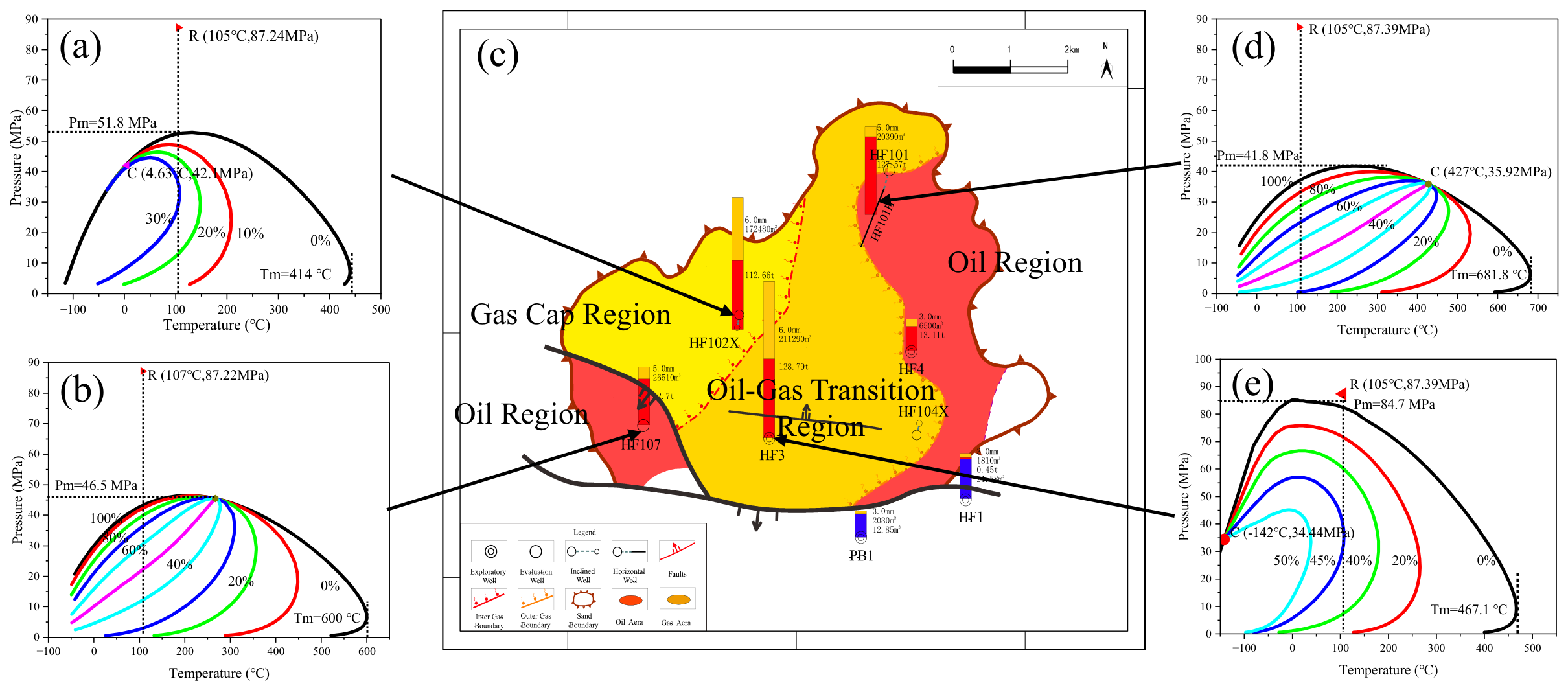
The study area, block HF3, is located in the Central Depression of the Junggar Basin. As one of the primary hydrocarbon-rich sags in the basin, it extends generally in a northeast direction. In ascending order, the Baijiantan Formation in block HF3 is subdivided into three members: T₃b₁, T₃b₂, and T₃b₃. The T₃b₂ member is further subdivided into three sand sets, with the first sand set, T₃b₂¹, primarily composed of fine sandstone and argillaceous siltstone, the second sand set, T₃b₂², is dominated by mudstone and silty mudstone, while the third sand set, T₃b₂³, is characterized by unequal interbeds of fine sandstone, mudstone, and silty mudstone. Notably, hydrocarbon shows are observed across all three sand sets. At present, oil and gas exploration successes within the Baijiantan Formation in the study area are primarily concentrated in T₃b₂¹. Here, the sand bodies exhibit stable lateral distribution, substantial reservoir thickness, and favorable petrophysical properties, accompanied by widespread hydrocarbon shows. The T₃b₂¹ interval features an initial reservoir pressure of 87.5 MPa, a pressure coefficient of 1.97, and a formation temperature of 105 °C, classifying it as a high-pressure hydrocarbon reservoir. Based on the PVT fluid phase behavior simulations conducted on four representative wells (HF102X, HF3, HF107, and HF101H), block HF3 was subdivided into four distinct regions, as depicted in Figure 1. At the structural crest of the reservoir, the HF102X well area is identified as a gas condensate reservoir, while the HF3 well area acts as a gas-oil transition zone. Moving downdip, the HF107 well area and the basal HF101H well area are characterized as black oil reservoirs approaching volatile oil behavior. During the reservoir exploration and appraisal phase, various well types were trialed for development; however, a significant discrepancy in productivity was observed among different well configurations. Furthermore, the extremely complex distribution of reservoir fluids across different zones, combined with poorly defined primary controls on well performance, has hindered development progress. Consequently, there is an urgent need to clarify the main controlling factors affecting well productivity in block HF3.

3. Integrated Geology-Engineering Productivity Evaluation Model

3.1. Hydraulic Fracture Modeling for Tight Gas Reservoirs

3.1.1. 3D Geological Modeling

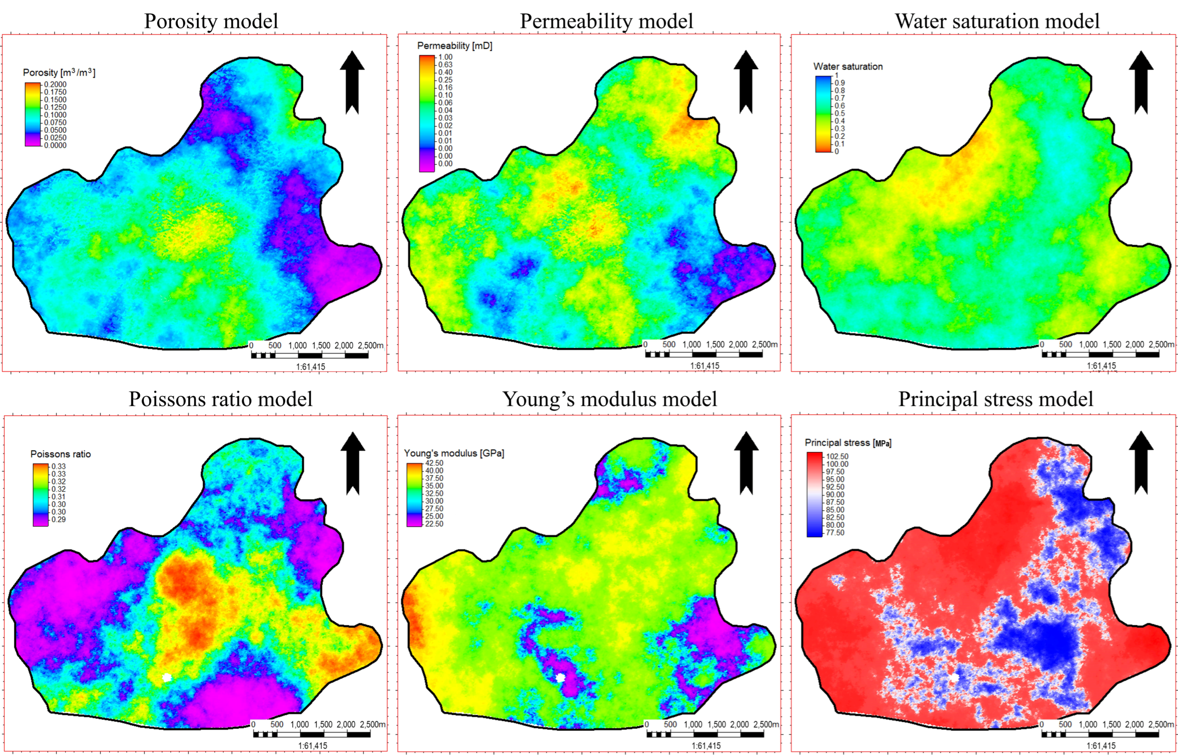
Based on seismically interpreted horizons, faults, and well data, a structural model is constructed via framework modeling to define the 3D spatial framework of the formation. Subsequently, within the structural grid, log-derived porosity and permeability are utilized as hard data to construct petrophysical property models. This is achieved by incorporating stochastic modeling methods, such as variogram analysis and Sequential Gaussian Simulation. Based on sonic, density, and other well logs, well-point data for parameters such as Young’s modulus and Poisson’s ratio are derived using empirical correlations or rock physics models. These parameters are subsequently treated as new properties and distributed throughout the 3D structural grid via spatial interpolation or stochastic simulation, generating continuous 3D geomechanical property volumes. The modeling of the maximum and minimum horizontal principal stresses is typically based on the pore pressure model, the overburden pressure model, and tectonic stress coefficients. These stresses are computed and populated in 3D space using mechanical equations, thereby yielding a static model coupled with the geological model that is suitable for geomechanical analysis [26]. Figure 2 illustrates the geological and geomechanical property models of the target area.

3.1.2. Hydraulic Fracture Simulation

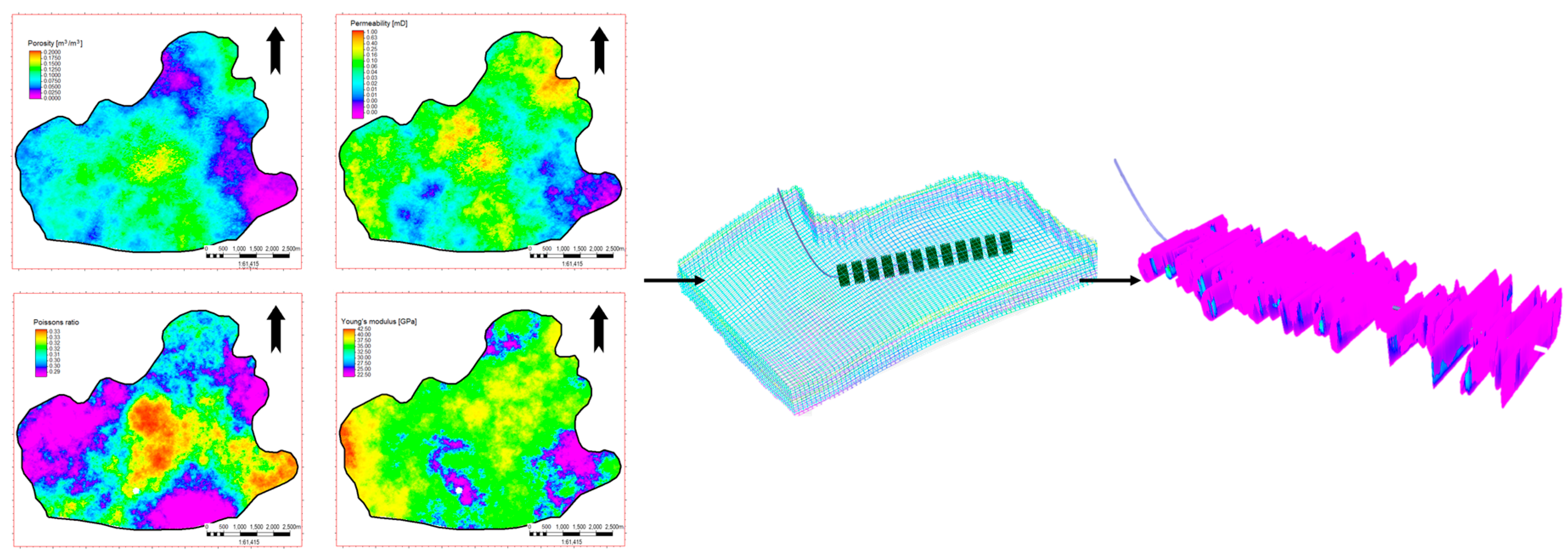
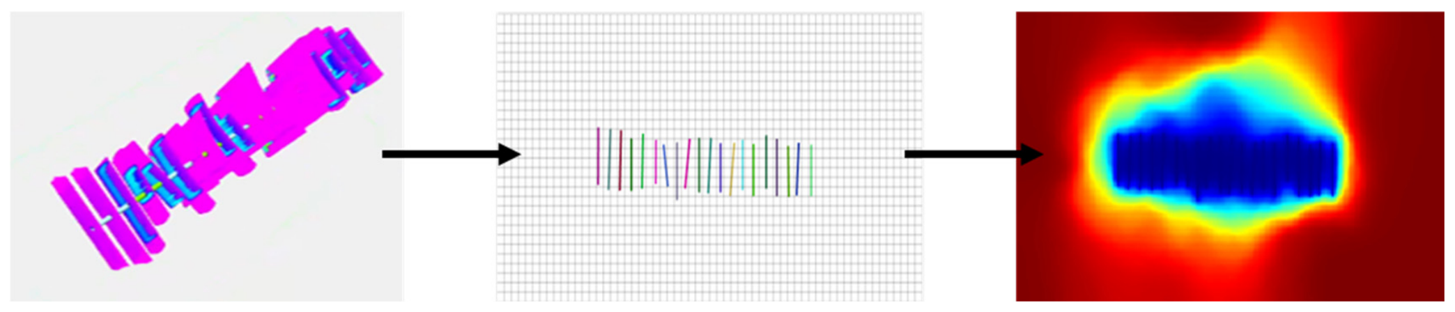
Based on high-resolution 3D geological and geomechanical property models, conducting numerical simulation of hydraulic fractures for fractured horizontal wells in tight gas reservoirs is a critical step in optimizing fracture design and evaluating development performance. The geometry and spatial propagation of the fractures are directly governed by the reservoir geomechanical parameters captured within the models, such as the heterogeneous in situ stress field and the rock brittleness index. The process of acquiring hydraulic fracture geometries follows these core steps: First, the static geological model—incorporating the structural framework, heterogeneous reservoir properties, and 3D spatial distribution of geomechanical parameters—is imported into Kinetix, a geomechanics-coupled hydraulic fracturing simulator. Secondly, the horizontal wellbore trajectory, perforation cluster locations, and fracturing treatment parameters are defined within the simulator. Based on continuum mechanics theory, fracture initiation and propagation are simulated by solving the coupled equations of fluid flow and rock deformation. The overall workflow is illustrated in Figure 3. Through these steps, the hydraulic fracture model for the fractured horizontal well is established. Subsequently, the simulated 3D fracture geometries and conductivity distributions are imported into a gas reservoir simulation model as key input parameters to conduct production forecasting. To generate the training dataset, hydraulic fracture propagation was simulated using the Kinetix (Version 2022.2) reservoir-centric stimulation-to-production software. The simulations were performed using the Unconventional Fracture Model (UFM), a fully coupled numerical solution that explicitly accounts for reservoir heterogeneity, stress anisotropy, and complex fracture interactions, including multi-level stress-shadow effects in both 2D and 3D. The UFM solves for fracture propagation mechanics coupled with proppant transport, enabling realistic prediction of complex fracture networks [27]. Key model assumptions and input parameters were defined based on the geologic and geomechanical characterization of the target reservoir. The specific simulation process is consistent with the study by [28].

3.2. Productivity Prediction Model for Fractured Horizontal Wells in Tight Gas Condensate Reservoirs

The Embedded Discrete Fracture Model (EDFM) is utilized to embed the hydraulic fracture network into the reservoir matrix grids, thereby establishing a coupled matrix-fracture flow model. To account for the characteristics of the gas condensate reservoir, a compositional model is employed to accurately capture the fluid phase behavior [29].

3.2.1. Mathematical Model

The mass conservation equation for each hydrocarbon component in the oil and gas phases is expressed as follows:

$$\nabla \cdot \left({\rho }_l{X}_l^i{\overrightarrow{v}}_l+{\rho }_v{X}_v^i{\overrightarrow{v}}_v\right)+{\partial }_t\left[\varphi \left({\rho }_l{S}_l{X}_l^i+{\rho }_v{S}_v{X}_v^i\right)\right]=\left({\rho }_l{X}_l^i{q}_l+{\rho }_v{X}_v^i{q}_v\right)/V$$

(1)

If a water phase is present, its mass conservation equation can be written as follows:

$$\nabla \cdot \left({\rho }_w{\overrightarrow{v}}_w\right)+{\partial }_t\left(\varphi {\rho }_w{S}_w\right)={\rho }_w{q}_w/V$$

(2)

In the conservation equations, $\varphi$ represents the porosity; ${\rho }_{\alpha }$ and $S_{\alpha }$ denote the mass density and saturation of phase $\alpha$, respectively; and $X_l^i$ and $X_v^i$ represent the mass fractions of each component I in the liquid and vapor phases, respectively.

${\overrightarrow{v}}_w$, ${\overrightarrow{v}}_l$, and ${\overrightarrow{v}}_v$ represent the velocity vectors of the water, liquid, and vapor phases in the matrix, respectively. Considering the threshold pressure gradient and stress sensitivity in tight sandstone gas reservoirs, the governing flow equation is expressed as:

$${\overrightarrow{v}}_{\alpha }=-\mathit{K}{\displaystyle \frac{k_{\alpha }(s)}{{\mu }_{\alpha }}}\left(\nabla p_{\alpha }-{\rho }_{\alpha }g\nabla z\right)=-\mathit{K}{\lambda }_{\alpha }\left(\nabla p_{\alpha }-{\rho }_{\alpha }g\nabla z\right)$$

(3)

where $\mathit{K}$ is the permeability of the medium, ${\mathrm{m}}^{-2}$; $k_{r\alpha }$ is the relative permeability of phase $\alpha$; ${\mu }_{\alpha }$ is the viscosity of fluid phase $\alpha$, $\mathrm{m}\mathrm{P}\mathrm{a}·\mathrm{s}$; $\nabla p$ is the pressure gradient, Pa/m; $p_0$ is the initial reservoir pressure, $\mathrm{P}\mathrm{a}$; and $\lambda$ is the threshold pressure gradient, Pa/m. Additionally, $\lambda$ denotes the permeability modulus of the porous medium, $\mathrm{P}{\mathrm{a}}^{-1}$, which varies between the matrix and fractures.

When accounting for the threshold pressure gradient and stress sensitivity, and incorporating relevant experimental data, the fluid flow equation is expressed as:

$${\overrightarrow{v}}_{\alpha }=-K{\lambda }_{\alpha }{e}^{-\beta \nabla p}\left(\nabla p_{\alpha }-{\rho }_{\alpha }g\nabla z-{\lambda }_B\right)$$

(4)

The saturation and compositional constraints also apply to the governing equations:

$$S_w+S_v+S_l=1$$

(5)

$$\left\{\begin{array}{l}{\displaystyle {\sum }_{i=1}^N{X}_l^i}=1\\ {\displaystyle {\sum }_{i=1}^N{X}_v^i}=1\end{array}\right.$$

(6)

The viscosities and relative permeabilities of the oil and vapor phases are determined via laboratory measurements. The densities and mole fractions of the oil and vapor phases are calculated using the modified Peng–Robinson Equation of State (PR-EOS):

$$p={\displaystyle \frac{RT}{V-b_m}}-{\displaystyle \frac{a_m\left(T\right)}{V\left(V+m_1{b}_m\right)+b_m\left(V+m_2{b}_m\right)}}$$

(7)

where am and bm are the average attraction and repulsion constants of the mixture, respectively.

3.2.2. Embedded Discrete Fracture Model (EDFM)

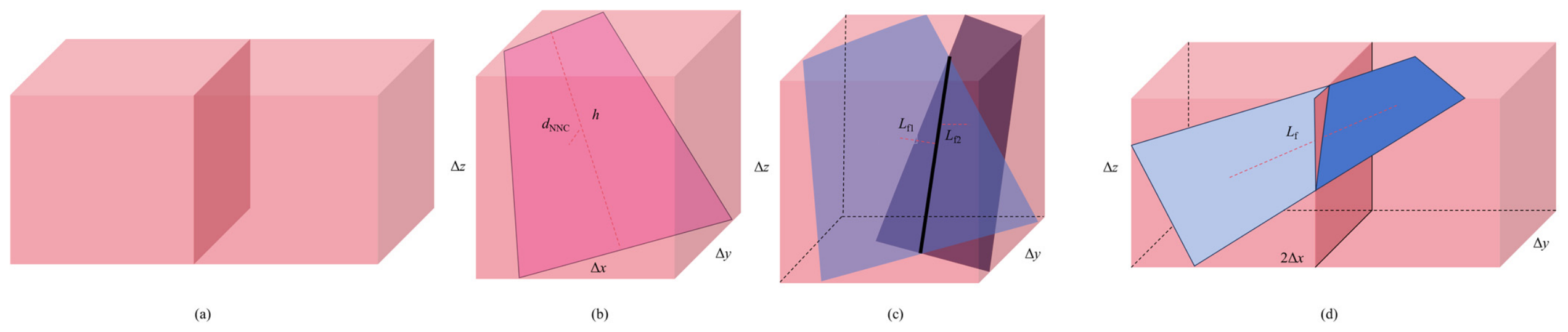
The EDFM is an advanced numerical approach highly efficient in handling flow simulations within complex fracture networks. By directly embedding discretized fracture elements into the structured matrix grid, it employs Non-Neighbor Connections (NNC) to accurately compute fluid exchange between the fractures and the matrix. This approach circumvents the grid-generation complexity associated with local grid refinement (LGR) along fracture faces inherent in conventional methods [30]. While maintaining high computational efficiency, it precisely characterizes the non-Darcy flow and mass transfer processes within fractures of arbitrary geometries and orientations, serving as a critical technology for the high-fidelity production simulation and forecasting of fractured horizontal wells. Therefore, this study utilizes the EDFM to simulate fractured horizontal wells, where the calculation of transmissibility serves as the cornerstone for the model to accurately capture the fluid exchange among the fracture, matrix, and wellbore systems. These transmissibilities are categorized into three primary types and computed based on rigorous geometric and flow principles: matrix-matrix transmissibility (Figure 4a), fracture-matrix transmissibility (Figure 4b), and fracture-fracture transmissibility (Figure 4c,d).

The matrix-matrix transmissibility ($T_{pMM}$) is calculated using the following formula:

$$T_{pMM}=K{\displaystyle \frac{A-A_{\perp x}}{\Delta {\overrightarrow{x}}_e}}$$

(8)

In Equation (8), $\mathsf{\Delta }{\overrightarrow{x}}_e$ represents the grid block sizes in all three spatial directions; A denotes the area between the projection plane and the matrix grid; and $A_{\perp x}$ signifies the projected area. When the internal fracture element completely intersects the host matrix grid block and runs parallel to the interface between the projection plane and the host matrix grid, the projected area reaches its maximum value, equaling A. Conversely, when the orientation of the internal fracture grid is perpendicular to the interface between the projection plane and the host matrix grid, it reduces to zero.

The matrix-fracture transmissibility is calculated using the following formula:

$$T_{pMF}={\displaystyle \frac{A_{\perp x}{K}_{pMF}}{d_{pMF}}}$$

(9)

Therein

$$K_{pMF}={\displaystyle \frac{K_{pM}{K}_f}{K_{pM}+K_f}}$$

(10)

Here, $\left(T_{pMF}\right)$ represents the harmonic mean of the permeabilities of the projected matrix and fracture grids, $\left(d_{pMF}\right)$ denotes the distance between the fracture centroid and the projected grid, and $A_{\perp x}$ is the projected area of the fracture along each dimension.

The transmissibility between different fractures is calculated using the following formula:

$$T_{pFF}={\displaystyle \frac{T_{F1}{T}_{F2}}{T_{F1}+T_{F2}}}$$

(11)

The calculation method for the transmissibility between different fracture grid cells within the same fracture is analogous to that between conventional matrix grid blocks.

3.3. Productivity Evaluation Model Coupling Geological and Engineering Factors

3.3.1. Evaluation Workflow

Upon obtaining the parameters of the complex fracture network via Kinetix hydraulic fracturing simulations, this study employs the EDFM to conduct numerical simulations of production performance for fractured horizontal wells. By directly embedding discretized fracture elements into structured matrix grids and establishing NNC, the EDFM approach efficiently captures the fluid exchange between the fractures and the matrix. In the simulation, the 3D fracture geometries and spatially variable conductivity output from Kinetix are parameterized and integrated into the reservoir numerical simulator, establishing a refined ‘matrix-fracture-wellbore’ coupled flow model. To account for the distinct characteristics of tight condensate gas reservoirs, a compositional model is adopted to accurately characterize the variations in fluid phase behavior. Numerical simulations are conducted to predict long-term production performance, quantitatively analyzing the controlling effects of fracture, reservoir, and fluid parameters on productivity; the comprehensive productivity evaluation workflow is illustrated in Figure 5. Transitioning from Kinetix-based fracture propagation to the EDFM-based productivity evaluation model constructs a high-fidelity training dataset for this study, providing a reliable data foundation to subsequently perform an interpretable machine learning analysis on the primary controlling factors of well productivity.

Based on the established integrated geological-engineering production evaluation model, a production forecasting program incorporating geological, fluid, engineering, and development parameters was developed. The input and output parameters are shown in Table 1. Utilizing the Latin Hypercube Sampling (LHS) method, 400 parameter sets were generated to simulate the initial production and Estimated Ultimate Recovery (EUR) of a single well under various parameter combinations, thereby providing a robust data foundation for analyzing the primary controlling factors of productivity.

Table 1. Influencing factors and parameter ranges for fractured horizontal well productivity in the target area.

Type		Parameter	Range of Values/Remarks
Input Parameters	Geological Parameters	Porosity	0.08~0.12
		Permeability	0.1~1 mD
		Oil Saturation	0.45~0.6
		Pay Zone Thickness	6~15 m
	Fluid Parameters	Crude Oil Viscosity	4~10 mPa·s
		Residual Gas Saturation	0.25~0.35
		Irreducible Water Saturation	0.3~0.45
		Crude Oil Density	790~860 kg/m3
		Threshold Pressure Gradient	0.02~0.08 MPa/m
		Stress Sensitivity Coefficient	2 × 10−7~9 × 10−7  Pa−1
	Engineering Parameters	Injection Rate	8~12 m3/min
		Proppant Intensity	3~6 t/d
		Fluid Intensity	60~100 m3/m
	Development Parameters	Lateral Length	800~2000 m
		Fracture Half-Length	Based on simulation results
		Fracture Width
		Fracture Permeability
Output Parameters	/	Initial Productivity	/
		EUR	/

Table 1. Influencing factors and parameter ranges for fractured horizontal well productivity in the target area.

Type		Parameter	Range of Values/Remarks
Input Parameters	Geological Parameters	Porosity	0.08~0.12
		Permeability	0.1~1 mD
		Oil Saturation	0.45~0.6
		Pay Zone Thickness	6~15 m
	Fluid Parameters	Crude Oil Viscosity	4~10 mPa·s
		Residual Gas Saturation	0.25~0.35
		Irreducible Water Saturation	0.3~0.45
		Crude Oil Density	790~860 kg/m3
		Threshold Pressure Gradient	0.02~0.08 MPa/m
		Stress Sensitivity Coefficient	2 × 10−7~9 × 10−7  Pa−1
	Engineering Parameters	Injection Rate	8~12 m3/min
		Proppant Intensity	3~6 t/d
		Fluid Intensity	60~100 m3/m
	Development Parameters	Lateral Length	800~2000 m
		Fracture Half-Length	Based on simulation results
		Fracture Width
		Fracture Permeability
Output Parameters	/	Initial Productivity	/
		EUR	/

It is important to emphasize that the parameters related to near-wellbore damage and long-term fracture conductivity degradation were not treated as variables in the subsequent LHS design. Instead, they were fixed at the values calibrated through the history-matching procedure on well HF101H. By fixing these two parameters, we ensure that the LHS-generated dataset systematically captures the isolated and interactive effects of the primary geological, fluid, and engineering variables on well productivity. This methodological choice enhances the interpretability of subsequent SHAP analysis by eliminating confounding effects originating from localized, well-specific artifacts, thereby enabling a clearer attribution of productivity variations to the reservoir- and fracture-scale controlling factors.

3.3.2. Verification of the Productivity Evaluation Model

To ensure that the constructed integrated geological-engineering production evaluation model possesses reliable predictive capabilities, a systematic validation of its computational results is imperative. This study adopts a dual strategy combining history matching and cross-validation to evaluate the accuracy of the established coupled model, utilizing field production performance data from actual fractured horizontal wells within block HF3 of the study area. For the validation process, a representative fractured horizontal well, HF101H, within the study area was selected as the calibration sample. By utilizing the actual geological, fluid, and engineering parameters of this well as model inputs, the corresponding fracture geometries and conductivity distributions were numerically simulated.

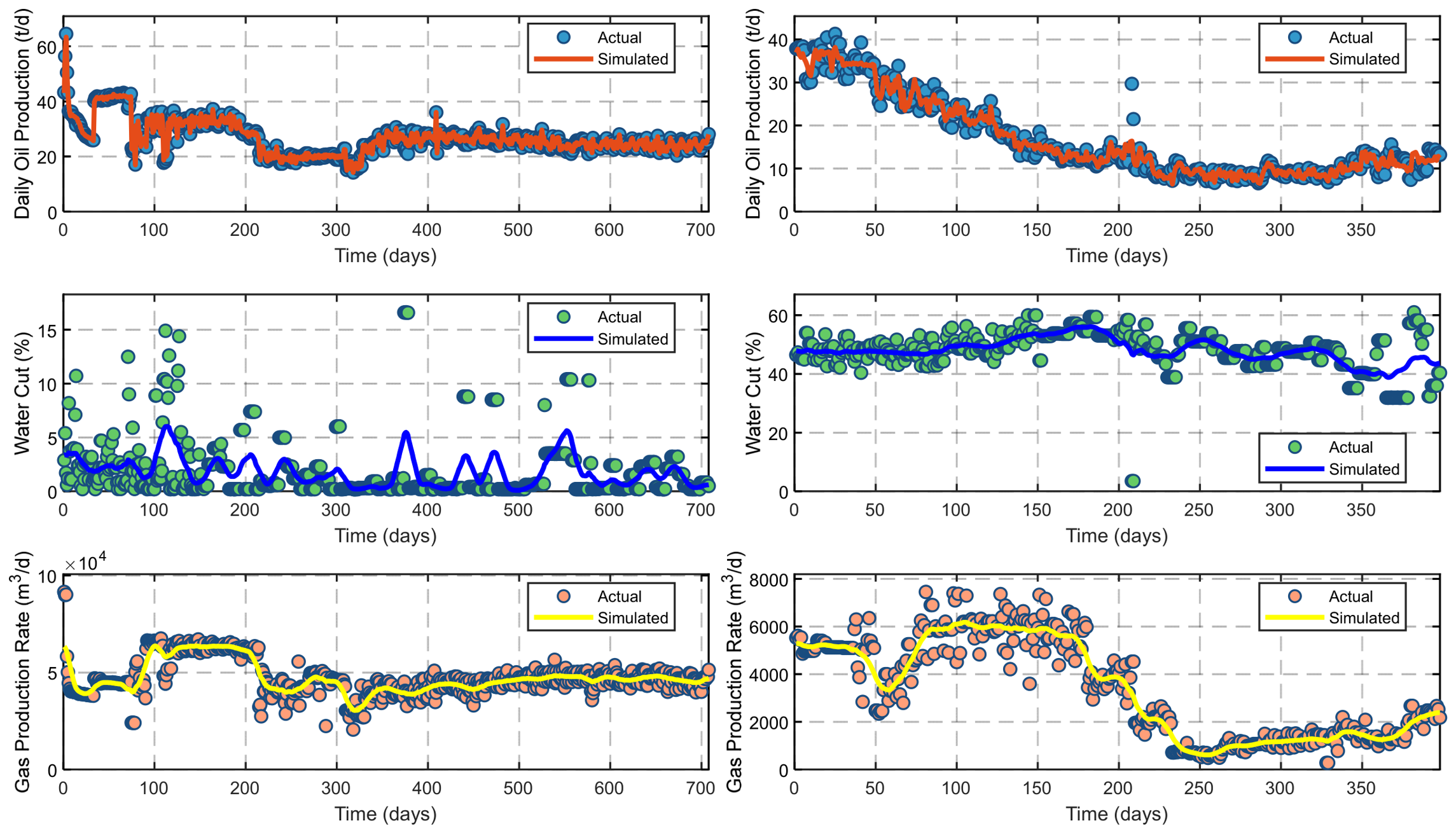
Subsequently, the fracture simulation results were incorporated into the EDFM simulator. By assigning well constraints consistent with the actual field production schedules, the time-dependent variations in the daily oil rate, daily gas rate, and cumulative production of the single well were computed. The simulated production profiles were then compared day-by-day against the actual measured field data. Figure 6 illustrates the history matching curves for the daily oil rate and cumulative oil production of wells HF101H and HF3. It can be observed that the simulated daily oil rates align closely with the measured field data during both the initial decline phase and the subsequent stable production period. Overall, the mean absolute relative errors of the simulated daily oil rates for the two representative wells are 4.7% and 5.1%, respectively, while the relative errors for cumulative oil production remain below 3.0%. The coupled productivity evaluation model constructed in this study demonstrates high predictive accuracy and robust generalization performance during field well data validation. Consequently, it establishes an accurate and reliable data foundation for subsequent dataset generation based on machine learning surrogate models and the analysis of primary controlling factors.

4. Machine Learning-Based Surrogate Model for Productivity Prediction

4.1. Data Characteristics and Preprocessing

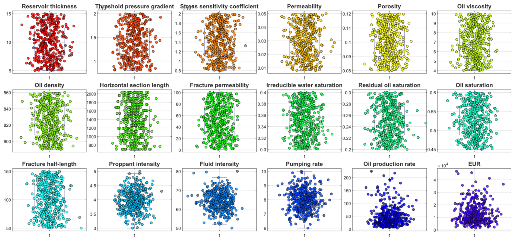
To systematically evaluate the data quality and distribution characteristics of the production dataset, a visualization approach overlaying scatter plots onto box plots is employed to comprehensively analyze the 400 data samples (Figure 7). Scatter plots are utilized to display the raw distribution of all sample points, intuitively illustrating the data density of each parameter. Simultaneously, a corresponding box plot is superimposed above each scatter plot; this box delineates the interquartile range (IQR), median, and potential outliers of the respective parameter. This combined visualization achieves a comprehensive statistical characterization of individual parameter distribution morphologies and dispersion, while enabling the joint observation of parameter-productivity data pairs. Parameters such as permeability and fracture half-length span a wide numerical range and display distinct, positively correlated clouds with productivity; conversely, the threshold pressure gradient exhibits a relatively concentrated distribution. Several box plots reveal the presence of outliers deviating significantly from the main cluster for engineering parameters such as fracturing fluid intensity. Ultimately, this visual analysis provides a crucial distributional foundation for subsequent data preprocessing, feature selection, and model interpretation in machine learning modeling [31].

4.2. Productivity Prediction Surrogate Model

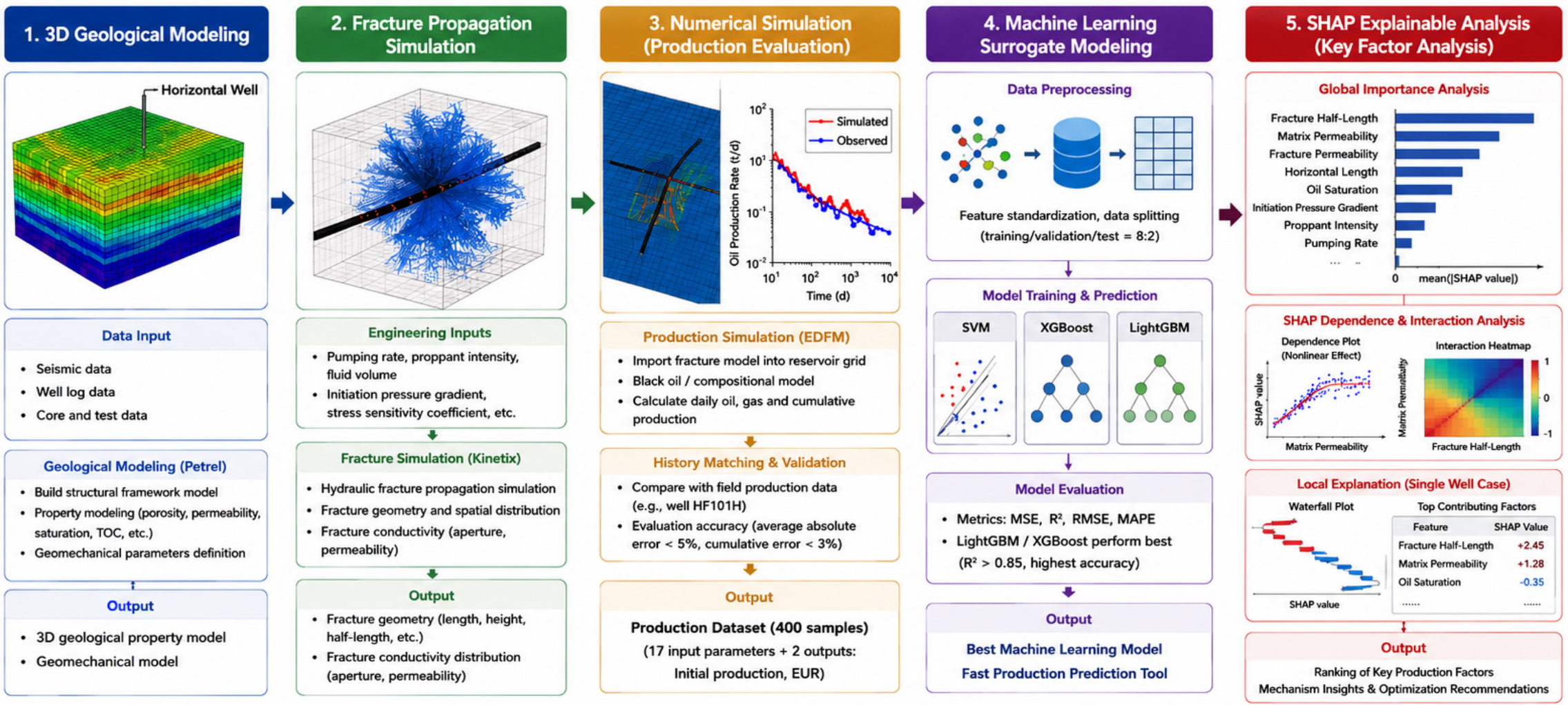
To achieve the rapid identification and quantitative evaluation of the main controlling factors governing the productivity of fractured horizontal wells in tight condensate gas reservoirs, this study establishes an integrated analysis workflow encompassing ‘3D geological modeling–fracture propagation simulation–numerical simulation–machine learning surrogate modeling–SHAP explainable analysis’. This methodology fully integrates the reliability of physics-based models with the efficiency of data-driven models, thereby enhancing the efficiency of productivity analysis and scenario optimization while ensuring high predictive accuracy [32]. Initially, a 3D geological model of the target block is constructed by integrating seismic interpretation, well logs, and core experimental data to capture the spatial distribution characteristics of key geological parameters, including porosity, permeability, oil saturation, and the in situ stress field. Building upon this, a geomechanical parameter model is established via rock mechanics modeling and subsequently imported into hydraulic fracturing simulation platforms to conduct fracture propagation simulations. The simulation process comprehensively accounts for factors such as reservoir heterogeneity, the in situ stress field, and fracturing operational parameters, yielding key fracture attributes including fracture half-length, height, width, and conductivity. Subsequently, the fracture simulation results are coupled with the reservoir geological model, and the EDFM is utilized to construct the productivity prediction model for the fractured horizontal well. The developed model is capable of accurately characterizing the fluid cross-flow process between the fracture and matrix, while incorporating a compositional model to describe the complex phase behavior of the condensate gas reservoir. Utilizing the LHS method, various combinations of geological, engineering, and fluid parameters are generated to perform large-scale numerical simulations, thereby constructing a training dataset that pairs input parameters with their corresponding productivity responses. The primary output metrics of the dataset encompass the initial production rate and the EUR.

Although numerical simulation can accurately capture subsurface flow mechanisms, its calculation process is computationally intensive and time-consuming, making it difficult to meet the demands of large-scale sensitivity analysis and real-time optimization. Consequently, this study introduces a machine learning surrogate model to establish a non-linear mapping relationship between input parameters and productivity indicators, effectively replacing the time-consuming numerical simulations to achieve rapid well-performance prediction.

In this study, four representative machine learning algorithms—namely SVM, RF, XGBoost, and LightGBM—are selected to construct the surrogate models. During the model construction phase, the sample data are first subjected to standardization and then partitioned into training and testing sets according to a specified ratio. Subsequently, the SVM, XGBoost, and LightGBM models are trained respectively. Finally, model performance is rigorously evaluated using metrics such as Mean Squared Error (MSE), Root Mean Squared Error (RMSE), Mean Absolute Percentage Error (MAPE), and the coefficient of determination (R²). By comparing the predictive results of the different algorithms, the best-performing surrogate model is selected for subsequent interpretive analysis. Upon establishing this high-accuracy surrogate model, the SHAP framework is further introduced to conduct both global and local interpretations of the model’s predictions, as shown in Figure 8. Rooted in the Shapley value theory from cooperative game theory, the SHAP method quantitatively evaluates the contribution of each input feature to the model’s predictions. Through global importance ranking, SHAP dependence plots, and feature interaction analysis, it not only identifies the crucial geological and engineering parameters governing well productivity but also unveils the underlying non-linear relationships and synergistic mechanisms among these variables.

4.3. Machine Learning Models

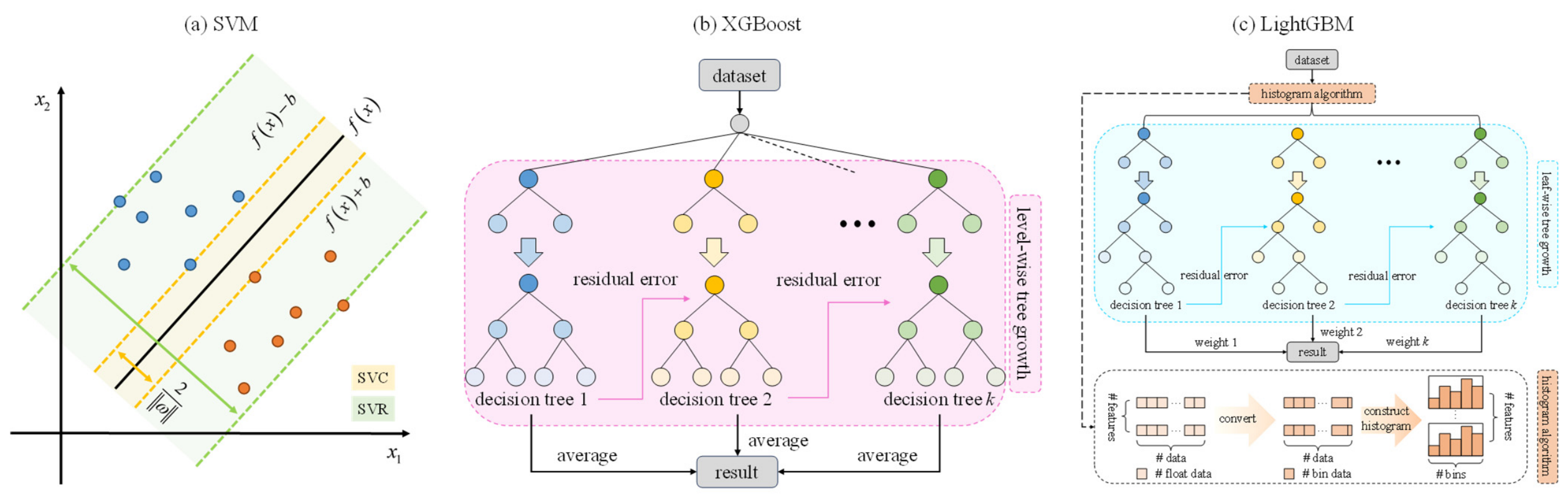
SVM is a supervised learning model that encompasses both classification and regression variants, namely Support Vector Classification (SVC) and Support Vector Regression (SVR). It exhibits excellent robustness and adaptability when addressing non-linear regression challenges, as shown in Figure 9a. The fundamental objective of such regression tasks is to fit the dataset by constructing a mapping function that minimizes the error between the predicted values and the ground truth [33]. In conventional regression, the loss becomes zero only when the ground truth $f\left(x\right)$ and the predicted value $y$ are perfectly identical. In contrast, when a Support Vector Machine is applied to regression tasks, its objective is to identify a hyperplane that minimizes the distance between the training data points and this hyperplane within a predefined margin of tolerance $ϵ$. Specifically, the loss is calculated only when the condition $\left|\mathrm{f}\left(\mathrm{x}\right)-\mathrm{y}\right|>\mathsf{ϵ}$ is satisfied. This is equivalent to constructing an insensitive band (or tube) with a width of $2ϵ$, centered around $\mathrm{f}\left(\mathrm{x}\right)=\mathsf{\omega }·\mathrm{x}+\mathrm{b}$. If a training sample falls inside this band, the prediction is considered correct, yielding zero loss. The optimal hyperplane is determined by minimizing a loss function equipped with a tolerance threshold and a regularization term. This optimization objective can be formulated as a minimization problem with a penalty function. Typically, a loss function incorporating either L1 or L2 regularization is adopted to control model complexity. The target objective function to be minimized can be expressed as:

$$SV{M}_{-}Loss=\underset{\omega ,b}{\min }{\displaystyle \frac{1}{2}}\parallel \omega {\parallel }^2+C{\displaystyle \sum _{i=1}^n}{L}_{\epsilon }(y_i,\omega \cdot x_i+b)$$

(12)

where $\omega$ is the normal vector of the hyperplane; $i$ is the data index; $n$ denotes the total number of training samples; C is the regularization parameter; $L_{\epsilon }$ represents the loss function; $y_i$ is the true label; and $b$ denotes the width of the “margin band”, acting as the penalty term, which typically serves to penalize model complexity.

XGBoost is an ensemble learning method based on the gradient boosting framework. Its base learners are decision trees; by combining multiple base learners, it iteratively corrects the errors of the preceding model in each round, thereby constructing a robust and powerful model. The primary distinction between XGBoost and Random Forest lies within their specific model training mechanisms. The former sequentially adds a new tree at each step based on the previous one, and this newly incorporated tree is specifically designed to rectify the shortcomings of the preceding model. Its fundamental structure is illustrated in Figure 9b. By explicitly incorporating the complexity of the tree models into the regularization term, XGBoost demonstrates exceptional performance in mitigating overfitting and enhancing generalization capabilities. The algorithm trains the model by minimizing the sum of weighted residuals. The comprehensive loss function comprises a prediction error term and a regularization penalty term. The primary objective of XGBoost is to minimize this objective function, which is generally formulated as follows:

$$XGBoos{t}_{-}Loss={\displaystyle \sum _{i=1}^n}L(y_i,{\widehat{y}}_i)+{\displaystyle \sum _{k=1}^K}\mathsf{\Omega }(f_k)$$

(13)

where $n$ represents the number of training samples; ${\widehat{y}}_i$ denotes the predicted value; $L\left(y_i,{\widehat{y}}_i\right)$ denotes the loss function, which is typically configured as the MSE; and $\mathsf{\Omega }\left(f_k\right)$ is the regularization term for the decision tree $f_k$, which is employed to control model complexity and mitigate overfitting.

LightGBM shares a conceptual lineage with XGBoost, both being ensemble architectures underpinned by the gradient boosting mechanism, as schematically depicted in Figure 9c. While XGBoost is capable of locating exact splitting points through its meticulous pre-sorting approach, this deterministic precision often incurs a prohibitive computational overhead, an intensive memory footprint, and a heightened susceptibility to overfitting. To overcome these limitations, LightGBM utilizes a histogram-based optimization learning method and a leaf-wise tree growth strategy, while concurrently supporting feature parallelization. This configuration significantly curtails the number of candidate split points and the corresponding memory footprint, drastically accelerates computational velocity, and effectively mitigates the risk of overfitting. During the training phase, unlike conventional GBDT algorithms that necessitate exhaustive multiple traversals of the entire dataset, LightGBM utilizes residual gradients by feeding the output of the preceding iteration as the direct input for the subsequent one. Fundamentally, LightGBM executes decision tree splitting via a histogram-based algorithm coupled with a depth-constrained leaf-wise growth strategy. It discretizes continuous feature values into distinct bins, subsequently constructing the functional histograms to optimize the split evaluation. Specifically, LightGBM replaces the traditional level-wise tree growth scheme with a depth-constrained leaf-wise (best-first) growth strategy. Compared to the level-wise expansion adopted by XGBoost, this leaf-wise approach drastically minimizes the computational overhead associated with searching for optimal split points. By curbing redundant calculations, the mechanism renders LightGBM exceptionally efficient in terms of memory footprint while robustly circumventing the risk of overfitting when regulated by structural depth constraints. Feature parallelization serves as a highly effective mechanism for processing high-dimensional data, allowing each computational unit to focus exclusively on a specific subset of features. Adhering to a robust parallel computing paradigm, LightGBM partitions the dataset across multiple distributed nodes. These nodes process their assigned features concurrently to find the local optimal splits, after which the global model parameters are updated by synchronizing and merging the local outputs from each individual node. Additionally, LightGBM incorporates k-fold cross-validation to rigorously assess model performance, supplemented by an early stopping mechanism that automatically halts the training process once the generalization metrics on the validation set cease to improve, thereby robustly suppressing overfitting. In practical deployment, since LightGBM progressively refines the tree architectures through successive iterations, meticulous hyperparameter tuning tailored to the specific database characteristics and learning objectives is paramount to unlocking its peak predictive capacity.

4.4. Model Training Strategy

To ensure unbiased performance evaluation and rigorous hyperparameter tuning, the entire dataset (400 samples) was initially split into two distinct subsets via stratified random sampling: a training set comprising 80% (320 samples) and an independent test set comprising 20% (80 samples). The test set was strictly withheld from all training and validation processes, serving exclusively as the final hold-out benchmark to evaluate the generalization capability of the optimally tuned models.

For hyperparameter optimization, a 5-fold cross-validation strategy was exclusively applied to the 320 training samples. Specifically, the training set was randomly partitioned into 5 equal-sized folds. For each candidate hyperparameter combination during the grid search, the model was trained on 4 folds and validated on the remaining 1 fold; this procedure was cycled 5 times until every fold had been used exactly once as the validation set. The average RMSE across the 5 validation folds was adopted as the primary metric for selecting the optimal hyperparameters. The hyperparameter selections for the four models are shown in

Table 2. The hyperparameter selections for the four models.

Model	Hyperparameter	Search Range	Optimal Value
SVM (SVR)	Kernel function	linear, rbf, poly	rbf
	Regularization parameter (C)	[0.1, 1, 10, 100]	10
	Epsilon (ε)	[0.001, 0.01, 0.1]	0.01
	Gamma (γ)	[0.001, 0.01, 0.1, 1]	0.1
Random Forest (RF)	Number of trees (n_estimators)	[50, 100, 200, 300]	150
	Max depth	[5, 10, 20, None]	20
	Min samples split	[2, 5, 10]	2
	Min samples leaf	[1, 2, 4]	1
	Max features	[‘sqrt’, ‘log2’, None]	‘sqrt’
XGBoost	Number of trees (n_estimators)	[50, 100, 200, 300]	200
	Learning rate (eta)	[0.01, 0.05, 0.1, 0.2]	0.1
	Max depth	[3, 6, 9, 12]	6
	Subsample	[0.6, 0.8, 1.0]	0.8
	Colsample_bytree	[0.6, 0.8, 1.0]	0.8
	L1 regularization (alpha)	[0, 0.1, 1]	0.1
	L2 regularization (lambda)	[0, 0.1, 1]	1
LightGBM	Number of trees (n_estimators)	[50, 100, 200, 300]	200
	Learning rate	[0.01, 0.05, 0.1, 0.2]	0.1
	Num leaves	[7, 15, 31, 63]	31
	Max depth	[5, 10, 15, −1]	10
	Subsample (bagging_fraction)	[0.6, 0.8, 1.0]	0.8
	Colsample_bytree (feature_fraction)	[0.6, 0.8, 1.0]	0.8
	L1 regularization (reg_alpha)	[0, 0.1, 1]	0.1
	L2 regularization (reg_lambda)	[0, 0.1, 1]	1

.

After the optimal hyperparameters were identified for each algorithm, the final surrogate model was retrained on the complete training set and then evaluated once on the untouched test set to report the final predictive performance. This strict separation guarantees that the reported metrics reliably reflect the models’ true predictive power on unseen data without any optimistic bias.

5. Results

5.1. Analysis of Factors Influencing Productivity

5.1.1. Influence of Matrix Permeability

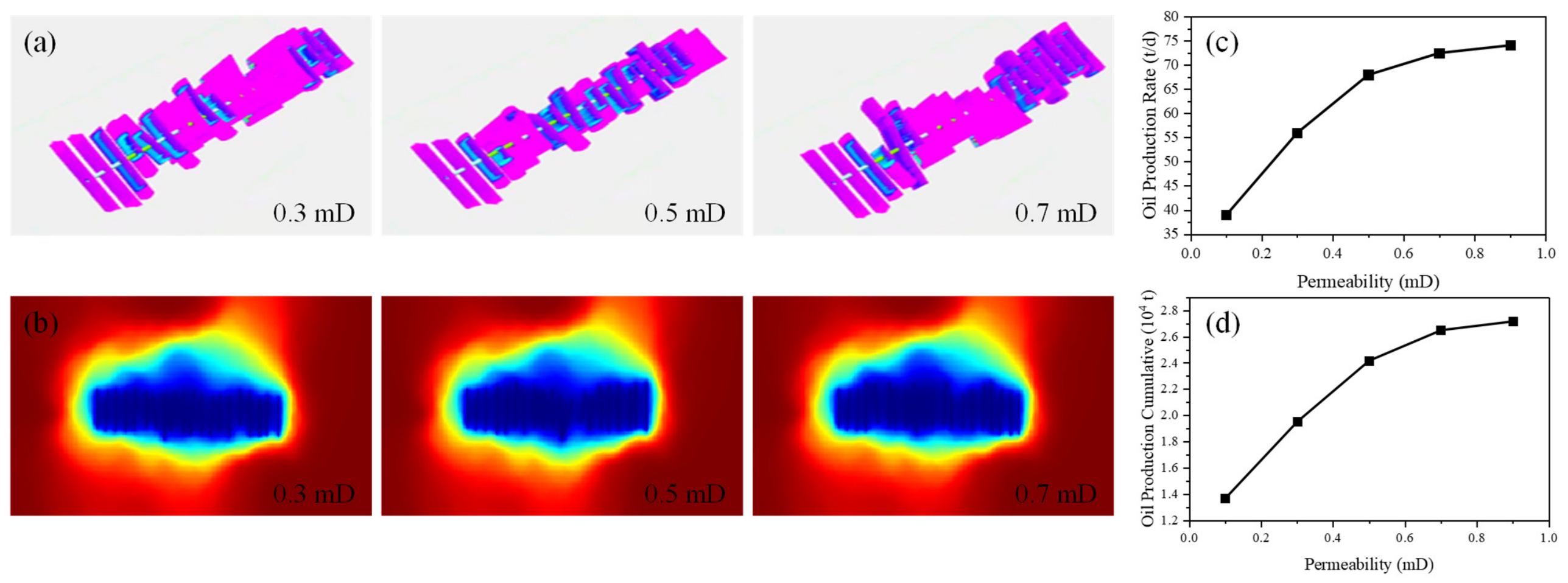
Matrix permeability is a critical geological parameter characterizing the fluid flow capacity of a reservoir. Its magnitude not only directly governs the hydrocarbon supply efficiency from the matrix into the fracture network but also indirectly impacts the ultimate geometry of hydraulic fractures by altering the stress distribution and fluid leak-off behavior during fracture propagation. Based on the established integrated geological-engineering production evaluation model, five scenarios were designed with matrix permeabilities of 0.1 mD, 0.3 mD, 0.5 mD, 0.7 mD, and 0.9 mD, while holding all other parameters constant. This approach enables a systematic analysis of how matrix permeability influences hydraulic fracture propagation and the productivity of fractured horizontal wells.

Figure 10 compares the initial production and cumulative oil production of the fractured horizontal well under different matrix permeabilities. The results indicate that the initial production exhibits a non-linear increase with rising matrix permeability: as the permeability increases from 0.1 mD to 0.3 mD, the initial production is enhanced by approximately 48%; however, as the permeability rises from 0.7 mD to 0.9 mD, this increment margin drops to 12%. This trend underscores the heightened sensitivity of well productivity to low-permeability conditions. Within the ultra-low permeability regime, marginal improvements in permeability can trigger a substantial surge in production. However, once the permeability surpasses 0.5 mD, further productivity growth is primarily constrained by the matching relationship between fracture conductivity and fluid supply. Regarding cumulative oil production, its variation trend is largely consistent with that of the initial production. However, during the late stages of production, the advantage in cumulative yield for high-permeability cases becomes increasingly pronounced. This indicates that the controlling effect of matrix permeability on long-term development performance amplifies as production time extends.

5.1.2. Influence of Injection Rate

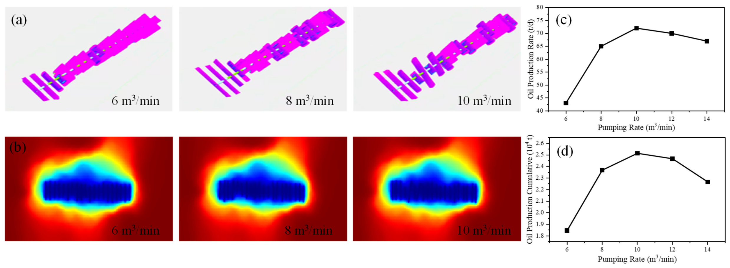
The pumping rate is a critical, directly controllable engineering parameter in hydraulic fracturing operations. Its magnitude dictates the fracturing fluid injection rate, net pressure within the fractures, and proppant transport efficiency, thereby influencing the ultimate fracture geometries, conductivity distributions, and overall production performance. To quantify the impact of the pumping rate, five simulation scenarios were established with pumping rates set at 6 m³/min, 8 m³/min, 10 m³/min, 12 m³/min, and 14 m³/min, while holding all other parameters constant. Figure 11 illustrates the impacts of selected parameters on the productivity of fractured horizontal wells. As the pumping rate increases, the net pressure within the fracture rises significantly, thereby enhancing the fracture propagation capability in both the length and height directions. At a pumping rate of 8 m³/min, the fracture half-length is approximately 142 m with an average fracture width of 1.5 mm. When the pumping rate is elevated to 10 m³/min, the fracture half-length increases to 198 m (an increment of ~39%), and the average fracture width reaches 2.2 mm (a growth of ~47%). Concurrently, the fracture height also exhibits an upward trend, albeit with a relatively minor increment. This implies that under the specific in situ stress conditions of the study area, the elevated net pressure is preferentially consumed to drive the lateral propagation of the fracture rather than significantly increasing its height. This behavior is highly favorable for achieving comprehensive vertical reservoir stimulation during multistage horizontal well fracturing operations. The initial production exhibits non-linear growth with an increasing pumping rate; however, both the initial production and cumulative oil yield decline once the rate surpasses 10 m³/min. This inflection indicates that an excessively high pumping rate aggravates proppant-induced erosion on the fracture walls and intensifies localized accumulation, triggering varying degrees of sand-plugging that restricts the effective fracture length. Consequently, for the tight condensate gas reservoir in block HF3 of the study area, an optimized pumping rate interval of 8–12 m³/min is recommended, within which a superior trade-off between productivity gains and economic returns can be achieved.

5.2. Machine Learning Model Prediction Results

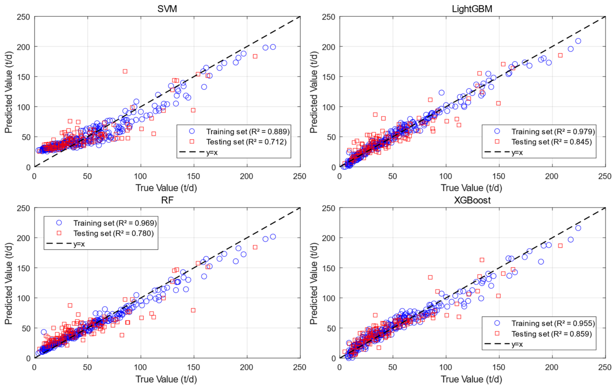
Building upon the algorithms detailed in Section 4.3, three distinct surrogate models—SVM, LightGBM, and XGBoost—were developed for well-productivity forecasting. The prediction results are shown in Figure 12. To comprehensively evaluate and compare the predictive capabilities of these candidate models, four statistical metrics were employed: MSE, R2, RMSE, and MAPE. The forecasting results demonstrate that all three candidate models exhibit robust learning capacities, yielding a high level of overall predictive accuracy. Specifically, the prediction accuracies are logged at 71.3%, 68.4%, 80.9%, and 86.3%, respectively, among which the LightGBM algorithm achieves the peak predictive performance. Nevertheless, notable performance discrepancies exist: LightGBM and XGBoost significantly outperform SVM regarding predictive accuracy on the testing set. Their RMSE is reduced by approximately 30% on average, with the R², exceeding 0.85. This distinctly highlights the inherent advantages of tree-based ensemble models in processing high-dimensional and non-linearly structured data. Specifically, XGBoost exhibits the highest stability in predicting the EUR, whereas LightGBM holds a conspicuous advantage in terms of computational efficiency during the training phase. Although the SVM model provides relatively higher model transparency, its overall forecasting precision remains constrained, particularly underperforming when fitting extreme high-value samples. Consequently, a comprehensive trade-off evaluation suggests that LightGBM and XGBoost serve as more competent benchmark architectures for the subsequent SHAP-based interpretability analysis.

6. SHAP-Based Analysis of Factors Influencing Productivity

6.1. Correlation Analysis

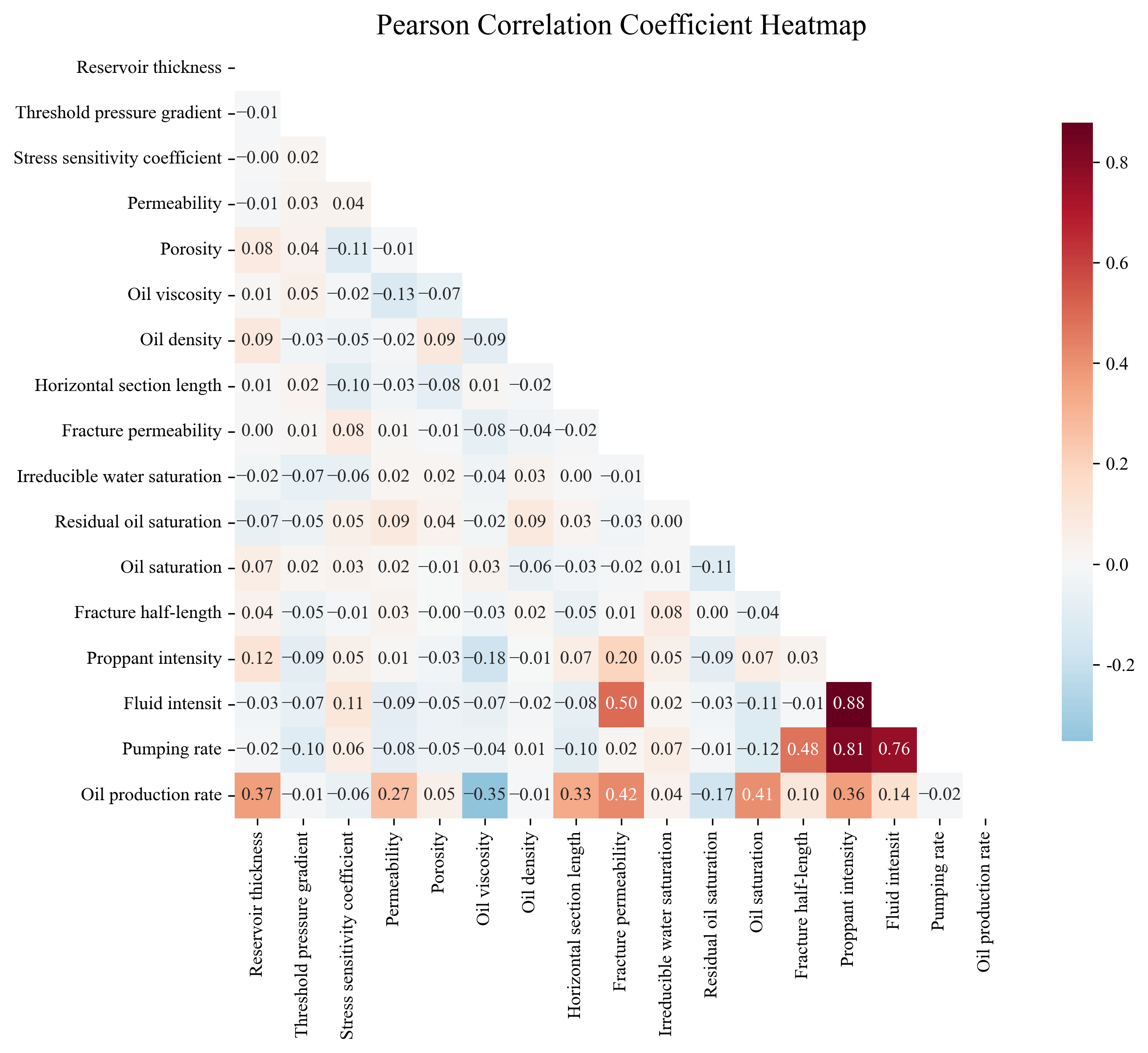
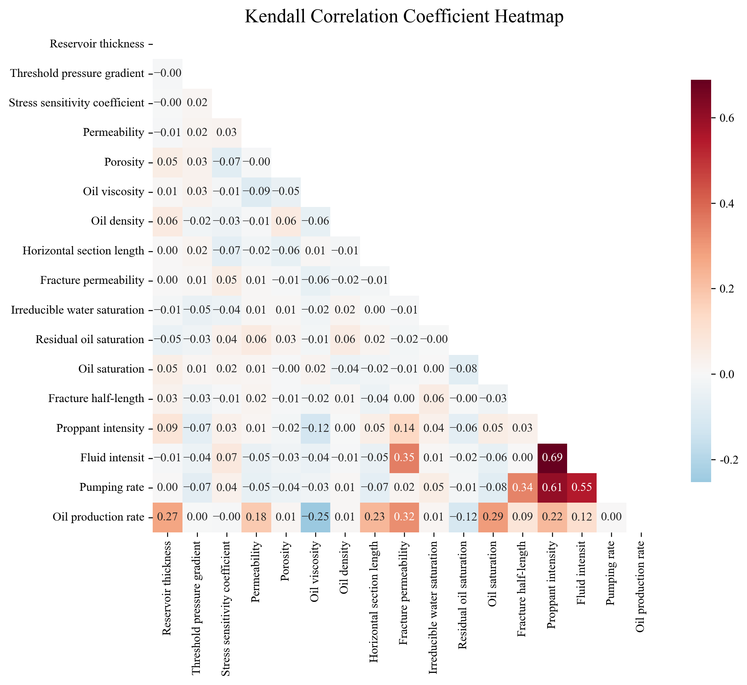
Following the successful deployment of the three machine learning architectures for well-productivity forecasting, this study conducted an independent and quantitative statistical assessment to evaluate the direct impact of individual variables on production capacity. Specifically, a comprehensive correlation evaluation encompassing all 16 influencing factors was initially performed utilizing Pearson, Spearman rank, and Kendall rank correlation coefficients. The mathematical formulation of the Pearson correlation coefficient is expressed as follows:

$$r={\displaystyle \frac{{\displaystyle \sum _{i=1}^n(x_i-\overline{x})}(y_i-\overline{y})}{\sqrt{{\displaystyle \sum _{i=1}^n{(x_i-\overline{x})}^2}}\sqrt{{\displaystyle \sum _{i=1}^n{(y_i-\overline{y})}^2}}}}$$

(14)

where $x_i$ and $y_i$ denote the i-th pair of sample values; $\overline{x}$ and $\overline{y}$ represent their respective sample means; and n indicates the total sample size.

The mathematical formulation for the Spearman rank correlation coefficient is given by:

$$\rho =1-{\displaystyle \frac{6{\displaystyle \sum _{i=1}^n}{d}_i^2}{n(n^2-1)}}$$

(15)

where $d_i=R\left(x_i\right)-R\left(y_i\right)$ denotes the rank difference between the two variables; $R\left(x_i\right)$ represents the specific rank of $x_i$ within the $x$ sequence; and $n$ is the total sample size.

The mathematical formulation for the Kendall rank correlation coefficient is given by:

$${\tau }_b={\displaystyle \frac{n_c-n_d}{\sqrt{(n_c+n_d+t_x)(n_c+n_d+t_y)}}}$$

(16)

where $n_c$ is the number of concordant pairs; $n_d$ is the number of discordant pairs; $t_x={\sum }_k{\displaystyle \frac{t_{xk}\left(t_{xk}-1\right)}{2}}$, where $t_{xk}$ is the number of values in the $k$-th tied group of $x$; and $t_y$ is defined similarly to $t_x$.

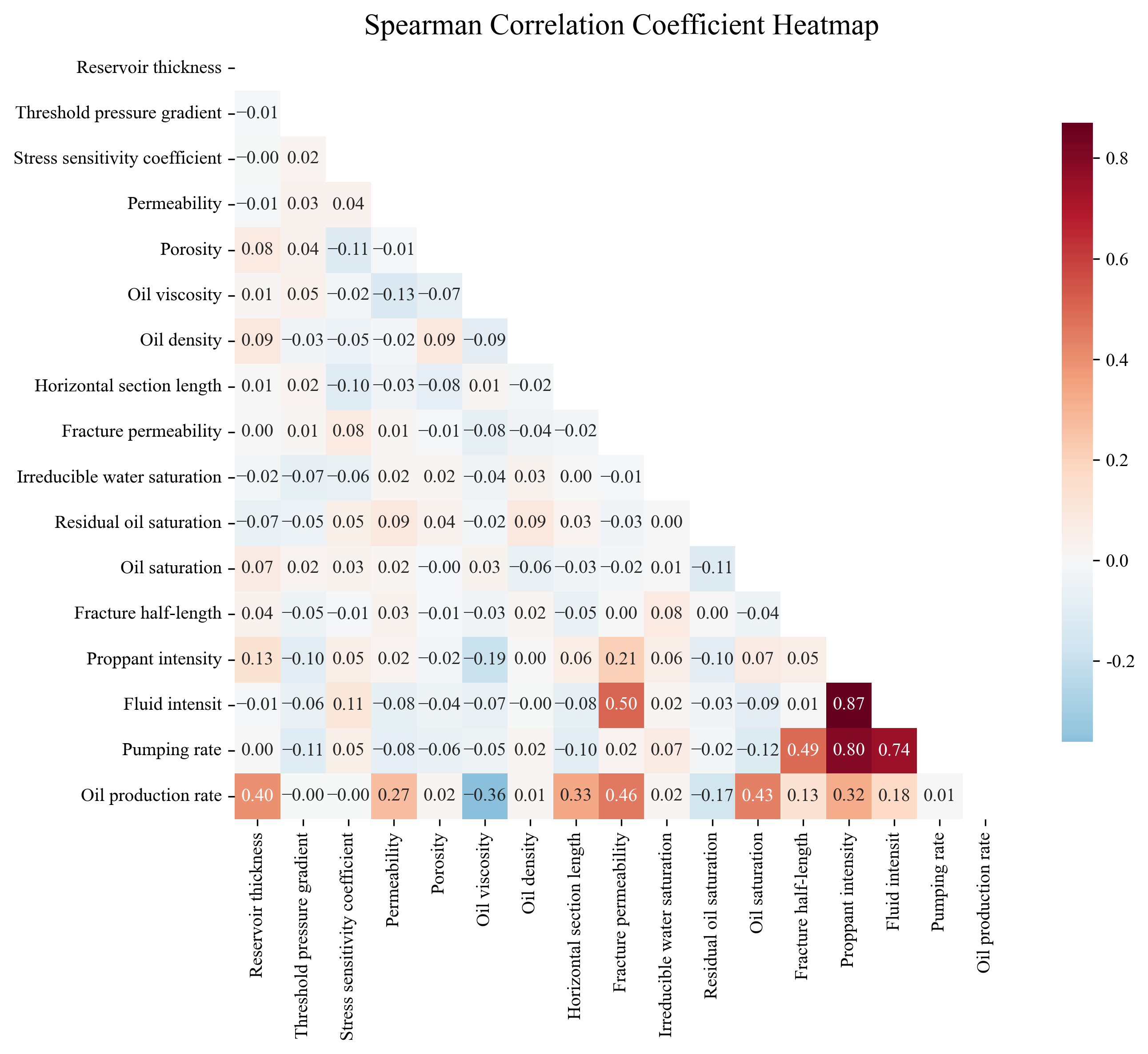
The analytical results are visualized via a heatmap, as depicted in Figure 13. The Pearson correlation coefficient is specifically employed to quantify the magnitude and direction of the linear associations among the variables. The analytical results reveal that fracture half-length, fracture permeability, and lateral length exhibit significant positive linear correlations with both productivity indicators. This underscores that expanding fracture dimensions and maximizing the reservoir-wellbore contact area serve as direct and effective engineering levers to enhance well productivity. In contrast, the Spearman and Kendall rank correlation coefficients prioritize the evaluation of monotonic relationships and exhibit inherent robustness against non-normal data distributions and outliers. The conclusions derived from these two non-parametric metrics are highly congruent. They not only corroborate the aforementioned strongly correlated linear factors but, more importantly, unveil a robust positive monotonic relationship between key reservoir parameters and well productivity. Despite yielding relatively subdued Pearson coefficients, these variables possess substantial potential for non-linear contributions to the forecasting models.

A comprehensive synthesis of the three evaluation metrics reveals that fracture parameters consistently maintain a dominant position across all correlation assessments. Concurrently, reservoir quality serves as the foundational geological core dictating the intrinsic production potential. In stark contrast, crude oil properties and certain well completion parameters exhibit relatively marginal correlations within the confines of the present dataset. Consequently, this statistical analysis establishes a vital a priori knowledge reference and a robust validation foundation for the ensuing machine learning-driven SHAP interpretability analysis.

6.2. SHAP-Based Analysis of Main Controlling Factors for Well Productivity

Following the baseline statistical characterization, this study further leverages the SHAP approach to execute a rigorous interpretability analysis on the optimal machine learning architecture [34]. This implementation aims to thoroughly unravel the non-linear influence mechanisms, interaction effects, and individual feature contributions governing the productivity of fractured horizontal wells. The SHAP-based diagnostic framework is deployed across both global and local dimensions, with its foundational mathematical formulation expressed as follows:

$${\varphi }_i=\sum _{S\subseteq F\setminus \left\{i\right\}}{\displaystyle \frac{\left|S\right|!(|F|-|S|-1)!}{\left|F\right|!}}\left[f(S\cup \{i\})-f(S)\right]$$

(17)

where ${\varphi }_i$ represents the SHAP value of feature $i$; F denotes the universal set of all input features; S indicates a subset of features that excludes feature $i$; f(S) represents the model’s prediction output conditioned exclusively on the features within subset $S$; and f(S∪{i}) signifies the prediction output after integrating feature $i$ into subset $S$.

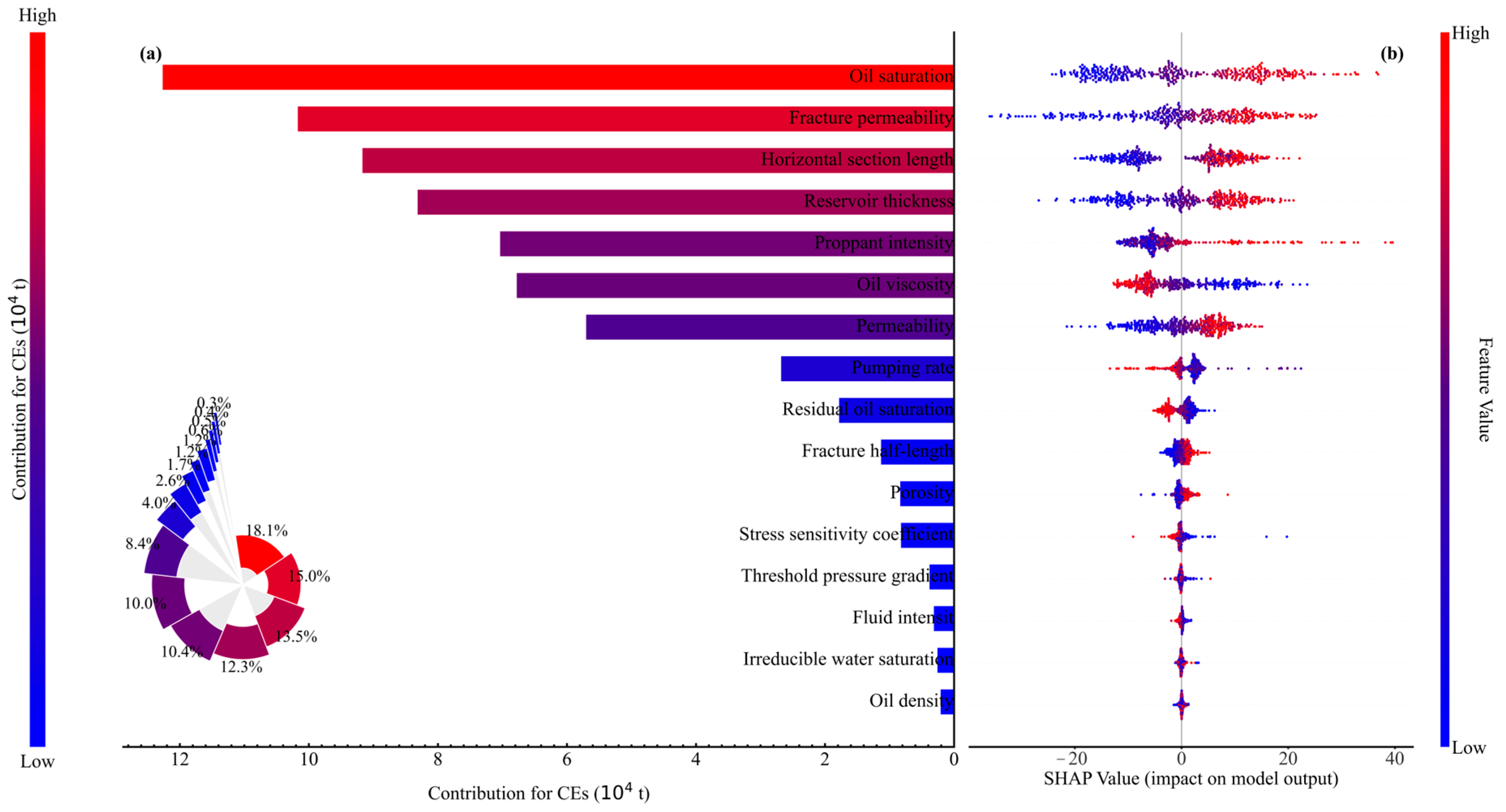
By computing the SHAP values for various parameters and visualizing them via bar plots and scatter plots (as depicted in Figure 14), the global feature importance was successfully quantified. The global importance analysis demonstrates that fracture half-length, matrix permeability, and fracture permeability constitute the top three most critical factors dictating well productivity. Their mean absolute SHAP values are prominently higher than those of the remaining parameters. This finding strongly corroborates the insights from the prior statistical correlation analysis while delivering a more rigorous and precise feature ranking [35]. Crucially, the SHAP dependence plots elucidate the profound non-linear underlying mechanisms of these core parameters: the positive contribution of fracture half-length to well productivity exhibits a distinct critical threshold characterized by “diminishing returns.” Concurrently, an enhancement in matrix permeability within the low-value regime triggers an exponential surge in production capacity; however, upon surpassing a specific threshold, its marginal utility attenuates significantly. Furthermore, the SHAP interaction value analysis uncovers pivotal feature synergistic effects. As illustrated in Figure 14, a robust positive interaction manifests between fracture half-length and matrix permeability. Specifically, under conditions of elevated reservoir permeability, the promotional effect of increasing fracture half-length on well productivity is significantly amplified. In stark contrast, certain engineering parameters and geological characteristics exhibit distinct mutual constraints.

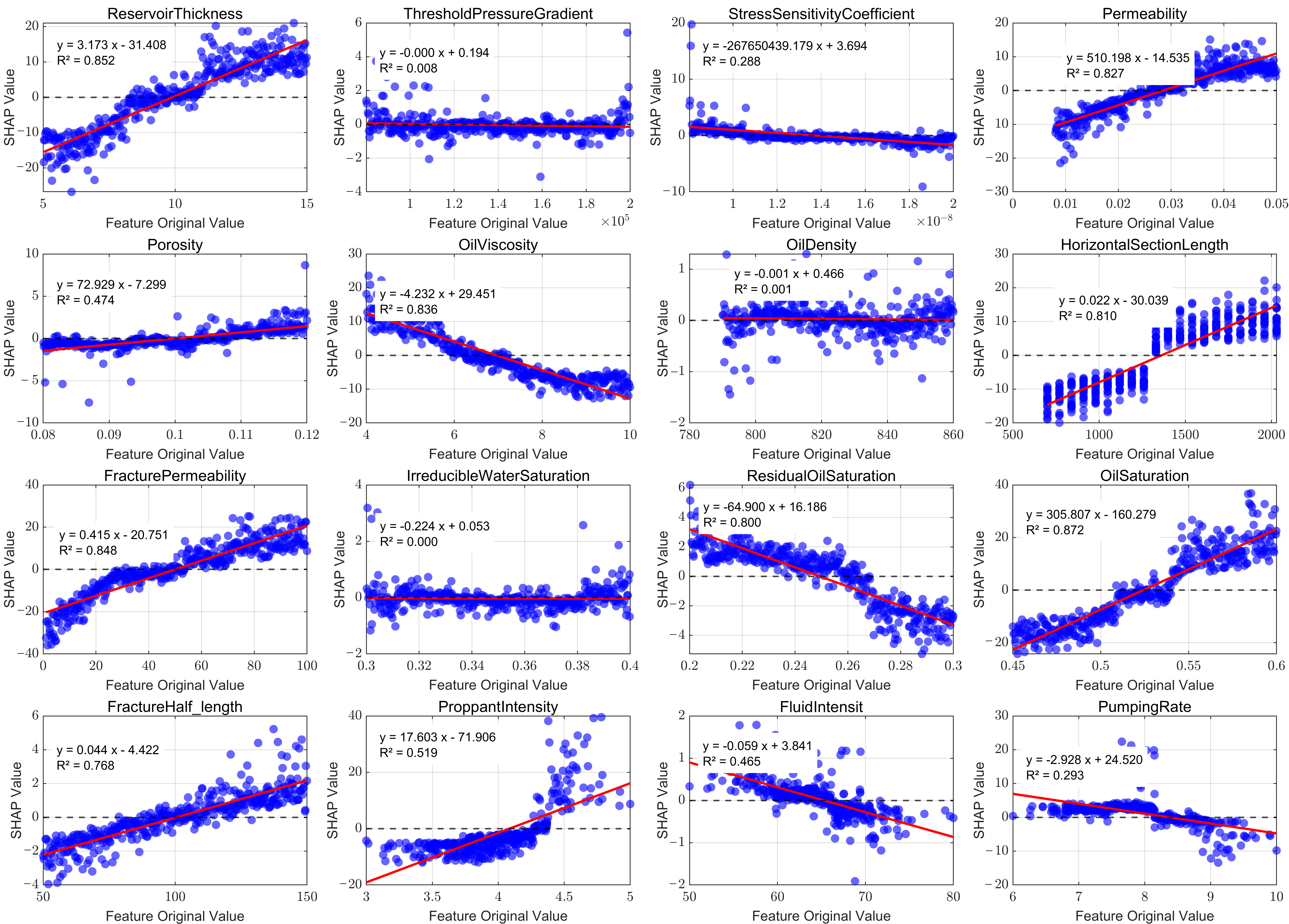
Furthermore, the underlying relationship between the raw feature values and their corresponding SHAP values was systematically analyzed, with the results visually presented via scatter plots in Figure 15. The correlation between input features and SHAP values serves as a potent tool for deciphering black-box model behaviors, as it effectively unravels the directionality, magnitude, and degree of linearity of the feature impacts. When a strong positive correlation exists between a feature’s raw values and its SHAP values, larger feature magnitudes correspond to higher SHAP values, signifying a positive contribution to the model’s predictive output. Furthermore, a greater absolute slope of the fitted regression line indicates a more drastic shift in the SHAP value per unit change in the feature, thereby implying that the model exhibits heightened sensitivity to this specific parameter. As clearly evidenced in Figure 15, oil saturation, fracture permeability, lateral length, and reservoir thickness exert substantial contributions to the model output, standing out as the primary control factors governing well productivity; this aligns closely with the global insights derived from Figure 14. Regarding the operational parameters, the displacement rate exhibits a marginal positive contribution when maintained below 8 m³/min, but transitions to an adverse contribution once surpassing this threshold, which strongly corroborates the physical trends demonstrated in Figure 8. Conversely, local explanations cater to single-well predictions by quantifying the precise contribution magnitude and directional impact of each feature, thereby providing a transparent attribution tool for the diagnostic analysis of anomalous individual wells with exceptionally high or low production. Ultimately, the SHAP framework not only quantitatively reinforces the dominant control of reservoir and engineering parameters but also profoundly dissects their intricate non-linear relationships and synergistic mechanisms. This methodology successfully transforms the machine learning “black-box” model into interpretable and verifiable engineering decision-making knowledge, delivering profound insights that transcend conventional statistical paradigms to facilitate targeted hydraulic fracturing optimization.

7. Conclusions

Targeting the core objective of precisely identifying and quantitatively evaluating the primary productivity-controlling factors for fractured horizontal wells in tight condensate gas reservoirs, this study systematically formulates and executes a comprehensive “geology–fracturing simulation–productivity prediction–machine learning–interpretability analysis” integrated research paradigm. By seamlessly integrating geological modeling, hydraulic fracturing simulation, EDFM-based numerical reservoir simulation, and multi-dimensional data analytics, the following primary conclusions have been established:

(1) The integrated workflow effectively bridges the entire technical pipeline from geological characterization to production decision-making. The high-fidelity 3D geomechanical models and fracture propagation simulations, developed via Petrel and Kinetix, lay a robust physical foundation for the subsequent productivity analysis. Furthermore, the EDFM approach successfully accomplishes high-efficiency fluid flow simulation within intricate fracture networks, yielding predictive datasets that constitute a robust sample repository for the ensuing data-driven analytics.

(2) Machine learning-based surrogate models exhibit remarkable superiority in well-productivity forecasting. In predictive tasks leveraging a dataset of 400 geological and engineering parameter combinations, tree-based ensemble models achieved a predictive accuracy (R² > 0.85) significantly superior to that of SVM. This remarkable performance substantiates their exceptional adaptability and robustness in processing high-dimensional, non-linear reservoir development data, ultimately establishing them as highly efficient proxies capable of replacing computationally expensive numerical simulations.

(3) The SHAP interpretability framework successfully elucidates the intricate underlying mechanisms governing the primary productivity-controlling factors.

(4) This study explicitly delineates the pathways for the synergistic optimization of the geological foundation and engineering parameters. Specifically, well productivity is not dictated by an isolated engineering parameter; rather, it is the definitive manifestation of a synergistic interplay between reservoir quality and hydraulic fracture engineering. The efficacy of engineering optimization is heavily contingent upon the underlying geological context, and single-mindedly maximizing a standalone engineering index often precipitates a sharp decline in marginal utility. Consequently, engineering personalized hydraulic fracturing designs that achieve geological matching is paramount to unlocking the full potential of reservoir development performance.

References

1. Bai, W.; Cheng, S.; Wang, Y.; Cai, D.; Guo, X.; Guo, Q. A transient production prediction method for tight condensate gas wells with multiphase flow. Pet. Explor. Dev. 2024, 51, 2–10. [Google Scholar] [CrossRef]
2. Zhu, H.; Jin, X.; Guo, J.; An, F.; Wang, Y.; Lai, X. Coupled flow, stress and damage modelling of interactions between hydraulic fractures and natural fractures in shale gas reservoirs. Int. J. Oil Gas. Coal Technol. 2016, 13, 359–390. [Google Scholar] [CrossRef]
3. Tu, H.; Zhang, R.; Guo, P.; Hu, S.; Peng, Y.; Ji, Q.; Li, Y. The Impact of Condensate Oil Content on Reservoir Performance in Retrograde Condensation: A Numerical Simulation Study. Energies 2024, 17, 5750. [Google Scholar] [CrossRef]
4. Cheng, Y. Mechanical interaction of multiple fractures-exploring impacts of the spacing/number of perforation clusters on horizontal shale-gas wells. SPE J. 2012, 17, 4–1001. [Google Scholar] [CrossRef]
5. Ma, X.; Hou, M.; Zhan, J.; Liu, Z. Interpretable Predictive Modeling of Tight Gas Well Productivity with SHAP and LIME Techniques. Energies 2023, 16, 3653. [Google Scholar] [CrossRef]
6. Rahmanifard, H.; Gates, I. Innovative integrated workflow for data-driven production forecasting and well completion optimization: A Montney Formation case study. Geoenergy Sci. Eng. 2024, 238, 212899. [Google Scholar] [CrossRef]
7. Kim, S.; Kim, K.; Lim, J. Synergistic Enhancement of Productivity Prediction Using Machine Learning and Integrated Data from Six Shale Basins of the USA. Geoenergy Sci. Eng. 2023, 229, 212068. [Google Scholar] [CrossRef]
8. Zhai, S.; Geng, S.; Li, C.; Gong, Y.; Jing, M.; Li, Y. Prediction of gas production potential based on machine learning in shale gas field: A case study. Energy Sources Part A Recovery Util. Environ. Eff. 2022, 44, 6581–6601. [Google Scholar]
9. Bhattacharyya, S.; Vyas, A. Application of Machine Learning in Predicting Oil Rate Decline for Bakken Shale Oil Wells. Sci. Rep. 2022, 12, 16154. [Google Scholar] [CrossRef] [PubMed]
10. Wu, M.; Li, H.; Mao, Y. An automatic three-dimensional geological engineering modeling method based on tri-prism. Arab. J. Geosci. 2020, 13, 358. [Google Scholar] [CrossRef]
11. Chen, H.; Liu, H.; Shen, C.; Xie, W.; Liu, T.; Zhang, J.; Lu, J.; Li, Z.; Peng, Y. Research on Geological-Engineering Integration Numerical Simulation Based on EUR Maximization Objective. Energies 2024, 17, 3644. [Google Scholar] [CrossRef]
12. Zeng, J.; Li, W.; Fang, H.; Huang, X.; Wang, T.; Zhang, D.; Yuan, S. The hydraulic fracturing design technology and application of geological-engineering integration for tight gas in jinqiu gas field. Front. Energy Res. 2022, 10, 1003660. [Google Scholar] [CrossRef]
13. Liu, Y.; Ma, X.; Zhang, X.; Guo, W.; Kang, L.; Yu, R.; Sun, Y. 3D geological model-based hydraulic fracturing parameters optimization using geology–engineering integration of a shale gas reservoir: A case study. Energy Rep. 2022, 8, 10048–10060. [Google Scholar] [CrossRef]
14. Zhang, F.; Wang, X.; Tang, M.; Du, X.; Xu, C.; Tang, J.; Damjanac, B. Numerical investigation on hydraulic fracturing of extreme limited entry perforating in plug-and-perforation completion of shale oil reservoir in Changqing oilfield, China. Rock. Mech. Rock. Eng. 2021, 54, 2925–2941. [Google Scholar] [CrossRef]
15. Zhou, T.; Xiao, C.; Liu, J.; Jiang, X. Deep Convolution–Bidirectional GRU Neural Network Surrogate Model for Productivity Prediction of Multi-Fractured Horizontal Wells. Energies 2026, 19, 1187. [Google Scholar] [CrossRef]
16. Fang, M.; Shi, H.; Li, H.; Liu, T. Application of Machine Learning for Productivity Prediction in Tight Gas Reservoirs. Energies 2024, 17, 1916. [Google Scholar] [CrossRef]
17. Li, Q.; Guo, K.; Gao, X.; Zhang, S.; Jin, Y.; Liu, J. Productivity Prediction Model of Tight Oil Reservoir Based on Particle Swarm Optimization–Back Propagation Neural Network. Processes 2024, 12, 1890. [Google Scholar] [CrossRef]
18. Zhang, L.; Gu, D. New Model for Predicting Production Capacity of Horizontal Well Volume Fracturing in Tight Reservoirs. ACS Omega 2024, 9, 11806–11819. [Google Scholar] [CrossRef] [PubMed]
19. Tian, J.; Dong, R.; Jia, H.; Peng, Z.; Liu, Z.; Wang, L.; Yi, L.; Xu, J.; Jin, H.; Chen, B.; et al. Interpretable machine learning for predicting and evaluating hydrogen production from supercritical water gasification of coal. Fuel 2026, 404, 136173. [Google Scholar] [CrossRef]
20. Schuetter, J.; Mishra, S.; Zhong, M.; LaFollette, R. A data-analytics tutorial: Building predictive models for oil production in an unconventional shale reservoir. SPE J. 2018, 23, 1075–1089. [Google Scholar] [CrossRef]
21. Zhang, J.; Zhou, X.; Su, J.; Xiao, Y. An interpretable machine learning model for optimization of prediction index gases in coal spontaneous combustion. Alex. Eng. J. 2025, 122, 268–278. [Google Scholar] [CrossRef]
22. Davoodi, S.; Thanh, H.V.; Wood, D.A.; Mehrad, M.; Muravyov, S.V.; Rukavishnikov, V.S. Carbon dioxide storage and cumulative oil production predictions in unconventional reservoirs applying optimized machine-learning models. Pet. Sci. 2025, 22, 296–323. [Google Scholar] [CrossRef]
23. Lundberg, S.M.; Erion, G.; Chen, H.; DeGrave, A.; Prutkin, J.M.; Nair, B.; Katz, R.; Himmelfarb, J.; Bansal, N.; Lee, S.I. From local explanations to global understanding with explainable AI for trees. Nat. Mach. Intell. 2020, 2, 56–67. [Google Scholar] [CrossRef] [PubMed]
24. Du, J.; Zheng, J.; Liang, Y.; Ma, Y.; Wang, B.; Liao, Q.; Xu, N.; Ali, M.A.; Muhammad Imtiaz Rashid, M.I.; Shahzad, K. A deep learning-based approach for predicting oil production: A case study in the United States. Energy 2024, 288, 129688. [Google Scholar] [CrossRef]
25. Liu, X.; Huang, D.; Yao, J.; Dong, J.; Song, L.; Wang, H.; Yao, C.; Chu, W. From Black Box to Glass Box: A Practical Review of Explainable Artificial Intelligence (XAI). AI 2025, 6, 285. [Google Scholar] [CrossRef]
26. Tang, J.; Wang, X.; Du, X.; Ma, B.; Zhang, F. Optimization of integrated geological-engineering design of volume fracturing with fan-shaped well pattern. Pet. Explor. Dev. 2023, 50, 5–978. [Google Scholar] [CrossRef]
27. Jin, Z.; Johnson, S.; Fan, Z. Subcritical propagation and coalescence of oil-filled cracks: Getting the oil out of low-permeability source rocks. Geophys. Res. Lett. 2010, 37, L01305. [Google Scholar] [CrossRef]
28. Wen, X.; Zhong, C.; Zhai, S. Hydraulic Fracture Propagation and Fracturing Design Optimization in Deep Coalbed Methane Reservoirs of the Changqing Oilfield. Processes 2026, 14, 560. [Google Scholar] [CrossRef]
29. Poli, R.E.B.; Barbosa Machado, M.V.; Sepehrnoori, K. Advancements and Perspectives in Embedded Discrete Fracture Models (EDFM). Energies 2024, 17, 3550. [Google Scholar] [CrossRef]
30. Hu, P.; Geng, S.; Liu, X.; Li, C.; Zhu, R.; He, X. A three-dimensional numerical pressure transient analysis model for fractured horizontal wells in shale gas reservoirs. J. Hydrol. 2023, 620, 129545. [Google Scholar] [CrossRef]
31. Geng, S.; Zhai, S.; Ye, J.; Gao, Y.; Luo, H.; Li, C.; Liu, X.; Liu, S. Decoupling and predicting natural gas deviation factor using machine learning methods. Sci. Rep. 2024, 14, 21640. [Google Scholar] [CrossRef] [PubMed]
32. Liu, B.; Chua, P.C.; Lee, J.; Moon, S.K.; Lopez, M. A digital twin emulator for production performance prediction and optimization using multi-scale 1DCNN ensemble and surrogate models. J. Intell. Manuf. 2026, 37, 201–219. [Google Scholar] [CrossRef]
33. Ning, Y.; Kazemi, H.; Tahmasebi, P. A comparative machine learning study for time series oil production forecasting: ARIMA, LSTM, and Prophet. Comput. Geosci. 2022, 164, 105126. [Google Scholar] [CrossRef]
34. Gawde, S.; Patil, S.; Kumar, S.; Kamat, P.; Kotecha, K.; Alfarhood, S. Explainable predictive maintenance of rotating machines using LIME, SHAP, PDP, ICE. IEEE Access 2024, 12, 29345–29361. [Google Scholar] [CrossRef]
35. Zhang, H.; Zhao, Y.; Li, Y.; Sun, C.; Chen, W.; Zhang, D. Interpretable Machine Learning for Shale Gas Productivity Prediction: Western Chongqing Block Case Study. Processes 2025, 13, 3279. [Google Scholar] [CrossRef]
Figure 1. Areal fluid distribution map and regional hydrocarbon phase envelopes. (a) Fluid phase envelope of well HF102X; (b) fluid phase envelope of well HF107; (c) schematic of fluid distribution in block HF3. The yellow area represents the gas cap region, the red area represents the oil region, and the orange area represents the oil-gas transition region; (d) fluid phase envelope of well HF101H; (e) fluid phase envelope of well HF3.
Processes 14 02216 g001
Figure 2. 3D geological model of the target area.
Processes 14 02216 g002
Figure 3. Hydraulic fracturing simulation workflow based on the geological model.
Processes 14 02216 g003
Figure 4. Transmissibilities in EDFM. (a) Matrix-matrix connection; (b) matrix-fracture connection; (c) fracture-fracture connection; (d) fracture connection across different matrix blocks.
Processes 14 02216 g004
Figure 5. Integrated geology-engineering workflow for productivity evaluation.
Processes 14 02216 g005
Figure 6. Accuracy verification of the productivity evaluation model.
Processes 14 02216 g006
Figure 7. Data distribution characteristics of the productivity prediction dataset.
Processes 14 02216 g007
Figure 8. Schematic diagram of the machine learning-based productivity prediction surrogate model.
Processes 14 02216 g008
Figure 9. Schematic architectures of the utilized machine learning algorithms: (a) SVM; (b) XGBoost; (c) LightGBM.
Processes 14 02216 g009
Figure 10. Effects of varying matrix permeabilities on hydraulic fracture morphology and fractured horizontal well productivity: (a) fracture propagation results; (b) simulated production profiles; (c) impact of permeability on initial oil production; (d) impact of permeability on cumulative oil production.
Processes 14 02216 g010
Figure 11. Effects of varying injection rates on hydraulic fracture geometry and fractured horizontal well productivity: (a) fracture propagation results; (b) simulated production profiles; (c) impact of injection rate on initial oil production; (d) impact of injection rate on cumulative oil production.
Processes 14 02216 g011
Figure 12. Prediction results of different machine learning models.
Processes 14 02216 g012
Figure 13. Heatmap of correlation analysis for key controlling factors.
Processes 14 02216 g013aProcesses 14 02216 g013bProcesses 14 02216 g013c
Figure 14. Combined SHAP analysis and rose diagram plot: (a) bar chart; (b) scatter plot.
Processes 14 02216 g014
Figure 15. The relationship between feature original values and SHAP values.
Processes 14 02216 g015