Article

An Identification Method for Coal and Gas Outburst Based on Stacking Ensemble Learning

1
School of Safety Science and Emergency Management, North China University of Science and Technology, Tangshan 063210, China
2
Hebei Lvzhi Xinglan Environmental Technology Co., Ltd., Shijiazhuang 050011, China
*
Authors to whom correspondence should be addressed.
These authors contributed equally to this work.
Processes 2026, 14(13), 2215; https://doi.org/10.3390/pr14132215
Submission received: 9 June 2026 / Revised: 29 June 2026 / Accepted: 3 July 2026 / Published: 7 July 2026
(This article belongs to the Section AI-Enabled Process Engineering)

Abstract

Coal and gas outburst is a major mine disaster affected by complex coupled factors, bringing obstacles to disaster prevention. To address low accuracy and poor generalization of traditional single-algorithm prediction models, this paper constructs a two-layer Stacking ensemble learning identification model for outburst risk. RF, SVM and AdaBoost serve as base models, and WOA-LightGBM acts as the meta-model. Based on measured data of a Shanxi coal mine, Spearman correlation analysis and RF dimensionality reduction remove redundant features; Borderline-SMOTE balances imbalanced samples with few severe-risk data. Accuracy, macro-precision, recall and F1-score evaluate model performance after parameter optimization. Results show that the proposed Stacking model reaches 0.9770 accuracy, outperforming single machine learning models and other intelligent algorithms. It presents minor index fluctuations with strong stability and correctly identifies all eight practical engineering cases. Combining feature engineering and Stacking learning effectively captures nonlinear relations between influencing factors and risk levels. The model owns high precision and robustness, offering reliable technical support for coal and gas outburst prediction and control.

1. Introduction

Coal and gas outburst is one of the common disasters in the process of coal mining, which is a complex dynamic phenomenon characterized by the throwing of a large amount of coal rocks and gas around within an extremely short time [1]. At present, the underground coal mines under complex mining conditions account for about 97% of the about 6830 coal mines in China, among which the coal mines with high gas content and proneness to outburst risks are large in quantity and widely distributed on the whole [2]. As raw coal mining is continuously intensified, gas outburst accidents have accounted for an ever-increasing proportion [3]. Therefore, establishing a scientific, effective coal and gas prediction system is of great importance to the life safety of coal miners and the stability of coal supply [4].
At present, relevant experts and scholars have extensively investigated the influencing factors and prediction of coal and gas outburst. Among them, data analysis modeling and simulation experiments are effective means of studying the influencing factors of coal and gas outburst. Based on the production experience of coal mines and the summary made by experts, Zou Q L et al. [5] built an evaluation system highlighting the reasonability of production deployment for outburst-prone coal mines by combining Bayesian networks and experimentally verified its effectiveness; Cheng Xia et al. [6] selected the indices influencing coal and gas outburst to the maximum extent through the gray relational analysis method and carried out simulation experiments. The results show that gas content has the greatest influence, followed by gas pressure. Li X J et al. [7] analyzed the influencing factors of coal and gas outburst by combining the fuzzy attribute theory with the fault tree method and concluded that the buried depth of coal seams and the crustal stress are the dominant influencing factors. The above experts and scholars have made some contributions to the research on the influencing factors of coal and gas outburst and analyzed the relevant laws of coal and gas outburst, indicating the direction for the prediction research on coal and gas outburst. Traditional coal and gas outburst prediction methods include static prediction methods, such as single index method [8] and comprehensive index method [9], and dynamic prediction methods, such as acoustic emission monitoring technology [10], electromagnetic radiation technology [11], and GIS-aided gas geological analysis method [12]. The traditional prediction methods are simple in operation with extensive practicability, achieving specific effects and making certain contributions to the prevention and control of coal mine accidents. Due to the complex principle of coal and gas outburst, however, the traditional prevention and control methods are bound to limitations and differences given different geographical features, leading to low accuracy and making it difficult to effectively guarantee safety production. With the continuous development of big data and artificial intelligence technologies in recent years, the prediction methods based on mathematical theories and machine learning are highly applicable to the complex problem of nonlinear relations between factors affecting coal and gas outburst. Hence, numerous experts and scholars have introduced intelligent algorithms to predict coal and gas outburst and obtained specific results. Wu Y Q et al. [13] constructed a coal and gas prediction model based on SVM optimized by fusing IPSO and Powell algorithms; Xie G M et al. [14] performed feature extraction through the L-Isomap algorithm and mined the nonlinear relations between factors leading to outburst in combination with the KELM model. The experimental simulation exhibits the favorable prediction accuracy of the L-Isomap-KELM model. Wen T X et al. [15] conducted feature extraction via the AE algorithm and combined the CLSSA algorithm to optimize ELM and establish an outburst prediction model; Long N Z et al. [16] combined locally linear embedding (LLE), fruit fly optimization algorithm (FOA), and BP neural network algorithm to build a coal and gas outburst prediction model based on LLE-FOA-BP and experimentally validated its robustness and generalization capability; Yan Xin et al. [17] reduced the dimension of high-dimensional features of coal and gas outburst by PCA method and combined the weighted Bayesian algorithm to build a coal and gas outburst model, which significantly improved the prediction accuracy compared with the traditional naive Bayesian model. The above models have contributed to the research on coal and gas outburst prediction, but there is still room for improvements: the data on coal and gas outburst are unbalanced, the models established based on unbalanced data are weak in generalization capability, and traditional feature extraction methods like PCA and AE fail to effectively improve this problem. The research on coal and gas outburst prediction mostly focuses on the optimization of single models, failing to markedly enhance their robustness and generalization capability, which restricts their application effect in practical engineering.
Despite these advances, several critical research gaps remain unaddressed: (1) most existing models are trained on imbalanced outburst datasets with scarce severe-risk samples, leading to poor generalization; (2) conventional feature extraction methods like PCA and AE fail to capture complex nonlinear correlations among influencing factors; and (3) current approaches predominantly rely on single-algorithm optimization, limiting robustness and preventing synergistic integration of multiple learners.
To fill these gaps, this study proposes a novel Stacking ensemble framework with three key innovations: (1) Borderline-SMOTE for imbalanced data reconstruction, specifically targeting fuzzy risk boundaries; (2) RF-based feature importance ranking and dimensionality reduction; and (3) a two-layer Stacking structure integrating RF, SVM, and AdaBoost as base learners with a WOA-optimized LightGBM meta-learner—a combination not previously applied to outburst prediction. The model’s effectiveness is validated using coal mine data from Shanxi, with performance assessed via accuracy, macro-precision, recall, F1-score, and eight practical engineering cases.

2. Analysis of Coal and Gas Outburst Indices and Feature Selection

2.1. Coal and Gas Outburst Indices

Focusing on 3# coal seam (No. 3 coal seam) in a coal mine in Shanxi, the coal and gas outburst on the working face was predicted in this study. For this coal mine, 6 mineable coal seams were designed, and the main coal produced included meager-lean coal and anthracite. The coal seam features a complex structure, high gas content, and frequent outburst accidents, so it is significant to select this coal seam as the study object.
Data were collected mainly through the mining engineering collaborative big data cloud platform, which was established by the team led by Professor Yang Zhen at China University of Mining and Technology. With collaborative operation and “One Map” concept as the core, this platform has broken through the data barrier of traditional coal mine production management. The critical K1 gas desorption capacity and gas content data were acquired through the gas information management module of this platform, while other data were derived from the relevant information of mines. Fifty groups of surveying data of 3# coal seam were collected, providing basic support for the follow-up study [18].
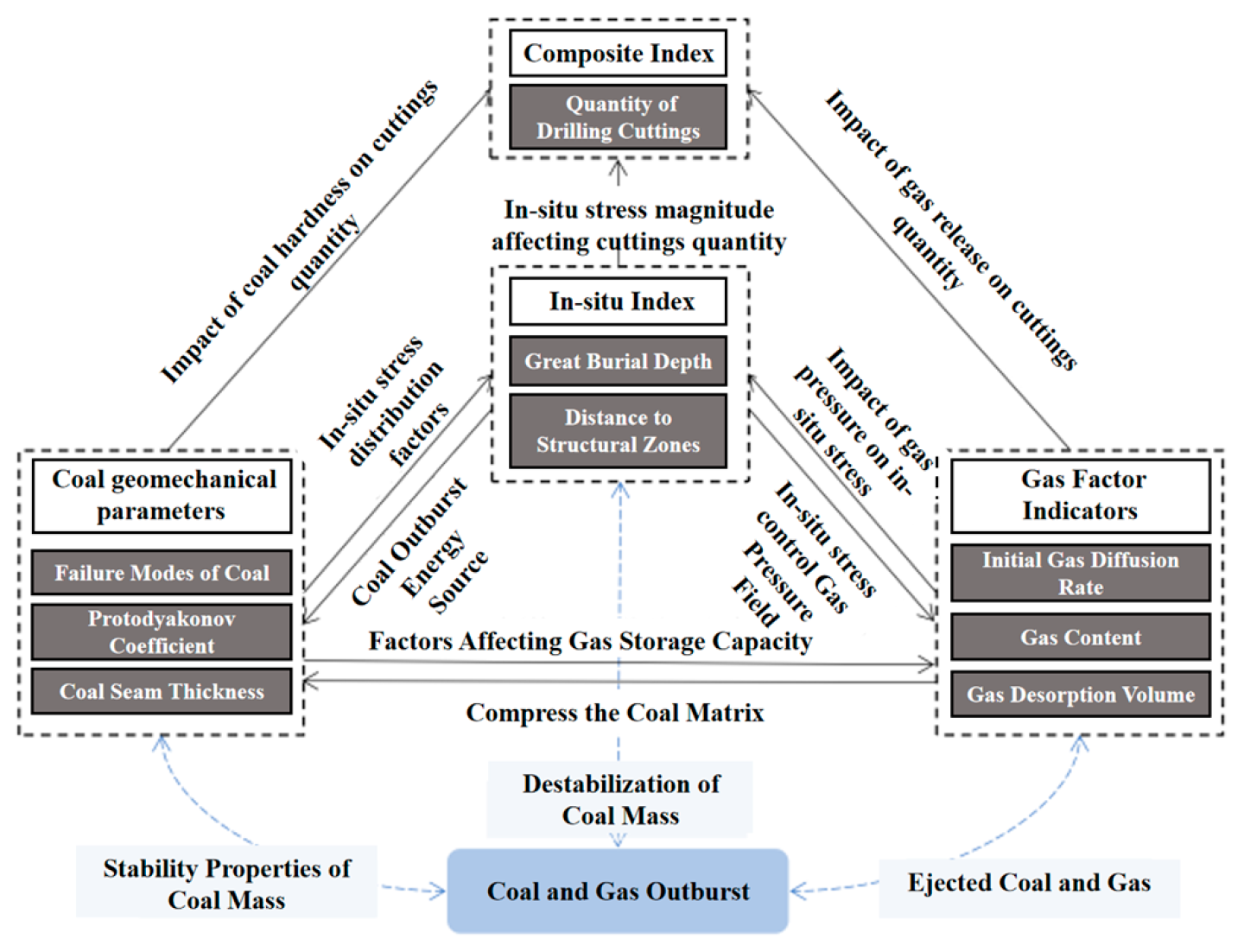
The original data contains 13 factors as the characteristic indices of coal and gas outburst prediction: coal failure type, initial gas emission speed, coal firmness coefficient, gas content, three groups of gas desorption capacity, three groups of amount of drilling cuttings, distance from the geological structural belt, buried depth, and coal thickness. The synthetic action hypothesis is combined with the coal and gas outburst index system, as shown in Figure 1:
(1)
Crustal stress. Crustal stress is a natural stress free of engineering disturbance in the earth’s crust, playing a relatively important role in coal and gas outburst. Not composed of a single stress factor, crustal stress is formed by multi-stress superposition, mainly including strata stress, concentrated stress, and tectonic stress. The buried depth mainly affects strata stress and concentrated stress. With the increase in coal seam depth, gas is further endowed with power, aggravating the risk of outburst. The distance from the geological structural belt mainly influences tectonic stress, and the division of tectonic complexity is closely related to such characteristics as faults, wrinkles, and joints [19]. In special small tectonic belts that cannot be discovered and surveyed by the existing detection techniques, this index can be quantitatively substituted by the tectonic activity of geomorphic features to reduce errors.
(2)
Gas factors. Gas refers to the methane-dominated flammable and explosive gas produced from coal seams and surrounding rocks in mining. As a necessary condition for coal and gas outburst, gas functions mainly by throwing and transporting coal masses out in the process of outburst [20]. The indices closely correlated with gas factors include the initial gas diffusion speed, gas content, and gas desorption capacity. A danger of outburst will occur when the gas content and gas diffusion speed in a coal seam reach specific critical values.
(3)
Physical and mechanical properties of coal. This factor, which also determines the difficulty in outburst occurrence and development, is related to such factors as coal failure type, coal firmness coefficient, and coal thickness [21]. The smaller the coal firmness coefficient, the softer the coal body; the greater the coal seam thickness, the poorer the coal stability. All the above factors will intensify the risk of outburst.
(4)
Comprehensive index. The amount of drilling cuttings is an index that comprehensively reflects the stress, gas pressure, and physical and mechanical properties of coal. The harder the coal body, the smaller the amount of drilling cuttings. A higher crustal stress will aggravate the difficulty in drilling, further increasing the amount of drilling cuttings.

2.2. Evaluation of Coal and Gas Outburst Risk

In this study, a multi-index comprehensive evaluation system was established based on the original data features when assessing the risk of coal and gas outburst. The specifically selected evaluation factors included the on-site drilling and spraying borehole phenomenon, amount of outburst coal body, crown drilling effect, and typical dynamic phenomenon [22]. The evaluation criteria are listed in Table 1.
According to the actual situation on the site, if no measures have been taken and no outburst has occurred, it means no risk of outburst, and the original data is expressed by 0.1; a general risk of outburst is considered if 12 to 15 groups of pressure relief holes are drilled, or with the company of the outburst of a certain amount of coal (less than 100 tons), and the original data is expressed by 0.6; and a serious risk is identified when 20 groups or more pressure relief holes are drilled, or with the company of the outburst of a large amount of coal (over 100 tons), and the original data is denoted as 1. In this study, for further analysis and processing, the risk of outburst in the original data is quantitatively given a value of 0 (0.1 in the original data means no risk of outburst), 1 (0.6 in the original data means a general risk of outburst), and 2 (1 in the original data means a serious risk of outburst).

2.3. Characteristic Engineering

2.3.1. Statistical Test of Data

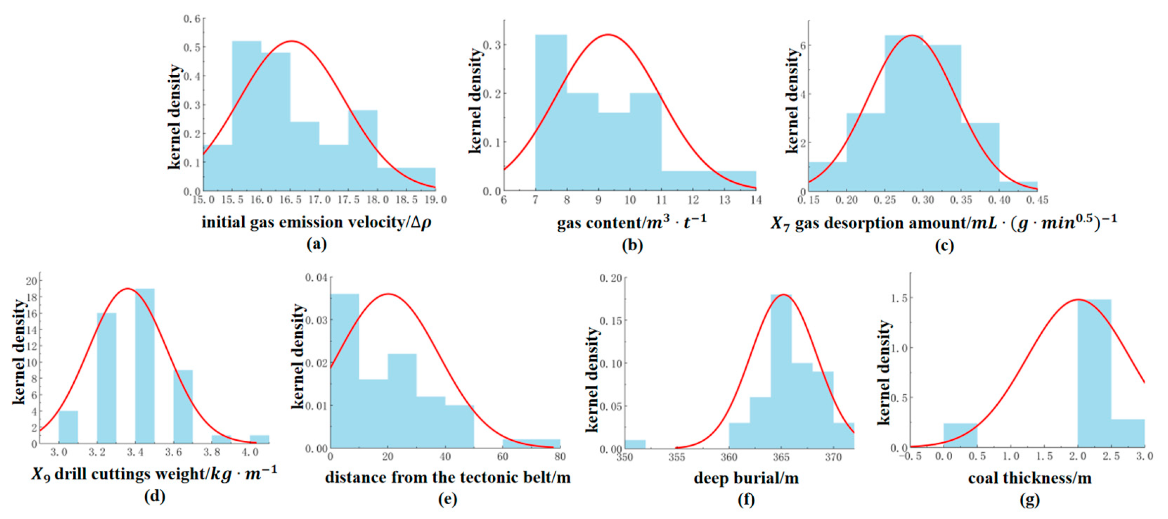
To further improve the fitting and generalization capabilities of the model and explore the inherent law of datasets, the original datasets were first subject to a descriptive statistical analysis (Table 2). The reasonability of continuous variable data was tested through a normal distribution, followed by the normally distributed curve fitting based on the least squares method. The results show that several groups of key variables present a relatively stable normal distribution trend, as shown in Figure 2.

2.3.2. Spearman Correlation Analysis

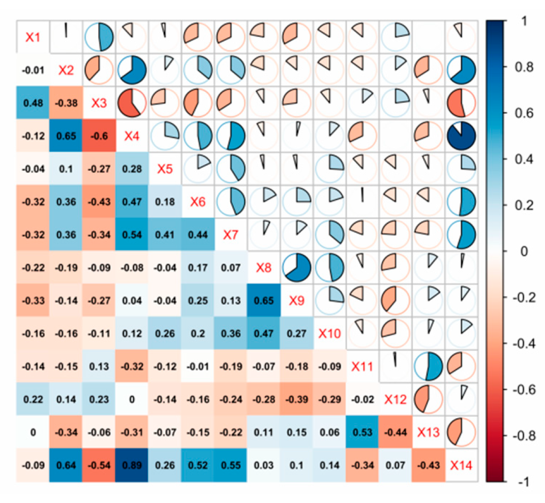
Compared with the Pearson correlation coefficient, the Spearman correlation coefficient can measure the correlation between variables in nonlinear processes more easily, along with higher robustness for related outliers, making it applicable to mining the correlation between the features of coal and gas outburst data. The results are exhibited in Figure 3:
(1)
Correlation analysis between each feature and outburst risk level: The four variables—the initial gas diffusion speed, the coal firmness coefficient, gas content, and the 2nd gas desorption capacity—are closely related to the gas outburst risk level. Among them, the correlation coefficients of X2 (initial gas diffusion speed) and X6–X7 (the second and third gas desorption capacities) with X14 (outburst risk) are 0.64, 0.52, and 0.55, respectively, reaching moderate positive correlation degrees; the correlation coefficient between X4 (gas content) and X14 (outburst risk) is 0.89, reaching a highly positive correlation degree; and the correlation coefficient between X3 (coal firmness coefficient) and X14 (outburst risk) is −0.54, reaching a moderate negative correlation degree.
(2)
Correlation analysis between feature sets: Among the feature indices regarding coal and gas outburst data, specific correlations are observed between multiple groups of variables, e.g., some moderately correlated feature sets: the correlation coefficient between X2 (initial gas diffusion speed) and X4 (gas content) is 0.65, and that between X8 (amount of drilling cuttings at the first position) and X9 (amount of drilling cuttings at the second position) is 0.65.
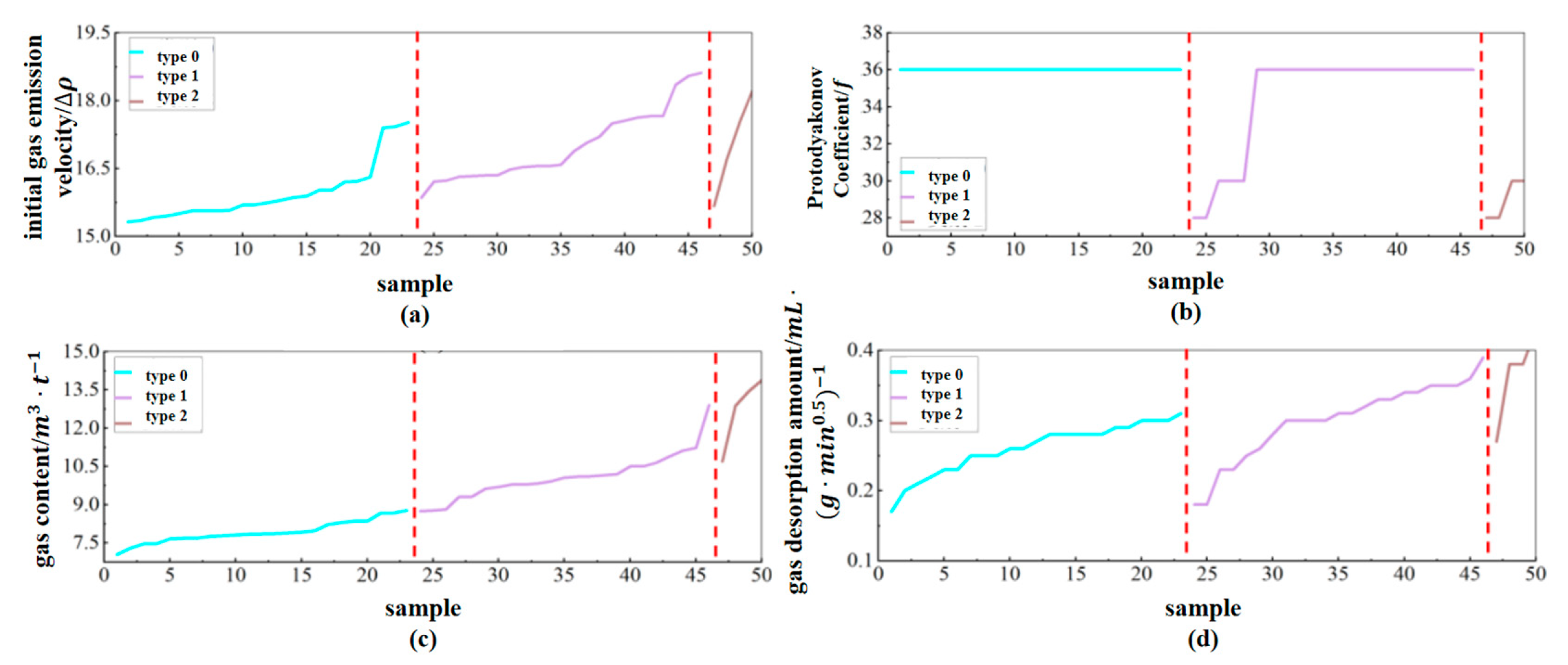
To further probe into the correlation between four significant features and outburst risk level, the initial gas diffusion speed, coal firmness coefficient, gas content, and 2nd gas desorption capacity under different outburst risk levels were subject to a visualization analysis, as shown in Figure 4. The following laws were discovered: Initial gas diffusion speed (Figure 4a): the initial gas diffusion speeds of Categories 1 and 2 are slightly higher than that of Category 0, but the difference is insignificant, indicating its minor influence on the outburst risk. Coal firmness coefficient (Figure 4b): the coal firmness coefficient of Category 0 is stabilized at 0.36, while those of Categories 1 and 2 are evidently low, meaning that the lower the firmness coefficient, the higher the outburst risk. Gas content (Figure 4c): the gas content range of Category 0 is 7.0–8.7, those of Categories 1 and 2 are 8.7–13.9, and that of Category 2 remains higher than 10.7, manifesting that gas content is an important factor affecting the outburst risk. Second gas desorption capacity (Figure 4d): the gas desorption capacities of Categories 1 and 2 are higher than that of Category 0, reflecting that the increasing desorption capacity will markedly increase the outburst risk.

2.3.3. Contribution Rate Analysis of Influencing Factors Based on RF

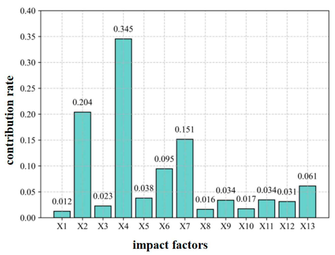
The correlation between data features and their redundancy will directly impact the modeling difficulty and training accuracy. To reduce the correlation between data attributes, the outburst-affecting factors were subject to ranking and dimension reduction through the RF method in the aspect of contribution rate [23]. As shown in Figure 5, X2, X4, and X7 reach the highest contribution rates, all of which are above 0.15, corresponding to three significant variables—initial gas diffusion speed, gas content, and 3rd gas desorption capacity, respectively; X1, X8, and X10 have relatively low contribution rates, all of which are about 0.01. Considering their weak influence on the outburst prediction result, the three variables were excluded during modeling, aiming to reduce data redundancy.

3. Establishment of the Coal and Gas Outburst Early Warning Model

3.1. Processing of Unbalanced Data Based on Borderline-SMOTE

Borderline Synthetic Minority Oversampling Technique (Borderline-SMOTE), a technique of processing unbalanced data, improves the traditional SMOTE in terms of fuzzy category boundaries and minority category distribution by introducing the division strategy for neighboring minority samples. The core idea of this technique is to take the number of majority category samples included in the k-nearest neighbor of minority category samples as the judgment condition for boundary samples and to expand the minority categories of boundary samples.
(1)
Samples nearest to the minority category sample are solved through the k-nearest neighbor method, and their distance is solved as per Formula (1): solving the difficulty in learning boundary samples in the process of expanding unbalanced data [24], specifically as follows:
d ( X , Y ) = i = 1 n ( x i y i ) 2 .
where d ( X , Y ) denotes the Euclidean distance between two sample points, X i and X j are two sample points (feature vectors) in the dataset, n is the number of feature dimensions, and X i and X j are the k-th feature values of the two samples, X = ( x i , x 2 , , x n ) and Y = ( y 1 , y 2 , , y n ) .
(2)
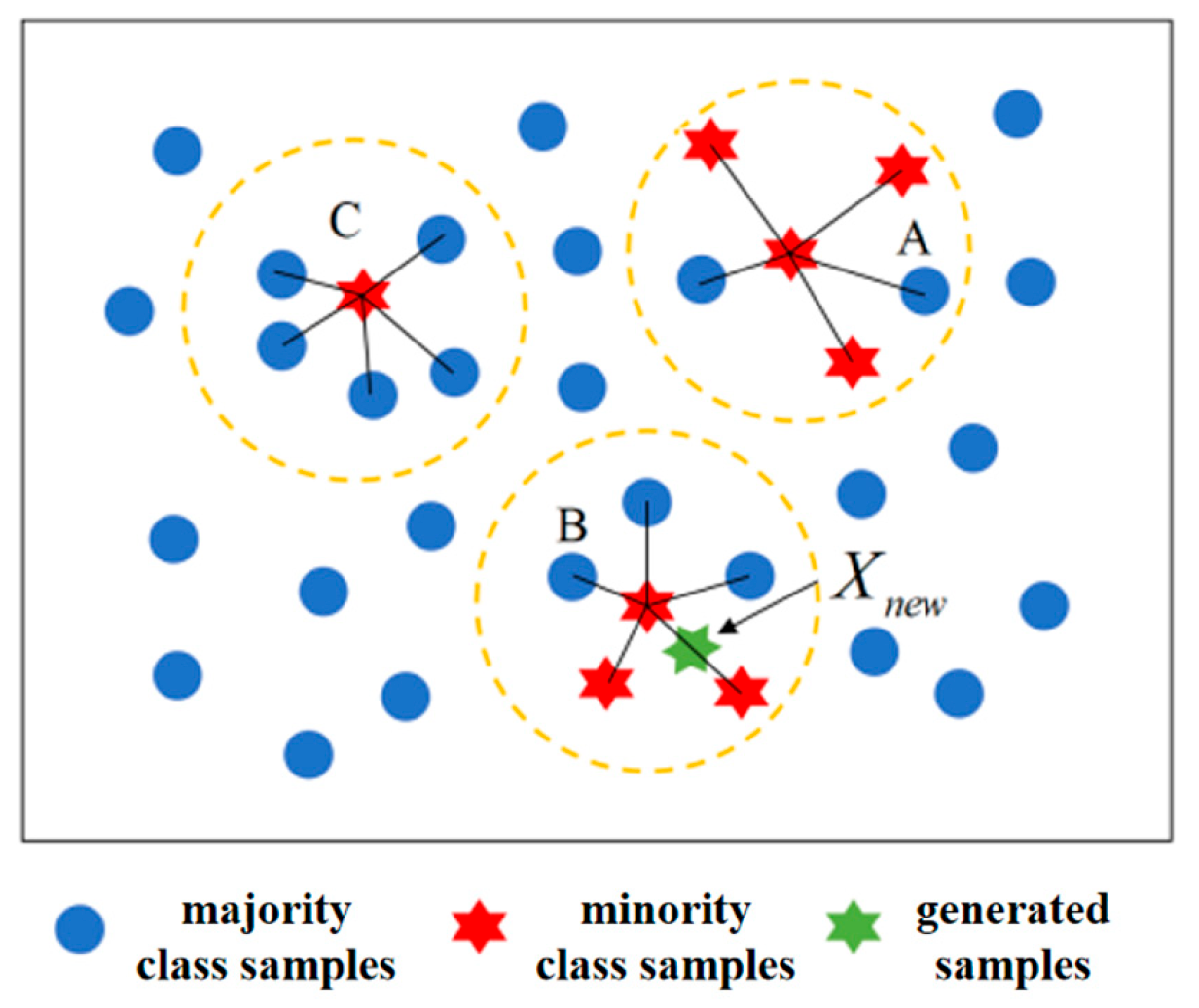
The category samples in the k -nearest neighbor samples are counted and denoted as n . Category division is performed for this minority category sample according to the rules corresponding to different n values. If 0 n k , this sample is considered a safety point when over half of the points around the sample are minority category samples, as shown in Point A in Figure 6; if k / 2 n k , this sample is regarded as a risk point when over half of the points around the sample are majority category samples, e.g., Point B in Figure 6; and if n = k , this sample is considered a noise point when all points around the sample are majority category samples, like Point C in Figure 6.
(3)
Since risk categories can be easily misclassified, only the randomly selected minority category samples marked as risk categories were subject to the synthesis of new samples, as seen in Formula (2):
X n e w = X i + δ × ( X ^ i X i ) .
where X i denotes a randomly selected minority-class sample that has been labeled as a risk point (i.e., more than half of its k-nearest neighbors belong to the majority class); X i j denotes one of the risk-point samples among the k-nearest neighbors of X i ; and rand(0,1) is a random number drawn from a uniform distribution over the interval [0, 1], which determines the interpolation position between X i and X i j . The newly synthesized sample X n e w is assigned the same class label as X i (minority class). This interpolation procedure generates new samples along the line segment connecting the selected minority sample and its neighboring risk-point sample, thereby augmenting the minority class while preserving the local data structure. The complete synthesis process is governed by Equation (2).
The Borderline-SMOTE algorithm has been proven effective in other imbalanced geohazard datasets, such as landslide susceptibility mapping [25].

3.2. Coal and Gas Outburst Model Based on Stacking Ensemble Learning

3.2.1. Principle of Stacking Ensemble Learning

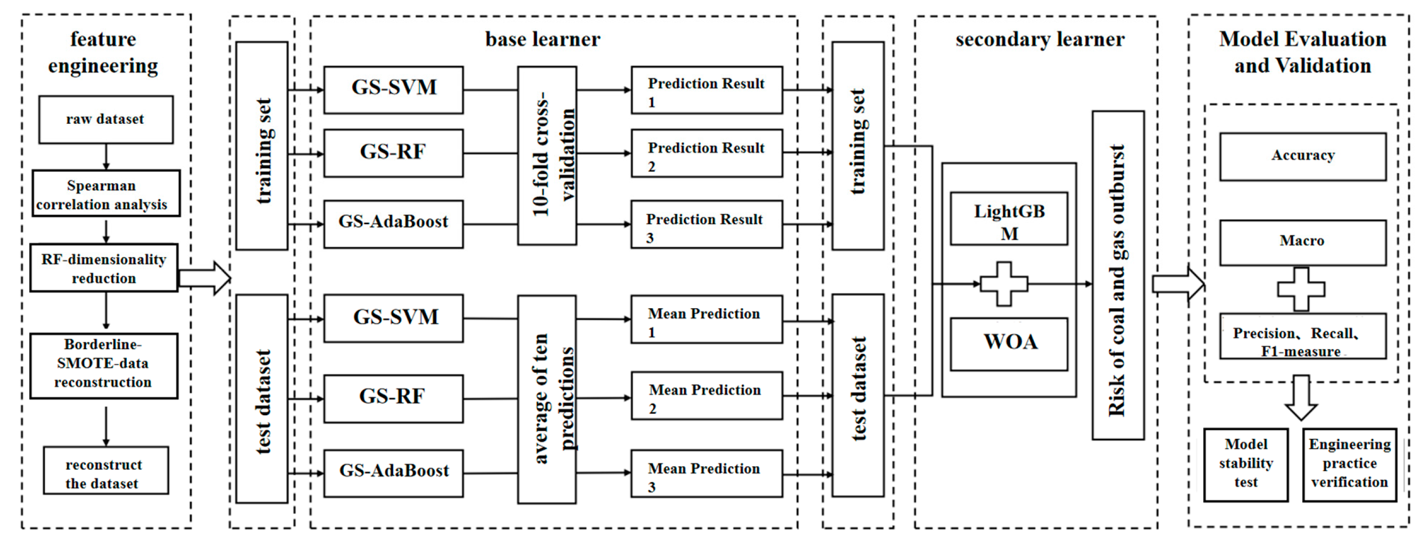
Ensemble learning refers to combining multiple weak learners in a specific manner, constructing a strong learner with better performance than a single learner. Ensemble learning methods include Bagging, Boosting, and Stacking. The former two adopt a linear ensemble strategy and combine homogeneous weak learners according to a deterministic algorithm to form a strong learner. Different from Bagging and Boosting, Stacking utilizes a nonlinear ensemble strategy and establishes a multi-layer strong learner by combining heterogeneous learners, where the top-layer learner can further enhance the generalization capability of the model through the output result of the lower-layer learner [26]. The Stacking model integrates the merits of a simple structure, high performance, and strong classification ability, obeying the following core idea: first, the training set is subject to learning training through a primary learner, and then the result of the primary learner is taken as the input of the secondary learner for training to acquire the final prediction result. The algorithm flow of Stacking ensemble learning is displayed as follows.
Step 0: Algorithm input and output
Input: X train n × d , y train n , X test m × d , M base learners, M meta meta-learner, and K-fold cross-validation
Output: Final prediction result y pred m of the test set
Step 1: Folds splitting of cross-validation
f o l d s K F o l d S p l i t X train , y train , K .
Step 2: The base learner is trained, and the prediction of the training set and test set is generated.
First, the prediction matrix H train n × M for the training set and the prediction matrix H test m × M for the test set are initialized.
For i = 1 to M base learners, their prediction values y ^ train ( i ) 0 n  and  y ^ t e s t ( i ) 0 m on the training set and test set are respectively initialized.
In the i = 1 to K-fold cross-validation for the i-th base learner, the training set and validation set numbers of the present fold are acquired:
( X tr , y tr ) , ( X val , y val ) folds [ k ] .
The i-th base learner is trained:
f i , k T base ( X tr , y tr , BaseModel i ) .
The prediction y ^ val ( i , k ) f i , k ( X val ) , is performed on the validation set, and the prediction result is recorded into the prediction matrix of the training set:
y ^ train ( i ) [ val _ indices ] y ^ val ( i , k ) .
The prediction y ^ test ( i , k ) f i , k ( X test ) , is performed on the test set, and the prediction results of each fold are averaged:
y ^ test ( i ) y ^ test ( i ) + 1 K y ^ test ( i , k ) .
After cross-validation, the prediction result H train [ : , i ] y ^ train ( i ) of the i-th base learner on the training set and the prediction result of H test [ : , i ] y ^ test ( i ) on the test set are saved in the matrix.
Step 3: The meta-learner is trained.
Step 4:
g meta T meta ( H train , y train , MetaModel ) .
The final prediction result is generated.
y pred g meta ( H test ) .

3.2.2. Modeling

Three classification learners—SVM, AdaBoost, and RF—were selected as the first-layer primary learners in the Stacking ensemble learning framework. The parameters of the primary classifier model were optimized through the grid search (GS) method. The LightGBM model was chosen at the second layer, and the important model parameters—max_depth (maximum decision tree depth), feature_fraction (fraction of feature sampling), and learning_rate—were optimized using WOA, aiming to enhance the model accuracy and generalization capability. In addition, the classification performance of each classifier was tested by means of ten-fold cross-validation. The overall framework of the established coal and gas outburst risk prediction model based on the Stacking ensemble learning theory is displayed in Figure 7.

4. Experimental Results and Discussion

4.1. Model Evaluation Indices

The model was evaluated using the following criteria: accuracy, precision, recall, and F1-score. Accuracy refers to the ratio of the number of all samples with correctly predicted categories to the total number of samples, reflecting the overall classification performance of the model; considering the category imbalance of original data, the precision, recall, and F1-score were calculated through macro-averaging, which can further concern the prediction performance of the model on unbalanced subcategories; recall denotes the ratio of the number of samples correctly classified under the outburst risk level of 3 to the number of samples belonging to this category; and F1-score denotes the harmonic mean of accuracy and recall, reflecting the overall classification performance of the model. Here, T P i , F P i , F N i , and T N i denote the numbers of true positives, false positives, false negatives, and true negatives for the i-th category, respectively.
M a c r o _ r e c a l l = 1 n i = 1 n T P i T P i + F N i .
M a c r o _ F 1 = 2 P × R P + R .
where n is the total number of sample categories; T P i stands for the number of samples correctly predicted as Category i ; T N i is the number for samples mistakenly predicted as Category i ; F P i is the number of samples that belong to other categories while mistakenly predicted as Category i ; F N i is the number of Category i samples mistakenly predicted as other categories; P is the precision under macro-averaging calculation; and R denotes the recall under macro-averaging calculation.

4.2. Data Balancing Effect

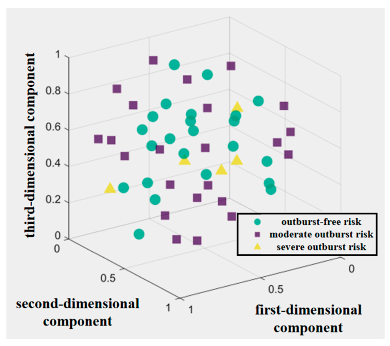
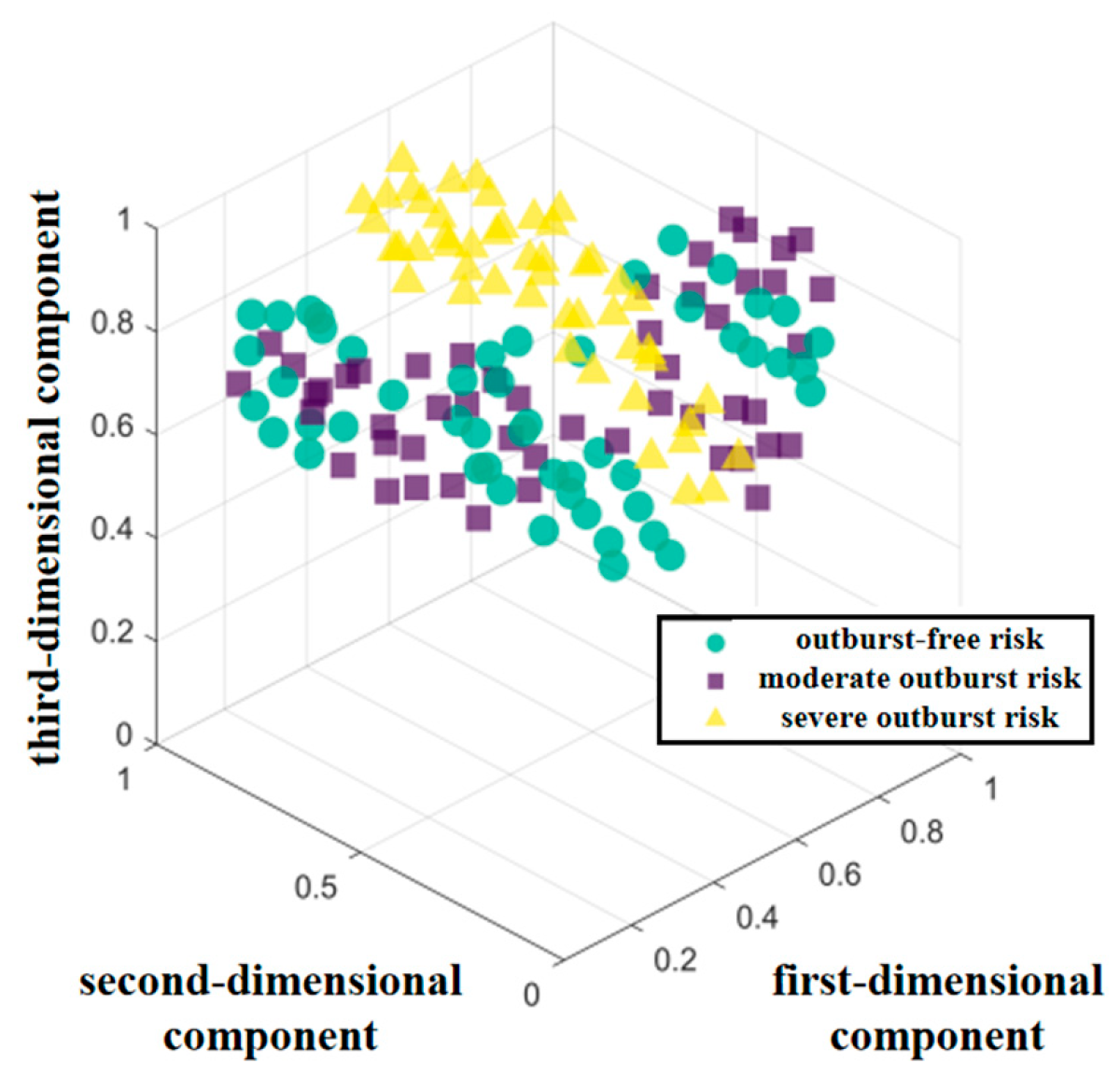
In this study, the total number of original samples was 50, where the samples that belong to Category 2 (serious outburst risk) only accounted for 4/50, and the data distribution was extremely unbalanced, significantly affecting the performance of the classifier. To improve the imbalance of coal and gas outburst data, the data samples were expanded using Borderline-SMOTE to achieve data enhancement. Given the small number of Category 2 samples (only 4), the model parameter was set to k_neighbors = 4. By expanding samples of various categories, 50 samples of Categories 0, 1, and 2 were respectively acquired, which effectively improved the imbalance of sample categories while enhancing their diversity.
To intuitively display the data distributions before and after balancing, the original coal and gas outburst datasets and the processed datasets were mapped into a three-dimensional space through the TSNE method. The results are displayed in Figure 8 and Figure 9, respectively. It can be observed from Figure 9 that the processed data are aggregated more tightly, and their separability is significantly enhanced compared with the discrete distribution of original data.
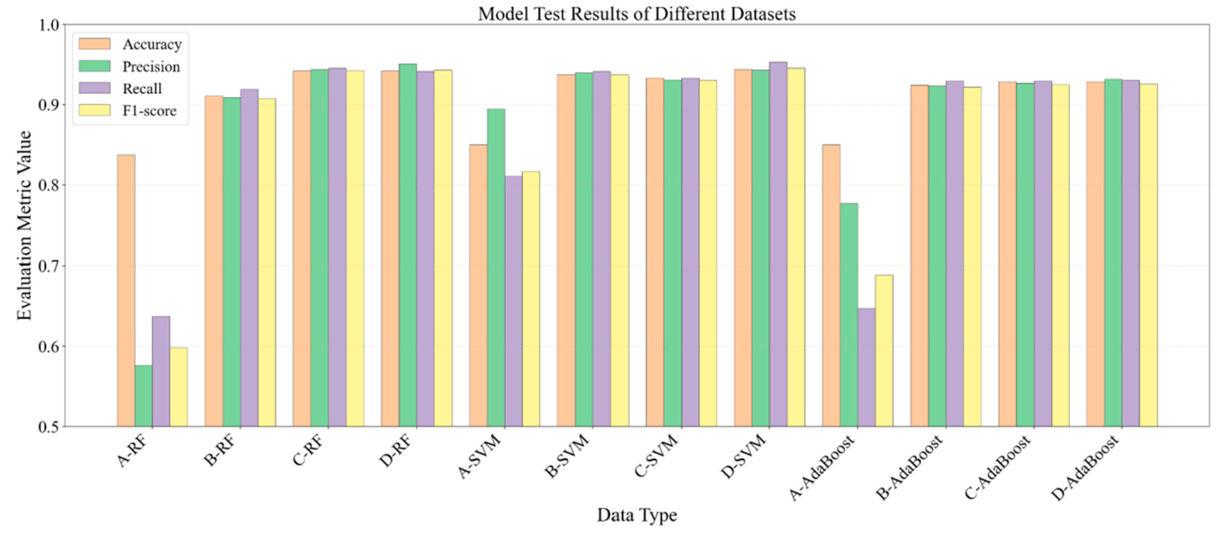
To evaluate the effectiveness of expanded data, a training test was performed on the original dataset, SMOTE expanded dataset, SMOTE-NC expanded dataset, and Borderline-SMOTE expanded dataset through the RF, AdaBoost, and SVM models. Among them, the maximum depth of RF model trees was set to 6, and the number of base classifiers was 100; the penalty factor of the SVM model was 10, and the kernel function was linear; and the maximum depth of AdaBoost model trees was 2, and the learning rate was 0.01. Each dataset was divided by a ratio of 7:3, where 70% constituted the training set and 30% formed the test set, and the mean value of each model on the test set after five tests was taken as the prediction result. Under the same parameter settings, the model performance was affected differently by different datasets. The RF, SVM, and AdaBoost models performed best on the dataset subject to RF-based dimension reduction and Borderline-SMOTE-based reconstruction. The results are listed in Table 3 and Figure 10. For clarity, the four dataset variants used in this comparison are designated as follows: A = original dataset; B = RF-SMOTE processed2; C = RF-SMOTE-NC processed; and D = RF-Borderline-SMOTE processed.
RF model: on the RF-Borderline-SMOTE dataset, the accuracy, precision, recall, and F1-score increased by 12.5%, 65.0%, 47.7%, and 57.5%, respectively, compared with those on the original dataset. SVM model: on the RF-Borderline-SMOTE dataset, the four indices grew by 11.1%, 5.4%, 17.5%, and 15.7%, respectively, compared with those on the original dataset, accompanied by minor improvements in comparison with those on the RF-SMOTE and RF-SMOTE-NC datasets. AdaBoost model: on the RF-Borderline-SMOTE dataset, the four indices increased by 9.2%, 19.9%, 43.7%, and 34.4%, respectively, relative to those on the original dataset.
The results reveal that RF-based dimension reduction in combination with Borderline-SMOTE effectively relieves data imbalance and redundancy, markedly improving the model’s prediction performance.

4.3. Parameter Optimization and Model Validation

4.3.1. Model Training and Parameter Optimization

First, the dataset processed by RF-Borderline-SMOTE was standardized and randomly divided into a training set (70%) and a test set (30%). The RF, SVM, and AdaBoost models of the primary classifiers were separately trained, and their performance on the Borderline-SMOTE reconstructed dataset was verified through ten-fold cross-validation. Then, the model parameters were adjusted through the GS method, and the optimal parameters of the base models are exhibited in the following Table 4.
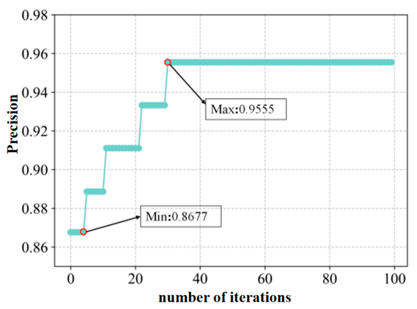
During the parameter optimization of the LightGBM model, the three key parameters—max_depth, feature_fraction, and learning_rate—of this model were optimized through WOA with the accuracy of the test set as the objective function: the optimization range for max_depth was [6, 20]; feature_fraction represents the fraction of feature sampling, with an optimization range of [0.001, 1]; and learning_rate indicates the updated step length in the control weight, with an optimization range of [0.001, 1]. The parameter settings for WOA were as follows: pop (population size) = 50, MaxIter (maximum number of iterations) = 100, dim = 3, lb = [6, 0.001, 0.001], and ub = [20, 1, 1]. The final optimization result achieved the best accuracy of 0.9555 upon the 29th iteration, and the optimization iteration curve is displayed in Figure 11. Finally, max_depth, feature_fraction (the fraction of features randomly sampled for each tree, ranging from 0.001 to 1, where 1 means all features are used), and learning_rate of the LightGBM model are 7, 0.2, and 0.1, respectively.

4.3.2. Comparative Evaluation of Models

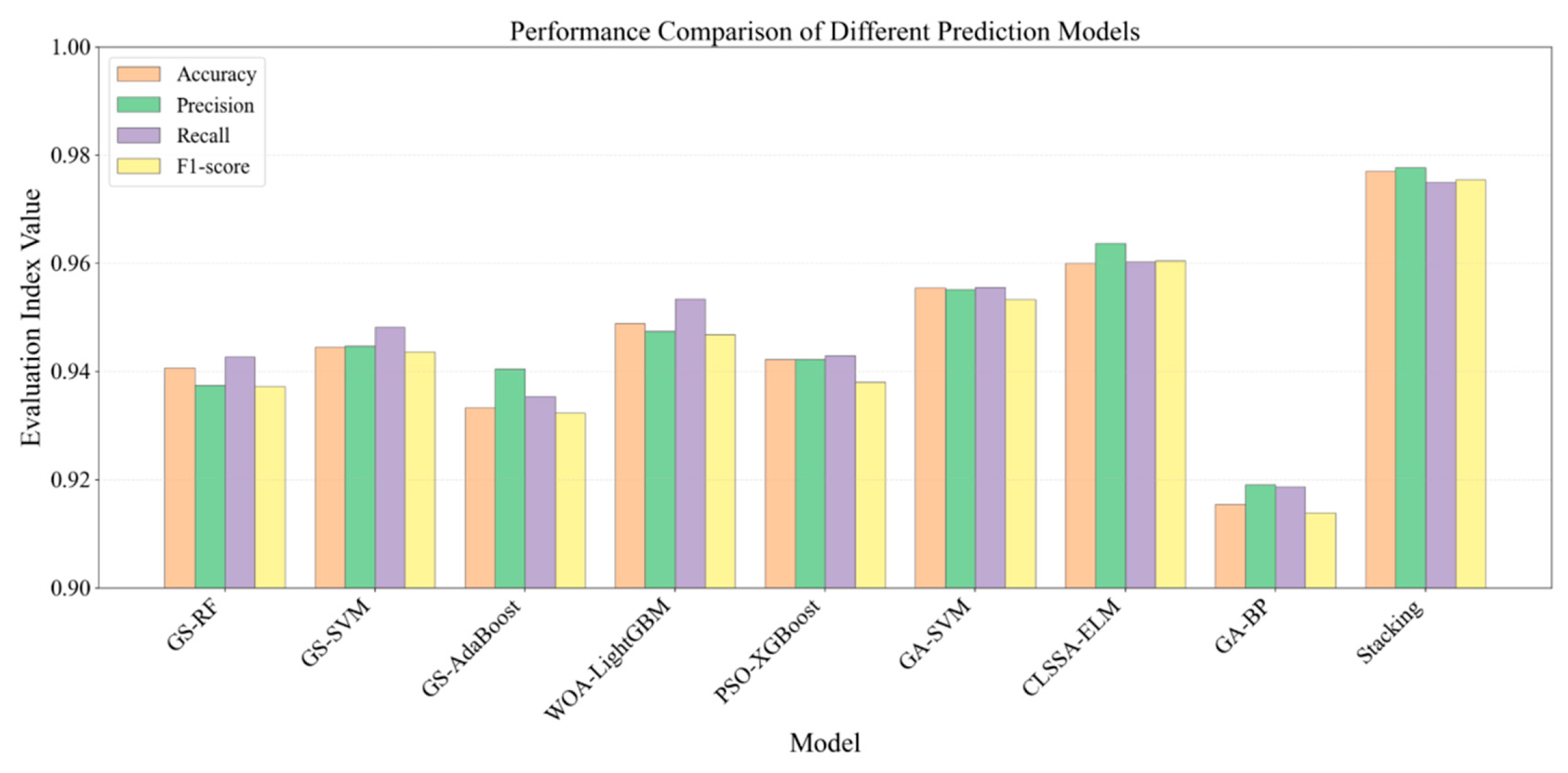
To verify the accuracy of the Stacking ensemble model, the dataset expanded by RF-Borderline-SMOTE was taken as the model test dataset. The prediction results obtained by single models, the common coal and gas outburst prediction models, and the Stacking ensemble model were comparatively analyzed, involving such models as CLSSA-ELM, GA-SVM, and GA-BP. Among them, the hidden-layer nerve cell of CLSSA-ELM was set to (100, 100), with ReLU serving as the activation function; the penalty factor of GA-SVM was 0.01, and a polynomial kernel function with an order number of 8 was chosen; for PSO-XGBoost, the maximum tree depth, learning rate, and number of base learners were 3, 0.1, and 100, respectively; and the hidden-layer structure of GA-BP was (150, 100), ReLU was selected as the activation function, the Adam optimizer was used, and the initial learning rate was 0.001. The dataset was divided into a training set (70%) and a test set (30%), a cross-validation was performed, and the mean value of each model index on the test set after ten predictions was selected as the final result. The test results of each model are displayed in Table 5 and Figure 12.
Through the comparative analysis in Table 5, the Stacking model achieves significant improvements in all four indices compared with GS-optimized single models, achieving an increase of 3.86%, 4.30%, 3.43%, and 4.09% in accuracy, precision, recall, and F1-score, respectively, relative to GS-RF; 3.44%, 3.49%, 2.83%, and 3.38%, respectively, relative to GS-SVM; and 4.68%, 3.96%, 4.23%, and 4.63%, respectively, relative to GS-AdaBoost. Similarly, the Stacking model markedly reduces the classification error rate of each category, where the error rates for Categories 1, 0, and 2 respectively decline by 93.73%, 89.39%, and 66.27% compared with the maximum values in single models, exhibiting higher prediction accuracy and generalization capability. Additionally, compared with the LightGBM model under WOA, the Stacking model achieves an increase in the four indices by 2.96%, 3.10%, 2.27%, and 3.03%, respectively. In comparison with other models like CLSSA-ELM, the Stacking model gains 1.77%, 1.45%, 1.53%, and 1.56% increases in accuracy, precision, recall, and F1-score, respectively, and meanwhile, the classification error rates for different categories are more evenly distributed and relatively low on the whole. To sum up, the Stacking model performs excellently in the comparative test of different categories, and its marked performance improvement and stronger generalization capability further evidence its effectiveness and stability in the gas outburst risk prediction.

4.4. Model Stability Test

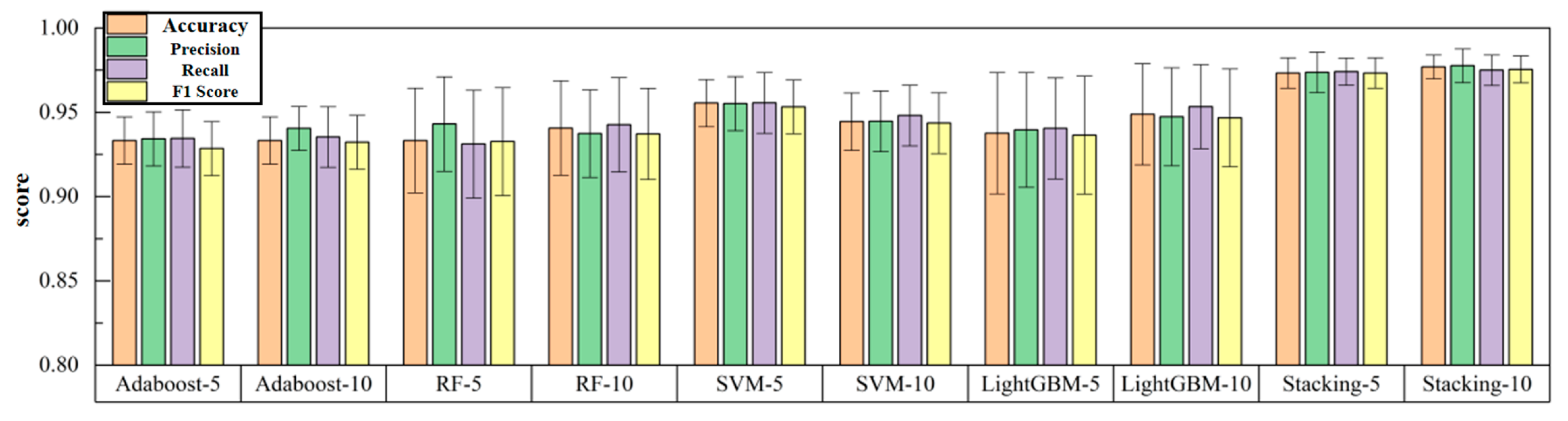
To further test the stability of the Stacking model, the variation trends of the four indices of the Stacking model and base models under 5 and 10 tests were compared, specifically as shown in Figure 13. Under the different calculation methods for averaging the 5 test results and 10 test results, the variations in the four indices of the Stacking model are evidently smaller than those of other single models under other structures, indicating its high robustness. Compared with the other test models, the Stacking model achieves a stronger generalization capability on the coal and gas outburst dataset after Borderline-SMOTE reconstruction and RF feature extraction, accompanied by a higher stability and prediction accuracy. This further proves that the established Stacking model can serve as an effective method for the coal and gas outburst risk prediction.

5. Analysis of Coal and Gas Outburst Cases

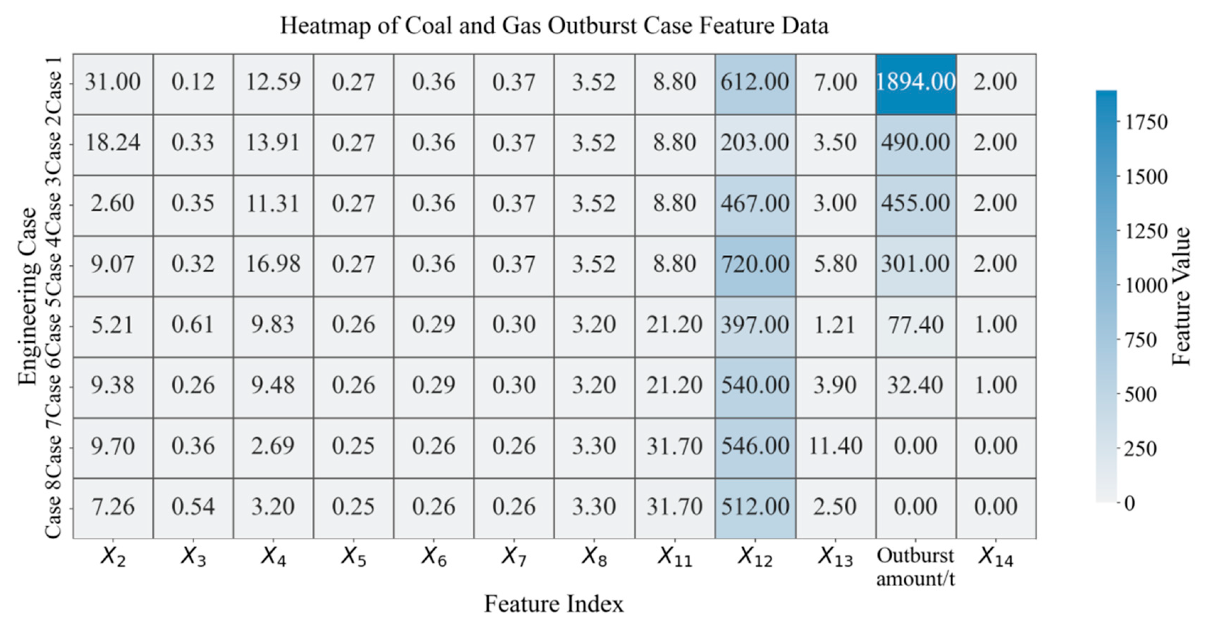
Eight practical coal and gas outburst cases [27,28] were selected to verify the established outburst risk prediction model, and the parameters of each case are listed in Table 6 and Figure 14. Given the difference in index selection in practical research, three indices—gas desorption capacity, amount of drilling cuttings, and distance from the geological structural belt—were missing in the eight cases. According to the risk level corresponding to the actual outburst amount, data errors were further reduced by substituting with the mean value of the category index with the risk level corresponding to the original dataset. The relevant backgrounds of the coal and gas outburst cases were: the rock tunneling working face of 21# track dip roadway of Henan Daping Coal Mine on 20 October 2004 (Case 1); driving working face of 1132 transportation roadway in Hexi mining area of Guizhou Xiangshui Coal Mine on 24 November 2012 (Case 2); driving working face of 4112 transportation roadway of Songshu Town Coal Mine +100 m east 1# mining area in Jilin on 6 March 2016 (Case 3); 15-47-11111 fully mechanized coal mining face of Pingdingshan 13th Mine in Henan on 6 September 2016 (Case 4); and historical coal and gas outburst data of Qianjiaying Mine of Kailuan Group (Cases 5–8).
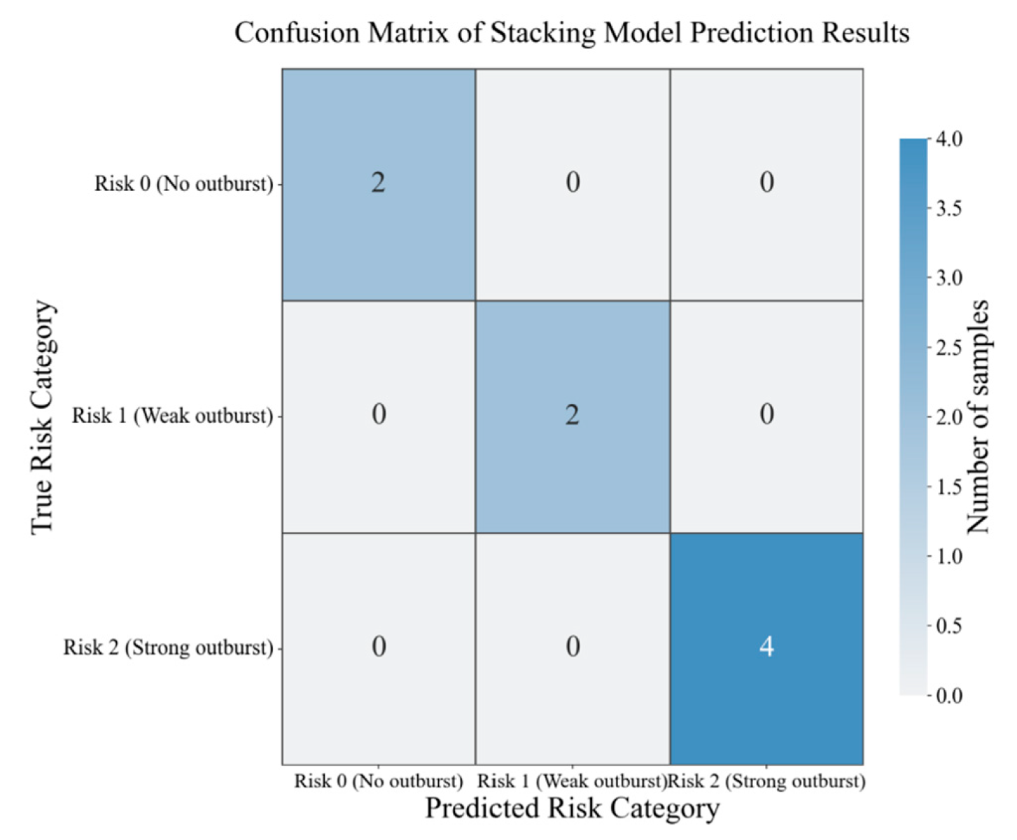
After the data of coal and gas outburst cases were standardized according to the same parameters as the original data, the data were input into the test model to obtain the final prediction results (Table 7 and Figure 15). The results show that the GA-BP model performs poorly in the prediction of Category 1 samples, with an overall accuracy of 62.5%; the CLSSA-ELM model has poor performance in the prediction of case data, with the accuracy only reaching 50%. Comparatively, the Stacking model established in this study realizes the accurate recognition of all eight coal and gas outburst cases, indicating its significant advantages in the identification of outburst risks.

6. Conclusions

In this study, a coal and gas outburst risk prediction model based on Stacking ensemble learning was put forward, and the factors influencing coal and gas outburst were mined by combining characteristic engineering. Finally, the following conclusions were mainly drawn:
(1)
When mining the influencing factors of coal and gas outburst, the coal and gas outburst datasets were subject to the Spearman correlation analysis. Combining the coal and gas outburst index system and the visualization analysis and test, the relevant conclusions were drawn as follows: The initial gas diffusion speed, gas content, and gas desorption capacity have positive effects on the outburst risk; the threshold interval for the gas content without any gas outburst risk is 7.0–8.7 and that for the gas content with gas outburst risks is 8.7–13.9. The coal firmness coefficient influences the outburst risk negatively: the lower the coal firmness coefficient, the higher the corresponding outburst risk.
(2)
In the characteristic engineering processing of data, the contribution rates of characteristic factors were ranked through the RF method, and redundant variables were excluded; the dataset after RF-based dimension reduction was reconstructed via the Borderline-SMOTE algorithm, improving the sample data imbalance of the original data, further enhancing data diversity and category balance, and ensuring a reasonable data distribution.
(3)
The Stacking ensemble learning model established in this study reaches 0.9770, 0.9777, 0.9750, and 0.9755, respectively, in accuracy, precision, recall, and F1-score, with 2.96%, 3.10%, 2.27%, and 3.03% increases compared with those of the WOA-LightGBM model, which performs well among single models. In comparison with such models as CLSSA-ELM and PSO-XGBoost, the Stacking model performs best in prediction accuracy, error control, and stability, and the classification error rates for each category are distributed in the most balanced manner. In the prediction of practical engineering cases, the Stacking model exhibits relatively higher accuracy and applicability in the prediction of coal and gas outburst risks, manifesting that the proposed Stacking model effectively fuses the advantages of characteristic engineering and ensemble learning, providing reliable technical support for the prediction of coal and gas outburst risks.

7. Outlook and Limitations

Despite its superior performance, the Stacking ensemble model has inherent limitations. First, the training and inference costs are substantially higher than those of single models due to the multi-learner architecture and K-fold cross-validation, which may hinder deployment in resource-constrained underground environments. Second, the base learners (RF, SVM, AdaBoost) each possess specific sensitivities—RF may overfit small datasets, SVM is vulnerable to boundary noise, and AdaBoost is susceptible to outliers—and these weaknesses may propagate through the ensemble [29]. Third, the WOA optimization, while effective, introduces stochastic variability and computational overhead without guaranteeing global optimality [30]. Fourth, the model relies on the complete set of 13 input indicators; missing field data would compromise prediction reliability. Finally, the leaf-wise growth strategy of LightGBM poses a potential overfitting risk when applied to limited samples.
For future work, the following directions are recommended:
(1)
expanding the dataset by collecting outburst records from multiple coal mines with diverse geological settings to enhance model generalizability;
(2)
exploring lightweight ensemble strategies or model compression techniques to reduce inference time for on-site applications [31];
(3)
incorporating interpretability tools such as SHAP or LIME to provide actionable insights for mine safety engineers [32];
(4)
investigating the integration of real-time monitoring data (e.g., acoustic emission or electromagnetic radiation signals) into the current framework to enable dynamic early warning [33].

Author Contributions

Conceptualization, Y.L., X.Q., Y.G. and J.C.; data curation, Y.L., X.Q., K.C. and S.Y.; formal analysis, K.C., S.Y. and R.C.; funding acquisition, Y.G. and J.C.; investigation, Y.L., K.C. and R.C.; visualization, S.Y. and R.C.; writing—original draft, Y.L. and X.Q.; writing—review and editing, Y.G., R.C. and J.C. All authors have read and agreed to the published version of the manuscript.

Funding

This study was supported by the Hebei Provincial Natural Science Foundation (Grant No. E2024209077) and the National Natural Science Foundation of China (Grant Nos. 52504219, 52304216).

Data Availability Statement

The data that support the findings of this study are available from the corresponding author upon reasonable request.

Conflicts of Interest

Author Kai Cui was employed by the company Hebei Lvzhi Xinglan Environmental Technology Co., Ltd. The remaining authors declare that the research was conducted in the absence of any commercial or financial relationships that could be construed as a potential conflict of interest.

Abbreviations

The following abbreviations are used in this manuscript:
WOAWhale optimization algorithm
GSGrid search
AEAutoencoder
IPSOImproved particle swarm optimization
KELMKernel extreme learning machine
CLSSAChaotic lens slime swarm algorithm
BPBack propagation
SMOTESynthetic minority oversampling technique
KNNK-nearest neighbors
t-SNEt-distributed stochastic neighbor embedding
SMOTE-NCSMOTE for nominal continuous
ReLURectified linear unit
AdamAdaptive moment estimation
PSOParticle swarm optimization
XGBoostExtreme gradient boosting
GAResearch Hypotheses 1 to 5
SHAPSHapley Additive exPlanations
LIMELocal interpretable model-agnostic explanations

References

  1. Li, Q.C.; Wang, H.P.; Yuan, L. Experimental Study on Damage Deterioration of Coal Rock Mechanical Properties by Adsorbed Gas Volume. J. China Univ. Min. Technol. 2019, 48, 955–965. [Google Scholar] [CrossRef]
  2. Liu, T.; Lin, B. Time-Dependent Dynamic Diffusion Processes in Coal: Model Development and Analysis. Int. J. Heat Mass Transf. 2019, 134, 1–9. [Google Scholar] [CrossRef]
  3. Li, X.; Chai, Y. Determination of Pillar Width to Improve Mining Safety in a Deep Burst-Prone Coal Mine. Saf. Sci. 2019, 113, 244–256. [Google Scholar] [CrossRef]
  4. He, Z.; Wu, Q.; Wen, L.; Fu, G. A Process Mining Approach to Improve Emergency Rescue Processes of Fatal Gas Explosion Accidents in Chinese Coal Mines. Saf. Sci. 2019, 111, 154–166. [Google Scholar] [CrossRef]
  5. Zou, Q.; Liu, H.; Zhang, Y.; Li, Q.; Fu, J.; Hu, Q. Rationality Evaluation of Production Deployment of Outburst-Prone Coal Mines: A Case Study of Nantong Coal Mine in Chongqing, China. Saf. Sci. 2020, 122, 104515. [Google Scholar] [CrossRef]
  6. Cheng, X.; Chen, X.Z. Application of Grey Correlation Degree Analysis Method in Coal and Gas Protrusion Simulation Test. Coal Technol. 2018, 37, 179–181. [Google Scholar] [CrossRef]
  7. Bi, J.; Li, X.J. Analysis of Causes of Coal and Gas Protrusion Accidents Based on Fuzzy Fault Tree. Min. Technol. 2019, 19, 97–100. [Google Scholar] [CrossRef]
  8. Cheng, Y.P.; Zhou, H.X. Progress of Research on Sensitive Indicators and Their Critical Values for Coal and Gas Protrusion Prediction. Coal Sci. Technol. 2021, 49, 146–154. [Google Scholar] [CrossRef]
  9. Li, X.; Jiang, Q.; Yuan, Q. Research and Application of Early Warning System for Coal and Gas Protrusion at Working Face. Coal Eng. 2021, 53, 107–111. [Google Scholar]
  10. Wang, Y.H.; Liu, L.L.; Fu, H.; Xu, Y. Gas Protrusion Prediction Based on Acoustic Emission Multiparameter Time Series. China J. Saf. Sci. Technol. 2018, 28, 129–134. [Google Scholar] [CrossRef]
  11. Wang, E.Y.; Li, Z.H.; Li, D.X.; Liu, X.; Li, J. Application of Electromagnetic Radiation Monitoring Technology Equipment in Monitoring and Early Warning of Coal and Gas Protrusion. Coal Mine Saf. 2020, 51, 46–51. [Google Scholar] [CrossRef]
  12. Yin, L.; Wu, S.Y.; Sun, W.; Qu, H. GIS-Based Prediction of Coal Seam Gas Protrusion Hazardous Areas. Min. Res. Dev. 2021, 41, 44–49. [Google Scholar]
  13. Wu, Y.Q.; Li, H.J.; Xu, D.N. Coal and Gas Protrusion Prediction Algorithm Based on IPSO-Powell Optimised SVM. Ind. Min. Autom. 2020, 46, 46–53. [Google Scholar] [CrossRef]
  14. Xie, G.N.; Huang, R.L.; Liu, M.; Tu, N.W. L-Isomap-KELM Model for Coal and Gas Herniation. Control Eng. 2020, 27, 1802–1806. [Google Scholar]
  15. Wen, T.X.; Gao, Q. Coal and Gas Protrusion Hazard Prediction Model Based on AE-CLSSA-ELM. China Saf. Prod. Sci. Technol. 2023, 19, 73–79. [Google Scholar]
  16. Long, N.Z.; Yuan, M.; Ao, X.J.; Li, X.; Zhang, P. Coal and Gas Protrusion Intensity Prediction Based on LLE-FOA-BP Model. Ind. Min. Autom. 2019, 45, 68–73. [Google Scholar]
  17. Yan, X.; Zhu, Y.H.; Tu, N.W.; Wu, S.; Wang, Y. Prediction of Coal and Gas Protrusion in Working Face Based on PCA and Weighted Bayes. Comput. Eng. 2021, 47, 315–320. [Google Scholar]
  18. Sun, L.Y. Applied Research on Coal and Gas Protrusion Prediction Based on Gray Correlation Analysis and PSO-SVM. Master’s Thesis, China University of Mining and Technology, Xuzhou, China, 2019; pp. 40–42. [Google Scholar]
  19. Ye, A.S.; Xia, H.L.; Zhang, L.L. CW-TOPSIS Evaluation Model for Coal and Gas Protrusion. Min. Res. Dev. 2018, 38, 61–65. [Google Scholar] [CrossRef]
  20. Chen, X.Z. Research on the Effect of Coal Sample Particle Size on the Intensity of Coal and Gas Protrusion. Coal Technol. 2017, 36, 142–143. [Google Scholar] [CrossRef]
  21. Wang, G.; Wu, M.M.; Wang, H.Y.; Hang, Q.; Zhong, Y. Sensitivity Analysis of Factors Affecting Coal and Gas Protrusion Based on Energy Balance Model. J. Rock. Mech. Eng. 2015, 34, 238–248. [Google Scholar] [CrossRef]
  22. Xie, X.; Fu, G.; Xue, Y.; Zhao, Z.; Chen, P.; Lu, B.; Jiang, S. Risk Prediction and Factors Risk Analysis Based on IFOA-GRNN and Apriori Algorithms: Application of Artificial Intelligence in Accident Prevention. Process Saf. Environ. Prot. 2019, 122, 169–184. [Google Scholar] [CrossRef]
  23. Wang, C.; Wei, L.; Hu, H.; Wang, J.; Jiang, M. Early Warning Method for Coal and Gas Outburst Prediction Based on Indexes of Deep Learning Model and Statistical Model. Front. Earth Sci. 2022, 10, 811978. [Google Scholar] [CrossRef]
  24. Chen, Y.; Chang, R.; Guo, J.F. Effects of Data Augmentation Method Borderline-SMOTE on Emotion Recognition of EEG Signals Based on Convolutional Neural Network. IEEE Access 2021, 9, 47491–47502. [Google Scholar] [CrossRef]
  25. Huang, F.; Cao, Z.; Jiang, S.H.; Zhou, C.; Huang, J.; Guo, Z. Landslide Susceptibility Prediction Based on a Semi-Supervised Multiple-Layer Perceptron Model. Landslides 2020, 17, 2919–2930. [Google Scholar] [CrossRef]
  26. Xu, G.T.; Shen, Y.T. Multi-Classification Detection Method for Malicious Programmes Based on XGBoost and Stacking Fusion Model. Inf. Netw. Secur. 2021, 21, 52–62. [Google Scholar]
  27. Lin, H.F.; Zhou, J.; Jin, H.W.; Wang, P.; Zhang, Q. A Collaborative Prediction Method of Coal and Gas Protrusion Hazard Class Based on Feature Selection and Machine Learning. J. Min. Saf. Eng. 2023, 40, 361–370. [Google Scholar]
  28. Sun, F.C. Research on Coal and Gas Protrusion Prediction Model Based on Optimised Quantum Gate Node Neural Network. Master’s Thesis, Liaoning University of Engineering and Technology, Fuxin, China, 2020; pp. 52–55. [Google Scholar]
  29. Xing, H.J.; Liu, W.T.; Wang, X.Z. Bounded Exponential Loss Function Based AdaBoost Ensemble of OCSVMs. Pattern Recognit. 2024, 148, 110191. [Google Scholar] [CrossRef]
  30. Xu, Y.; Zhang, J. A Hybrid Nonlinear Whale Optimization Algorithm with Sine Cosine for Global Optimization. Biomimetics 2024, 9, 602. [Google Scholar] [CrossRef] [PubMed]
  31. Alkhoury, F.; Buschjäger, S.; Welke, P. Splitting Stump Forests: Tree Ensemble Compression for Edge Devices (Extended Version). Mach. Learn. 2025, 114, 219. [Google Scholar] [CrossRef]
  32. Sun, M.; Liang, D.; Wang, J.; Bate, B.; Xue, F. Clarity in DEM Cementation Predictions: Integrating Automated Machine Learning and Interpretability Analysis of Shear Wave Velocity. Adv. Eng. Inform. 2026, 69, 104060. [Google Scholar] [CrossRef]
  33. Liu, C.F.; Wang, E.Y.; Wang, Y.; Li, Z.H.; Xu, J.K. Online Early Warning of Coal and Gas Outbursts Through Reliability-Constrained Fusion of Acoustic Emission, Electromagnetic Radiation, and Gas Concentration. Reliab. Eng. Syst. Saf. 2026, 275, 112772. [Google Scholar] [CrossRef]
Figure 1. Coal and gas outburst index system.
Processes 14 02215 g001
Figure 2. Distribution of some characteristic variables.(Light blue bars denote frequency histograms, and red solid lines represent kernel density estimation curves): (a) Distribution of initial gas emission velocity; (b) Distribution of gas content; (c) Distribution of X7 gas desorption amount; (d) Distribution of X9 drill cuttings weight; (e) Distribution of distance from the tectonic belt; (f) Distribution of deep burial depth; (g) Distribution of coal thickness.
Processes 14 02215 g002
Figure 3. Heat map of correlation coefficients.
Processes 14 02215 g003
Figure 4. Inter-category trends of significant changes.(Red vertical dashed lines are the category dividing lines): (a) Initial gas emission velocity; (b) Protodyakonov coefficient; (c) Gas content; (d) Gas desorption amount.
Processes 14 02215 g004
Figure 5. Contribution rates of influencing factors.
Processes 14 02215 g005
Figure 6. Principle of Borderline-SMOTE.
Processes 14 02215 g006
Figure 7. Framework of the coal and gas outburst risk prediction model based on Stacking ensemble learning.
Processes 14 02215 g007
Figure 8. Three-dimensional mapping of original data.
Processes 14 02215 g008
Figure 9. Three-dimensional mapping of processed data.
Processes 14 02215 g009
Figure 10. Bar Chart Comparing the Performance of Different Models Across Various Datasets.
Processes 14 02215 g010
Figure 11. Optimization iteration curve of the LightGBM model.
Processes 14 02215 g011
Figure 12. Bar Chart Comparing the Final Performance of Different Models.
Processes 14 02215 g012
Figure 13. Model performance under different tests.
Processes 14 02215 g013
Figure 14. Heatmap of the Distribution Characteristics of Various Indicators.
Processes 14 02215 g014
Figure 15. Confusion Matrix Heatmap of Prediction Results for 8 Cases Across Different Models.
Processes 14 02215 g015
Table 1. Evaluation criteria for risk of coal and gas outburst.
RiskGroup Number of Pressure Relief Holes N Amount of Coal Bursting Out Q / t
No N = 0 Q = 0
General 12 N 15 0 Q 100
Serious N 15 Q 100
Table 2. Descriptive statistics of coal and gas outburst data.
S/N X 1 X 2 X 3 X 4 X 5 X 6 X 7 X 8 X 9 X 10 X 11 X 12 X 13
AVG2.8016.520.359.310.260.280.293.373.363.3720.17365.222.01
SD0.400.910.031.650.080.060.060.200.210.1917.613.180.77
MIN2.0015.320.287.050.100.150.173.003.003.000.00351.000.00
Q13.0015.760.367.870.190.230.253.203.203.207.10364.002.10
Q23.0016.330.368.800.250.280.293.403.403.4015.50365.002.30
Q33.0017.350.3610.140.310.320.323.403.403.4030.50367.002.40
MAX3.0018.620.3613.880.430.410.433.804.003.8078.00370.002.60
Notes: Q1,Q2 and Q3 represent the 1st, 2nd, and 3rd quartiles, respectively; X1–X13 denote the failure mode of coal, the initial gas diffusion speed, the coal firmness coefficient, gas content, three groups of gas desorption capacity, three groups of the amount of drilling cuttings, the distance from the geological structural belt, the buried depth, coal thickness, and outburst risk.
Table 3. Model test results of different datasets.
Data TypeAccuracyPrecisionRecallF1-Score
A-RF0.83750.57640.63700.5987
B-RF0.91110.90910.91960.9076
C-RF0.94220.94410.94530.9425
D-RF0.9422 0.9510 0.94160.9431
A-SVM0.85000.89480.81110.8173
B-SVM0.93770.94010.94180.9377
C-SVM0.93330.93110.93350.9305
D-SVM0.94430.94310.95340.9453
A-AdaBoost0.85000.77710.64750.6887
B-AdaBoost0.92450.92360.92980.9223
C-AdaBoost0.92880.92670.92990.9251
D-AdaBoost0.92880.93210.93070.9259
Notes: A, B, C, and D respectively represent the original dataset, RF-SMOTE processed dataset, RF-SMOTE-NC processed dataset, and RF-Borderline-SMOTE processed dataset.
Table 4. Parameter optimization results of base models.
ModelOptimal Parameters
RF‘max_depth’ = 5; ‘min_samples_split’ = 1; ‘min_samples_leaf’ = 5
SVM‘C’ = 0.001; ‘kernel’ = ’poly’; ‘degree’ = 6; ‘coef0’ = −1
AdaBoost‘n_estimators’ = 50; ‘learning_rate’ = 0.1; ‘algorithm’ = ’SAMME’
RF parameters: max_depth (tree depth), min_samples_split (split threshold), min_samples_leaf (leaf threshold); SVM: C (penalty), degree (kernel order), coef0 (intercept); AdaBoost: n_estimators (rounds), algorithm (boosting type).
Table 5. Final test results of each model.
ModelAccuracyPrecisionRecallF1E0E1E2
GS-RF0.94070.93740.94270.93720.00470.13950.0481
GS-SVM0.94450.94470.94820.94360.10830.03550.0065
GS-AdaBoost0.93330.94050.93540.93230.03290.01480.1420
WOA-LIghtGBM0.94890.94740.95340.94680.00640.10270.0413
PSO-XGBOOST0.94220.94220.94290.93800.07400.01590.0617
GA-SVM0.95550.95520.95560.95330.08720.02410.0073
CLSSA-ELM0.96000.96370.96030.96050.00740.04230.0698
GA-BP0.91550.91910.91870.91390.05160.04550.1463
Stacking model established in this study0.97700.97770.97500.97550.00680.01480.0479
Notes: E0 represents the ratio of prediction errors of the model in ten predictions of Category 0 (no outburst risk); similarly, E1 and E2 denote the ratios of prediction errors for Category 1 (general risk) and Category 2 (serious risk).
Table 6. Data indices of coal and gas outburst cases.
Case X 2 X 3 X 4 X 5 X 6 X 7 X 8 X 11 X 12 X 13 Outburst Amount/ t X 14
131.000.1212.590.270.360.373.528.8612718942
218.240.3313.910.270.360.373.528.82033.54902
32.60.3511.310.270.360.373.528.846734552
49.070.3216.980.270.360.373.528.87205.83012
55.210.619.830.260.290.303.221.23971.2177.41
69.380.269.480.260.290.303.221.25403.932.41
79.70.362.690.250.260.263.331.754611.400
87.260.543.20.250.260.263.331.75122.500
Table 7. Coal and gas outburst risk prediction results.
Case12345678
Risk category22221100
PSO-XGBOOST22221100
GA-BP21220200
CLSSA-ELM10221210
WOA-LightGBM22221100
Stacking in this study22221100
Disclaimer/Publisher’s Note: The statements, opinions and data contained in all publications are solely those of the individual author(s) and contributor(s) and not of MDPI and/or the editor(s). MDPI and/or the editor(s) disclaim responsibility for any injury to people or property resulting from any ideas, methods, instructions or products referred to in the content.