A Novel Grey Prediction Framework for Integrating Fault Detection and Correction in Software Reliability Estimation

Abstract

During software testing phases, fault detection and correction processes are carried out simultaneously. However, the fault correction process is not considered in the grey software reliability growth model (SRGM). To solve this problem, this paper proposed a new grey SRGM framework named the grey SRGM integrating correction process (ICP) that considers both fault detection and correction processes. In the new model framework, the corrected faults are directly incorporated into the grey SRGM, and a one-step iterative calculation method is used to estimate the model. Numerical experiments involving four specific models tested on two real datasets validate the effectiveness of grey ICP-SRGM compared to the original grey model framework. Furthermore, the predictive performance of the new model framework is compared with various other prediction methods, including the Brown exponential smoothing model, Holt exponential smoothing model, autoregressive integrated moving average model, support vector regression model, and feedforward neural network model. Comparative analysis demonstrates that the new model framework exhibits superior adaptability when dealing with small samples and highlights its potential for practical applications where data availability is limited.

1. Introduction

With the development of software engineering, research on software reliability has attracted increasing attention. Unlike hardware, software failures are not caused by physical faults and involve a great deal of uncertainty, such as the uncertainty of software developers’ abilities, the uncertainty of testers’ selection for test cases, and the uncertainty of software user requirements. Therefore, to accurately evaluate the reliability of software systems, various software reliability models (SRMs) have been proposed [1,2].

These software reliability models can be roughly categorized into nonparametric models, machine learning models, time series models, Bayesian network models, and non-homogeneous Poisson process (NHPP)-based models. Nonparametric models do not rely on strict assumptions about the failure intensity function and can achieve predictive accuracy comparable to traditional parametric models. For example, Oveisi et al. [3] proposed encoder–decoder and Bayesian approximation methods within neural networks, achieving strong performance independent of parametric assumptions. However, they suffer from the curse of dimensionality in high-dimensional spaces and require careful bandwidth selection via cross-validation. Machine learning models, such as support vector machines and random forests, can capture complex nonlinear relationships with high prediction accuracy. As reported by Pandey et al. [4], machine learning approaches generally outperform classical statistical models in classifying faulty components. Nevertheless, they typically demand hundreds to thousands of failure data and involve extensive parameter optimization. Time series methods have a simple structure and are efficient in terms of computation. However, their main limitation lies in the reliance on stationarity assumptions, which may cause them to fail to capture non-stationary failure behavior. To address this issue, Samal and Kumar [5] pointed out that a hybrid model of ARIMA and neural networks can make use of both linear and nonlinear features to improve software reliability prediction accuracy. Bayesian network models are particularly effective in small sample cases by incorporating prior knowledge and providing interpretable probabilistic inferences. However, exact inference is expensive in computation, and constructing the network structure often requires domain expertise. NHPP-based SRMs assume that the number of software failures follows a non-homogeneous Poisson process. In recent decades, NHPP-based SRMs have developed rapidly, and many software reliability models have been developed from the perspectives of the fault detection process, fault correction process, testing effort, and testing environment [6].

Among the above approaches, NHPP-based models are the most popular because of their simple mathematical structure, low computational cost, and relatively reliable performance even with small sample sizes, for example, during the early testing phase. In addition, NHPP models can offer certain interpretability and do not require stationarity tests or complex inference algorithms. These advantages have made NHPP-based SRMs a widely adopted choice in both research and practice. Although many studies have partially addressed uncertainty within the NHPP framework, the NHPP model itself is grounded in probabilistic assumptions, which inherently limit its capacity to capture imprecise or ambiguous information in software reliability. As a complementary approach, Hou et al. [7] proposed a statistical method (two-phase test and Laplace trend test) to verify whether failure data follow an NHPP. This can be viewed as a probabilistic inference framework that helps select appropriate models and enhance credibility. Consequently, some researchers have turned to alternative approaches, including fuzzy theory, uncertainty theory, and grey system theory. For instance, Khan et al. [8] proposed a fuzzy-based multi-criteria framework to help select the most suitable SRGM when evaluation criteria are ambiguous. Liu et al. [9,10] showed that software failures follow basic rules such as logic, behavior, and psychology, and constructed an SRGM within uncertainty theory. Liu et al. [11] further suggested that the software failure process exhibits grey characteristics and were the first to construct an SRGM within grey system theory.

In practice, software fault detection and correction processes are often imperfect, as detected faults may not be immediately eliminated due to incomplete understanding of the system. Fault detection and correction are two major factors affecting software reliability modeling. For fault detection, Goel and Okumoto (G-O) [12] assumed a constant detection rate. Song [13] proposed an NHPP-based model with a Rayleigh-distributed detection rate that first increases and then decreases, accounting for operating environment uncertainty. Song [14] further developed a model with a time-increasing detection rate, reflecting an S-shaped pattern. Iqbal [15] introduced an NHPP-based testing coverage model integrating fault removal efficiency and error generation under imperfect debugging. For fault correction, foundational studies have established various forms of correction rates: constant [16], linear and exponential [17], S-shaped [18], and Weibull [19]. These studies have laid the groundwork for modeling the fault correction process; however, most assume perfect debugging—i.e., detected faults are immediately and completely removed. This assumption, while simplifying the modeling process, may lead to overly optimistic reliability estimates.

As a representative work within grey system theory, Liu’s SRGM [11] similarly inherits the perfect debugging assumption, potentially yielding optimistic estimates of remaining errors. To address this limitation, this paper proposes a new SRGM framework in the form of a grey differential equation, employing an iterative calculation method for prediction. Experimental results on two real datasets demonstrate that the proposed framework achieves higher accuracy and more robust performance than the original framework.

The main contributions of this paper are as follows:

(1)

A new grey SRGM framework in which corrected faults are directly applied to modeling is proposed.

(2)

A new grey SRGM framework is implemented through iterative calculation method rather than complex analytical method.

This paper is organized as follows. Section 2 describes the model and methods, including the preliminaries of grey system theory, the original grey SRGM, the proposed grey ICP-SRGM framework, and the parameter estimation method. Section 3 presents the experimental results, including dataset descriptions, model configurations, and comparative analyses with other approaches. Section 4 discusses the main findings, model advantages, and limitations. Section 5 concludes the paper and outlines future work.

2. Model and Methods

2.1. Preliminaries

Grey system theory was first proposed by Chinese scholar Professor Deng [20] for the research of uncertain systems. Grey prediction theory, one of the most widely applied branches in this field, focuses on modeling for small sample sizes and poor information. The purpose of grey prediction is to reveal the mathematical relationships between system variables based on available data and regard each random variable as a grey quantity. Essentially, grey prediction modeling is used to find a balance between quantitative prediction and qualitative analysis. Within this theoretical framework, the original grey SRGM was put forward for the first time in reference [11]. It combines stochastic processes with grey system theory to describe software failure behaviors.

To date, grey prediction theory has been widely adopted and has achieved good results by integrating with various methods. For instance, Toga et al. [21] and Xie et al. [22] applied grey theory to manufacturing scheduling, handling uncertain task times and learning effects. Wang et al. [23] proposed a multivariate fractional grey model for port throughput prediction. Wang et al. [24] and Zhao and Wu [25] developed grey-based models for inventory and energy consumption management, respectively. In reliability engineering, Dong et al. [26,27] combined grey Verhulst and GM (1,1) models to predict residual fault times and determine test termination under small-sample failure data. In software reliability modeling, Liu et al. [11] first assumed that software failure approximately follows the NHPP, and they incorporated grey system theory into the model to establish the original grey SRGM framework.

2.2. Original Grey SRGM Framework

The general framework of the original grey SRGM is as follows:

$$n(t)=b(t)(a-\otimes m(t))$$

(1)

Its differential equation can be represented as

$${\displaystyle \frac{dm(t)}{dt}}=b(t)(a-m(t))$$

(2)

where $n(t)$ represents the number of detected faults per unit time at time $t$, $m(t)$ is the accumulated fault detection function, $b(t)$ is the fault detection rate function, and $a$ is the total number of software failures.

It should be specially noted that a grey number is a fundamental concept in grey system theory, referring to a number with incomplete and undetermined information, where only the approximate range is known but the specific value is unknown. It is usually denoted by the symbol $\otimes$. For example, $\otimes \in [1,5]$ indicates that the true value of the grey number lies between $1$ and $5$, but which specific value it is remains undetermined. Correspondingly, the grey number $\otimes m(t)$ in Equation (1) can be represented in the form $[m(t),m(t+1)]$.

The solution of the grey SRGM is based on obtaining the analytical expression of $m(t)$ based on differential Equations (1) and (2); obtaining the simulation and prediction by $m(t)$; or obtaining the expression of reliability $R(t)$. Similar to the NHPP model, the solution method for the grey SRGM is still a complex analytical approach. Moreover, the grey SRGM assumes that the software fault correction process is perfect and deems $p(t)$ to be constant.

2.3. Proposed Grey ICP-SRGM Framework

Considering that the fault correction process is imperfect, this paper adds fault correction factors to the grey SRGM and expands the original model framework by directly applying the collected correction faults in modeling, without pursuing analytical solution methods for the new model framework.

The framework of the grey SRGM integrating correction process (ICP) is defined as follows:

$$\left\{\begin{array}{l}n(t)=b(t)(a-\otimes m_c(t))\\ m_c(t)=p(t)m(t)\end{array}\right.$$

(3)

Its differential equations can be represented as

$$\left\{\begin{array}{l}{\displaystyle \frac{dm(t)}{dt}}=b(t)(a-m_c(t))\\ m_c(t)=p(t)m(t)\end{array}\right.$$

(4)

where $n(t)$ represents the number of detected faults per unit time at time $t$, $m(t)$ is the accumulated fault detection function, $m_c(t)$ is the accumulated fault correction function, $\otimes m_c(t)$ is represented by the grey number expression of $m_c(t)$, $b(t)$ is the fault detection rate, $a$ is the total number of software failures, and $p(t)$ is the fault correction rate.

Obviously, in the new model framework, the corrected faults are directly incorporated into the grey SRGM, and we call it the grey ICP-SRGM framework. The following subsections will further detail the model from three aspects: its underlying assumptions, the solution process, and its practical application cases.

2.3.1. Assumptions of the Model

Let $\{m(t),t\ge 0\}$ denote the cumulative number of faults observed by time $t$ and assume that $m(t)$ approximately follows a non-homogeneous Poisson process (NHPP). Specifically, it satisfies the following conditions:

(1)

$m(0)=0$.

(2)

$\{m(t),t\ge 0\}$ has independent increments.

(3)

$P\{m(t+\Delta t)-m(t)\ge 2\}=o(\Delta t)$.

(4)

$P\{m(t+\Delta t)-m(t)=1\}=\lambda (t)\cdot \Delta t+o(\Delta t)$.

where $\lambda (t)$ is called the failure intensity function.

In addition, it is assumed that faults are detected and corrected in order, and no new faults are generated during the correction process. The total number of faults initially present in the software, denoted by $a$, is constant. The correction process can be modeled by a proportion-type function $p(t)$. Moreover, the grey number $\otimes m_c(t)$ captures the uncertainty in the correction counts.

2.3.2. Solution Procedure of the Model

From Equation (4), we have

$${\displaystyle \frac{dm(t)}{dt}}=b(t)a-b(t)p(t)m(t)$$

(5)

and

$${\displaystyle \frac{dm(t)}{dt}}+b(t)p(t)m(t)=a\cdot b(t)$$

(6)

According to the theory of first-order linear ordinary differential equations, the general solution of Equation (4) can be expressed as

$$m(t)=(C+{\displaystyle \int a\cdot b(t)\cdot e^{{\displaystyle \int b(t)p(t)}dt}}dt)e^{-{\displaystyle \int b(t)p(t)}dt}$$

(7)

where $C$ can be determined from the initial condition $m(0)=0$.

From Equation (7), it can be seen that the integral expression of $m(t)$ contains two indefinite integrals, neither of which can be expressed in terms of elementary functions. To avoid the situation where no optimal solution exists in parameter estimation, $p(t)$ is first obtained by fitting the actual fault detection and correction data. Then, we have

$$m(t)=(C+{\displaystyle \int a\cdot b(t)\cdot e^{{\displaystyle \int b(t)\widehat{p}(t)}dt}}dt)e^{-{\displaystyle \int b(t)\widehat{p}(t)}dt}$$

(8)

Obviously, from Equation (8), the integral expression of $m(t)$ still cannot be expressed in terms of elementary functions. To resolve this, the grey prediction theory is adopted to estimate $b(t)$.

Specifically, the estimation is performed based on the following system of equations:

$$m(t+1)-m(t)+b(t)\widehat{p}(t)(\theta m(t)+(1-\theta )m(t+1))=a\cdot b(t)$$

(9)

where $\theta \in [0,1]$, and $\widehat{p}(t)(\theta m(t)+(1-\theta )m(t+1))$ is a specific representation of the grey number $\otimes m_c(t)$.

Thus, the solution of grey ICP-SRGM is determined. It can be seen that this is a two-stage estimation process rather than joint optimization.

2.3.3. Application Scenarios

The essence of grey prediction theory lies in discretizing a continuous differential equation model. The discretized form is reflected in the representation of grey numbers, which is relatively rough. It does not pursue extremely high fitting accuracy but rather focuses on revealing the trend of the system. Therefore, the grey software reliability growth model (grey ICP-SRGM) constructed based on grey prediction theory is not suitable for all fault data scenarios; instead, it should satisfy specific application conditions.

Generally, it is assumed that the following two conditions are satisfied simultaneously: (a) Small sample data. Specifically, the modeling data should be a time series with a short sequence length. The advantage of grey prediction theory lies in its ability to extract trend information from a small amount of data, avoiding the accumulation of discretization errors or overfitting caused by excessive data. It is usually recommended that the sequence length does not exceed 25. In the case of software reliability testing, it means that the number of fault data collection periods should not be too large. (b) Grouped data type. Specifically, the data are collected in a grouped form, i.e., fault counts over equal time intervals, not exact occurrence times. As an example, fault counts counted per week, per day, or per month.

Given the background of this paper, the modeling data used are exactly a sequence of fault data occurring over a series of equally spaced time intervals (such as the number of faults per unit testing time interval). Therefore, the model is particularly suitable for the following typical scenarios:

(1)

The early stage of software testing, where historical fault data are limited.

(2)

Test data are recorded in the form of periodic records, lacking precise fault occurrence times.

(3)

A quick estimation of reliability trends is needed under insufficient data, without requiring extremely high fitting accuracy.

2.4. Parameter Estimation

According to the discussion in Section 2.3, the grey ICP-SRGM framework involves multiple parameters to be estimated, which are $b(t)$, $p(t)$, and $a,\theta$. Here, these parameters are estimated in two stages. After these parameters are estimated, the accumulated number of detected faults is predicted through iterative methods.

The specific modeling steps of the grey ICP-SRGM framework can be summarized as follows:

Step 1: Collect the number of detected and corrected faults and set the first 70% of data points as training data and the last 30% of data points as testing data.

Step 2: Based on Equation (4), the parameters of $\widehat{p}(t)$ are determined by using the nonlinear least squares method.

Step 3: Based on $\widehat{p}(t)$ and Equation (9), parameters of $\widehat{b}(t)$, $\widehat{a}$, and $\widehat{\theta }$ are determined by using the nonlinear least squares method.

Step 4: Substitute $\widehat{b}(t)$, $\widehat{p}(t)$, $\widehat{a}$, and $\widehat{\theta }$ into Equation (8) to predict the value of $\widehat{m}(t+1)$.

Step 5: Substitute $\widehat{p}(t)$ and $\widehat{m}(t+1)$ into Equation (4) to predict the value of ${\widehat{m}}_c(t+1)$.

Step 6: Continue to predict the value of $\widehat{m}(t+2)$ based on the predicted value of ${\widehat{m}}_c(t+1)$.

Step 7: Repeat steps 3–6.

Step 8: Calculate the relative prediction error of the model.

The above steps should be implemented using computer software. In this paper, the fmincon function combined with GlobalSearch in MATLAB R2022b (The MathWorks, Inc., Natick, MA, USA) is used for parameter estimation. Since different datasets vary in the number of faults and testing time, the parameter bounds (lower bound; upper bound) and initial points are adjusted accordingly for each dataset. The general principles for parameter setting are as follows: (1) The upper bound is set to 1.5–2 times the observed total number of faults, and the lower bound is set equal to that same value (2). The initial point is selected within the parameter bounds to enhance the global search capability. Specifically, the lower bounds, upper bounds, and initial values for all parameters are summarized in Appendix A (

Table A1. Parameter bounds and initial values for the grey SRGMs and grey ICP SRGMs.

Parameter	Description	LB	UB	Initial Value
$\alpha$	Proportion of corrected faults	0	1	0.5
$\mathsf{\beta }$	Shape parameter of correction rate	0	5	0.5
$\gamma$	Growth rate of correction process	0	5	0
$a$	Total number of faults	0	2 × observed faults	Observed faults
$b$	Detection rate scale parameter	0	1	0.5
$c$	Inflection S-shaped parameter	0	5	1
$d$	Weibull shape parameter	0	5	1
$c$	Weibull scale parameter	0	10	1

).

3. Results

3.1. Dataset Description

To test the effectiveness of the grey ICP-SRGM framework, we apply various specific models to two real datasets. The two datasets are from System T1 of the Rome Air Development Center, which is the actual software development project center for real-time command and control systems. In the first dataset (DS1) [28], the process took 16 test weeks, and 53 software faults were detected and removed. In the second dataset (DS2) [29], the process took 21 test weeks, and 136 software faults were detected and removed. In numerical experiments, we set the first 70% of data points as training data and the last 30% of data points as testing data.

3.2. Model Configuration

As mentioned in Section 2.4, the fault detection rate and correction rate should first be determined in the grey ICP-SRGM framework. As the purpose of this paper is to predict the number of detected faults, the fault detection rate is directly adopted from the existing traditional fault detection rate, whereas the fault correction rate is determined based on the proportion of the number of corrected faults to detected faults.

3.2.1. Selection of Fault Detection Rate

In numerical experiments, we adopt four traditional fault detection rates to construct specific models. The four fault detection rates are widely used and have a large influence on the development of software reliability research, including the constant function (G-O model) [12], the S-shaped function (delayed S-shaped model) [30], the S-shaped function (inflection S-shaped model) [31], and the Weibull function (Yamada Weibull model) [32].

3.2.2. Selection of Fault Correction Rate

In this section, the fault correction rate is estimated based on the proportion of the actual number of corrected faults to the detected faults. There are five commonly used fault correction rates, as shown in

Table 1. Five existing fault correction rates.

Fault Correction Rate	Expression	Reference
$p_1(t)$	$\alpha ,0<\alpha \le 1$	[16]
$p_2(t)$	$1-(1-\alpha )e^{-\beta t},0<\alpha \le 1,0\le \beta \le 1$	[17]
$p_3(t)$	$\alpha e^{-\beta t},0<\alpha \le 1,0\le \beta \le 1$	[18]
$p_4(t)$	$\alpha /(1+\beta e^{-\gamma t}),\alpha >0,\beta >0,\gamma >0$	[18]
$p_5(t)$	$\alpha t^{\gamma -1}{e}^{-\beta t^{\gamma }},\alpha >0,\beta >0,\gamma >0$	[19]

.

In order to truly describe the fault correction efficiency in DS1 and DS2, the five existing fault correction rates are all used to simulate the proportion of the actual number of corrected faults to the actual number of detected faults.

Table 2. The goodness-of-fit results for DS1-DS2 generated by the five existing fault correction rates.

Dataset	Goodness of Fit	${\mathit{p}}_1(\mathit{t})$	${\mathit{p}}_2(\mathit{t})$	${\mathit{p}}_3(\mathit{t})$	${\mathit{p}}_4(\mathit{t})$	${\mathit{p}}_5(\mathit{t})$
DS1	MAPE(%)	19.64	7.54	19.64	6.70	6.82
	RMSE	0.2036	0.0801	0.2036	0.0759	0.0798
DS2	MAPE(%)	23.09	22.57	23.09	21.88	22.10
	RMSE	0.2043	0.2025	0.2043	0.1832	0.1997

lists the MAPE and RMSE values generated by the five existing fault correction rates.

Table 2 demonstrates that, for DS1 and DS2, $p_4(t)$ achieves the lowest RMSE and MAPE values among the five fault correction rates when fitting the corrected-to-detected fault ratio. This suggests that $p_4(t)$ can more accurately describe the fault correction efficiency for DS1 and DS2.

Accordingly, in the numerical experiments, the fault correction rate is uniformly set to $\alpha /(1+\beta e^{-\gamma t})$, and

Table 3. Four specific grey ICP-SRGMs.

Model	Fault Detection Rate	Fault Correction Rate	Model Structure
Grey G-O ICP-SRGM	$b$	${\displaystyle \frac{\alpha }{1+\beta e^{-\gamma t}}}$	$\left\{\begin{array}{l}{\displaystyle \frac{dm(t)}{dt}}=b(a-\theta m_c(t))\\ m_c(t)={\displaystyle \frac{\alpha }{1+\beta e^{-\gamma t}}}m(t)\end{array}\right.$
Grey delayed ICP-SRGM	${\displaystyle \frac{b^{2}t}{1+bt}}$	${\displaystyle \frac{\alpha }{1+\beta e^{-\gamma t}}}$	$\left\{\begin{array}{l}{\displaystyle \frac{dm(t)}{dt}}={\displaystyle \frac{b^{2}t}{1+bt}}(a-\theta m_c(t))\\ m_c(t)={\displaystyle \frac{\alpha }{1+\beta e^{-\gamma t}}}m(t)\end{array}\right.$
Grey inflection ICP-SRGM	${\displaystyle \frac{b}{1+c{e}^{-bt}}}$	${\displaystyle \frac{\alpha }{1+\beta e^{-\gamma t}}}$	$\left\{\begin{array}{l}{\displaystyle \frac{dm(t)}{dt}}={\displaystyle \frac{b}{1+c{e}^{-bt}}}(a-\theta m_c(t))\\ m_c(t)={\displaystyle \frac{\alpha }{1+\beta e^{-\gamma t}}}m(t)\end{array}\right.$
Grey Yamada Weibull ICP-SRGM	$bc{t}^{d-1}{e}^{-c{t}^d/2}$	${\displaystyle \frac{\alpha }{1+\beta e^{-\gamma t}}}$	$\left\{\begin{array}{l}{\displaystyle \frac{dm(t)}{dt}}=bct{e}^{-c{t}^2/2}(a-\theta m_c(t))\\ m_c(t)={\displaystyle \frac{\alpha }{1+\beta e^{-\gamma t}}}m(t)\end{array}\right.$

summarizes the four specific test models employed.

3.3. Prediction Results on DS1 and DS2

In this section, the four specific grey ICP-SRGMs discussed above are employed to predict the number of detected faults. The original grey SRGMs are used for comparisons. The relative error of prediction is calculated to compare the prediction performance.

Table 4. The prediction error of detected faults provided by various test models on DS1 (APE: %).

Test Weeks	Grey G-O	Grey GO ICP	Grey Delayed	Grey Delayed ICP	Grey Inflection	Grey Inflection ICP	Grey Weibull	Grey Weibull ICP
12	6.94	3.28	7.53	0.97	7.12	3.44	7.53	5.50
13	13.55	6.11	14.86	3.91	13.42	7.58	14.86	11.10
14	15.32	4.14	17.40	1.99	14.46	6.94	17.40	12.01
15	21.09	5.63	24.09	3.39	19.11	9.86	24.09	16.85
16	26.59	6.69	30.62	4.35	23.16	12.34	30.62	21.44
Average	16.70	5.17	18.90	2.92	15.46	8.03	18.90	13.38

and

Table 5. The prediction error of detected faults provided by various test models on DS2 (APE: %).

Test Weeks	Grey G-O	Grey GO ICP	Grey Delayed	Grey Delayed ICP	Grey Inflection	Grey Inflection ICP	Grey Weibull	Grey Weibull ICP
16	0.04	0.69	2.78	2.86	5.97	5.65	8.69	8.30
17	1.70	1.09	5.10	4.21	10.82	9.64	15.59	14.58
18	7.05	4.86	9.39	7.52	16.92	15.02	23.10	21.61
19	6.84	2.80	7.09	4.03	16.54	13.85	24.25	22.25
20	5.98	0.02	3.20	1.26	14.49	10.95	23.70	21.19
21	4.87	2.90	1.63	7.72	11.41	6.94	22.12	19.06
Average	4.41	2.06	4.87	4.60	12.69	10.34	19.58	17.83

display the prediction errors of the eight test models for DS1 and DS2, respectively.

Table 4 shows that the prediction errors of the grey ICP-SRGMs are all lower than those of the original grey SRGMs. This advantage is particularly significant in grey Yamada Weibull ICP-SRGM, grey inflection ICP-SRGM, and grey delayed ICP-SRGM. Overall, the proposed grey ICP-SRGM framework achieves the greatest improvement in predictive performance over the original grey SRGM framework on DS1.

Table 5 indicates that among the eight models, the proposed grey ICP-SRGM framework consistently achieves lower prediction errors than the original grey SRGM framework, particularly for the grey Yamada Weibull ICP-SRGM. This suggests that the proposed grey ICP-SRGM framework enhances predictive performance compared to the original grey SRGM framework when applied to DS2.

3.4. Comparison with Other Methods

To verify the effectiveness of the proposed grey ICP-SRGM framework, this section presents two comparisons. One compares the proposed models with classical time series methods, including the Brown exponential smoothing (Brown-ES) model, Holt exponential smoothing (Holt-ES) model, and autoregressive integrated moving average (ARIMA) model. The other compares the proposed models with widely used machine learning baselines, including the support vector regression (SVR) model and feedforward neural network (FNN) model.

The predicted values for the four grey ICP-SRGMs, SVR model, and FNN model are all obtained with MATLAB. The results of the statistical prediction models, including the Brown-ES model, Holt-ES model, and ARIMA model, are all processed automatically using SPSS 25.0.

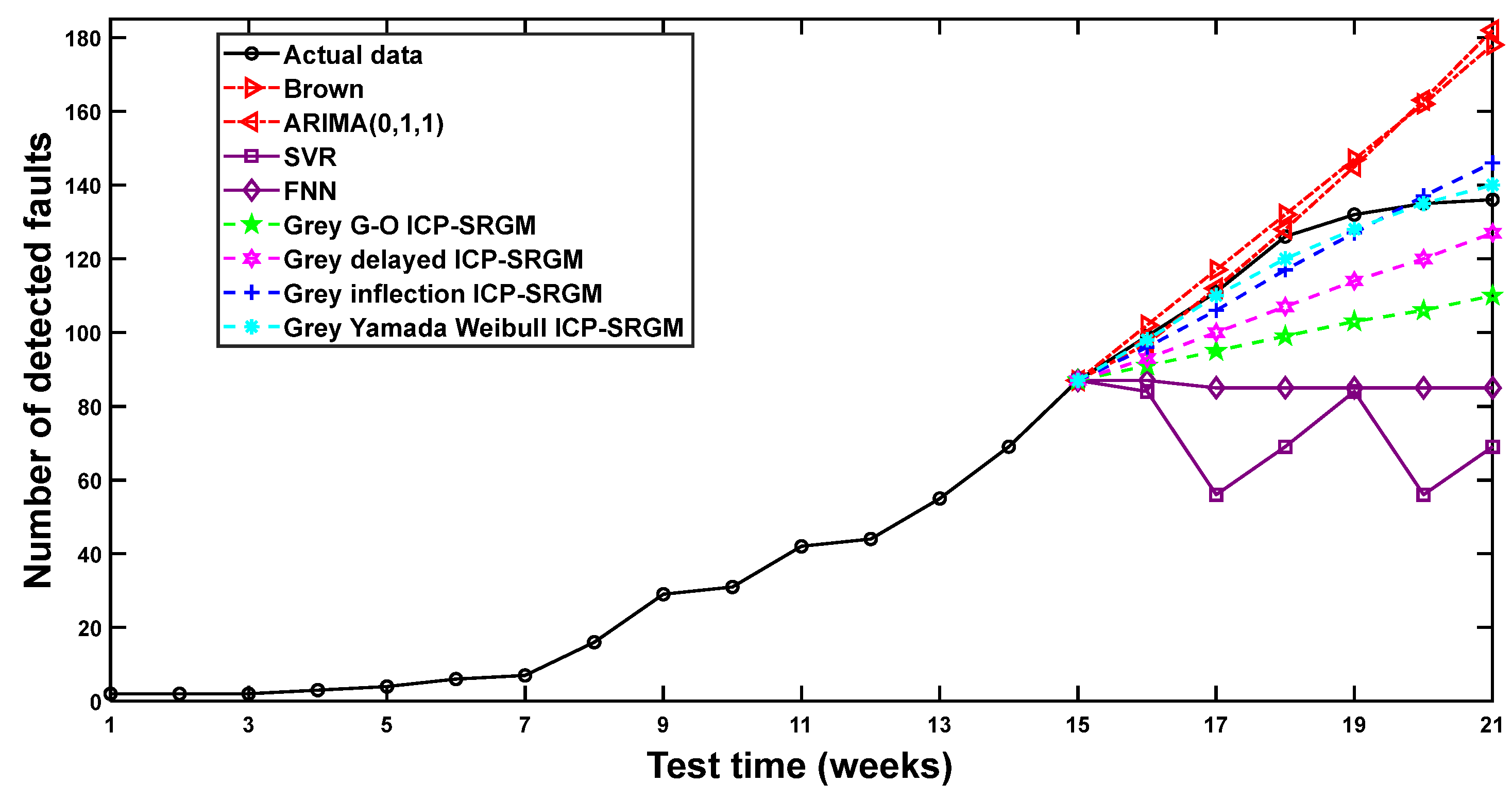
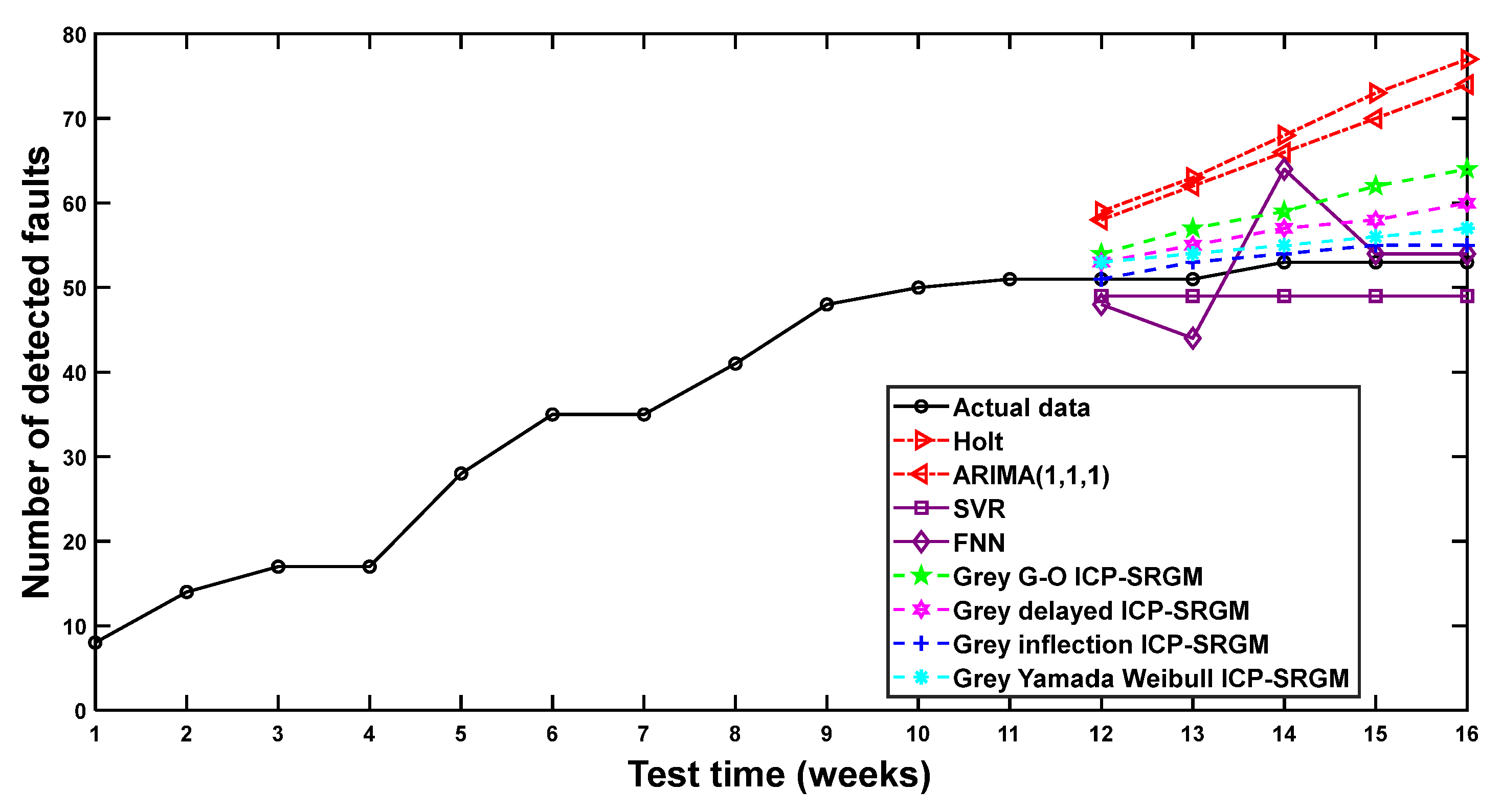
Figure 1 and Figure 2 depict the prediction results of the number of detected faults in DS1 and DS2 for all comparison models, respectively, and the corresponding MAPE values are reported in

Table 6. The prediction error of the number of detected faults in DS1 for all comparison models (MAPE: %).

Test Weeks	Holt-ES	ARIMA (1,1,1)	SVR	FNN	Grey GO ICP	Grey Delayed ICP	Grey Inflection ICP	Grey Weibull ICP
12	15.69	13.73	3.92	5.88	5.88	3.92	0.00	3.92
13	23.53	21.57	3.92	13.73	11.76	7.84	3.92	5.88
14	28.30	24.53	7.55	20.75	11.32	7.55	1.89	3.77
15	37.74	32.08	7.55	1.89	16.98	9.43	3.77	5.66
16	45.28	39.62	7.55	1.89	20.75	13.21	3.77	7.55
Average	30.11	26.30	6.10	8.83	13.34	8.39	2.67	5.36

and

Table 7. The prediction error of the number of detected faults in DS2 for all comparison models (MAPE: %).

Test Weeks	Brown-ES	ARIMA (0,1,1)	SVR	FNN	Grey GO ICP	Grey Delayed ICP	Grey Inflection ICP	Grey Weibull ICP
16	3.03	2.02	15.15	12.12	8.08	6.06	3.03	1.01
17	5.41	0.90	49.55	23.42	14.41	9.91	4.50	0.90
18	4.76	1.59	45.24	32.54	21.43	15.08	7.14	4.76
19	11.36	9.85	36.36	35.61	21.97	13.64	3.79	3.03
20	20.00	20.74	58.52	37.04	21.48	11.11	1.48	0.00
21	30.88	33.82	49.26	37.50	19.12	6.62	7.35	2.94
Average	12.57	11.49	42.35	29.70	17.75	10.40	4.55	2.11

.

Table 6 and Figure 1 show that, in DS1, grey inflection ICP-SRGM has the best prediction results, followed by grey Weibull ICP-SRGM and grey delayed ICP-SRGM. The prediction results of SVR are also good, while the prediction performance of FNN is not ideal. Based on time series analysis, the Holt-ES model and ARIMA model have the worst prediction results.

Table 7 and Figure 2 show that, in DS2, the prediction result of grey Yamada Weibull ICP-SRGM is the best, followed by grey inflection ICP-SRGM. The predictive performance of SVR and FNN is not ideal. Based on time series analysi, the Brown-ES model and ARIMA model show good prediction results in the early weeks, but their prediction bias increases in the later weeks.

4. Discussion

The experimental results demonstrate that the proposed grey ICP-SRGM framework consistently outperforms both the original grey SRGMs and some conventional prediction methods.

The grey ICP-SRGMs improve prediction accuracy over the original grey SRGMs (Table 4 and Table 5). This improvement can be attributed to the explicit incorporation of the fault correction process. The original grey SRGM framework assumes perfect debugging [11], i.e., every detected fault is immediately and correctly removed. This assumption is often violated in real software testing, where correction may be delayed or imperfect. By directly using the collected corrected fault data and introducing a fault correction rate function, the proposed grey ICP-SRGM framework captures the imperfect nature of the correction process, leading to more realistic predictions.

As shown in Figure 1 and Figure 2 and summarized in Table 6 and Table 7, the proposed grey ICP-SRGM framework yields more stable short-term predictions than time series models (Brown-ES, Holt-ES, ARIMA) and machine learning models (SVR, FNN). This is mainly because it is better suited to small sample data and grouped data. Time series models rely on stationarity assumptions and tend to deviate significantly in later prediction steps, whereas machine learning models, especially FNN, require large amounts of data and suffer from overfitting when training data are limited. In contrast, the grey ICP-SRGM framework is designed to extract trend information from limited data without relying on large datasets [20]. This makes it particularly practical for early-stage software testing, when only a few weeks of fault data are available [26,27].

The choice of the fault correction rate function also plays a critical role in model performance. Among the five candidate functions evaluated (Table 2), the logistic-type function $p_4(t)$ achieves the lowest MAPE and RMSE for both DS1 and DS2. This S-shaped curve reflects a common trend in practice: correction efficiency tends to increase gradually as testers become more familiar with the software, and it eventually stabilizes [31]. In contrast, a constant or exponential form may fail to capture such a behavior. Therefore, when applying the grey ICP-SRGM framework in practice, the fault correction rate function should be selected based on the actual correction data rather than prescribed arbitrarily.

Despite these positive findings, several limitations should be acknowledged. First, the proposed grey ICP-SRGM framework assumes that no new faults are introduced during the correction process, which may not be realistic in complex development environments. Second, the proposed framework is specifically designed for small sample data (sequence length ≤ 25) and grouped data; for exact failure time data or large sample cases, other approaches such as time series models or machine learning methods may be more suitable.

5. Conclusions

This paper proposed a new grey SRGM that integrates both fault detection and correction processes, denoted as the grey ICP-SRGM framework. Unlike the original grey SRGM framework that assumes perfect debugging, the proposed model directly incorporates corrected fault counts and employs a one-step iterative estimation method. Numerical experiments on two real datasets demonstrated that the grey ICP-SRGM framework significantly improves prediction accuracy over the original grey SRGM on four specific model forms (grey G-O, grey delayed, grey inflection, and grey Yamada Weibull). Compared with time series models (Brown-ES, Holt-ES, ARIMA) and machine learning models (SVR, FNN), the proposed framework exhibits superior short-term predictive performance, particularly in cases with small samples and grouped data. These findings confirm that the proposed grey ICP-SRGM framework is practical and effective for software reliability assessment, especially when data availability is limited, such as in the early stages of testing or when only grouped fault counts are recorded.

As for future work, several promising directions warrant further investigation. These include relaxing the assumption that no new faults are introduced during correction to account for imperfect debugging, extending the framework to handle change points and time-varying testing efforts, and validating the model on a wider range of open-source and industrial projects, along with comparisons against more recent deep learning approaches.

References

1. Nor, A.K.M.; Pedapati, S.R.; Muhammad, M. Reliability engineering applications in electronic, software, nuclear and aerospace industries: A 20-year review (2000–2020). Ain Shams Eng. J. 2021, 12, 3009–3019. [Google Scholar] [CrossRef]
2. Oveisi, S.; Moeini, A.; Farsi, M. Software reliability prediction: A survey. Qual. Reliab. Eng. Int. 2023, 39, 412–453. [Google Scholar]
3. Oveisi, S.; Moeini, A.; Mirzaei, S.; Farsi, M.A. Software reliability prediction: A machine learning and approximation Bayesian inference approach. Qual. Reliab. Eng. Int. 2024, 40, 4004–4037. [Google Scholar] [CrossRef]
4. Pandey, S.K.; Mishra, R.B.; Tripathi, A.K. Machine Learning Based Methods for Software Fault Prediction: A Survey. Expert Syst. Appl. 2021, 172, 114595. [Google Scholar] [CrossRef]
5. Samal, U.; Kumar, A. Enhancing Software Reliability Forecasting Through a Hybrid ARIMA-ANN Model. Arab. J. Sci. Eng. 2024, 49, 7571–7584. [Google Scholar]
6. Anand, A.; Yamada, S.; Tamura, Y.; Yadav, A. On the utility of approximation methods for analyzing software error detection phenomenon. Qual. Reliab. Eng. Int. 2025, 41, 3244–3257. [Google Scholar] [CrossRef]
7. Hou, Y.F.; Huang, C.Y.; Fang, C.C. Using the Methods of Statistical Data Analysis to Improve the Trustworthiness of Software Reliability Modeling. IEEE Access 2022, 10, 25358–25375. [Google Scholar] [CrossRef]
8. Khan, F.M.; Munir, A.; Albaity, M.; Nadeem, M.; Mahmood, T. Software Reliability Growth Model Selection by Using VIKOR Method Based on q-Rung Ortho pair Fuzzy Entropy and Divergence Measures. IEEE Access 2024, 12, 86572–86582. [Google Scholar] [CrossRef]
9. Liu, Z.; Yang, S.K.; Yang, M.H.; Kang, R. Software belief reliability growth model based on uncertain differential equation. IEEE Trans. Reliab. 2022, 71, 775–787. [Google Scholar] [CrossRef]
10. Liu, Z.; Kang, R. Imperfect debugging software belief reliability growth model based on uncertain differential equation. IEEE Trans. Reliab. 2022, 71, 735–746. [Google Scholar] [CrossRef]
11. Liu, X.M.; Xie, N.M. Grey-based approach for estimating software reliability under nonhomogeneous Poisson process. J. Syst. Eng. Electron. 2022, 33, 360–369. [Google Scholar] [CrossRef]
12. Goel, A.L.; Okumoto, K. Time dependent error-detection rate model for software reliability and other performance measures. IEEE Trans. Softw. Eng. 1979, 28, 206–211. [Google Scholar] [CrossRef]
13. Chang, I.H. NHPP software reliability model with rayleigh fault detection rate and optimal release time for operating environment uncertainty. Appl. Sci. 2024, 14, 10072. [Google Scholar] [CrossRef]
14. Song, K.Y.; Chang, I.H. An NHPP-based software reliability model with time-dependent fault detection rate under uncertain operating environments. J. Korean Data Inf. Sci. Soc. 2025, 36, 587–596. [Google Scholar] [CrossRef]
15. Qbal, J.; Nazir, R.; Rasool, T. NHPP-based testing coverage model with fault removal efficiency and error generation. Int. J. Reliab. Qual. Saf. Eng. 2025, 32, 1–16. [Google Scholar]
16. Musa, J.D.; Iannino, A.; Okumoto, K. Software Reliability: Measurement, Prediction, Application; McGraw-Hill: Columbus, OH, USA, 1990. [Google Scholar]
17. Hsu, C.J.; Huang, C.Y.; Chang, J.R. Enhancing software reliability modeling and prediction through the introduction of time variable fault reduction factor. Appl. Math. Model. 2011, 35, 506–521. [Google Scholar] [CrossRef]
18. Pachauri, B.; Dhar, J.; Kumar, A. Incorporating inflection S-shaped fault reduction factor to enhance software reliability growth. Appl. Math. Model. 2015, 39, 1463–1469. [Google Scholar] [CrossRef]
19. Chatterjee, S.; Shukla, A. Modeling and analysis of software fault detection and correction process through Weibull-type fault reduction factor, Change Point and Imperfect Debugging. Arab. J. Sci. Eng. 2016, 41, 5009–5025. [Google Scholar] [CrossRef]
20. Deng, J. Grey System Theory Course; Huazhong University of Science and Technology Press: Wuhan, China, 1990; pp. 175–378. (In Chinese) [Google Scholar]
21. Toga, G.; Atalay, B.; Toksari, M.; Forrest, J. Solving U-type assembly line balancing under grey uncertainties: Grey learning effect and grey task times approach. Grey Syst. 2025, 15, 462–477. [Google Scholar] [CrossRef]
22. Xie, N.; Qin, Y.; Chen, N.; Yang, Y. Single batch-processing machine scheduling problem with interval grey processing time. Appl. Soft Comput. 2025, 170, 112661. [Google Scholar] [CrossRef]
23. Wang, X.; Liu, X.; Huang, Y.; Chang, C.; Guo, J. Multivariate Fractional Grey Model for Port Throughput Prediction. J. Grey Syst. 2025, 37, 23–32. [Google Scholar]
24. Wang, X.; Xie, N.; Yang, L.; Wei, B. Grey forecasting modelling for deteriorating inventory with interdependent quality and quantity decay. Expert Syst. Appl. 2026, 306, 130956. [Google Scholar] [CrossRef]
25. Zhao, K.; Wu, L. Heterogeneity grey model and its prediction of energy consumption under the shared socioeconomic pathways. Energy 2025, 319, 134851. [Google Scholar] [CrossRef]
26. Dong, W.; Deng, S.; Chen, C.; Li, K.; Yang, Y. Predicting residual fault times in reliability growth management under limited failure data set. Qual. Technol. Quant. Manag. 2026, 23, 458–474. [Google Scholar]
27. Dong, W.; Guo, J.; Liu, L.; Yang, Y. Terminating the Reliability Growth Test Under Small Sample Failure Dataset. IEEE Trans. Reliab. 2025, 74, 4832–4841. [Google Scholar] [CrossRef]
28. Shibata, K.; Rinsaka, K.; Dohi, T.; Okamura, H. Quantifying software maintainability based on a fault-detection/correction model. In Proceedings of the 13th Pacific Rim International Symposium on Dependable Computing (PRDC 2007), Melbourne, VIC, Australia, 17–19 December 2007; pp. 35–42. [Google Scholar]
29. Lo, J.-H.; Huang, C.-Y. An integration of fault detection and correction processes in software reliability analysis. J. Syst. Softw. 2006, 79, 1312–1323. [Google Scholar] [CrossRef]
30. Yamada, S.; Ohba, M.; Osaki, S. S-shaped reliability growth modeling for software error detection. IEEE Trans. Reliab. 1983, 32, 475–484. [Google Scholar] [CrossRef]
31. Yamada, S.; Ohba, M.; Osaki, S. S-shaped software reliability growth models and their applications. IEEE Trans. Reliab. 1984, 33, 289–292. [Google Scholar] [CrossRef]
32. Yamada, S.; Hishitani, J. Software reliability growth with a Weibull test effort: A model and application. IEEE Trans. Reliab. 1993, 42, 100–106. [Google Scholar] [CrossRef]
Figure 1. Prediction results of the number of detected faults in DS1 for all comparison models.
Processes 14 02197 g001
Figure 2. Prediction results of the number of detected faults in DS2 for all comparison models.
Processes 14 02197 g002