Transmission Line Fault Diagnosis Based on Time–Frequency-Domain Recurrence Plots and CNN-BiGRU-Attention

Abstract

Rapid and accurate identification of various faults occurring in transmission lines is essential for restoring normal line operation. However, existing transmission line fault diagnosis methods still face challenges in terms of noise immunity and diagnostic accuracy. To address these issues, this paper proposes a deep learning method based on recurrence plots and a convolutional neural network–bidirectional gated recurrent unit–attention mechanism model. The voltage and current signals of transmission lines are transformed into recurrence plots in both the time and frequency domains. Parallel convolutional neural networks are then employed to extract local features from the two domains, while bidirectional gated recurrent units are used to capture temporal dependencies. Furthermore, multi-head self-attention and cross-attention mechanisms are introduced to enhance key features within each domain and achieve adaptive fusion of inter-domain feature information. A transmission line model is established in Simulink to collect data under various fault conditions and influencing factors, thereby verifying the effectiveness and adaptability of the proposed method. Experimental results show that the proposed method achieves fault recognition accuracies of 99.63%, 96.68%, and 75.38% under NL1, NL2, and NL3 Gaussian-noise conditions, respectively, and maintains accuracies of 99.02%, 95.93%, and 72.43% under mixed-noise conditions. Compared with other deep learning models, the proposed method demonstrates higher diagnostic accuracy and stronger robustness.

1. Introduction

With the continuous growth of electricity demand and the expanding scale of interconnected power systems, transmission lines, as essential carriers for long-distance power delivery, play a critical role in ensuring the security and stability of modern power grids [1]. Since transmission lines are exposed to complex natural environments for long periods, they are prone to faults caused by lightning strikes, ice accretion, insulator contamination, external-force damage, extreme weather, and other disturbances [2]. Typical transmission line faults include three-phase short-circuit faults, single-phase-to-ground faults, phase-to-phase faults, and double-phase-to-ground faults [3]. Different fault types exhibit distinct transient impact characteristics, nonlinear evolution patterns, and multichannel coupling relationships in three-phase voltage and current signals. Therefore, rapidly and accurately extracting effective features from complex fault signals and realizing intelligent identification of multiple fault types are essential prerequisites for the safe and stable operation of power systems.

With the development of smart grids, increasingly stringent requirements have been imposed on the real-time performance and intelligence of transmission line fault diagnosis. Representative deep learning methods mainly include convolutional neural networks (CNNs) and recurrent neural networks (RNNs). CNNs have attracted extensive attention owing to their strong capability for automatic feature learning [4]. Their main advantage lies in the weight-sharing mechanism of convolution operations [5], which can significantly reduce the number of trainable parameters and model complexity. However, due to the limitation of fixed receptive fields [6], CNNs generally have difficulty capturing long-term dependencies in complex sequential data. RNNs model temporal dependencies through recurrent structures [7]. Nevertheless, during backpropagation, gradients need to be repeatedly multiplied across multiple time steps, which may lead to gradient vanishing or gradient explosion [8], thereby weakening the ability of the model to learn long-term dependencies. As an improved RNN variant, the gated recurrent unit (GRU) introduces update and reset gates [9] to dynamically regulate information transmission and forgetting. Therefore, GRU can more effectively capture long-term dependencies and alleviate the vanishing gradient problem to a certain extent.

In practical operating environments, monitoring signals used for fault diagnosis are inevitably affected by complex noise caused by corona discharge, switching operations, electromagnetic transients, measurement errors, and other disturbances. Noise may obscure key fault-related features and significantly degrade the diagnostic performance of deep learning algorithms. To address this issue, time–frequency recurrence plots have been introduced into fault diagnosis. By reconstructing the phase space, a recurrence plot (RP) can describe the recurrence relationships among system states and transform one-dimensional signals into two-dimensional images with dynamic similarity structures, thereby revealing nonlinear dynamic features that are difficult to observe directly from raw waveforms or conventional time–frequency maps [10,11]. However, most existing studies directly transform complete time-series samples into a single large-scale recurrence plot. Although this strategy can preserve the global dynamic information of signals, it may weaken local transient variations at the early stage of faults and introduce redundant image information and additional computational burden. Consequently, it is not conducive to the fine extraction of local fault textures and stage-wise evolution characteristics by deep learning models.

Attention mechanisms assign different weights to different features, thereby highlighting important information while suppressing irrelevant components [12]. They can effectively improve model performance and have become an important concept in deep learning, with early successful applications in computer vision and image processing. In 2017, Vaswani et al. [13] proposed the Transformer architecture, in which the self-attention (SA) mechanism can better capture long-range dependencies and significantly improve computational parallelism. Li et al. [14] introduced self-attention into fault detection to reduce the interference of nonlinear and noisy information while enhancing the influence of fault-related key information in samples. Guo et al. [15] integrated a multi-head self-attention (MHSA) module with CNN to improve the model’s ability to focus on discriminative features of fault signals. In addition, CNN–RNN hybrid models and attention-enhanced models have gradually been applied to fault diagnosis of mechanical and electrical equipment. Related studies have shown that attention mechanisms can emphasize key features and suppress redundant information, thereby improving classification performance [16,17]. However, in most existing CNN–long short-term memory (LSTM)–Attention-based methods, attention mechanisms are mainly applied within a single feature space and focus primarily on intra-sequence weight allocation or local feature enhancement. The adaptive interaction between time-domain transient evolution features and frequency-domain energy distribution features remains insufficiently considered.

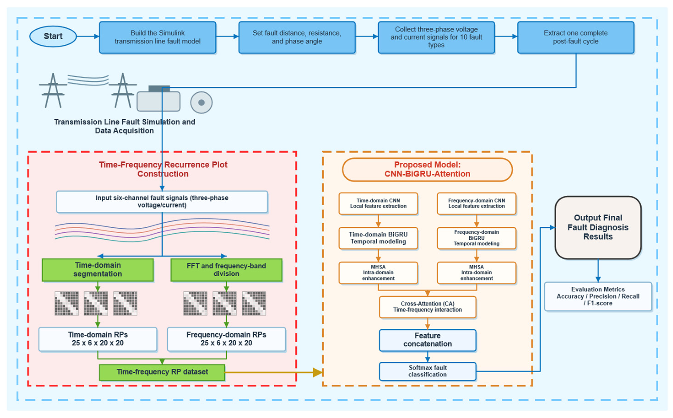
To address the above issues, this study proposes a transmission line fault diagnosis method based on time–frequency-domain recurrence plots and a CNN–bidirectional gated recurrent unit (BiGRU)–Attention model. First, before constructing recurrence plots, the time-domain signals are segmented, and frequency-domain sub-band division is further performed to generate time-domain and frequency-domain recurrence plots, respectively. This strategy not only reduces the input size of each recurrence plot, but also preserves local dynamic characteristics in different temporal segments and frequency sub-bands, providing a more structured input for subsequent CNN-based local feature extraction and BiGRU-based inter-segment dependency modeling. Second, a dual-branch CNN-BiGRU feature extraction network is designed. Specifically, CNN is used to extract local spatial features from recurrence plots, while BiGRU is employed to model bidirectional temporal dependencies among different recurrence plot segments. Third, a multi-head self-attention mechanism is introduced to adaptively enhance key features within the time and frequency domains, improving the model’s ability to focus on effective fault-related information. Furthermore, a cross-attention (CA) mechanism is adopted to establish interactions between time-domain and frequency-domain features, enabling the fusion of complementary cross-domain information. Finally, multiple types of transmission line faults are identified through feature concatenation and a Softmax classifier.

The main contributions of this paper are summarized as follows:

(1)

A time–frequency-domain recurrence plot representation method is proposed for transmission line fault diagnosis. The three-phase voltage and current signals are processed in a segmented manner and then mapped into two-dimensional recurrence plots in both the time and frequency domains. This representation preserves the dynamic evolution information of faults while enhancing the model’s ability to characterize nonlinear fault features and spectral distribution patterns.

(2)

A dual-branch CNN-BiGRU deep feature extraction model is constructed. CNN is used to extract local spatial features from recurrence plots, while BiGRU captures bidirectional temporal dependencies among different segments, thereby improving the model’s learning capability for complex fault patterns.

(3)

Multi-head self-attention and cross-attention mechanisms are introduced to achieve intra-domain key feature enhancement and adaptive fusion of time–frequency-domain features, respectively. These mechanisms strengthen the model’s comprehensive discriminative capability for multichannel, multiscale, and strongly coupled fault information.

2. Relevant Theories

2.1. Recurrence Plot

The recurrence plot is a classical signal processing method whose core principle is to transform a one-dimensional time series into a two-dimensional image by characterizing recurrence relationships, thereby enabling visualization of the phase-space structure of a dynamical system. Based on Takens’ embedding theorem, the original sequence $\left\{x_1,x_2,\dots ,x_i\right\}$ is reconstructed into a series of phase-space vectors by selecting an appropriate embedding dimension $a$ and delay time $d$. By calculating the recurrence relationships among these reconstructed vectors, a recurrence plot can be generated for subsequent feature analysis and fault diagnosis.

$$X_i=\left(x_i,x_{i+d},\dots ,x_{i+\left(a-1\right)d}\right)$$

(1)

The Euclidean distance between two vectors in the recurrence plot is calculated according to Equation (2). Here, $\epsilon$ denotes the distance threshold between two points in the phase space, $\theta$ represents the Heaviside function, $\Vert ·\Vert$ indicates the Euclidean norm, and $X_i$ and $X_j$ are the state vectors at specific time instants.

$$R{P}_{i,j}=\theta \left(\epsilon -\Vert X_i-X_j\Vert \right)$$

(2)

In this study, recurrence plots are not used merely for visualization. They are used to convert short post-fault voltage and current segments into two-dimensional texture-like representations. Different fault types produce different recurrence structures because of their distinct nonlinear transient evolution. Therefore, RP provides an effective representation for CNN-based local pattern extraction.

2.2. Fast Fourier Transform

The fast Fourier transform (FFT) [18] is an efficient algorithm for computing the discrete Fourier transform (DFT) and its inverse transform. In signal processing, the DFT transforms a signal from the time domain into the frequency domain, thereby clearly revealing its spectral components and serving as a fundamental tool for spectral analysis. However, the computational cost of directly calculating the DFT increases quadratically with the number of data points, which has long limited its practical application in engineering scenarios involving large-scale or long-duration signals.

The FFT algorithm decomposes the complete DFT matrix into a product of a series of sparse matrices, as expressed in Equation (3), thereby reducing the computational complexity. FFT not only enables real-time frequency-domain analysis of complex signals but also greatly expands the application scope of digital signal processing.

$$A_k={\displaystyle \sum _{n=0}^{N-1}} {\mathrm{e}}^{-{\displaystyle \frac{\mathrm{i}2\pi kn}{N}}}x\left(t\right)$$

(3)

where $x\left(t\right)$ denotes the time-domain signal, and $A_k$ represents the frequency-domain signal obtained by applying the discrete Fourier transform to $x\left(t\right)$.

FFT is introduced before frequency-domain RP construction to reveal the spectral redistribution caused by fault transients. This compensates for the limitation of time-domain RPs, which mainly describe temporal evolution but cannot directly represent frequency-domain energy distribution.

2.3. Convolutional Neural Network

A convolutional neural network is a multilayer neural network consisting of an input layer, convolutional layers, pooling layers, and fully connected layers [19]. Its typical architecture is shown in Figure 1. The convolutional layer is the core component of CNN, and its main function is to perform convolution operations on the input data using convolution kernels and then pass the resulting feature maps to the next layer of the network. The convolution operation is expressed as Equation (4):

$$y_i^l=\delta \times \left(w_i^l\times X^{l-1}+b_i^l\right)$$

(4)

where $y_i^l$ denotes the $i$-th feature map of the $l$-th layer, $\delta$ is the activation function, $w_i^l$ represents the weight matrix of the $i$-th convolution kernel in the $l$-th layer, × denotes the convolution operation, ${\mathrm{X}}^{l-1}$ is the output of the $(l-1)$-th layer, and $b_i^l$ is the bias term.

After the convolutional layer, an activation function is applied to introduce nonlinear characteristics into the output data, thereby enhancing the feature representation capability of the model. The rectified linear unit (ReLU), as a nonlinear unsaturated activation function, is widely used in CNN models owing to its fast convergence speed and simple gradient calculation. The ReLU function is defined as follows:

$$f_{cov}\left(y_i^l\right)=\mathrm{m}\mathrm{a}\mathrm{x}\left(0,y_i^l\right)$$

(5)

A pooling layer is subsequently introduced to reduce the number of model parameters and suppress overfitting while retaining the prominent features of the output data. The commonly used global average pooling operation is expressed as Equation (6):

$$f_i^{l+1}\left(j\right)=GAP\left\{f_{cov}\left(y_i^l\right)\right\}$$

(6)

where $f_i^{l+1}\left(j\right)$ denotes the $j$-th element of the $i$-th feature map in the ($l+1$)-th layer after average pooling.

The fully connected layer serves as the final classification module of the CNN model. It uses the extracted features after nonlinear activation to generate the probability distribution of each class. The Softmax function is adopted as the final output of the model:

$$p\left(f_j\right)={\displaystyle \frac{\exp \left(f_j\right)}{{\sum }_{k=1}^m\exp \left(f_k\right)}}$$

(7)

where $f_j$ denotes the output of the $j$-th neuron in the output layer, $m$ is the number of fault categories, and $p\left(f_j\right)$ represents the probability output of the neuron after the Softmax function.

The generated RP is a two-dimensional image-like representation, and the convolution operation can extract local recurrence textures and spatial correlations from each RP segment.

2.4. Gated Recurrent Unit

The gated recurrent unit, originally proposed by Cho et al. [20], has emerged as an effective variant of recurrent neural networks (RNNs). GRU addresses the inherent vanishing gradient problem of traditional RNNs and incorporates the memory capability of long short-term memory (LSTM) networks. Meanwhile, owing to its reduced number of trainable parameters, GRU generally achieves faster computational efficiency during training. A GRU consists of two gates, namely the reset gate and the update gate, as shown in Figure 2, which are used to regulate information transmission.

Both gates receive the hidden state ${\mathrm{h}}_{\mathrm{t}-1}$ from the previous time step and the current input ${\mathrm{x}}_{\mathrm{t}}$, and generate gating vectors with values ranging from 0 to 1 through the weight matrices and the Sigmoid activation function. The update gate ${\mathrm{Z}}_{\mathrm{t}}$ determines the extent to which the previous hidden state ${\mathrm{h}}_{\mathrm{t}-1}$ is replaced by the candidate hidden state. A larger value of ${\mathrm{Z}}_{\mathrm{t}}$ indicates a higher contribution of the candidate state to the current hidden state. The reset gate ${\mathrm{R}}_{\mathrm{t}}$ controls the contribution of the previous hidden state ${\mathrm{h}}_{\mathrm{t}-1}$ when generating the candidate hidden state. A smaller value of ${\mathrm{h}}_{\mathrm{t}-1}$ indicates that more historical information is forgotten. The update gate and reset gate are expressed as follows:

$${\mathrm{Z}}_{\mathrm{t}}=\sigma \left({\mathrm{W}}_{\mathrm{z}}\left[{\mathrm{h}}_{\mathrm{t}-1},{\mathrm{x}}_{\mathrm{t}}\right]\right)$$

(8)

$${\mathrm{R}}_{\mathrm{t}}=\sigma \left({\mathrm{W}}_{\mathrm{r}}\left[{\mathrm{h}}_{\mathrm{t}-1},{\mathrm{x}}_{\mathrm{t}}\right]\right)$$

(9)

The candidate hidden state ${\tilde{\mathrm{h}}}_{\mathrm{t}}$ is generated by combining the current input ${\mathrm{x}}_{\mathrm{t}}$, the previous hidden state ${\mathrm{h}}_{\mathrm{t}-1}$, and the output of the reset gate ${\mathrm{R}}_{\mathrm{t}}$, as shown in Equation (10). The final hidden state ${\mathrm{h}}_{\mathrm{t}}$ is then determined according to the output of the update gate, as expressed in Equation (11). Here, ${\mathrm{W}}_{\mathrm{h}}$ denotes the weight matrix of the candidate hidden state, and $\mathrm{t}\mathrm{a}\mathrm{n}\mathrm{h}$ is the activation function.

$${\tilde{\mathrm{h}}}_{\mathrm{t}}=\tanh \left({\mathrm{W}}_{\mathrm{h}}\left[{\mathrm{R}}_{\mathrm{t}}\times {\mathrm{h}}_{\mathrm{t}-1},{\mathrm{x}}_{\mathrm{t}}\right]\right)$$

(10)

$${\mathrm{h}}_{\mathrm{t}}=\left(1-{\mathrm{Z}}_{\mathrm{t}}\right)\times { \mathrm{h}}_{\mathrm{t}-1}+{\mathrm{Z}}_{\mathrm{t}}\times {\tilde{\mathrm{h}}}_{\mathrm{t}}$$

(11)

Since each sample consists of RP segments, the extracted CNN features form a segment-level sequence. BiGRU is used to model the dependencies among these RP segments in both forward and backward directions.

2.5. Transformer

2.5.1. Multi-Head Self-Attention

Multi-head self-attention [21] is a core component of the Transformer architecture. Its basic principle is to learn the attention weights of each position in a given input sequence and then perform a weighted summation of the input sequence based on these weights.

Specifically, the input sequence F is first mapped into the query matrix Q, key matrix K, and value matrix V through three learnable weight matrices, namely $W_Q$, $W_K$, and $W_V$, respectively. The attention scores are then calculated by performing dot-product operations between Q and K. Subsequently, the scores are scaled and normalized using the Softmax function to obtain the attention weights. These attention weights are multiplied by the value matrix V, and the weighted results over all positions are summed to generate the contextual representation. Finally, multiple sets of query, key, and value projections are used to compute the contextual representations of different attention heads in parallel, and the outputs of all heads are concatenated to form the final multi-head attention representation. The calculation process is expressed as follows, where $\mathrm{h}$ denotes the number of attention heads.

$$Q=\mathrm{F}{W}_Q; K=\mathrm{F}{W}_K; V=\mathrm{F}{W}_V$$

(12)

$${\mathrm{Score}}_{\mathrm{i}}=\mathrm{Attention}\left({\mathrm{Q}}_{\mathrm{i}},\mathrm{K},\mathrm{V}\right)$$

(13)

$${\mathrm{Attention}\text{\_}\mathrm{Weights}}_{\mathrm{i}}=\mathrm{softmax}\left({\mathrm{Score}}_{\mathrm{i}}\right)$$

(14)

$${\mathrm{C}}_{\mathrm{i}}={\displaystyle \sum _{\mathrm{j}=1}^{\mathrm{n}}} {\mathrm{Attention}\text{\_}\mathrm{Weights}}_{\mathrm{j}}\cdot {\mathrm{V}}_{\mathrm{j}}$$

(15)

$$\mathrm{MultiHead}\left(\mathrm{X}\right)=\mathrm{Concat}\left({\mathrm{C}}_1,{\mathrm{C}}_2,\dots ,{\mathrm{C}}_{\mathrm{h}}\right)$$

(16)

2.5.2. Cross-Attention

Cross-attention computes attention between two different sequences and is commonly used to fuse features from different sequences [22]. By modeling complex interactions across different feature spaces, cross-attention enhances the overall representational capability of the model. Its core computational process is similar to that of multi-head self-attention, but it differs in the generation of the query, key, and value matrices. As expressed in Equation (17), $F_1$ and $F_2$ denote two different input sequences.

$$\begin{array}{c}Q=F_1{W}_Q; K=F_2{W}_K; V=F_2{W}_V\end{array}$$

(17)

MHSA is used for intra-domain feature enhancement, while CA is used for inter-domain feature interaction. Therefore, attention mechanisms in this paper are not merely used as a classifier enhancement module but as a feature selection and fusion mechanism for time–frequency complementary information.

2.6. Evaluation Metrics

To comprehensively evaluate the experimental results of transmission line fault diagnosis, Accuracy, Precision, Recall, and F1-score are adopted as evaluation metrics in this paper. The definitions of these metrics are given as follows:

$$\mathrm{Accuracy}={\displaystyle \frac{\mathrm{T}P+\mathrm{T}N}{TP+FP+TN+FN}}$$

(18)

$$\mathrm{Prec}\mathrm{i}\mathrm{sion}={\displaystyle \frac{TP}{TP+FP}}$$

(19)

$$\mathrm{Recall}={\displaystyle \frac{TP}{TP+FN}}$$

(20)

$$F1-\mathrm{score}=2\times {\displaystyle \frac{\mathrm{Prec}\mathrm{i}\mathrm{sion}\times \mathrm{Recall}}{\mathrm{Prec}\mathrm{i}\mathrm{sion}+\mathrm{Recall}}}$$

(21)

Here, TP denotes the number of fault-state signals that are correctly identified as fault signals by the model; TN denotes the number of normal-state signals that are correctly identified as normal signals; FN denotes the number of fault-state signals that are incorrectly identified as normal signals; and FP denotes the number of normal-state signals that are incorrectly identified as fault signals.

3. Fault Diagnosis Process

3.1. Acquisition of Transmission Line Fault Signals

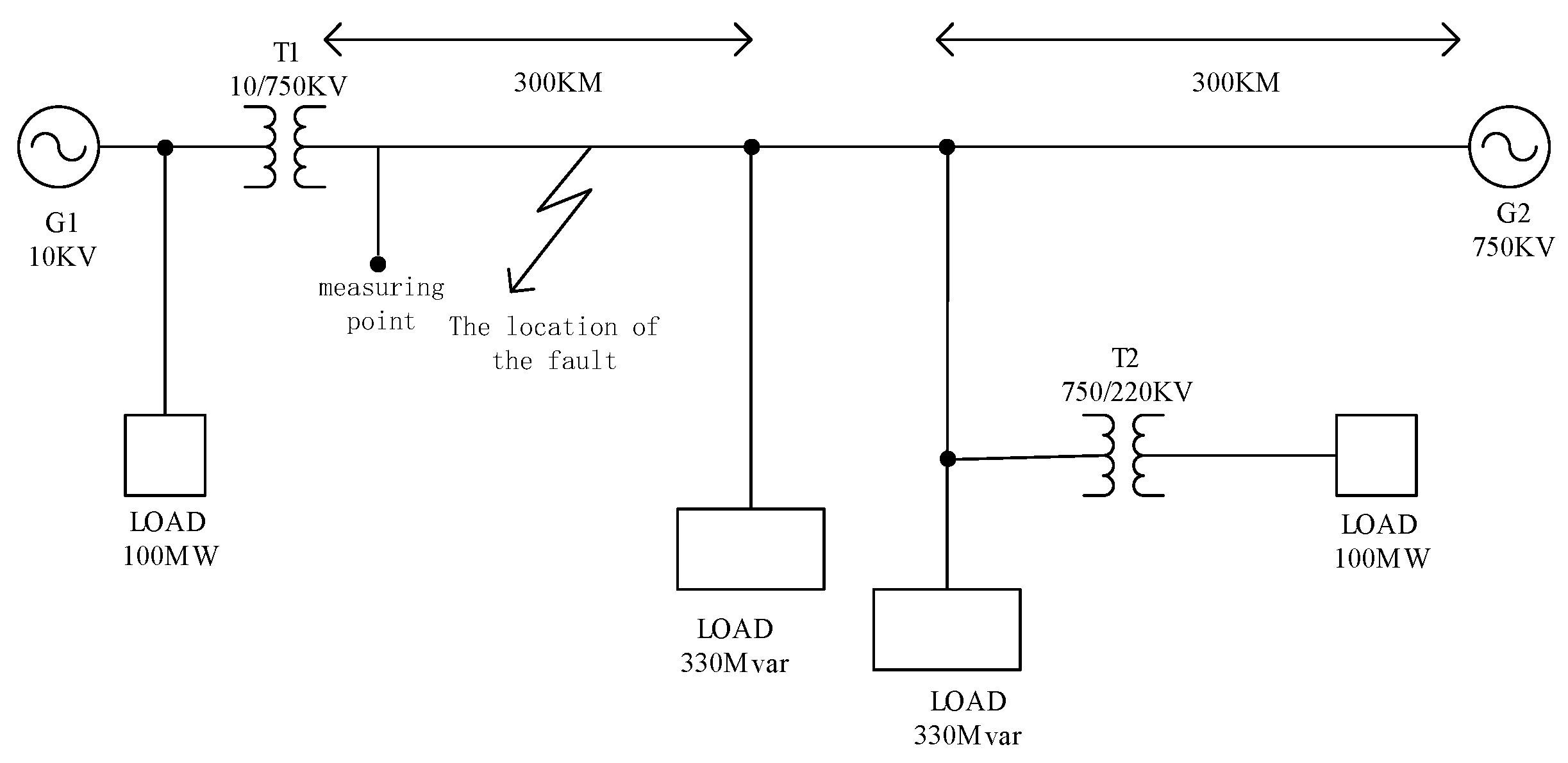
The transmission line fault simulation system was established using the Simulink simulation platform [23], as shown in Figure 3. At the sending end, six synchronous generator units, each with a rated power of 350 MVA and an output voltage of 10 kV, were connected to the system. The voltage was increased to 750 kV through step-up transformers. The transmission network consisted of two 300 km long transmission lines. A regional load of 100 MW was connected at the sending end, while the receiving end supplied power to a 220 kV distribution network through step-down transformers. In addition, two groups of centralized reactive power compensation devices with a capacity of 330 Mvar were installed to maintain voltage stability.

A fault simulation module was configured to simulate ten types of faults, including single-phase-to-ground faults (AG, BG, and CG), double-phase-to-ground faults (ABG, ACG, and BCG), phase-to-phase faults (AB, BC, and AC), and three-phase-to-ground faults (ABCG). The measurement module was arranged at the B1 side of the generator to record three-phase voltage and current data. In each measurement, three phase-voltage signals and three phase-current signals were obtained, resulting in a total of six fault-related signals.

In practical transmission lines, fault scenarios are complex and highly variable. To simulate different fault conditions, simulation experiments were conducted under different fault locations, fault resistances, and fault inception angles, with the parameter settings listed in

Table 1. Settings of fault parameters.

Simulation Parameters	Training Set	Testing Set
Fault distance (KM)	20 40 60 80 100 120 140 160 180 200 220 240 280	30 50 70 90 110 130 150 170 190 210 230 250 270
Fault resistance (Ω)	0.1 1 10 20 30 40 50 60 70 80 100	0.1 5 15 25 35 45 90
Fault inception angle (°)	0 30 120 150 210 270 300 330	60 90 180 240

. The training and testing sets were divided in a partially non-overlapping manner to verify the generalization capability of the proposed model under unseen fault parameters. The system sampling frequency was set to 20 kHz, and the simulation duration was 0.2 s. After random combinations of the simulation parameters, a total of 15,080 groups of three-phase voltage and current signal data were collected, covering ten fault types.

To improve computational efficiency and focus on critical fault-related features, one complete cycle of data after fault inception was extracted from each simulated sample, corresponding to approximately 333 sampling points and containing the transient characteristics at the early stage of the fault. For each fault type, 1144 groups of three-phase voltage and current signal data were used for training, and 364 groups were used for testing.

3.2. Time–Frequency Recurrence Plot Transformation

To address the problem of high-dimensional feature extraction and representation of transmission line fault signals, this paper proposes a time–frequency-domain analysis method based on RPs. Directly transforming the original multi-channel fault signals into RPs may produce excessively large images and increase computational complexity. Moreover, large-scale RPs generated from the entire signal may contain redundant information and are not conducive to effective feature extraction by CNNs. Therefore, a segment-wise RP construction strategy is adopted in both the time domain and the frequency domain.

In this study, The embedding dimension and delay time are set to their default values, namely $a$ = 1 and $d$ = 1, respectively. Under this setting, each sampling point is directly regarded as a state vector, and no additional phase-space expansion is performed. Therefore, for each 20-point time-domain segment or 20-point frequency-domain amplitude sequence, the number of state vectors remains 20, resulting in a recurrence plot with a size of (20 × 20). This setting is consistent with the input size required by the subsequent CNN model and avoids additional resizing operations for short signal segments.

In addition, the recurrence threshold is set to None in the implementation. Therefore, the generated recurrence plots are not binarized. Instead, the pairwise distances between state vectors are retained to form continuous recurrence representations. Compared with binary recurrence plots, this strategy preserves more detailed distance information and avoids the information loss that may be caused by manually selecting a hard threshold. Since no binary thresholding is applied, the recurrence threshold is not treated as an additional tunable parameter in this study.

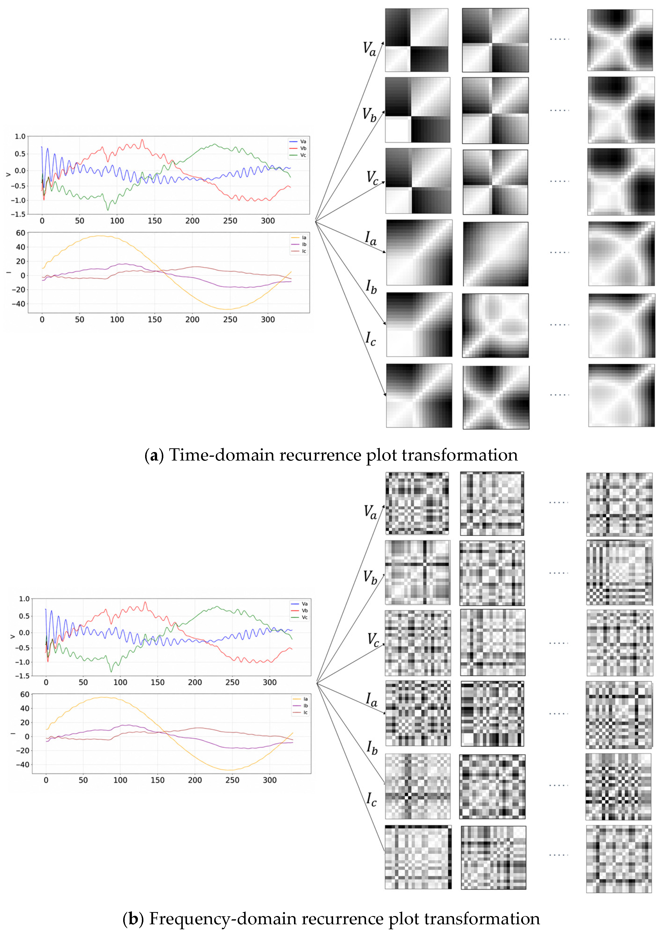
The time-domain processing procedure is shown in Figure 4a. Each of the six signal channels is segmented independently. For each channel, 25 time windows are selected from one complete post-fault cycle, and the length of each window is set to 20 sampling points. These 25 windows are uniformly selected so that the main transient variation process after fault inception can be covered. For each time-domain segment with a length of 20, RP transformation is performed separately, thereby mapping the one-dimensional segment into a 20 × 20 two-dimensional recurrence image. Therefore, the time-domain RP representation of one fault sample can be expressed as 25 × 6 × 20 × 20, where 25 denotes the number of selected time windows, 6 denotes the number of signal channels, and 20 × 20 denotes the size of the RP generated from each segment.

The frequency-domain processing procedure is shown in Figure 4b. First, the FFT is applied to each channel independently to obtain the corresponding amplitude spectrum. Considering that the main spectral information of fault transient signals is mainly concentrated in the low-frequency range, the frequency range of 0–1500 Hz is selected for frequency-domain analysis. This frequency range is uniformly divided into 25 sub-bands, and the bandwidth of each sub-band is 60 Hz. For each sub-band and each channel, the corresponding spectral amplitude sequence is extracted.

Since the number of discrete frequency points contained in different frequency sub-bands may vary, the amplitude sequences in all sub-bands are normalized to a unified length of 20. This length normalization is performed only to standardize the input size required for RP construction and the subsequent neural network model, rather than to introduce additional physical frequency components. When the number of frequency points in a sub-band is fewer than 20, linear interpolation is used to resample the amplitude sequence into a 20-point sequence. When the number of frequency points in a sub-band is not fewer than 20, the first 20 amplitude points are selected as the feature sequence of the sub-band. Then, RP transformation is applied to each 20-point frequency-domain amplitude sequence separately, mapping it into a 20 × 20 two-dimensional frequency-domain RP. Consequently, the frequency-domain RP representation of one fault sample can be expressed as 25 × 6 × 20 × 20, where 25 denotes the number of frequency sub-bands, 6 denotes the number of signal channels, and 20 × 20 denotes the size of the RP generated from each frequency-domain amplitude sequence.

Before being input into the dual-branch CNN-BiGRU network, the six-channel RPs corresponding to the same segment index are stacked along the channel dimension. Therefore, each segment is represented as a six-channel RP image with a spatial size of 20 × 20. For the time-domain branch, the input sequence is composed of 25 segment-level six-channel RP images, which can be denoted as 25 × 6 × 20 × 20. For the frequency-domain branch, the input sequence is similarly composed of 25 sub-band-level six-channel RP images, which can be denoted as 25 × 6 × 20 × 20. In this representation, the CNN is used to extract spatial texture features from each six-channel RP image, while the BiGRU is used to learn the sequential dependencies among the 25 time-domain segments or 25 frequency-domain sub-bands.

3.3. Workflow of the Fault Diagnosis Algorithm

The overall workflow of the proposed algorithm mainly consists of five components: feature extraction, time–frequency-domain feature enhancement, time–frequency-domain feature interaction and feature concatenation, as illustrated in Figure 5.

(1)

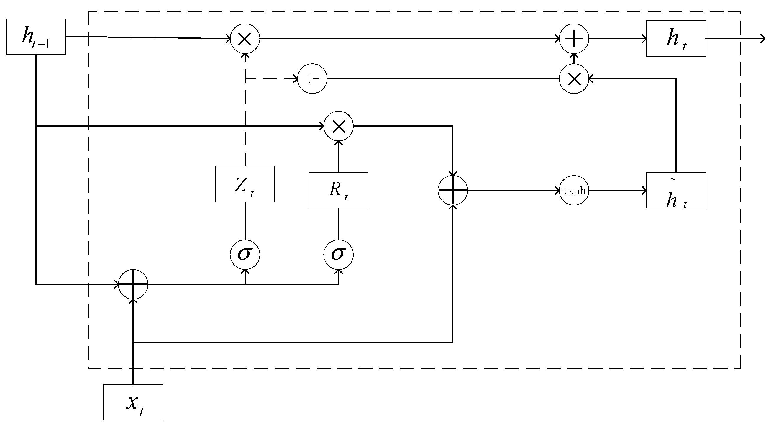
Feature extraction: First, convolutional layers are employed to extract features from the time- and frequency-domain inputs, thereby capturing local patterns and spatial correlations within each RP segment. Subsequently, a BiGRU layer is introduced to model the long-term dependencies among different RP segments. The GRU learns sequence-level relationships among segmented RP representations, while the bidirectional structure enables the model to capture both forward and backward contextual information.

(2)

Time–frequency-domain feature enhancement: A multi-head self-attention mechanism is adopted in both the time-domain and frequency-domain branches to enhance the feature representation within each domain. By calculating the correlation weights among the queries, keys, and values, the self-attention mechanism enables the model to focus on informative segments and adaptively aggregate global contextual information. As a result, the discriminative representation capability of each branch is improved.

(3)

Time–frequency-domain feature interaction: Time-domain and frequency-domain features describe the same fault state from different perspectives. The time-domain features mainly characterize the transient evolution process after fault inception, whereas the frequency-domain features provide complementary spectral information, such as frequency distribution and energy variation. Since these two types of features are heterogeneous but correlated, direct feature concatenation may be insufficient to explicitly model their cross-domain dependencies. Therefore, before the final feature fusion stage, a cross-attention mechanism is designed to establish adaptive interaction between the time and frequency domains.

In the proposed cross-attention module, the enhanced time-domain feature is used as the query, while the enhanced frequency-domain feature is used as the key and value. This design is based on the consideration that post-fault transient waveforms provide direct diagnostic cues for fault evolution. By using the time-domain feature as the query, the model can selectively retrieve and integrate frequency-domain components that are highly relevant to the current transient pattern. In this way, the contribution of frequency-domain information is no longer combined with the time-domain information using fixed fusion weights, but is adaptively determined according to the time-domain diagnostic context. In addition, different from direct feature concatenation, the proposed cross-attention mechanism explicitly models the dependency between the two domains before feature fusion. Therefore, it can suppress redundant or weakly related spectral components while enhancing complementary time–frequency representations.

(4)

Feature concatenation: After obtaining the enhanced time-domain feature, the enhanced frequency-domain feature, and the cross-domain interaction feature generated by the cross-attention module, these features are concatenated to form the final fused representation. It should be noted that the concatenation operation at this stage is not a direct concatenation of the original time- and frequency-domain features. Instead, it is performed after intra-domain feature enhancement and cross-domain adaptive interaction. Therefore, the fused representation can preserve domain-specific information while incorporating complementary time–frequency interaction information.

3.4. Model Parameter Settings

The proposed model was implemented in Python 3.9 on a Windows 11 operating system, with an NVIDIA RTX 4060 GPU used for acceleration. The Adam optimizer was adopted for model training, with an initial learning rate of 0.0005, a batch size of 32, and 100 training epochs. The model complexity was calculated after the network construction using the same input dimensions as those adopted in the experiments, where the time-domain and frequency-domain recurrence plot inputs were both represented as tensors of 25 × 6 × 20 × 20. The total number of parameters of the proposed model was approximately 6.40 × 10⁶. The saved model file size was approximately 25.6 MB. In addition, the computational cost of a single forward inference was approximately 2.96 × 10⁸ FLOPs, corresponding to approximately 1.48 × 10⁸ MACs. The detailed model parameter settings are listed in

Table 2. Part of the network layer parameter settings.

Network Layer	Parameter
CNN layer	kernel number = 16, kernel size = 3 × 3, padding = same; BatchNormalization; activation function: ReLU
Recurrent layer	Bidirectional GRU; units number = 64; return sequences = True; dropout = 0.2; recurrent dropout = 0.2
Multi-head self-attention layer	head number = 4; key dimension = 32
Cross-attention layer	head number = 4; key dimension = 32
FC layer	neurons number = 128; activation function: ReLU
Softmax layer	neurons number = 10; activation function: Softmax

.

4. Comparison and Analysis of Experimental Results

4.1. Simulation of Noisy Environments

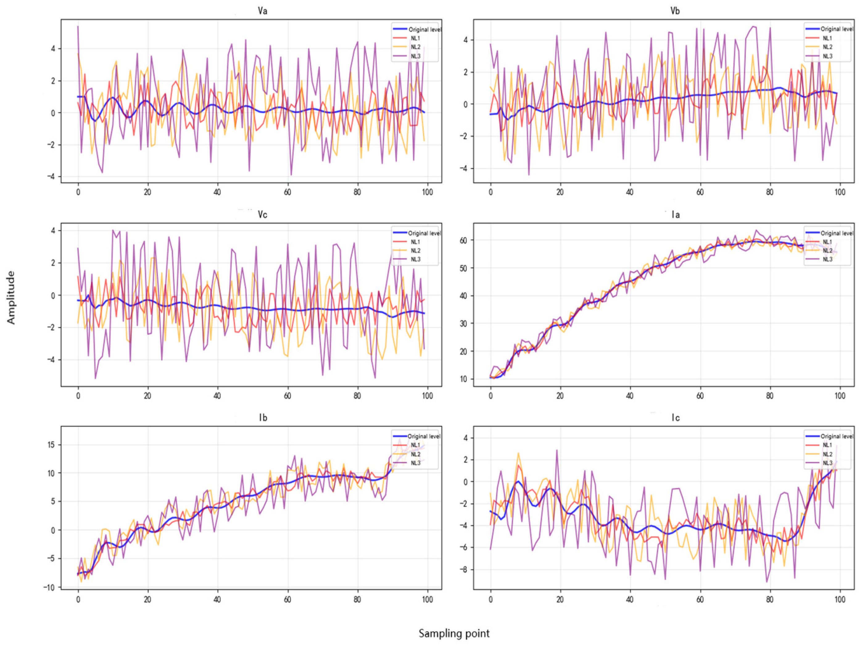
In practical operation, transmission line fault signals are susceptible to noise interference generated by other operating equipment, such as electromagnetic interference and corona discharge. Therefore, the noise immunity of the fault-classification model is crucial for ensuring reliable classification performance. In this paper, Gaussian noise with different signal-to-noise ratios (SNRs) is added to the testing dataset to simulate various noisy environments and evaluate the anti-noise capability of the proposed model. The noisy three-phase voltage and current signals are shown in Figure 6, where NL1, NL2, and NL3 denote Gaussian noise levels with SNRs of 25 dB, 20 dB, and 15 dB, respectively.

To further investigate the robustness of different fault-classification methods under more challenging operating conditions, mixed-noise scenarios are additionally considered for comparative experiments. Specifically, harmonic noise with SNRs of 25 dB, 20 dB, and 15 dB is superimposed on the Gaussian-noise-contaminated signals corresponding to NL1, NL2, and NL3, respectively. The resulting mixed-noise levels are denoted as ML1, ML2, and ML3. Under these conditions, the testing signals are simultaneously affected by random Gaussian noise and periodic harmonic interference, providing a more realistic representation of the complex noise environment encountered in practical transmission line operation.

The intensity of noise is represented by the signal-to-noise ratio, as expressed in (22), where $P_N$ denotes the effective power of the noise and $P_S$ denotes the effective power of the signal.

$$\mathrm{S}\mathrm{N}\mathrm{R}=10\mathrm{l}\mathrm{g}{\displaystyle \frac{P_S}{P_N}}$$

(22)

4.2. Results of Fault Diagnosis

In this paper, a confusion matrix is used to visually evaluate and analyze the fault classification performance of the proposed model. A confusion matrix is a classification performance evaluation tool in which the rows represent the true classes of the samples and the columns represent the predicted classes of the model. The elements on the diagonal of the matrix indicate the number of correctly classified samples, whereas the off-diagonal elements reflect misclassified samples. Therefore, the confusion matrix can intuitively demonstrate the classification performance of the model across different categories.

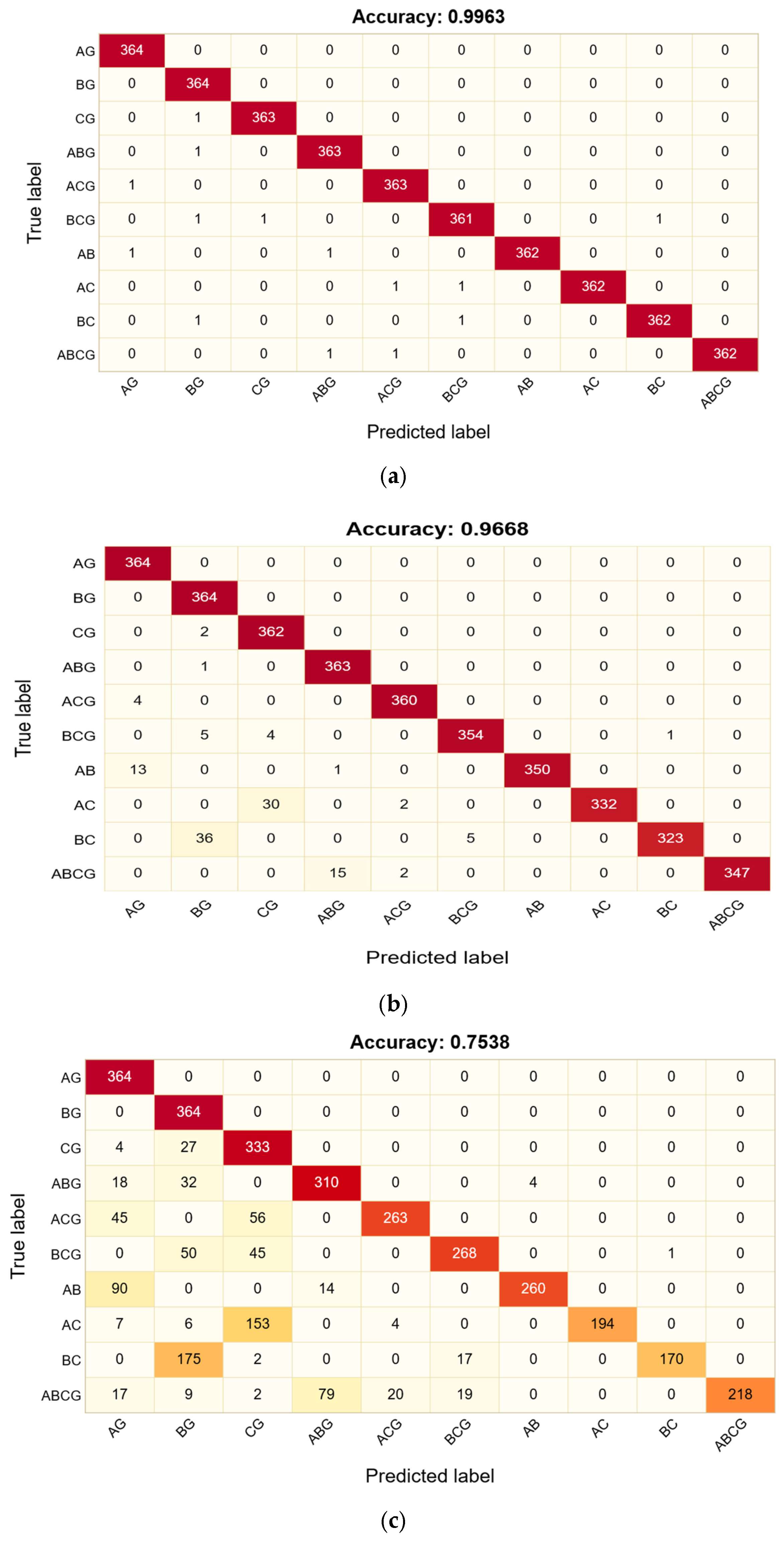
The experimental results are shown in Figure 7. Under the NL1 noise condition, the proposed model achieves an accuracy of 99.63%. Under the NL2 noise condition, although the model is affected by noise interference, it still achieves an accuracy of 96.68%. Under the more severe NL3 noise condition, the model suffers from stronger noise interference, and its accuracy decreases to 75.38%.

In addition, to evaluate whether the proposed method can meet the real-time requirements of practical power-system fault diagnosis, the computational time of the main processing stages was measured on the experimental platform described in Section 3.4. The total diagnosis time for a single sample can be expressed as:

$$T_{total}=T_{data}+T_{RP-time}+T_{RP-FFT}+T_{Inference}$$

(23)

where $T_{data}$ denotes the data acquisition time, $T_{RP-time}$ denotes the time-domain RP construction time, $T_{RP-FFT}$ denotes the FFT-based frequency-domain processing time, and $T_{Inference}$ denotes the neural network inference time.

Since the sampling frequency of the system is 20 kHz and one complete post-fault cycle contains approximately 333 sampling points, the data acquisition time is approximately 16.65 ms. The measured time-domain RP construction time is 3.33 ms, the FFT-based frequency-domain processing time is 17.93 ms, and the network inference time is 6.64 ms. Therefore, the total diagnosis time is calculated as 44.55 ms. These results demonstrate the potential of the proposed method for online fault diagnosis.

4.3. Ablation Experiments

To verify the contribution of each improved module to model performance, ablation experiments were designed in this paper. The effects of bidirectional feature learning, the multi-head self-attention mechanism (MHSA), and the cross-attention mechanism (CA) on the fault diagnosis performance of the model were analyzed, and the experimental results are presented in

Table 3. Results of the ablation experiments.

Model	NL1 (%)	NL2 (%)	NL3 (%)
CNN-GRU	97.28	70.34	40.88
CNN-BiGRU	98.74	73.22	46.62
MHSA-CNN-BiGRU	99.17	78.35	51.65
CA-CNN-BiGRU	98.84	74.54	49.57
MHSA-CA-CNN-BiGRU	99.63	96.68	75.38

. Under the low-noise condition NL1, all models achieve high recognition accuracy, ranging from 97.28% to 99.63%. This indicates that when noise interference is relatively weak, the basic CNN-GRU structure can effectively extract fault features and achieve accurate classification. However, as the noise level increases from NL1 to NL2 and NL3, the performance differences among different models gradually become more pronounced, suggesting that structural improvements play an important role in enhancing model robustness under complex noisy environments.

Compared with CNN-GRU, CNN-BiGRU improves the accuracy by 1.46%, 2.88%, and 5.74% under NL1, NL2, and NL3, respectively. This demonstrates that BiGRU can simultaneously model forward and backward temporal dependencies, thereby enhancing the model’s ability to represent dynamic fault characteristics. After further introducing the MHSA module, MHSA-CNN-BiGRU achieves accuracies of 99.17%, 78.35%, and 51.65% under NL1, NL2, and NL3, respectively, representing improvements of 0.43%, 5.13%, and 5.03% over CNN-BiGRU. These results indicate that the multi-head self-attention mechanism can effectively capture long-range feature dependencies and significantly improve the discriminative capability of the model under increased noise interference.

The CA-CNN-BiGRU model, which only introduces the CA module, achieves accuracies of 98.84%, 74.54%, and 49.57% under NL1, NL2, and NL3, respectively. Compared with CNN-BiGRU, the accuracy is improved by 0.10%, 1.32%, and 2.95%, indicating that the cross-attention mechanism can promote interaction and fusion among different types of feature information to a certain extent, thereby improving fault recognition accuracy. However, compared with MHSA-CNN-BiGRU, its accuracy under NL2 and NL3 remains slightly lower.

Finally, the MHSA-CA-CNN-BiGRU model, which integrates both MHSA and CA modules, achieves the best performance under all three noise conditions, with accuracies of 99.63%, 96.68%, and 75.38%, respectively. Compared with the models using only MHSA or CA, the complete model obtains higher classification accuracy, indicating that the two attention modules make complementary contributions to the overall diagnostic performance. It should be noted that this study mainly evaluates the contribution of the attention mechanisms from the perspective of classification performance through ablation experiments.

4.4. Comparative Experiments

Based on the proposed time–frequency-domain recurrence plot representation and CNN-BiGRU-Attention model, transmission line fault diagnosis is conducted under different noisy environments. Eight representative models, including LSTM, CNN, SVM, TCN, CNN-LSTM-MHSA, CNN-LSTM-CA, CNN-Transformer, and Vision Transformer, are selected as baseline methods for comparison. The diagnostic accuracies under Gaussian-noise conditions are listed in

Table 4. Diagnostic accuracy comparison of different models under gaussian noisy environments.

Model	NL1 (%)	NL2 (%)	NL3 (%)
LSTM	82.01	76.42	46.39
CNN	89.20	69.62	23.65
SVM	96.02	41.62	10.12
TCN	82.69	69.88	31.66
CNN-LSTM-MHSA	93.30	45.52	21.51
CNN-LSTM-CA	90.71	45.30	28.93
CNN-Transformer	96.95	55.14	23.71
Vision-Transformer	84.89	73.93	60.69
Proposed	99.63	96.68	75.38

, while the results under mixed-noise conditions are presented in

Table 5. Diagnostic accuracy comparison of different models under mix noisy environments.

Model	ML1 (%)	ML2 (%)	ML3 (%)
LSTM	79.22	70.39	40.59
CNN	87.93	65.41	20.37
SVM	95.06	40.80	10.77
TCN	81.08	66.88	29.16
CNN-LSTM-MHSA	92.97	44.04	20.52
CNN-LSTM-CA	90.16	44.64	28.65
CNN-Transformer	96.16	54.60	22.04
Vision-Transformer	84.22	72.09	58.90
Proposed	99.02	95.93	72.43

.

As shown in Table 4, the proposed method achieves an accuracy of 99.63% under the low Gaussian-noise condition NL1, outperforming all baseline models. When the noise intensity increases to NL2 and NL3, the performance of all models decreases to different extents. Nevertheless, the proposed method still obtains accuracies of 96.68% and 75.38%, respectively, showing superior robustness under stronger Gaussian noise.

To further evaluate the robustness of different models under more complex interference, mixed-noise scenarios are introduced by combining Gaussian noise with harmonic noise. As reported in Table 5, the proposed method achieves the highest accuracies of 99.02%, 95.93%, and 72.43% under ML1, ML2, and ML3, respectively. Although the mixed-noise conditions cause additional performance degradation compared with the Gaussian-noise cases, the proposed model consistently maintains the best diagnostic accuracy among all compared methods. This indicates that the proposed method has strong resistance to both random noise and periodic harmonic interference.

In addition to accuracy, Precision, Recall, and F1-score are calculated to provide a more comprehensive evaluation of classification performance. The detailed metric comparisons under Gaussian-noise conditions are given in

Table 6. Comparison of diagnostic metrics, including Precision, Recall, and F1-score, among different models under gaussian noisy environments.

Model	NL1			NL2			NL3
	Precision	Recall	F1-Score	Precision	Recall	F1-Score	Precision	Recall	F1-Score
LSTM	0.82	0.81	0.81	0.76	0.78	0.77	0.46	0.47	0.46
CNN	0.89	0.90	0.89	0.75	0.71	0.72	0.24	0.23	0.23
SVM	0.96	0.95	0.95	0.35	0.48	0.40	0.10	0.11	0.10
TCN	0.83	0.82	0.82	0.79	0.59	0.67	0.22	0.41	0.28
CNN-LSTM-MHSA	0.94	0.93	0.93	0.78	0.45	0.57	0.35	0.20	0.25
CNN-LSTM-CA	0.91	0.90	0.90	0.49	0.45	0.47	0.36	0.28	0.31
CNN-Transformer	0.96	0.96	0.96	0.61	0.55	0.57	0.23	0.23	0.23
Vision-Transformer	0.89	0.89	0.89	0.79	0.74	0.76	0.71	0.61	0.65
Proposed	0.99	0.99	0.99	0.97	0.96	0.96	0.83	0.75	0.78

, and those under mixed-noise conditions are shown in

Table 7. Comparison of diagnostic metrics, including Precision, Recall, and F1-score, among different models under mix various noisy environments.

Model	ML1			ML2			ML3
	Precision	Recall	F1-Score	Precision	Recall	F1-Score	Precision	Recall	F1-Score
LSTM	0.80	0.79	0.79	0.72	0.69	0.70	0.41	0.40	0.40
CNN	0.87	0.87	0.87	0.66	0.65	0.65	0.20	0.20	0.20
SVM	0.95	0.95	0.95	0.44	0.41	0.42	0.10	0.10	0.10
TCN	0.81	0.81	0.81	0.69	0.66	0.67	0.33	0.29	0.31
CNN-LSTM-MHSA	0.93	0.92	0.92	0.65	0.44	0.52	0.47	0.20	0.28
CNN-LSTM-CA	0.91	0.90	0.90	0.48	0.44	0.46	0.35	0.28	0.31
CNN-Transformer	0.97	0.97	0.97	0.74	0.56	0.64	0.31	0.25	0.28
Vision-Transformer	0.88	0.85	0.86	0.77	0.72	0.74	0.69	0.59	0.64
Proposed	0.99	0.99	0.99	0.96	0.95	0.95	0.77	0.72	0.74

. Under NL1, the proposed method achieves 0.99 for Precision, Recall, and F1-score. Under NL2 and NL3, it obtains 0.97/0.96/0.96 and 0.83/0.75/0.78 in terms of Precision, Recall, and F1-score, respectively, which are higher than those of the baseline models.

Furthermore, as shown in Table 7, the proposed method also maintains the best overall performance under mixed-noise conditions. Specifically, the Precision, Recall, and F1-score reach 0.99/0.99/0.99 under ML1, 0.96/0.95/0.95 under ML2, and 0.77/0.72/0.74 under ML3, respectively. These results demonstrate that the proposed model not only achieves high classification accuracy but also maintains a favorable balance between Precision and Recall under severe noise interference.

Overall, the above comparisons verify that the proposed CNN-BiGRU-Attention model combined with time–frequency-domain recurrence plot representation has superior anti-interference capability. By integrating CNN-based feature extraction, BiGRU-based temporal dependency modeling, and attention-based key information enhancement, the proposed framework effectively improves the reliability and stability of transmission line fault diagnosis in complex noisy environments.

5. Conclusions

To address the problem of transmission line fault diagnosis, this paper proposes a fault diagnosis method based on time–frequency-domain recurrence plots and a CNN-BiGRU-Attention model. The proposed model is constructed by introducing time–frequency-domain recurrence plot representation, bidirectional feature learning, and attention-based feature enhancement. Its performance is experimentally validated using a transmission line fault dataset. The experimental results demonstrate the following conclusions:

(1)

The proposed method maintains stable classification accuracy under variations in fault resistance, fault inception angle, and fault location, and exhibits good performance in noisy environments.

(2)

The construction of time–frequency-domain recurrence plot datasets, together with the integration of the CNN-BiGRU architecture and attention mechanisms, enables the model to learn discriminative fault-related representations from fault signals. The ablation experiments show that the introduction of MHSA and CA improves the classification accuracy of the overall network. These results indicate that the attention modules contribute positively to the proposed fault diagnosis framework.

(3)

Compared with other classical methods, the proposed method achieves the highest classification accuracy on the transmission line fault dataset, demonstrating the superiority of the time–frequency-domain recurrence plot and CNN-BiGRU-Attention-based fault diagnosis method.

Although the experimental results demonstrate that the proposed method achieves high diagnostic accuracy and robustness under different simulated fault conditions, some limitations still remain. First, the data used in this study are mainly generated from a MATLAB/Simulink simulation model. Although various fault distances, fault resistances, fault inception angles, and noise conditions are considered to enhance the diversity of the dataset, field-measured fault data from practical transmission lines are still lacking. Therefore, the generalization capability and engineering applicability of the proposed method need to be further verified using real operating data. Second, the current CNN-BiGRU-Attention model involves recurrence plot generation, dual-branch feature extraction, and attention-based feature fusion. Although the proposed method shows potential for online fault diagnosis, the model structure can still be further optimized for deployment in resource-constrained protection devices. In future work, lightweight model design, including model compression, pruning, knowledge distillation, and efficient attention mechanisms, will be investigated to reduce computational cost while maintaining diagnostic accuracy and robustness.