Article

Multi-Objective Optimization of Multi-Cooperative Agricultural Machinery Scheduling Under Continuous Workload Sharing: A Hybrid Particle Swarm–Tabu Search Approach


1
Key Laboratory of Modern Agricultural Equipment, Ministry of Agriculture and Rural Affairs, Nanjing 210014, China
2
School of Mechanical Engineering, Nanjing Institute of Technology, Nanjing 211167, China
3
Nanjing Institute of Agricultural Mechanization, Ministry of Agriculture and Rural Affairs, Nanjing 210014, China
*
Author to whom correspondence should be addressed.
Processes 2026, 14(13), 2181; https://doi.org/10.3390/pr14132181
Submission received: 9 June 2026 / Revised: 28 June 2026 / Accepted: 2 July 2026 / Published: 3 July 2026

Abstract

Coordinating a shared fleet across multiple owners under tight time windows is a challenging multi-objective problem balancing cost, timeliness, and equity. We study it for multi-cooperative agricultural machinery dispatch, formulating the Multi-Cooperative Agricultural Machinery Scheduling Problem under Continuous Workload Sharing (MAMSP-CWS) as a three-objective model that minimizes inter-area transfer cost, time-window violation, and cross-cooperative workload imbalance. To approximate the Pareto front, we develop a Multi-Objective Hybrid Particle Swarm Optimization with Tabu Search and Sparsity Repair (MO-HPSO-TS-SR), which couples particle-swarm search, tabu-search refinement, and a sparsity-repair operator within an external crowding-distance archive. The method is evaluated on three scales (a real instance from Liyang, China, and two synthetic ones) against NSGA-II-CWS and HTSMOGA-CWS over 20 independent runs each. MO-HPSO-TS-SR attains the best mean value on every metric-by-scale combination, with a decisive convergence advantage (hypervolume and IGD; Holm-adjusted p < 0.001 , Cliff’s δ 1 ). A mechanism decomposition identifies Sparsity Repair as the dominant contributor to hypervolume, with Tabu Search as a complementary refiner. The advantage over NSGA-II-CWS widens with problem scale, from 19.4% on the Small instance to 74.2% on the Large instance, reflecting the disproportionate degradation of the genetic baseline rather than a growing advantage of the proposed method. Beyond agriculture, the framework extends to other continuous-encoding scheduling problems, providing a transferable decision-support tool.

1. Introduction

Coordinating a shared pool of mobile machines across spatially distributed, time-critical tasks is a recurring problem in operations and process systems engineering, arising wherever capacity must be pooled across organizational boundaries to meet deadlines under limited resources. Agricultural machinery dispatch during the peak harvest is a particularly demanding instance of this problem class. Over the past two decades, the mechanization of cereal harvesting in China has evolved from a singular, on-farm activity into a logistically coordinated multi-stakeholder operation: as family-scale landholdings have consolidated through agricultural-cooperative arrangements and machinery investment has shifted from individual ownership to fleet pooling, dispatching combine harvesters now requires the coordinated assignment and routing of machines across multiple cooperatives and multiple time-critical fields simultaneously [1], a setting in which transportation cost, operational timeliness, and workload balance must be reconciled at once. During the peak wheat-harvesting window in a major grain-producing province such as Jiangsu in the lower Yangtze River basin, several thousand hectares may require harvesting within roughly ten days, so that the operational efficiency of the cooperative network, rather than the absolute number of machines, becomes the binding constraint on timely completion. Even modest dispatching inefficiencies translate into substantial losses through prolonged transit, missed agronomic windows, and inequitable workload distribution across member cooperatives. The Multi-Cooperative Agricultural Machinery Scheduling Problem (MAMSP) therefore constitutes a problem class of both considerable scale and pressing practical importance.
In our prior work [2], we introduced the Continuous Workload Sharing (CWS) encoding—a representational innovation that permits a single field to be partitioned among multiple machines through a continuous workload-share variable rather than a single binary assignment. The CWS encoding better reflects actual cooperative practice during peak season, when several harvesters routinely converge on a large field to meet a narrow harvesting deadline; it also expands the optimizer’s feasible region by removing the structural restriction of one machine per field. There, we coupled this encoding with a Hybrid Particle Swarm Optimizer (HPSO) and demonstrated significant improvements over conventional Genetic Algorithm and Simulated Annealing baselines on a single-objective formulation that combined transfer cost, time-window penalty, and operational cost into a weighted scalar surrogate.
While our single-objective formulation [2] yields a tractable target, it inherits the fundamental limitation of weighted-sum approaches: the manager’s preferences must be fixed before the problem’s trade-offs are known. The relative weighting of transfer cost, time-window penalty, and workload equity is, in practice, a contextual decision shaped by weather risk, contractual obligations, inter-cooperative considerations, and other factors that vary across operations, seasons, and regions. A planner consulting a single optimized schedule cannot see how it would change under a different weighting, nor reason quantitatively about marginal trade-offs. Moreover, because cost, timeliness, and structural regularity are folded into one scalar, the single-objective setting cannot reveal how these concerns trade off against one another. The present work retains the CWS encoding, the MAMSP setting, the Sparsity Repair operator, and the Liyang dataset of [2], and departs from it in three respects. First, it recasts the single weighted-sum objective as a three-objective Pareto formulation that additionally captures cross-cooperative workload equity. Second, it augments the particle-swarm search with Tabu Search local refinement and an external Pareto archive, converting the single-objective optimizer of [2] into a Pareto-front method. Third, it re-examines Sparsity Repair under multiple objectives, where a mechanism-level decomposition shows that its structural pruning trades a small timeliness loss for reductions in transfer cost and workload imbalance, an effect that a single scalar cannot expose.
In parallel, the multi-objective evolutionary computation literature has produced sophisticated frameworks for navigating problems with competing objectives. Among these, the Hybrid Tabu Search Multi-Objective Genetic Algorithm (HTSMOGA) of Guo et al. [3] for bi-objective agricultural scheduling demonstrates that multi-objective formulations of farming-logistics problems are both feasible and informative—exposing rich Pareto-front structures that single-objective surrogates would obscure. However, Guo et al. employed a conventional discrete area-to-machine assignment rather than the CWS encoding, and their bi-objective formulation does not consider cross-cooperative workload equity. Such equity has only recently begun to be treated as an explicit optimization objective alongside cost and efficiency [4], and it grows more acute as scheduling extends across multiple dispatch centers [5] and incorporates increasingly heterogeneous member organizations. To date, no published work has formulated MAMSP with the CWS encoding under a multi-objective vector that simultaneously addresses transfer cost, time-window adherence, and inter-cooperative equity—the three concerns most central to cooperative dispatch: economic efficiency, operational timeliness, and distributive equity.
The present work intersects four research areas, each of which is reviewed below to position the proposed MO-HPSO-TS-SR algorithm relative to existing approaches: agricultural machinery scheduling, encoding schemes for multi-machine assignment, multi-objective evolutionary optimization, and the hybridization of evolutionary algorithms with local search.

1.1. Agricultural Machinery Scheduling

Agricultural machinery scheduling has been studied since the early development of operations research, with classical formulations focusing on single-machine, single-field traversal optimization [6]. The introduction of mechanized farming at scale prompted extensions to multi-machine fleet routing, in which several machines must be coordinated across multiple geographically distributed fields under operational constraints such as field-readiness dates and weather windows [7,8,9]. These problems are conventionally modeled as variants of the Vehicle Routing Problem with Time Windows (VRPTW), with adaptations for agricultural-specific features including soil-condition constraints, refueling stops, and overlapping field readiness [10,11].
The rise in cooperative farming arrangements, particularly in East Asia, has further driven the literature toward multi-cooperative dispatch models, in which several owner organizations pool their machinery and the scheduling task spans multiple depot-fleet pairs [12,13]. Most recently, this multi-machine cooperative setting has been advanced further: coordinating harvesters with grain-transport vehicles of differing capacities under tight harvesting time windows [14], improving multi-machine task allocation and per-machine workload balancing across distributed fields [15,16], and jointly scheduling harvesters and grain trucks with integrated path planning [17]. These studies confirm the rising operational importance of cooperative, multi-machine scheduling, yet they uniformly retain discrete area- or task-to-machine assignment and, at most, bi-objective cost–time (or time–distance) formulations—leaving both the continuous workload-sharing encoding and an explicit cross-cooperative equity objective unaddressed. Within this strand, our earlier study [2] proposed the Continuous Workload Sharing (CWS) encoding to formalize the multi-machine cooperation that arises in practice at the per-field level, demonstrating significant operational improvements over conventional one-machine-per-field assignment with a single-objective hybrid PSO. The CWS encoding constitutes the most direct precursor to the present work and is reviewed in greater depth in Section 2.2.2.

1.2. Encoding Schemes for Multi-Machine Assignment

The choice of solution encoding profoundly shapes the search landscape and the operators that can be applied. Discrete area-to-machine assignment has been the dominant encoding in agricultural-scheduling research, in which each field is permanently assigned to a single machine and the optimization variables consist of integer or binary indicators [18,19]. This encoding admits straightforward combinatorial operators (crossover, swap mutation, insertion) but cannot represent the multi-machine cooperation that occurs in actual peak-season operations.
Permutation-based encodings, common in classical machine-scheduling and vehicle-routing problems [20], offer richer combinatorial structure but face combinatorial-explosion challenges as the number of machines and fields grows. The broader scheduling and vehicle-routing literature has explored hybrid encodings that combine sequence information with auxiliary continuous parameters [21], yet these too retain the one-machine-per-field structural assumption at their core.
Our Continuous Workload Sharing (CWS) encoding [2] departs from both traditions by representing each (area, tractor) pair as a continuous workload share. This continuous-valued representation enables PSO-style update rules but introduces a structural-feasibility challenge, namely a tendency to accumulate many small, operationally meaningless nonzero entries. This was mitigated in [2] by a Sparsity Repair operator that the present work retains and analyzes in the multi-objective setting (Section 2.2.4).

1.3. Multi-Objective Evolutionary Optimization

Multi-objective evolutionary algorithms provide the algorithmic foundation for problems with conflicting objectives, replacing scalar optimization with the search for a set of Pareto-optimal trade-off solutions. The dominant framework remains NSGA-II [22], which combines fast non-dominated sorting, crowding-distance-based diversity preservation, and elitist (P + Q) selection. NSGA-II’s influence is reflected in the wide adoption of its mechanisms across application domains [23,24,25]. Subsequent extensions, including NSGA-III [26] and reference-point-based variants, have improved scalability to many-objective problems but offer limited advantages in the three-objective regime addressed here.
Within the particle-swarm family, the foundational particle swarm optimizer [27] has been adapted to multi-objective settings—most notably by MOPSO [28] and OMOPSO [29], which introduced external archives and crowding-based leader selection. Subsequent developments have focused on archive-management strategies [30], adaptive parameter control [31], and hybridization with other metaheuristics [32]. These enhancements have been carried into applied multi-objective scheduling—for instance, an improved MOPSO (IMOPSO) has recently been employed for the coordinated configuration of energy-storage systems and the scheduling of multi-type electric-vehicle fleets [33]. The proposed MO-HPSO-TS-SR adopts the MOPSO archive paradigm and extends it with crowding-distance-based pruning (Section 2.2.6).
Performance assessment of MOEAs has converged on a small set of complementary indicators [34,35]. The hypervolume (HV) indicator [36] measures the volume of dominated objective space and is Pareto-compliant. Inverted Generational Distance (IGD) [37] measures convergence to a reference Pareto front. The Spacing indicator [38] measures front-distribution uniformity. The present evaluation employs all three.

1.4. Hybridization with Local Search

Pure population-based metaheuristics often exhibit slow convergence in the vicinity of high-quality solutions, motivating hybridization with intensive local-search procedures [39,40,41,42]. Among local-search methods, Tabu Search (TS) [43] is particularly well-suited to hybridization in multi-objective contexts because its memory-based escape mechanism prevents the local-search component from re-exploring recently visited regions, complementing the global-exploration tendency of the population-based component.
The Hybrid Tabu Search Multi-Objective Genetic Algorithm (HTSMOGA) of Guo et al. [3] applied this hybridization to bi-objective agricultural scheduling, demonstrating that intermittent TS refinement of selected non-dominated solutions can yield superior convergence over the underlying genetic framework alone. The present work adapts the TS component of HTSMOGA to three-objective CWS scheduling (Section 2.2.5) and extends the hybridization by combining TS with PSO-based exploration and the Sparsity Repair operator of [2]. To our knowledge, the resulting combination of particle-swarm exploration, Tabu Search refinement, and structural sparsity repair within a single archive-based multi-objective framework has not previously been applied to multi-cooperative machinery scheduling; a mechanism-level decomposition of these components is provided in Section 3.4.

1.5. Contributions and Paper Organization

The present paper addresses this gap by formulating MAMSP under continuous workload sharing as a three-objective optimization problem and developing a corresponding hybrid evolutionary algorithm tailored to the structural particularities of the CWS encoding. The contributions of this work are fourfold:
  • A three-objective MAMSP-CWS formulation is introduced, separating transfer cost (economic efficiency), time-window violation (operational timeliness), and cross-cooperative workload imbalance measured by the coefficient of variation (distributive equity). Minimizing cross-objective coupling exposes the real marginal exchange rates among the three concerns rather than embedding them in a fixed weighting; a direct comparison with our prior coupled formulation [2] shows that its implicit transfer-cost/timeliness exchange rate differs by an order of magnitude from the rate implicit in the Pareto front (Section 4.1).
  • A hybrid algorithm, MO-HPSO-TS-SR, is proposed that, for the first time in this problem domain, combines particle-swarm exploration, tabu-search local refinement, and an external crowding-distance Pareto archive with the Sparsity Repair (SR) operator carried over from our single-objective study [2]. The Continuous Workload Sharing encoding and SR are reused from [2]; the three-objective formulation, the multi-objective hybrid architecture, and the functional re-analysis of SR are new to this work. SR is re-analyzed as a structural regularizer that projects each candidate onto the structurally meaningful assignments, reducing the effective per-area decision dimensionality from the full tractor count to a time-window-minimal cardinality (Section 3.4).
  • An ablation-ladder design (NSGA-II-CWS, HTSMOGA-CWS, MO-HPSO-TS-SR) attributes the performance differential to specific mechanism classes. Across 20 independent runs at three scales, MO-HPSO-TS-SR attains the best mean value on every metric-by-scale combination, with a decisive convergence advantage on hypervolume and IGD and a favorable spacing margin (Section 3.3, Section 3.4 and Section 3.5); a mechanism decomposition identifies Sparsity Repair as the dominant contributor to convergence quality, with Tabu Search a complementary refiner of the front’s extremes (Section 3.4).
  • A counterintuitive scaling property is established: the relative advantage of MO-HPSO-TS-SR over a plain genetic baseline grows with problem size, driven by the disproportionate collapse of that baseline rather than by a growing advantage of the proposed mechanisms, with the underlying scale-robustness shown to be backbone-dependent (Section 3.5). Practically, cooperative networks that expand over time therefore benefit more, not less, from the proposed algorithm, the opposite of what evolutionary computation often anticipates.
The remainder of this paper is organized as follows. Section 2 (Materials and Methods) formalizes the three-objective MAMSP-CWS problem, including its notation, decision variables, induced schedule, objective functions, and constraints, and develops the proposed MO-HPSO-TS-SR algorithm with its complete pseudocode and complexity analysis. Section 3 (Results) presents the empirical evaluation across algorithm stability, three-algorithm comparison, mechanism-level decomposition, multi-scale generality, and computational cost. Section 4 (Discussion) interprets the findings, presenting two theoretical insights and the practical implications for cooperative management. Section 5 (Conclusions) summarizes the contributions and outlines future research avenues.

2. Materials and Methods

2.1. Problem Description and Mathematical Model

2.1.1. Problem Description

We consider the Multi-Cooperative Agricultural Machinery Scheduling Problem with Continuous Workload Sharing (MAMSP-CWS), the cooperative-dispatch setting introduced in [2]. Several agricultural cooperatives jointly own a tractor fleet that must service a set of geographically dispersed work areas (e.g., wheat fields awaiting harvest), each with its own operational time window. Every cooperative runs a home depot and supplies a fixed number of tractors; crucially, a tractor need not stay within its owner’s fields and may be assigned across cooperative boundaries.
The defining feature of this setting is continuous workload sharing (CWS), the representation proposed in [2]. Conventional vehicle-routing and assignment models bind each task to a single machine. CWS instead treats an area’s workload as a divisible quantity, so that several tractors, regardless of which cooperative owns them, can work the same area in parallel, each contributing a share set by a continuous decision variable. This captures peak-season behavior, in which a large field is cleared by multiple machines acting together to meet a deadline beyond the reach of any single one.
Building on the CWS paradigm, the present work formulates MAMSP-CWS as a three-objective optimization problem that simultaneously minimizes (i) the total inter-area transfer cost, (ii) the aggregate time-window violation, and (iii) the cross-cooperative workload imbalance. These three objectives capture, respectively, economic efficiency, operational timeliness, and distributive equity, concerns that cooperative managers routinely weigh against one another.
The following assumptions are adopted throughout this work:
(1)
All tractors share identical operating parameters regardless of owning cooperative: work efficiency η (ha/h) and travel speed ν (km/h).
(2)
Each tractor starts and finishes its working day at the depot of the cooperative that owns it.
(3)
Distances between nodes are obtained from their latitude–longitude coordinates via a great-circle (Haversine) calculation.
(4)
Service is non-preemptive: a tractor completes its committed share at an area before transferring elsewhere.
(5)
A tractor that reaches an area before the area’s time-window lower bound a i waits until a i before commencing work; if it arrives at or after a i , service begins immediately on arrival. Consequently, no work is ever performed early, and the time-window violation f 2 (Section 2.1.4) penalizes lateness only, i.e., work completed after the upper bound b i .
(6)
The total daily operating cost is proportional to total workload divided by efficiency; being identical across all feasible assignments, it is omitted from the objective vector.

2.1.2. Notation

Let I = 1,2 , , n a denote the set of work areas and C = 1,2 , , n c denote the set of cooperatives. Each cooperative c C owns K c tractors, which occupy a contiguous block of indices within the global tractor index set M = 1 ,   2 ,   ,   n m , where n m = c C K c . The mapping c o ( m ) C identifies the cooperative owning tractor m , and the corresponding tractor subset is M c = m M : c o ( m ) = c . The complete notation is summarized in Table 1.

2.1.3. Decision Variables and Induced Schedule

The primary decision variable is a continuous workload-share matrix:
X   =   [ x i ,   m ] R n a × n m .
where x i ,   m specifies the hectares of area i allocated to tractor m. A nonzero entry x i ,   m > 0 indicates that tractor m contributes to servicing area i, the value of x i ,   m being the size of that contribution.
Given X , each tractor m is assigned the set of areas it must visit:
I m   =   { i I :   x i , m   >   0 } .
To prioritize the most time-critical areas, the areas within I m are sequenced in non-decreasing order of their time-window lower bounds a i , yielding the visit sequence σ m = i 1 ,   i 2 ,   ,   i I m . Starting from the cooperative depot c o ( m ) at time 0, the schedule unfolds recursively:
t i k ,   m s = m a x t i k 1 ,   m e + d i k 1 ,   i k v , a i k ; t i k ,   m e = t i k ,   m s + x i k ,   m η .
with the convention t i 0 ,   m e = 0 and i 0 = c o ( m ) . Equation (3) encodes a waiting-allowed dispatch rule: a tractor that reaches an area before its time-window lower bound a i idles until a i , so work never starts early; if it arrives at or after a i , service starts on arrival. The realized start time is therefore the later of the arrival time and a i , and only completions beyond b i contribute to the time-window violation f 2 (Section 2.1.4).
For each area i     I , the earliest start and latest end across all servicing tractors define the area-level service span:
T i e s t a r t = min m : x i , m > 0 t i , m s ; T i l e n d = max m : x i , m > 0 t i , m e .

2.1.4. Objective Functions

  • Transfer Cost ( f 1 ).
The first objective measures the total monetary cost associated with the inter-area movement of the entire fleet. For each tractor m , the traversed distance follows the sequence σ m , beginning and ending at the depot c o ( m ) :
D m = d c o ( m ) , i 1 + k = 1 | I m | 1 d i k , i k + 1 + d i | I m | , c o ( m ) .
The first objective is then
f 1 ( X ) = c t m M D m .
Remark on  f 1  redefinition. Whereas [2] combined transfer cost, early-arrival cost, and tardiness into a single weighted objective, here f 1 is restricted to pure transfer cost, so the algorithm can navigate the cost-timeliness trade-off rather than collapse it into one scalar.
  • Time-Window Violation ( f 2 ).
The second objective quantifies the total time-window violation, in hours, summed over all areas. Under the waiting-allowed rule of Equation (3), a tractor never begins work before an area’s lower bound a i ; a violation is therefore incurred only when service extends beyond the upper bound b i (tardiness). Measured against the area-level latest end T i l e n d of Equation (4), the violation is:
f 2 ( X ) = i I m a x 0 , T i l e n d b i .
The single term captures tardiness, namely, operations extending past b i , e.g., harvesting continuing after pre-purchase commitments expire or after the grain-moisture window has closed. Tardiness is penalized in raw hours, directly reflecting the agronomic and contractual cost of late completion. Earliness no longer appears in f 2 : because a tractor waits for the window to open (Assumption 5), any early arrival is absorbed as cost-free idle time rather than as a violation.
  • Cross-Cooperative Workload Balance ( f 3 ).
Because cooperatives differ in fleet size, equitable workload-sharing must be assessed in per-tractor terms rather than in absolute volume. For each cooperative c , the aggregate workload received and the per-tractor workload are:
W c = m M c i I x i , m ; ρ c = W c K c .
The third objective is the coefficient of variation (CV) of ρ c c C :
f 3 ( X ) = 1 n c 1 c C ρ c ρ c ¯ 2 ρ c ¯ ; ρ c ¯ = 1 n c c C ρ c .
Using the CV rather than the raw standard deviation renders the metric scale-invariant, enabling meaningful comparison across cooperatives of different sizes and across problem instances of different total workloads.

2.1.5. Constraints

The decision matrix X must satisfy two structural constraints:
m M x i , m = W i ,     i I .
x i , m 0 ,     i I , m M .
Constraint (10) is the workload-conservation requirement: the shares into which an area is partitioned must sum to its total workload W i . Constraint (11) enforces the non-negativity of the decision variables. Notably, time-window adherence is imposed as a soft penalty through f 2 rather than as a hard feasibility constraint. This choice reflects practical experience that schedules perfectly respecting every window are often unattainable during peak season, and that a manager may rationally accept a small time-window violation in exchange for lower transfer cost or better workload balance.

2.1.6. Multi-Objective Formulation

Collecting the three objectives, the MAMSP-CWS problem is the constrained vector minimization:
min X F ( X ) = ( f 1 ( X ) , f 2 ( X ) , f 3 ( X ) ) ; s . t . ( 10 ) , ( 11 ) .
A solution X ( 1 ) is said to Pareto-dominate  X ( 2 ) , written X ( 1 ) X ( 2 ) , if
f k ( X ( 1 ) ) f k ( X ( 2 ) ) , k { 1 , 2 , 3 } ; and k : f k ( X ( 1 ) ) < f k ( X ( 2 ) ) .
The set of all non-dominated feasible solutions constitutes the Pareto-optimal set, and its image in objective space is the Pareto front. The goal of the algorithm developed in Section 2.2 is to produce a finite-cardinality approximation of this Pareto front that is simultaneously close to it (convergence), well-distributed along it (diversity), and stably reproducible across independent runs (robustness).

2.2. The MO-HPSO-TS-SR Algorithm

2.2.1. Overall Framework

The proposed algorithm, Multi-Objective Hybrid Particle Swarm Optimization with Tabu Search and Sparsity Repair (MO-HPSO-TS-SR), integrates three complementary mechanisms within a single evolutionary loop. A continuous-space Particle Swarm Optimization (PSO) engine drives global exploration of the workload-share matrix; a Sparsity Repair (SR) operator enforces structural feasibility on every candidate produced; and an intermittently triggered Tabu Search (TS) procedure provides directed local refinement of selected non-dominated solutions held in an external Pareto archive. For clarity on the relationship to our prior work, the continuous CWS encoding (Section 2.2.2), the time-window priority initialization (Section 2.2.2), the three-mode mutation (Section 2.2.5), and the Sparsity Repair operator (Section 2.2.4) are adopted from the single-objective HPSO-SR of [2]. The components specific to the present study are the three-objective Pareto formulation (Section 2.1), the external crowding-distance archive (Section 2.2.6), the intermittent Tabu Search refinement (Section 2.2.5), and the multi-objective leader-selection and personal-best rules (Section 2.2.3). Figure 1 summarizes the data flow among these components.
The design rationale follows from three observations grounded in Section 2.1. First, the decision space is continuous and high-dimensional ( n a   ×   n m real-valued entries), favoring a swarm-based update that exploits the directional information in each particle’s personal best ( P p ) and the archive leader ( G p ) rather than crossover alone. Second, an unconstrained update scatters each area’s workload across many tractors in tiny shares, and through Equation (5) every such share forces an extra depot-to-area movement; Sparsity Repair removes these by enforcing a field-realistic row-wise granularity. Third, the multi-objective landscape contains plateaus that neither velocity-driven exploration nor mutation reliably escapes, where the intermittent Tabu Search supplies the directed refinement.
The external Pareto archive plays a central coordinating role: it serves simultaneously as the long-term memory of non-dominated solutions, the donor pool for leader selection in PSO updates, and the candidate set for Tabu Search refinement. Its bounded capacity A_max and crowding-distance-based pruning rule (detailed in Section 2.2.6) jointly govern the trade-off between diversity preservation and computational cost.

2.2.2. Encoding and Time-Window Priority Initialization

  • Encoding
Each candidate is the continuous workload-share matrix X of Section 2.1.3 (rows = work areas, columns = tractors), the encoding proposed in [2]. Representing assignments as continuous shares rather than discrete area-to-tractor links serves two purposes here: it expresses multi-tractor cooperation directly, and it renders the combinatorial assignment amenable to swarm-based numerical search.
  • Time-Window Priority Initialization
The initial swarm is built with the time-window priority heuristic of [2], summarized here for completeness. The construction rests on the sequencing rule of Section 2.1.3 (preceding Equation (3)), because each tractor processes its areas in ascending order of window opening a i , seeding areas in that same order produces far fewer time-window violations than random assignment. For each particle and each area i (taken in ascending ai), the smallest tractor count able to finish W i within the window is given by Equation (14);
K i = W i η ( b i a i ) .
a pool of K i machines is then drawn uniformly at random from the 2 K i tractors closest to area i, and their workload shares are sampled from a symmetric Dirichlet distribution, Equation (15), so that every particle is feasible by construction yet structurally diverse.
( p 1 , , p K i ) D i r ( 1 , , 1 ) ; x i , m k = W i p k .
The first particle uses the equal split p k = 1 K i as a reproducible anchor; the remaining N s 1 particles use independent Dirichlet draws. Full motivation for each step is given in [2].

2.2.3. Multi-Objective PSO Update

At each iteration t, every particle p 1,2 , , N s updates its velocity V p and position X p as:
V p ( t + 1 ) = ω t V p ( t ) + c 1 R 1 ( P p X p ( t ) ) + c 2 R 2 ( G p X p ( t ) ) .
X p ( t + 1 ) = X p ( t ) + V p ( t + 1 ) .
where P p is the personal best of particle p (the most recent non-dominated position it has visited); G p is the global leader, drawn afresh for each particle via binary tournament on crowding distance over the external Pareto archive (details in Section 2.2.6); R 1 , R 2 are independent random matrices of the same shape as X with entries sampled i.i.d. from U(0,1); denotes the Hadamard (element-wise) product; and c 1 , c 2 are the cognitive and social acceleration coefficients. The inertia weight ω t decreases linearly with the iteration index,
ω t = ω m a x ( ω m a x ω m i n ) t T m a x .
Producing the classical exploration-to-exploitation transition. The updated position X p ( t + 1 ) is then passed through the Sparsity Repair operator (Section 2.2.4), which first clips any negative entries to zero and then enforces row-wise sparsity. To counter premature swarm stagnation, the repaired position is, with probability p m , perturbed by the three-mode mutation operator (Section 2.2.5) before being decoded via Equations (3)–(7) to obtain the objective vector F ( X p ( t + 1 ) ) .
Personal-best update rule (Pareto-aware). Since particles inhabit a multi-objective space, the scalar “best-so-far” rule of standard PSO is replaced by a Pareto-aware update:
P p X p ( t + 1 )   w i t h   p r o b a b i l i t y 1 ,   i f   X p ( t + 1 ) P p 1 2 ,   i f   X p ( t + 1 )     P p 0 ,   i f     P p X p ( t + 1 ) .
where denotes Pareto dominance and denotes mutual non-dominance (neither solution dominates the other). The probability 1/2 branch ensures unbiased representation of mutually incomparable solutions along the search trajectory.

2.2.4. Sparsity Repair Operator

Sparsity Repair (SR), introduced in [2] for the single-objective case, is applied to every candidate the swarm produces; we restate it here for completeness and then analyze its role under multiple objectives. The continuous velocity update of Equations (16) and (17) tends to spread an area’s workload across many tractors in vanishingly small shares: a tractor assigned a fraction of a hectare still triggers a full depot-to-area transfer (Equation (5)), so such shares are admissible in the model yet wasteful in practice. SR removes them by projecting each row of X onto the set in which every nonzero share exceeds a per-area floor.
Operator definition. Let ρ 0 ,   1 denote the sparsity threshold ratio (default ρ = 0.05 ). For each row i I , the operator Π S R proceeds in four steps:
(1)
Clip negatives: x i , m m a x ( 0 ,   x i , m )   for all m M .
(2)
Threshold-based truncation: with the per-area threshold τ i = ρ W i ,
x i , m x i , m , i f   x i , m τ i 0 ,                       o t h e r w i s e .
(3)
Rescale the surviving entries so the row again sums to W i Equation (10):
x i , m x i , m · W i / Σ m M x i , m .
(4)
Degeneracy fallback: if all entries in row i become zero after Step 2, allocate W i in full to a single uniformly chosen tractor m * M .
Effect on objectives. What is new relative to [2] is not the operator itself but its behavior once the objectives are separated. By concentrating each area’s workload on fewer tractors, SR affects all three objectives. First, it reduces f 1 by eliminating spurious inter-area transfers from marginally assigned machines. Second, it slightly increases f 2 , since fewer parallel workers complete an area more slowly (the sparsity–timeliness trade-off documented in Section 3.4). Third, it substantially improves f 3 by regularizing the per-cooperative workload. The compound effect is a net hypervolume gain (Section 3.4), a trade-off invisible when the three objectives are collapsed into one scalar, as in [2].
For comparison, both baseline algorithms (NSGA-II-CWS and HTSMOGA-CWS, Section 3.1) substitute SR with basic row normalization, i.e., Steps 1, 3, and 4 only, omitting the threshold-based truncation in Step 2. This design isolates the contribution of SR to the empirical comparisons.

2.2.5. Tabu Search Local Refinement

Tabu Search (TS) is invoked every T S generations to perform directed local refinement of the most isolated archive members, i.e., those with the largest crowding distance. These members tend to occupy under-explored regions of the Pareto front and therefore offer the highest marginal return on local search.
Trigger and candidate selection. At iteration t, if t mod T S = 0, the operator selects the top Q archive solutions by crowding distance as TS seeds. For each seed X 0 the operator performs at most S steps of the following:
(1)
Neighbor generation. Generate N n b r candidate neighbors X ( s , k ) k = 1 N n b r via the three-mode mutation operator described below. Each neighbor is then passed through Π S R (Section 2.2.4) and decoded via Equations (3)–(7) before being filtered.
(2)
Tabu filtering. Each candidate is identified by a binary fingerprint that records its nonzero allocation pattern:
φ ( X ) = 1 [ x i , m > ε ] ,   ( i , m ) I × M .
where 1 [ ] is the indicator function and ε = 1 0 3 is a small nonzero threshold. The fingerprint maps continuous matrices to discrete classes sharing the same nonzero pattern. A candidate is excluded if its fingerprint already appears in the tabu list T, unless it satisfies the aspiration criterion below.
(3)
Aspiration. A tabu candidate X ( s , k ) is admitted if, on at least one objective, it strictly improves the archive’s current minimum:
j { 1,2 , 3 } : f j ( X ( s , k ) ) < min A A f j ( A ) .
where A denotes the current archive.
(4)
Selection. Among the admissible candidates, the next iterate X ( s + 1 ) is chosen as the one minimizing a randomly weighted scalarization of normalized objectives:
X ( s + 1 ) = arg min k j = 1 3 λ j f j ( X ( s , k ) ) f j m i n f j m a x f j m i n .
with λ j = u j / Σ l = 1 3 u l and u 1 , u 2 , u 3 U ( 0,1 ) i.i.d., and where f j m i n , f j m a x denote the archive’s per-objective extremes. The randomly drawn weights λ ensure that successive TS steps probe different directions in objective space, preventing premature convergence to a single Pareto region.
(5)
Acceptance and tabu update. If X ( s + 1 ) is non-dominated by the current archive, it is forwarded for insertion into the archive (Section 2.2.6). The fingerprint φ ( X ( s + 1 ) ) is then appended to T; when | T | exceeds the tabu tenure L, the oldest entry is removed in FIFO order.
  • Three-Mode Mutation
Neighbor generation in Tabu Search, the stagnation-avoidance injection of MO-HPSO-TS-SR (Section 2.2.3, applied with probability p m ), and the mutation step of the baselines (NSGA-II-CWS and HTSMOGA-CWS) all use the three-mode operator of [2]. It acts on a single uniformly chosen row i via one of three modes, each selected with equal likelihood:
  • Mode 1—Reassign-and-Repartition. Recompute the minimum-tractor count K i per Equation (14), draw a fresh machine pool stochastically from the 2 K i -nearest tractors (as in Section 2.2.2), and partition the workload via a Dir(1, …, 1) draw.
  • Mode 2—Reassign Only. Hold the share values of row i fixed and remap them onto a newly sampled nearest-machine pool of equal size.
  • Mode 3—Repartition Only. Keep the current machines on row i and resample only their shares from Dir(1,…,1).
This three-mode design separates the two structural decisions (which machines serve area i and how much each contributes) and allows the local-search neighborhood to perturb them independently or jointly.

2.2.6. External Archive Management

The external archive A stores all non-dominated solutions encountered during the run, capped at A_max members. Whenever a candidate X arrives (via PSO update at the end of an iteration or via TS acceptance), A is updated by the following four-step protocol:
(1)
Dominance test. If X is dominated by any incumbent of A , discard X and stop. Otherwise, remove from A every incumbent dominated by X ;
(2)
Duplicate suppression. If X coincides with an existing member of A in objective space (formally, if F ( X ) F ( A ) < 1 0 6 for some A A ) discard X to prevent archive bloat from objective-equivalent solutions;
(3)
Insertion. Otherwise, insert X into A;
(4)
Crowding-distance pruning. If A > A m a x after insertion, compute the crowding distance [22] of every archive member in objective space, and retain only the A m a x members with the largest crowding distances.
Crowding-distance pruning preferentially retains members occupying under-represented regions of the Pareto front, producing a final archive that is both convergent and well-distributed.
Leader selection for PSO update. For each particle p, the global leader G_p in Equation (16) is drawn from A by binary tournament on crowding distance: two archive members are sampled uniformly at random without replacement, and the one with the larger crowding distance is selected as G p . This rule stochastically biases the swarm toward under-explored regions of the Pareto front while preserving exploration randomness across particles.
A note on the choice of pruning rule. Hypervolume-contribution-based truncation has been advocated in the multi-objective literature for higher-dimensional Pareto fronts (M ≥ 5) [44,45]. In the three-objective setting considered here (M = 3), crowding distance remains a robust and computationally light alternative; furthermore, adopting the same diversity-preservation mechanism as the NSGA-II family lets the comparisons in Section 3 attribute MO-HPSO-TS-SR’s performance gaps to its constituent mechanisms (the PSO update kernel, the Sparsity Repair operator, and the Tabu Search refinement) rather than confounding them with archive-management differences.

2.2.7. Complete Algorithm and Computational Complexity

Algorithm 1 summarizes the procedure in skeleton form; detailed mechanisms for each step are given in Section 2.2.2, Section 2.2.3, Section 2.2.4, Section 2.2.5 and Section 2.2.6 and visualized in Figure 1.
Algorithm 1. MO-HPSO-TS-SR for MAMSP-CWS
Input: Problem data ( I , M , C , W , a ,   b , d , η , v , c t )
            Hyperparameters ( N S , T m a x , C 1 , C 2 , ω m a x , ω m i n ,   A m a x , T S , Q , S , N n b r , L , p m , ρ , ε )
Output: Pareto-front approximation A
1: Initialize swarm X p , p = 1 , , N s via time-window priority; apply Π S R ;
    evaluate F X p for all p
2: Initialize P p     X p ; A   non-dominated members of F X p
3: for  t = 1 to T m a x do
4:       for each particle p = 1 , , N s do
5:               G p  ← Binary Tournament ( A , by crowding distance)
6:              Update V p , X p via the PSO velocity and position rule
7:               X p     Π S R X p ; with prob. p_m, apply three-mode mutation;
                                                         F X p     decode X p
8:              Update P p by the Pareto-aware rule; insert X p into A
9:       end for
10:     if  t mod T S = 0 then A   Tabu Refine (top− Q members of A by crowding distance)
11:     end for
12: return A
Computational complexity. Let D = n a · n m denote the decision-space dimensionality and K ¯ the average number of tractors serving each area (typically small, ≈2–3, after Sparsity Repair). The decoder of Equations (3)–(7) runs in O ( n a · K ¯ ) per particle, dominated by the per-tractor sequencing of areas by a i . Per generation, the swarm incurs:
  • N s decoder evaluations at   O ( N s · n a · K ¯ ) total;
  • N s SR operations at O ( N s · D ) total (row-wise threshold and renormalization, no sort);
  • one archive update at O ( N s · A ) for dominance checks plus O ( A · M · l o g A ) for crowding-distance recomputation (M = 3).
Tabu Search contributes an amortized O ( ( Q · S · N n b r ) / Δ T S ) decoder evaluations per generation. Aggregating across T m a x generations and absorbing the lower-order SR and archive-update terms into the dominant decoder cost, the total complexity is
O T m a x N s + Q S N n b r Δ T S n a K ¯ .
In the experiments (Section 3.1.5), this per-run cost is governed by a common evaluation budget rather than a fixed number of generations: every algorithm (MO-HPSO-TS-SR, HTSMOGA-CWS, and NSGA-II-CWS) is run until it has consumed the same 22,500 objective-function evaluations per run. Because Tabu Search spends part of the two hybrid methods’ budget on local-search decoder calls, NSGA-II-CWS is run for proportionally more generations so as to reach the identical 22,500-FE total, ensuring a strictly equal-budget comparison across all three algorithms.

3. Results

3.1. Experimental Setup

3.1.1. Test Instances

The empirical evaluation employs three test instances that span a representative range of problem complexity while remaining anchored to a real-world benchmark.
Real benchmark (Medium). The Medium instance is the real Liyang dataset of [2], drawn from cooperative wheat-harvesting operations in Liyang, Jiangsu Province, China. It comprises 20 work areas served by 15 tractors owned by 5 cooperatives. For each work area, the dataset records a latitude–longitude location, a workload in hectares, and a harvesting time window; for each cooperative, it records a depot location and the number of tractors owned. Crucially, the per-cooperative fleet sizes are unequal, which is what makes the cross-cooperative workload-balance objective f 3 meaningful. In the real data, area workloads range from 86.8 to 347.7 ha (mean 218.1 ha, standard deviation 84.1 ha), and each harvesting window spans on the order of ten days within the peak season.
Synthetic instances (Small and Large). The Small (10 areas/2 cooperatives/5 tractors) and Large (40 areas/8 cooperatives/30 tractors) instances are generated by sampling from the empirical distributions of the Liyang data, following the protocol of [2]. To ensure a fair and reproducible comparison, each synthetic instance is generated once with a fixed random seed and then held fixed across all compared algorithms and all 20 runs. The generation rules are:
(1)
Spatial layout. Area and depot coordinates are drawn from a uniform distribution over a square region centered on the Liyang centroid (31.44° N, 119.28° E), with a half-extent of 10 km for the Small instance and 30 km for the Large instance. Degree offsets are obtained using 111 km per degree of latitude and 95 km per degree of longitude.
(2)
Workloads. Each area’s workload is sampled from the normal distribution N(218.1, 84.12) ha fitted to the real fields and clipped to the interval [50, 400] ha.
(3)
Time windows. The planning horizon is 30 days (720 h). Each area’s window duration is sampled from N(11.2, 2.02) days and clipped to [3, 15] days; the window start day is drawn uniformly from 0 ,   30 m a x   d u r a t i o n   and the resulting window is converted to hours.
(4)
Fleet distribution. The Small instance allocates its 5 tractors to 2 cooperatives as (2, 3). The Large instance allocates its 30 tractors to 8 cooperatives by first assigning one tractor to each cooperative and then distributing the remaining 22 tractors uniformly at random, yielding unequal fleets of roughly three to four tractors each.
Across the three instances, the decision-space dimensionality, and the size of the workload-share matrix X a r e a s × t r a c t o r s , is 50, 300, and 1200 respectively, a 24-fold range, enabling a controlled investigation of scale-dependent algorithm behavior while preserving realistic spatial and temporal structure.

3.1.2. Compared Algorithms

Three algorithms are evaluated under unified experimental conditions, most importantly, an identical per-run function-evaluation budget (Section 3.1.5), so that no algorithm benefits from greater computational effort than another:
  • NSGA-II-CWS: Standard NSGA-II [22] adapted to the CWS encoding of Section 2.2.2, retaining the original framework’s binary tournament selection by rank and crowding distance, row-level arithmetic crossover, three-mode mutation (Section 2.2.5), elitist (P+Q) preservation, and crowding-distance-based diversity management.
  • HTSMOGA-CWS: Hybrid Tabu Search Multi-Objective GA, adapting Guo et al. [3] to the present three-objective formulation. It is identical to NSGA-II-CWS except for the addition of the Tabu Search refinement operator (Section 2.2.5), applied every Δ T S generations to the top-Q members (ranked by crowding distance) of the current first non-dominated front.
  • MO-HPSO-TS-SR: The proposed algorithm integrates PSO-based exploration, Sparsity Repair, Tabu Search, and external-archive management as detailed in Section 2.2.
This ascending design forms a two-rung comparison. The first rung (NSGA-II-CWS → HTSMOGA-CWS) augments the GA baseline with the Tabu Search operator alone, holding the genetic search kernel and all other components fixed; the performance difference at this rung therefore isolates the contribution of Tabu Search. The second rung (HTSMOGA-CWS→MO-HPSO-TS-SR) replaces the genetic search kernel with the PSO-based architecture and concurrently introduces Sparsity Repair and external-archive management. Sparsity Repair and the external archive are native components of the PSO-based design: the former regularizes the continuous swarm output, and the latter serves as the MOPSO diversity-preservation mechanism. The difference at the second rung therefore reflects the joint contribution of the complete PSO-based architecture (PSO update + Sparsity Repair + archive) relative to the strongest GA baseline, rather than that of any single isolated mechanism.

3.1.3. Performance Indicators

Three indicators commonly used in multi-objective optimization assess complementary facets of front quality:
  • Hypervolume (HV) [36]—the volume of the three-objective space dominated by the candidate front, bounded above by the reference point r = (1.1, 1.1, 1.1) in the unit-normalized space (a 10% margin beyond the worst normalized value on each axis). HV is computed exactly via the dimension-sweep algorithm, without Monte Carlo approximation. Larger HV indicates simultaneously better convergence and better spread.
  • Inverted Generational Distance (IGD) [37]—the mean Euclidean distance from each point of the composite reference front to its nearest neighbor in the candidate front. Smaller IGD indicates better convergence to, and coverage of, the reference front.
  • Spacing (SP)—the sample standard deviation of the L1 nearest-neighbor distances within the candidate front, following Schott’s original formulation [38]. Smaller SP indicates more uniform coverage.
To ensure unbiased computation, the composite reference front used for IGD is obtained by merging all candidate fronts produced across the 20 runs of the three algorithms and retaining the non-dominated subset of this union [36]. The unit-normalized objective space in which all three indicators are evaluated is defined by the per-component minima and maxima of the full merged union (all candidate solutions, prior to non-dominance filtering).

3.1.4. Statistical Methodology

To assess robustness, each algorithm is run 20 times independently per instance using the identical set of fixed random seeds 1–20. Because the three algorithms are evaluated on the same seeds, their per-run indicator values are naturally paired; pairwise differences are therefore assessed with the Wilcoxon signed-rank test (a paired, non-parametric procedure), which is both appropriate to the paired design and more powerful than its unpaired counterpart. Because several pairwise comparisons are drawn within each indicator, the family-wise error rate is controlled with the Holm–Bonferroni step-down correction, and all reported p-values are the Holm-adjusted values, assessed at a significance level of α = 0.05 . To complement significance with magnitude, the non-parametric effect size Cliff’s δ is additionally reported, using the conventional thresholds δ < 0.147 (negligible), 0.147 δ < 0.33 (small), 0.33 δ < 0.474 (medium), and δ 0.474 (large) [46].

3.1.5. Hyperparameters

Algorithm hyperparameters are summarized in Table 2; all values were held constant across every instance to evaluate intrinsic scale-robustness rather than per-instance tuning capability. To guarantee a fair comparison, the three algorithms are equalized on the quantity that governs computational effort, the number of objective-function evaluations (FE), rather than on the number of generations. Each algorithm is allotted an identical budget of 22,500 FE per run, and exhaustion of this budget is the sole stopping criterion. Because NSGA-II-CWS performs no Tabu Search, it consumes its budget entirely through genetic search and therefore runs approximately 450 generations of its 50-member population. The two Tabu-Search-augmented algorithms (HTSMOGA-CWS and MO-HPSO-TS-SR) spend part of each budget on TS refinement (invoked every T S = 5 generations on Q = 3 archived seeds, each explored for S = 8 steps with N n b r = 5 neighbors per step) and consequently reach the same 22,500-FE budget in approximately 310 generations. In summary, the population size (50), the mutation probability (0.1), the 22,500-FE budget, and the FE-exhaustion stopping rule are identical across all three algorithms; only the number of generations differs, by design, so that the shared evaluation budget is honored. The external Pareto archive (capacity 100) is a component of MO-HPSO-TS-SR alone; the two genetic baselines instead preserve diversity through their elitist P + Q populations. Because the archive can retain more non-dominated points than a 50-member population, we further verified that the proposed method’s advantage persists when every front is truncated to a common cardinality before the indicators are computed (Section 3.5).
All algorithms were implemented in MATLAB R2022a (MathWorks, Natick, MA, USA) and executed under identical conditions on a workstation with an Intel Core i7-10510U processor (Intel Corporation, Santa Clara, CA, USA), 16 GB of RAM, and Windows 11 (Microsoft Corporation, Redmond, WA, USA).

3.2. Algorithm Stability

The first experiment examines whether MO-HPSO-TS-SR produces stable, reproducible Pareto fronts on the Liyang instance across 20 independent runs. Stability is essential for practical deployment: a planner consulting the front for a single dispatching decision must be confident that an alternative run would have produced a comparable result.
Across the 20 runs, MO-HPSO-TS-SR yields H V = 1.2131 ± 0.0155 , I G D = 0.0790 ± 0.0036 , and S P = 0.0214 ± 0.0031 (mean ± standard deviation), corresponding to coefficients of variation (CV) of 1.3% on HV, 4.6% on IGD, and 14.3% on SP. On all three indicators, the proposed algorithm is the most reproducible of the three: the baselines exhibit HV CVs of 3.6% (NSGA-II-CWS) and 2.5% (HTSMOGA-CWS), IGD CVs of 13.2% and 13.8%, and SP CVs of 16.1% and 15.5%. The proposed algorithm therefore combines the best mean quality (Section 3.3) with the lowest run-to-run variability on every indicator. This advantage is robust across the entire run distribution. Every one of the 20 MO-HPSO-TS-SR runs attains a higher HV than the best NSGA-II-CWS run, and all but a negligible fraction exceed the HTSMOGA-CWS runs as well, so the performance gap is preserved run-for-run (Section 3.3).
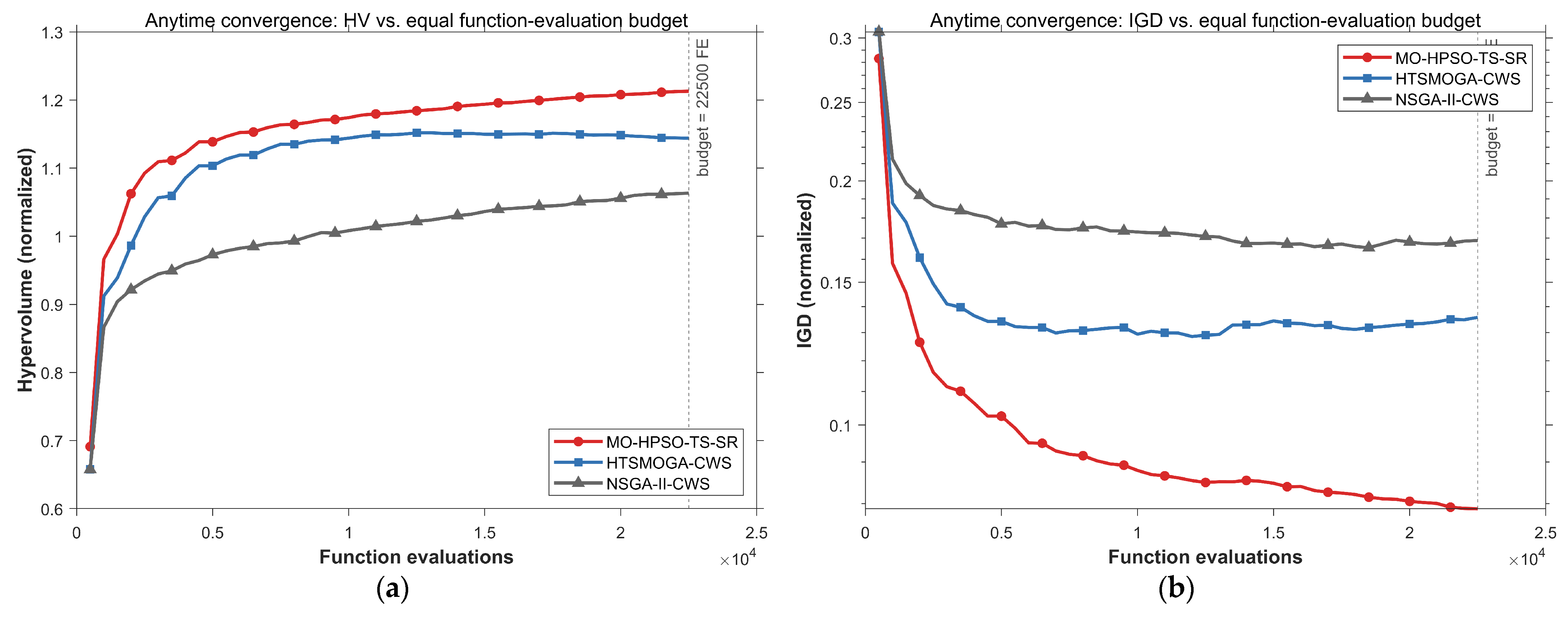
The final Pareto-front cardinality is 99.7 ± 1.1 solutions across runs, essentially saturating the archive cap of 100 with negligible run-to-run variation, indicating that the crowding-distance pruning rule of Section 2.2.6 fills the archive efficiently. The anytime convergence of the three algorithms under the equal 22,500-FE budget is shown in Figure 2, which plots the normalized hypervolume (panel a) and IGD (panel b) against the number of function evaluations. MO-HPSO-TS-SR leads both baselines at every point along the budget: it attains a higher HV and a lower IGD from the earliest evaluations onward and keeps improving through to the budget, whereas the two genetic baselines plateau earlier. The curves confirm that the ranking of the three algorithms is stable across the entire evaluation history and is therefore not an artifact of the stopping point.

3.3. Three-Algorithm Comparison on the Real Instance

Table 3 reports the three-indicator summary on the Liyang (Medium) instance under the equal-budget protocol. MO-HPSO-TS-SR achieves the best mean value on all three indicators; HTSMOGA-CWS ranks second and NSGA-II-CWS third on HV and IGD, while on SP the two genetic baselines are statistically indistinguishable (Table 4).
Pairwise statistical tests (Table 4) show that all differences are highly significant (Holm-adjusted p < 0.001 ) and of large effect size, with a single exception: HTSMOGA-CWS and NSGA-II-CWS do not differ significantly on SP ( p = 0.77 , δ = 0.060 , negligible), an early indication (developed in Section 3.4) that Tabu Search improves convergence but not distribution uniformity. The comparison MO-HPSO-TS-SR versus NSGA-II-CWS yields Cliff’s δ = + 1.000 on both HV and IGD, meaning that every one of the 20 MO-HPSO-TS-SR runs strictly dominated every one of the 20 NSGA-II-CWS runs on these two indicators, the strongest possible result on a finite sample.
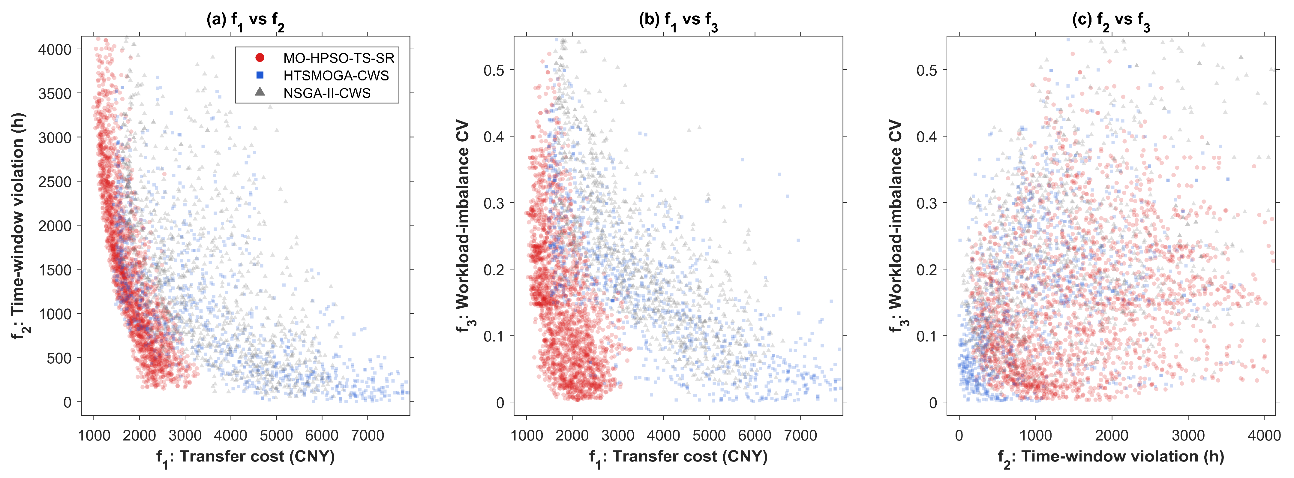
The distribution of solutions in objective space (Figure 3) shows that NSGA-II-CWS is dominated across the board, occupying the region of high transfer cost, high time-window violation, and high workload imbalance. MO-HPSO-TS-SR and HTSMOGA-CWS both advance toward the low-cost, low-imbalance corner, but with a clear division of strengths. MO-HPSO-TS-SR reaches a substantially lower transfer cost ( f 1 ) and drives the workload imbalance ( f 3 ) toward zero, whereas HTSMOGA-CWS attains a more timely extreme on f 2 . This separation reflects the workload concentration trade-off examined below.
A per-objective breakdown of the terminal fronts makes this division of strengths concrete (best, i.e., minimal, value of each objective, median over the 20 runs). On transfer cost f 1 , MO-HPSO-TS-SR reaches a median best of ≈ 1111 CNY, against ≈ 1510 CNY for HTSMOGA-CWS and ≈ 1678 CNY for NSGA-II-CWS, an economic advantage of roughly 26% over the strongest baseline and 34% over NSGA-II-CWS. On time-window violation f 2 , the ordering reverses: HTSMOGA-CWS attains the most timely solution (≈ 35 h), NSGA-II-CWS follows (≈ 118 h), and MO-HPSO-TS-SR is the least timely at its extreme (≈ 215 h). On workload imbalance f 3 , both MO-HPSO-TS-SR (≈ 0.008 ) and HTSMOGA-CWS (≈ 0.004 ) drive the coefficient of variation close to zero, whereas NSGA-II-CWS stagnates near 0.034. This pattern indicates that the Sparsity Repair operator concentrates each area’s workload onto fewer machines, sharply reducing transfer cost ( f 1 ) at a cost in time-window timeliness ( f 2 ) relative to HTSMOGA-CWS. The aggregate indicators confirm that this trade-off is strongly favorable, since MO-HPSO-TS-SR attains the best HV, IGD, and SP overall (Table 3).

3.4. Mechanism Contribution Decomposition

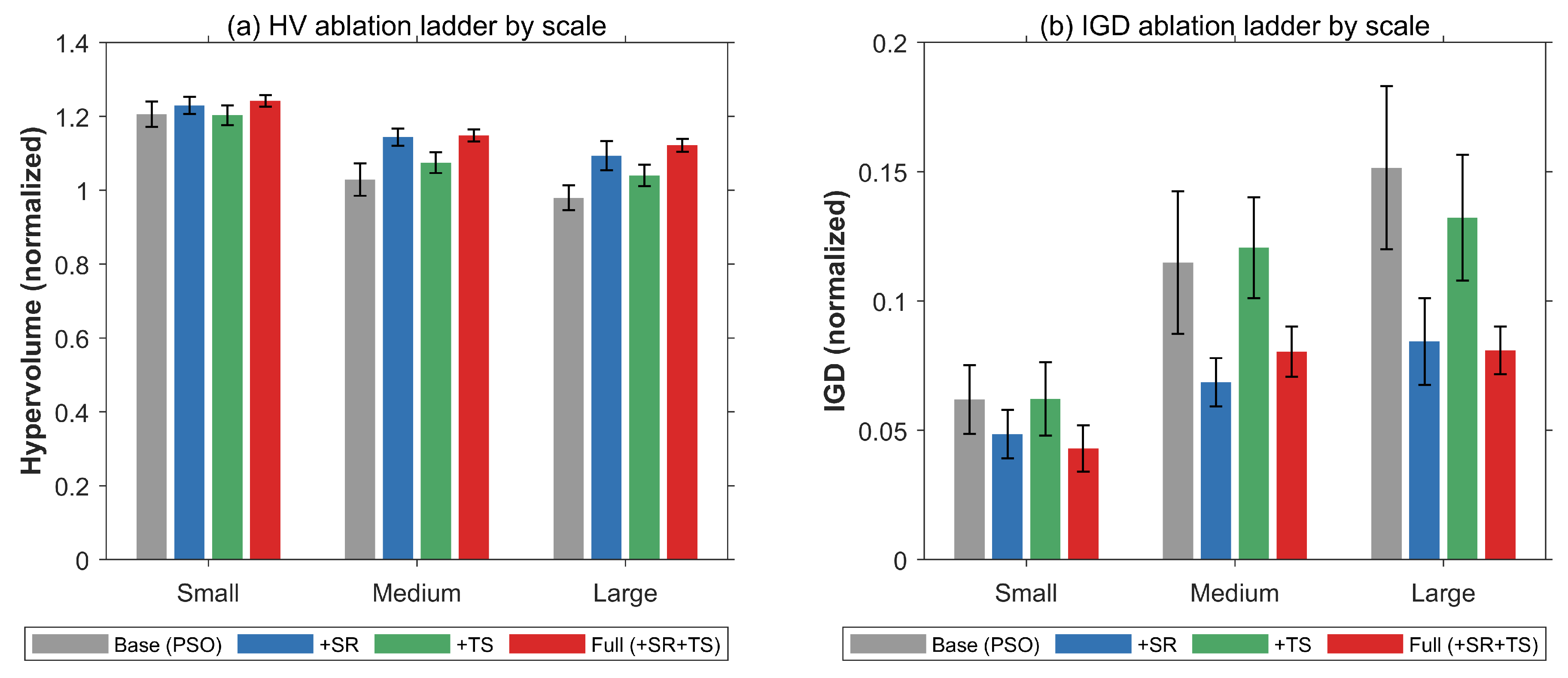
To quantify the independent contribution of each newly added module, we conduct a 2 × 2 factorial ablation that toggles Sparsity Repair (SR) and Tabu Search (TS) on and off within the PSO backbone. This yields four configurations: Base (PSO only), +SR, +TS, and Full (+SR + TS). The factorial is run on all three instances (Small, Medium, Large) under the same 22,500-FE budget, so that each module’s contribution and its dependence on problem scale can be isolated. The role of Tabu Search is then localized further, by objective and by Pareto-front region, to clarify where its refinement is most effective.
Table 5 reports the hypervolume of the four configurations at each scale, together with the drop-one contribution of each module (the HV lost when that module is removed from the Full algorithm) and the SR × TS interaction. Three findings emerge. First, Sparsity Repair is the dominant contributor, and its effect grows with problem scale: removing SR from the Full algorithm reduces HV by 0.038 (Small), 0.074 (Medium), and 0.082 (Large). On a small instance, the workload-share matrix is already close to feasible, so structural repair adds little; as the instance grows and the raw swarm output becomes increasingly sparse and ill-formed, SR’s regularization becomes essential. Second, Tabu Search contributes a smaller, scale-dependent HV gain (0.012/0.005/0.029 for Small/Medium/Large). Notably, at the Medium scale, adding TS on top of SR yields no statistically significant HV improvement (Holm-adjusted p = 0.279 ), whereas at the other two scales the Full configuration significantly exceeds all three reduced corners (Holm-adjusted p < 0.05 ). Third, the SR × TS interaction is positive on the Small instance (+0.015) but negative on the Medium (−0.041) and Large (−0.032) instances, indicating that on larger problems the two modules partially overlap in the gains they deliver rather than compounding. The inverted generational distance (Figure 4b) reinforces this picture: SR sharply reduces IGD at every scale, whereas TS alone barely moves it, and on the Medium instance, adding TS on top of SR even raises IGD (0.069→0.081), an early sign, examined next, that TS reallocates search effort away from broad front coverage. Figure 4 visualizes the full ablation ladder.
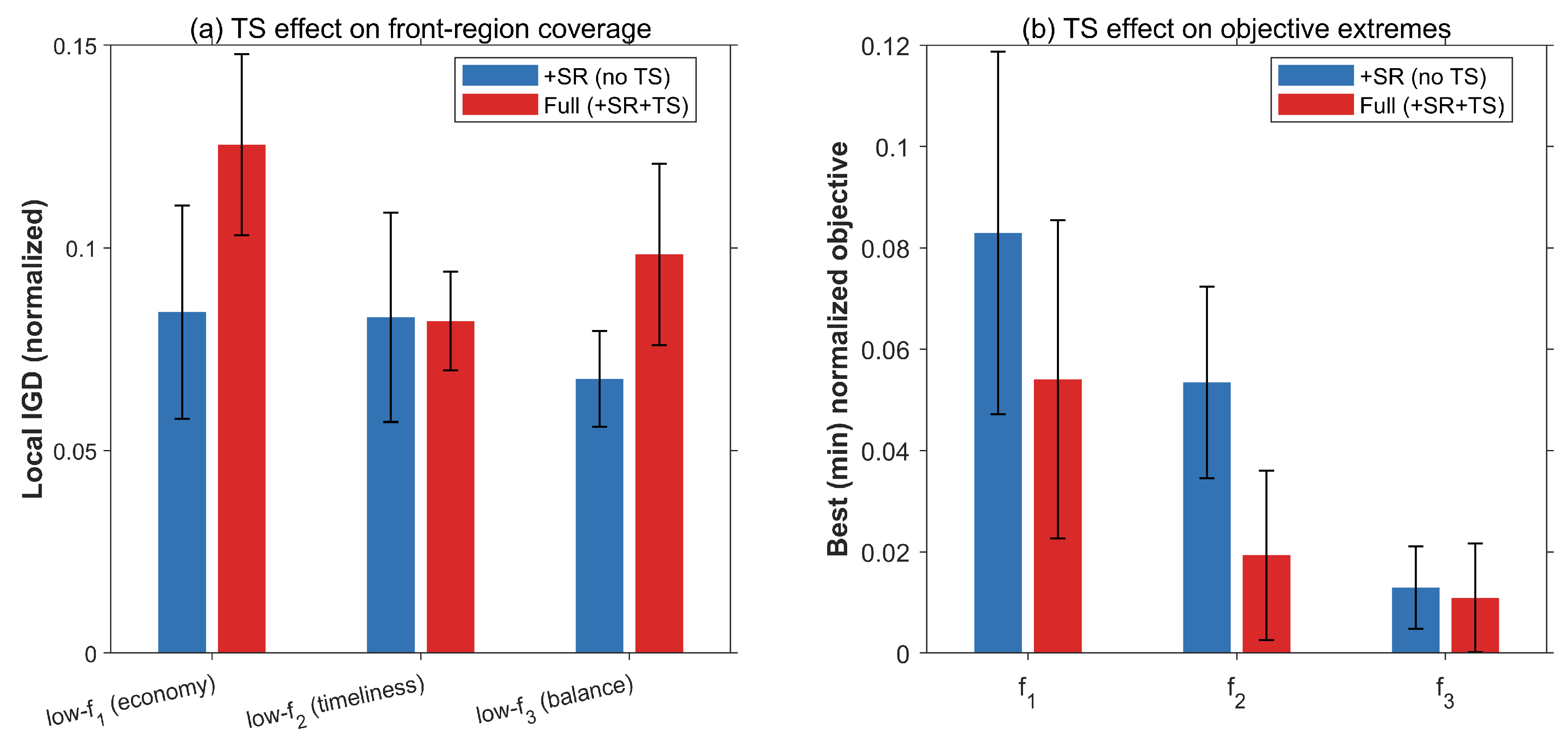
Why does Tabu Search contribute so modestly to the aggregate indicators, and even degrade IGD in some settings? A region- and objective-resolved analysis on the Medium instance (Figure 5) provides the answer: TS does not broaden coverage of the front; it sharpens its extremes. Partitioning the front into an economy region (low f 1 ), a timeliness region (low f 2 ), and a balance region (low f 3 ), the local IGD within each region (Figure 5a) shows that adding TS leaves the low f 2 region essentially unchanged (+1%, p = 0.74 ) but thins coverage (raising local IGD) in the low f 1 region (−49%, Holm-adjusted p < 0.001 ) and the low f 3 region (−45%, Holm-adjusted p < 0.0 1). At the same time, TS markedly extends the single-objective extremes (Figure 5b). It drives the best attainable f 1 a further 35% lower (Holm-adjusted p = 0.016 ) and the best attainable f 2 a further 64% lower (Holm-adjusted p < 0.001 ), with no significant change to the best f 3 ( p = 0.16 ). Tabu Search thus redirects effort from filling the middle of the front toward pushing the economy and timeliness tips further out, a desirable behavior for a decision-support tool, since it supplies cooperative managers with more extreme low-cost and high-timeliness options at a modest cost in mid-front density that Sparsity Repair and the diversity-preserving archive already secure.
Taken together, the two analyses give a clear division of labor. Sparsity Repair is the principal engine of aggregate front quality (its contribution to both HV and IGD grows with problem scale), while Tabu Search plays a complementary, targeted role, extending the extreme economy and timeliness solutions rather than thickening the front. The two mechanisms are therefore complementary rather than redundant, which is why the Full configuration is retained despite the negative SR × TS interaction on the larger instances.

3.5. Multi-Scale Generality Validation

To verify that the advantage of MO-HPSO-TS-SR is intrinsic to the algorithm rather than an artifact of the specific Liyang instance, the three-algorithm comparison was repeated on the three synthetic scales defined in Section 3.1.1. Each algorithm was run 20 times per scale under the identical 22,500-FE budget and hyperparameters of Table 2, and a unified composite reference front was constructed separately for each scale to keep the normalization unbiased. The Medium scale corresponds to the Liyang instance, so its row reproduces the values reported in Table 3 exactly. Table 6 summarizes the three-indicator performance of all three algorithms at each of the three scales.
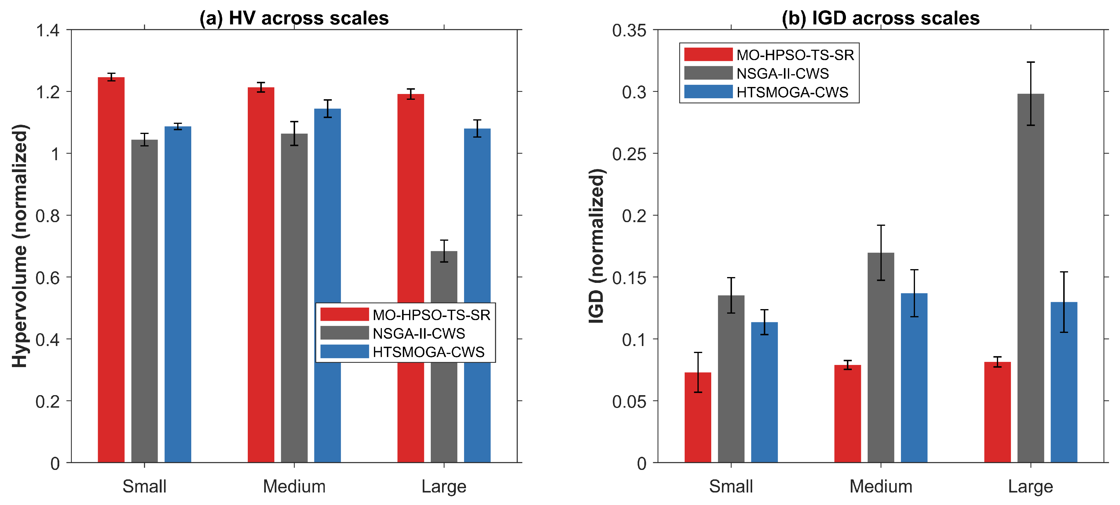
Across all three scales, MO-HPSO-TS-SR attains the best mean value on every indicator, in nine of nine metric-scale combinations (Table 6, Figure 6). The dominance is statistically decisive: on the primary indicators HV and IGD, every comparison against both baselines is significant after Holm correction (Holm-adjusted p = 1.8 × 10 4 ; raw paired Wilcoxon signed-rank p = 8.9 × 10 5 ), with Cliff’s δ = + 1.0 in ten of the twelve HV/IGD comparisons and δ + 0.975 in all twelve. On the spacing indicator, the margin is also significant at every scale (Holm-adjusted p 6 × 10 3 ).
The relative-advantage pattern differs sharply between the two baselines. Against NSGA-II-CWS, the margin is moderate on the smaller instances, a 19.4% (Small) and 14.0% (Medium) HV lead, but widens dramatically to 74.2% on the Large instance; the IGD reduction tells the same story, growing monotonically from 46.0% to 53.4% to 72.7%. This widening is driven by the collapse of NSGA-II-CWS itself: from the Small to the Large instance, its mean HV falls by 34.5% (1.044 → 0.684) and its IGD more than doubles (0.135→0.298), reflecting its lack of any mechanism to regularize the increasingly sparse, high-dimensional workload-share matrix, consistent with the growing importance of Sparsity Repair documented in Section 3.4. Against the stronger HTSMOGA-CWS baseline, by contrast, the HV advantage is smaller and approximately scale-invariant (14.7%, 6.0%, 10.3%), and the IGD reduction stays within a narrow band (35.7%, 42.4%, 37.3%). This is because HTSMOGA-CWS shares the Tabu Search component and therefore degrades only mildly with scale (HV −0.6% from Small to Large). Two conclusions follow. First, the complete MO-HPSO-TS-SR architecture scales markedly better than a plain genetic backbone on larger, higher-dimensional instances. Second, the incremental value of the PSO update kernel, Sparsity Repair, and the external archive over a Tabu-Search-equipped genetic baseline is consistent across scales rather than vanishing or exploding with problem size.
Run-to-run stability remains strong throughout. The HV coefficient of variation of MO-HPSO-TS-SR stays at or below 1.4% across all scales (1.0%, 1.3%, 1.4% from Small to Large), the lowest of the three algorithms at the Medium and Large scales and within 0.03 percentage points of the best at the Small scale. Its solution spacing is the tightest at every scale, even improving from 0.0228 to 0.0168 as the instance grows. The external archive thus keeps both convergence and distribution within a narrow band as the decision space expands, whereas the genetic baselines show markedly larger dispersion at the Large scale (HV CV up to 5.2% for NSGA-II-CWS).
Finally, because the external archive lets MO-HPSO-TS-SR return roughly twice as many solutions (≈100) as the 50-member genetic baselines, we verified that its advantage is not an artifact of front cardinality. Truncating each MO-HPSO-TS-SR front to 50 solutions by crowding distance barely changes its indicators (mean HV down by at most 0.3%, mean IGD up by at most 9% at every scale), and the truncated method still attains the best HV and IGD at all three scales, with margins essentially identical to the full-front values in Table 6 and all twelve HV/IGD comparisons remaining significant after Holm correction. The performance gap is therefore intrinsic to the quality of the front approximation, not a consequence of returning more points.

3.6. Computational Cost

Because all three algorithms were executed under the same 22,500 function-evaluation budget (Section 3.1.2), their wall-clock times reflect per-evaluation efficiency rather than any difference in computational allowance. Table 7 reports the mean per-run runtime at each scale. MO-HPSO-TS-SR is the fastest of the three at every scale. It needs roughly half the time of either genetic baseline on the Small instance (7.4 s versus 15.3 s for NSGA-II-CWS and 14.5 s for HTSMOGA-CWS) and remains the quickest on the Large instance (29.7 s versus 32.1 s and 38.1 s). The advantage narrows as the instance grows because objective evaluation, common to all methods, comes to dominate the per-iteration cost. On the smaller instances, where evaluation is cheap, the per-generation overhead of non-dominated sorting and genetic recombination makes the two GA-based baselines comparatively more expensive. NSGA-II-CWS, in particular, must run additional generations to consume the same budget that the Tabu-Search-equipped methods spend partly on local search.
Because MAMSP-CWS is solved offline during pre-season planning, runtime differences of this magnitude (tens of seconds) carry no operational significance. One cost-related distinction is nonetheless worth recording: by virtue of its external archive of capacity 100, MO-HPSO-TS-SR returns roughly twice as many Pareto-optimal solutions per run as either genetic baseline (≈98 versus 50). It therefore not only runs fastest but also delivers the lowest cost per Pareto solution of the three methods, furnishing the dispatcher with a substantially denser approximation of the trade-off surface for the same (indeed, lower) computational effort.

3.7. Route-Order Sensitivity

The decoder visits each tractor’s assigned areas in time-window order, sorted by the window lower bound a i (Section 2.1), rather than optimizing the visit sequence for distance. Because the transfer cost f 1 depends on the visit order, it is important to verify that fixing this order does not bias the objectives. To this end, every terminal Pareto solution of every algorithm was post-processed. Holding the area-to-tractor assignment and the workloads fixed, each tractor’s visit sequence was re-optimized by 2-opt to minimize transfer distance, and f 1 and f 2 were recomputed under the same waiting-allowed model. The workload-balance objective f 3 depends only on per-cooperative totals and is invariant to visit order.
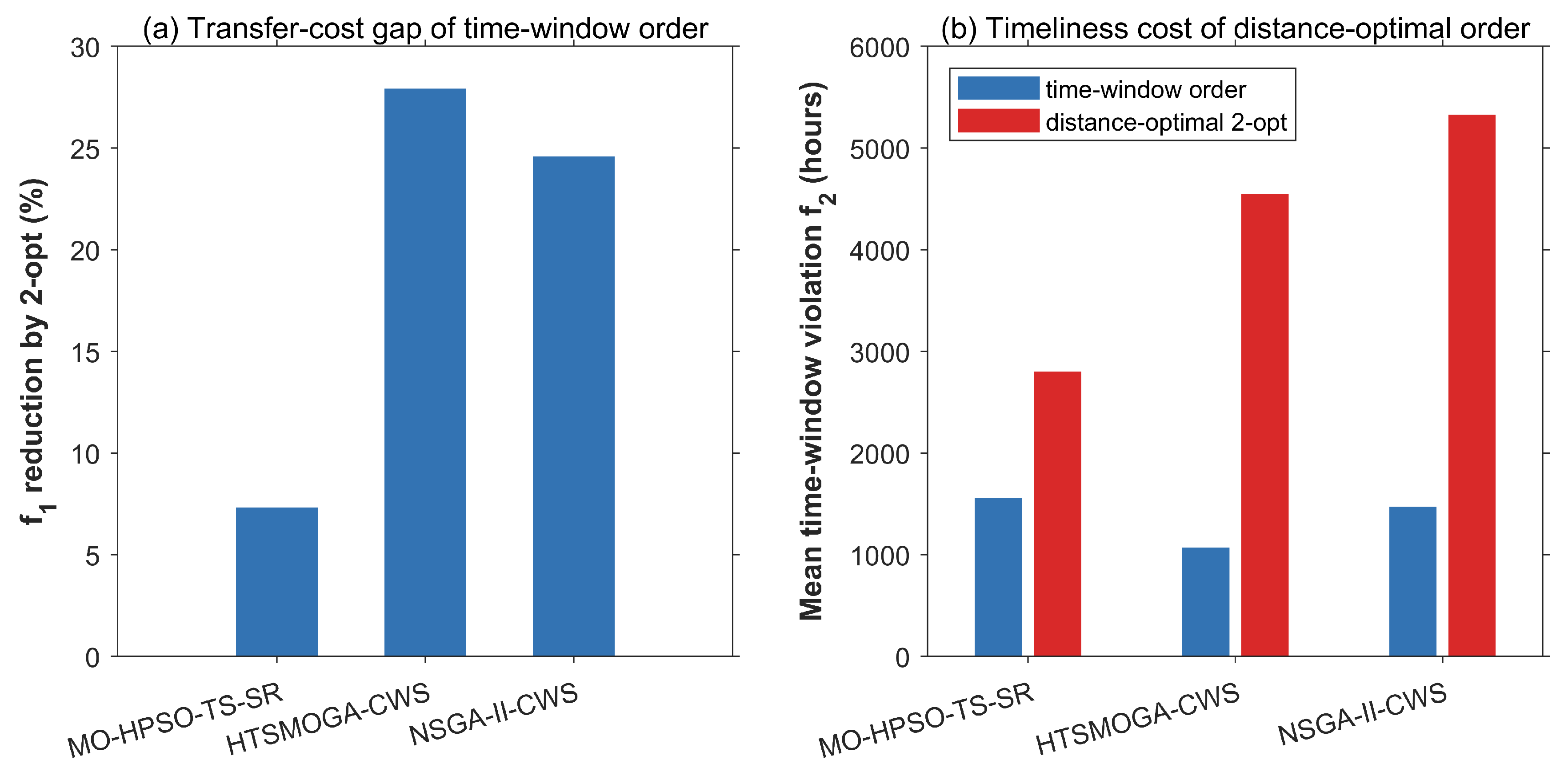
The result is a clear timeliness-for-efficiency trade-off (Figure 7). Distance-optimal re-ordering does reduce transfer cost by 7.3% for MO-HPSO-TS-SR and by roughly 25–28% for the two genetic baselines (24.6% for NSGA-II-CWS, 27.9% for HTSMOGA-CWS). However, this comes at a steep cost in timeliness: the mean time-window violation of MO-HPSO-TS-SR rises from 1554 h to 2801 h (a 1.8-fold increase), and that of the baselines increases 3.6- to 4.2-fold (HTSMOGA-CWS 1072 h → 4549 h; NSGA-II-CWS 1469 h → 5326 h), with 99–100% of all solutions becoming worse on f 2 . The time-window visit order is therefore a deliberate choice that sacrifices a modest amount of transfer efficiency to protect timeliness, not an oversight that biases the reported objectives. The markedly smaller transfer-cost slack of MO-HPSO-TS-SR (7.3% versus ~25%) further indicates that its solutions already approach distance efficiency while honoring the time-window structure. Together with the waiting-allowed dispatch rule introduced in Section 2.1, this analysis confirms the realism of the scheduling sub-model: neither the no-early-start rule nor the time-window visit order distorts the Pareto fronts reported above.

3.8. Fairness of the Workload-Balance Objective

The third objective measures cross-cooperative equity through the coefficient of variation (CV) of the per-tractor workload across cooperatives (Section 2.1). Two questions motivate a closer look: whether this workload-based CV adequately captures fairness in the time dimension, and whether the CV is the most appropriate inequality measure. Both are examined on the Liyang instance over the full set of 1993 terminal Pareto solutions found across the 20 runs.
First, under the model’s homogeneous-efficiency assumption, workload fairness and time fairness coincide exactly. Each cooperative’s per-tractor working hours equal its per-tractor workload divided by a common efficiency η , and because the CV is scale-invariant, the CV of per-tractor hours equals the CV of per-tractor workload (and therefore f 3 ) to machine precision (maximum discrepancy 2 × 10 16 across all 1993 solutions). The workload-balance objective is thus already a time-fairness measure: equalizing per-tractor workloads across cooperatives equalizes their per-tractor working hours.
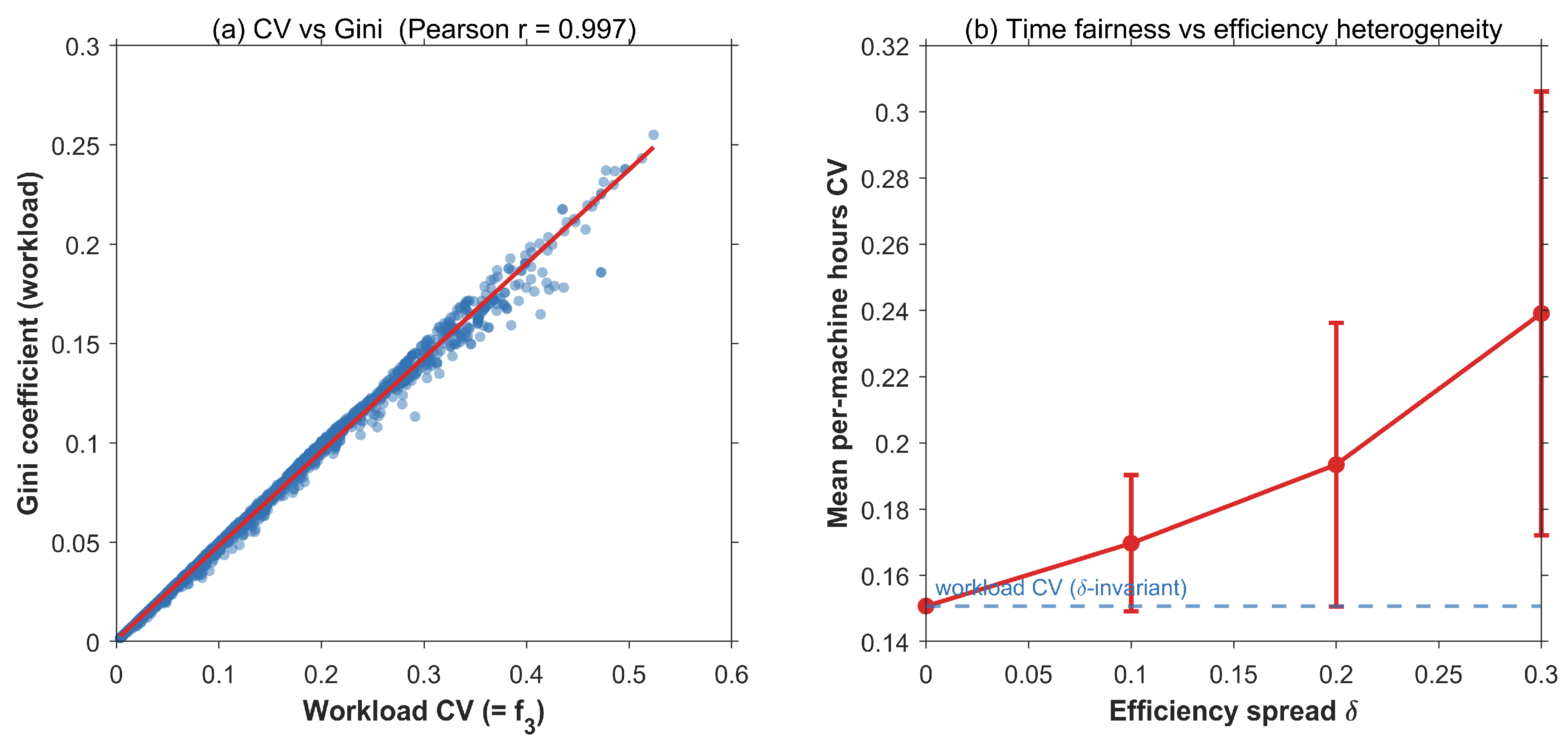
Second, the CV ranks fairness almost identically to the Gini coefficient, the canonical inequality index: across the terminal solutions, the two are correlated at r = 0.997 (Pearson) and ρ = 0.999 (Spearman) (Figure 8a). The CV is preferred here because it is dimensionless, mean-relative, and symmetric, and because it enters the gradient-free search directly as a smooth scalar objective.
Third, the equivalence between workload and time fairness is specific to the homogeneous-fleet assumption. When cooperative efficiencies are drawn with increasing heterogeneity ( η c = η 0 1 + δ U 1 ,   1 , the mean per-tractor-hours CV departs upward from the workload CV, from 0.151 at δ = 0 to 0.170, 0.193, and 0.239 at δ = 0.1 , 0.2, and 0.3 (Figure 8b), because equal workloads no longer imply equal hours. This delimits the regime in which a dedicated time-fairness objective would be warranted and motivates the heterogeneous-fleet extension discussed in Section 4.

4. Discussion

The empirical evaluation in Section 3 establishes that MO-HPSO-TS-SR dominates two well-designed baselines on the MAMSP-CWS problem across multiple instance scales. This section interprets those findings and situates them within the broader literature. We first benchmark the results against prior and related work, showing that the advantage stems from the algorithm rather than from the problem encoding (Section 4.1). We then examine two patterns in the data that carry implications beyond the present application. The first is a sparsity-for-timeliness trade-off intrinsic to multi-machine cooperative scheduling, here rendered explicit and quantifiable (Section 4.2). The second is the robustness of solution quality to problem scale, whose mechanism we trace to the interplay of Sparsity Repair and local search (Section 4.3). Finally, we discuss the practical implications for cooperative management (Section 4.4) and the limitations of the present study (Section 4.5).

4.1. Comparison with Prior and Related Work

The present results both confirm and extend the cooperative-scheduling literature. Relative to our single-objective predecessor [2], which optimized a weighted sum of transfer cost, earliness, and tardiness, the three-objective formulation recovers the same qualitative sparsity-for-timeliness behavior but renders it explicit and navigable: the marginal exchange rate between transfer cost and timeliness (fixed a priori by the weight in [2]) is now read directly off the Pareto front (Section 3.3, Figure 3), and the contribution of the Sparsity Repair operator is isolated for the first time (Section 3.4) rather than confounded within an aggregate score.
Crucially, we did not compare across studies that adopt incompatible problem encodings (discrete area-to-machine assignment [8,12], permutation-based field routing [7,19], or clustering-then-assignment pipelines [13]). Instead, we benchmarked the proposed method against faithful re-implementations of the two dominant multi-objective paradigms on the identical Continuous Workload Sharing representation: the elitist non-dominated-sorting genetic algorithm NSGA-II [22], the de facto standard for multi-objective combinatorial problems [23], and the Tabu-Search-hybridized multi-objective genetic algorithm of Guo et al. [3], the leading hybrid for cross-regional agricultural scheduling with time windows. On this controlled footing, MO-HPSO-TS-SR dominates both baselines across all three indicators and all three instance scales (Section 3.3 and Section 3.5), establishing that the advantage stems from the algorithm itself rather than from differences in problem representation.
These findings align with the broader evidence that hybrid metaheuristics outperform single-paradigm search on agricultural scheduling (whether NSGA-II combined with simulated annealing [1], NSGA-III augmented with biology-based or ant-colony search [4,8], or genetic-ant-colony hybrids [18]) and with the memetic-computing principle that intensive local refinement accelerates the convergence of population-based optimizers on scheduling problems [39,40]. They also corroborate the specific observation of Guo et al. [3] that intermittent Tabu-Search refinement sharpens convergence; here the same mechanism is shown (Section 3.4) to act primarily on the extremes of the Pareto front. The distinctive advance is the pairing of this hybrid search with the CWS encoding and the Sparsity Repair operator, which together resolve a structural pathology (the accumulation of operationally meaningless fractional assignments) that discrete-assignment formulations [8,12] never encounter and therefore provide no mechanism to address.
Beyond agriculture, the architecture (a continuous-share encoding, an external Pareto archive with crowding-based pruning, and local-search intensification) targets the general class of resource-pooling, multi-objective scheduling problems; multi-objective particle-swarm variants have likewise proven effective in adjacent domains such as energy-storage configuration with electric-vehicle dispatch [33] and energy-efficient distributed flow-shop scheduling [41]. The same continuous, gradient-free formulation extends naturally to multi-parameter joint optimization in process-systems engineering, where coupled operating variables must be balanced against competing performance criteria [47].

4.2. The Sparsity-for-Timeliness Trade-Off

The per-objective breakdown in Section 3.3 exposes a paradoxical relationship between assignment density and objective performance. HTSMOGA-CWS, which omits Sparsity Repair, produces structurally denser assignment matrices and reaches the single most timely solution at its best-timeliness corner (ahead of both NSGA-II-CWS and MO-HPSO-TS-SR on that one extreme), which, viewed in isolation, would seem to recommend dense assignment. That density is costly elsewhere, however. MO-HPSO-TS-SR’s median-best transfer cost lies 26% below HTSMOGA-CWS and 34% below NSGA-II-CWS, and it attains the best hypervolume, IGD, and spacing overall. Both the SR-equipped and the non-SR variants hold workload imbalance well below NSGA-II-CWS, which stagnates near 0.034 (Section 3.3). Sparsity Repair, by concentrating each area’s workload onto the minimum tractor count its time window permits, reshapes the achievable frontier toward economy. It concedes the best-timeliness corner in exchange for a large transfer-cost reduction and a dominant overall front, while sacrificing nothing on the equity axis.
A second design lever, the time-window visit order, pulls in the opposite direction and actively protects timeliness. The route-order analysis of Section 3.7 shows that re-optimizing each tractor’s visit sequence purely for distance lowers transfer cost but inflates time-window violation by factors of 1.8 to 4.2 across the three algorithms; the decoder’s time-window ordering therefore gives up a little efficiency to safeguard timeliness, the mirror image of the density trade. Across the knee region of the Pareto front, moreover, the marginal cost of buying additional timeliness is roughly an order of magnitude below the average cost-per-hour that a fixed-weight objective would impose. A planner navigating the front, therefore, pays far less for timeliness at the margin than a single weighted score would suggest.
This trade-off is not normatively settled. For harvesting operations bound by strict pre-purchase commitments, where a missed window can forfeit the sale, the dense, timeliness-minimizing region of the front may be the rational choice. For routine field operations with flexible windows, the sparse, cost-minimizing region is preferable.

4.3. Mechanisms of Robustness to Problem Scale

The cross-scale validation in Section 3.5 shows that MO-HPSO-TS-SR’s hypervolume advantage over NSGA-II-CWS widens with problem size, although non-monotonically. This widening is driven not by a growing advantage of the proposed mechanisms but by the disproportionate degradation of NSGA-II-CWS itself, whose absolute hypervolume collapses across scales while MO-HPSO-TS-SR and HTSMOGA-CWS barely degrade; all pairwise gaps nonetheless remain significant at every scale (Section 3.5). Because conventional expectation in evolutionary computation anticipates the opposite (that an algorithm strong on small instances will lose ground as dimensionality grows and the search space becomes harder to traverse), the widening margin warrants a mechanistic rather than a purely empirical reading.
Two complementary analyses localize the cause and together correct a tempting but incomplete explanation. Within the genetic family, Tabu Search is what averts collapse: HTSMOGA-CWS, which augments the same genetic backbone as NSGA-II-CWS with Tabu Search but contains no Sparsity Repair, remains almost perfectly scale-robust, so focused local-search intensification rescues a population that the global evolutionary operators alone increasingly fail to refine as the Continuous Workload Sharing decision space expands. It would be wrong, however, to conclude that local search alone confers robustness: the ablation within the proposed particle-swarm backbone (Section 3.4) shows that Sparsity Repair, not Tabu Search, is the dominant contributor to MO-HPSO-TS-SR’s quality, with its marginal contribution growing as the problem scales while Tabu Search remains secondary. The two findings reconcile once robustness is seen as backbone-dependent: in a plain genetic backbone, local search is the decisive rescue, whereas in the proposed method, Sparsity Repair is the primary regularizer of the increasingly sparse, high-dimensional workload-share matrix, with Tabu Search a complementary refiner of the front’s extremes. NSGA-II-CWS collapses because it carries neither a sparsity-regularizing operator nor local-search intensification; MO-HPSO-TS-SR resists scale because it carries both.
This dual protection also explains the residual gap between the two hybrids: MO-HPSO-TS-SR’s advantage over the Tabu-Search-equipped HTSMOGA-CWS is modest and non-monotonic (Section 3.5), indicating that the incremental value of the particle-swarm kernel, Sparsity Repair, and the external archive over a strong hybrid baseline persists across scales rather than eroding. The practical implication is favorable: cooperative networks that expand over time to incorporate additional fields or member organizations retain the full benefit of the proposed algorithm, because its solution quality is safeguarded by two independent mechanisms (sparsity regularization and local-search intensification) rather than by either one alone.

4.4. Practical Implications for Cooperative Management

Beyond its algorithmic properties, the multi-objective Pareto-front representation supplies cooperative dispatchers with a fundamentally richer decision artifact than a single optimized schedule. The front produced by MO-HPSO-TS-SR (up to roughly one hundred non-dominated plans, the external-archive capacity; Section 3.5) is a navigable surface in the three-dimensional cost-time-equity space, on which a coordinator can locate regions of acceptable performance and choose among them according to priorities that shift seasonally, contractually, or with the weather. A coordinator facing an imminent rainfall forecast may move to the low-f2 (most timely) corner; one managing inter-cooperative grievances may move to the low-f3 (most equitable) corner; in routine conditions, the knee region offers the most balanced compromise. The output thus reframes dispatching from a one-shot optimization into a decision-support workflow in which the algorithm delimits the set of rational compromises rather than dictating a single answer.
Integrating the method is undemanding because it consumes only data a federation already maintains or can readily assemble: each cooperative’s fleet roster, geo-referenced work areas with workloads, the agronomic time window of each area, a transfer-cost rate per unit distance, and a representative machine work rate. From these inputs, the solver returns the full Pareto set in under a minute even at the Large scale (Section 3.6), so it can run on demand within a dispatch dashboard, with the coordinator inspecting the surface, committing to a plan, and re-running whenever fields ripen, machines free up, or forecasts change. Each row of the resulting workload-share matrix maps directly to a tractor’s per-machine work order, with visits ordered by time window, so the algorithm serves as a continuous planning aid that leaves the final, context-dependent decision to the human coordinator.

4.5. Limitations and Threats to Validity

The model abstracts several features of real field operations, each defining an avenue for refinement. The fleet is assumed homogeneous (Assumption 1, Section 2.1.1): every tractor shares a single work efficiency η and travel speed ν , whereas larger cooperatives operate machines of different capacities and speeds. Section 3.8 quantifies one consequence of relaxing this assumption: as efficiency heterogeneity grows, per-tractor working-hour fairness departs upward from workload fairness, the per-tractor-hour coefficient of variation rising from 0.151 to 0.239 as the spread widens. A genuinely heterogeneous fleet would therefore warrant per-tractor parameters ( η m , ν m ) and a dedicated time-fairness objective, an extension that enlarges the model without altering its structure. The routing model further assumes that each tractor begins and ends at its depot (Assumption 2, Section 2.1.1) and measures inter-area movement by great-circle (Haversine) distance, which approximates rather than reproduces travel on the actual road network. By contrast, the earlier serve-on-arrival idealization has already been relaxed: the waiting-allowed rule of Section 2.1 lets a machine idle until a window opens at no charge, removing a distortion of the economy–timeliness trade-off.
More broadly, the formulation is deterministic. Time windows and travel times are treated as fixed and known, whereas peak-season operations are subject to weather-induced shifts in field readiness, machine breakdowns, operator shift and working-hour limits, refueling and resupply stops, and variable road conditions. Each of these introduces uncertainty or mid-season disruption that a single static plan cannot anticipate. The fast solve time (Section 3.6) already supports rolling re-optimization as conditions evolve (Section 4.4), but explicitly representing these factors (through a stochastic or robust formulation, chance-constrained time windows, or dynamic rescheduling) would capture operational reality more faithfully.
Finally, although the evaluation spans a 24-fold range of decision-space sizes, all instances are calibrated to a single geographic source (the Liyang dataset and the empirical distributions sampled from it), so cooperatives with different field-size distributions, time-window densities, or transport infrastructure may exhibit additional regime-dependent behavior, and validation across diverse regions remains valuable. These limitations, and the extensions they motivate, are taken up in Section 5.

5. Conclusions

5.1. Summary of Contributions

This paper formulated multi-cooperative agricultural machinery scheduling under continuous workload sharing (MAMSP-CWS) as a three-objective optimization problem, minimizing transfer cost, time-window violation, and cross-cooperative workload imbalance, and proposed MO-HPSO-TS-SR, a hybrid that combines particle swarm optimization, tabu search, and an external Pareto archive with the Sparsity Repair operator from our prior single-objective study [2]. The Continuous Workload Sharing encoding and Sparsity Repair are carried over from [2]; the three-objective formulation, the multi-objective hybrid architecture, and the re-analysis of Sparsity Repair as a structural regularizer of the high-dimensional workload-share matrix are new to this work.
Evaluated against NSGA-II-CWS and an HTSMOGA-CWS adaptation of Guo et al. [3] over 20 independent runs at each of three scales, MO-HPSO-TS-SR attained the best mean value on every metric-by-scale combination, with a decisive convergence advantage on hypervolume and IGD and a favorable spacing margin (Section 3.3, Section 3.4 and Section 3.5). A mechanism-level decomposition identified Sparsity Repair as the dominant contributor to convergence quality and Tabu Search as a complementary refiner of the front’s extremes, and showed the algorithm’s scale-robustness to be backbone-dependent (Section 3.4): its relative advantage over a plain genetic baseline grows with problem size, driven by that baseline’s disproportionate collapse rather than by a growing advantage of the proposed mechanisms. The archive-based design additionally returns roughly twice the Pareto-front cardinality of the (P + Q)-based baselines, furnishing decision-makers with a denser approximation of the trade-off surface at comparable computational cost.

5.2. Future Work

The limitations identified in Section 4.5 motivate several natural extensions of the present study.
First, the deterministic time-window assumption can be relaxed by embedding the proposed algorithm within a stochastic or robust-optimization framework, in which weather-induced time-window shifts are modeled as probability distributions or uncertainty sets. The Pareto-front structure exposed by the multi-objective formulation should facilitate such extension, since robustness can be introduced either as a fourth objective or as a chance-constraint refinement of the existing constraints.
Second, the homogeneous-fleet assumption can be relaxed by introducing per-tractor efficiency and travel-speed parameters η m and v m , expanding the model to accommodate the heterogeneous machinery found in larger cooperative networks (e.g., wheeled vs. tracked harvesters). This extension preserves the CWS encoding and the algorithm structure intact; only the decoder of Section 2.1.3 requires modification.
Third, the present single-day formulation can be extended to multi-day campaign planning, in which tractor positions at the end of one day’s schedule become the starting positions of the next, and depot returns become optional. Such an extension would couple successive scheduling instances and may favor algorithms with explicit cross-day archival, an avenue for which the external-archive mechanism developed here provides a natural foundation.
Beyond these direct extensions, an open question concerns whether the Sparsity Repair operator generalizes to other continuous-encoding combinatorial domains (vehicle routing with flexible service shares, multi-machine job-shop scheduling, or warehouse-task assignment) where similar density-induced inefficiencies may arise. A systematic investigation of this transferability is left to future work.

Supplementary Materials

The following supporting information can be downloaded at: https://www.mdpi.com/article/10.3390/pr14132181/s1, MATLAB source code for the proposed MO-HPSO-TS-SR algorithm and baselines; MATLAB data files containing all experimental results; The empirical dataset of the Liyang instance (DATA_LIYANG.xlsx).

Author Contributions

Conceptualization, W.W. and Q.J.; methodology, W.W.; software, W.W.; validation, W.W., S.Q., J.C. and Q.J.; formal analysis, W.W.; investigation, W.W., S.Q. and Q.J.; resources, J.C. and Q.J.; data curation, J.C. and Q.J.; writing—original draft preparation, W.W.; writing—review and editing, Q.J.; visualization, W.W.; supervision, Q.J.; project administration, W.W.; funding acquisition, Q.J. All authors have read and agreed to the published version of the manuscript.

Funding

This research was funded by the Open Project of the Key Laboratory of Modern Agricultural Equipment, Ministry of Agriculture and Rural Affairs, China (Grant No. 2023012); the Philosophy and Social Science Research Project of Jiangsu Higher Education Institutions (Grant No. 2021SJA0453); the Agricultural Science and Technology Innovation Program (Grant No. CAAS-ZDRW202506); and the Basic Research Center, Innovation Program of Chinese Academy of Agricultural Sciences (CAAS-BRC-SAE-2025-01).

Data Availability Statement

The original contributions presented in this study are included in the Supplementary Materials. Further inquiries can be directed to the corresponding author.

Conflicts of Interest

The authors declare no conflicts of interest.

References

  1. Liu, H.; Luo, J.; Zhang, L.; Wang, F.; Wang, S. Optimal Scheduling of Agricultural Machines in Hilly Mountainous Areas Based on NSGA-II-SA Hybrid Algorithm with Applications. Int. J. Agric. Biol. Eng. 2025, 18, 234–245. [Google Scholar] [CrossRef]
  2. Wang, W.; Tu, Y.; Wang, Y.; Jiang, Q. Multi-Cooperative Agricultural Machinery Scheduling with Continuous Workload Allocation: A Hybrid PSO Approach with Sparsity Repair. Agriculture 2026, 16, 136. [Google Scholar] [CrossRef]
  3. Guo, Y.; Zhang, F.; Chang, S.; Li, Z.; Li, Z. Research on a multiobjective cooperative operation scheduling method for agricultural machinery across regions with time windows. Comput. Electron. Agric. 2024, 224, 109121. [Google Scholar] [CrossRef]
  4. Yang, M.; Chen, Y.; Li, Y.; Zhang, T.; Wu, T. A Two-Stage Hybrid NSGA-III with BWO for Path Planning and Task Allocation in Agricultural Land Preparation. PLoS ONE 2025, 20, e0315670. [Google Scholar] [CrossRef] [PubMed]
  5. Wang, Z.; Zhang, F.; Ma, S.; Wang, H.; Zhang, S.; Gao, X. Research on Collaborative Scheduling Strategies of Multi-Agent Agricultural Machinery Groups. Sci. Rep. 2025, 15, 9045. [Google Scholar] [CrossRef] [PubMed]
  6. Bochtis, D.D.; Sørensen, C.G.; Busato, P. Advances in Agricultural Machinery Management: A Review. Biosyst. Eng. 2014, 126, 69–81. [Google Scholar] [CrossRef]
  7. Seyyedhasani, H.; Dvorak, J.S. Using the Vehicle Routing Problem to Reduce Field Completion Times with Multiple Machines. Comput. Electron. Agric. 2017, 134, 142–150. [Google Scholar] [CrossRef]
  8. Li, S.; Zhang, M.; Wang, N.; Cao, R.; Zhang, Z.; Ji, Y.; Li, H.; Wang, H. Intelligent Scheduling Method for Multi-Machine Cooperative Operation Based on NSGA-III and Improved Ant Colony Algorithm. Comput. Electron. Agric. 2023, 204, 107532. [Google Scholar]
  9. Cao, R.; Li, S.; Ji, Y.; Zhang, Z.; Xu, H.; Zhang, M.; Li, M.; Li, H. Task Assignment of Multiple Agricultural Machinery Cooperation Based on Improved Ant Colony Algorithm. Comput. Electron. Agric. 2021, 182, 105993. [Google Scholar] [CrossRef]
  10. Bochtis, D.D.; Sørensen, C.G. The Vehicle Routing Problem in Field Logistics: Part II. Biosyst. Eng. 2010, 105, 180–188. [Google Scholar] [CrossRef]
  11. Bochtis, D.D.; Sørensen, C.G. The Vehicle Routing Problem in Field Logistics: Part I. Biosyst. Eng. 2009, 104, 447–457. [Google Scholar] [CrossRef]
  12. Wang, Y.-J.; Huang, G.Q. A Two-Step Framework for Dispatching Shared Agricultural Machinery with Time Windows. Comput. Electron. Agric. 2022, 192, 106607. [Google Scholar] [CrossRef]
  13. Jia, L.; Zhang, Q.; Liu, S.; Kong, B.; Liu, Y. Multi-Station Agricultural Machinery Scheduling Based on Spatiotemporal Clustering and Learnable Multi-Objective Evolutionary Algorithm. AgriEngineering 2025, 7, 197. [Google Scholar] [CrossRef]
  14. Liu, H.Y.; Luo, J.H.; Zhang, L.H.; Yu, H.; Zou, S.; Wang, S. Cooperative Scheduling Method for Harvester and Grain Transport Vehicle Based on IMPA Algorithm. Int. J. Agric. Biol. Eng. 2026, 19, 226–240. [Google Scholar] [CrossRef]
  15. Wang, N.; Li, S.D.; Xiao, J.X.; Wang, T.H.; Han, Y.X.; Wang, H.; Zhang, M.; Li, H. A Collaborative Scheduling and Planning Method for Multiple Machines in Harvesting and Transportation Operations—Part I: Harvester Task Allocation and Sequence Optimization. Comput. Electron. Agric. 2025, 232, 110060. [Google Scholar] [CrossRef]
  16. Zhu, S.J.; Wang, B.; Pan, S.Q.; Ye, Y.T.; Wang, E.G.; Mao, H.P. Task Allocation of Multi-Machine Collaborative Operation for Agricultural Machinery Based on the Improved Fireworks Algorithm. Agronomy 2024, 14, 710. [Google Scholar] [CrossRef]
  17. Wang, N.; Li, S.D.; Xiao, J.X.; Wang, T.H.; Han, Y.X.; Wang, H.; Zhang, M.; Li, H. A Collaborative Scheduling and Planning Method for Multiple Machines in Harvesting and Transportation Operations—Part II: Scheduling and Planning of Harvesters and Grain Trucks. Comput. Electron. Agric. 2025, 235, 110344. [Google Scholar] [CrossRef]
  18. Dai, L.; Jin, Z.; Zhao, X.; Du, X.; Ma, Z. Adaptive Genetic Algorithm Integrated with Ant Colony Optimization for Multi-Task Agricultural Machinery Scheduling. Agriculture 2025, 15, 2319. [Google Scholar] [CrossRef]
  19. Graf Plessen, M. Coupling of Crop Assignment and Vehicle Routing for Harvest Planning in Agriculture. Artif. Intell. Agric. 2019, 2, 99–109. [Google Scholar] [CrossRef]
  20. Yagmahan, B.; Yenisey, M.M. Ant Colony Optimization for Multi-Objective Flow Shop Scheduling Problem. Comput. Ind. Eng. 2008, 54, 411–420. [Google Scholar] [CrossRef]
  21. Xu, S.-H.; Liu, J.-P.; Zhang, F.-H.; Wang, L.; Sun, L.-J. A Combination of Genetic Algorithm and Particle Swarm Optimization for Vehicle Routing Problem with Time Windows. Sensors 2015, 15, 21033–21053. [Google Scholar] [CrossRef] [PubMed]
  22. Deb, K.; Pratap, A.; Agarwal, S.; Meyarivan, T. A Fast and Elitist Multiobjective Genetic Algorithm: NSGA-II. IEEE Trans. Evol. Comput. 2002, 6, 182–197. [Google Scholar] [CrossRef]
  23. Verma, S.; Pant, M.; Snasel, V. A Comprehensive Review on NSGA-II for Multi-Objective Combinatorial Optimization Problems. IEEE Access 2021, 9, 57757–57791. [Google Scholar] [CrossRef]
  24. Rahimi, I.; Gandomi, A.H.; Deb, K.; Chen, F.; Nikoo, M.R. Scheduling by NSGA-II: Review and Bibliometric Analysis. Processes 2022, 10, 98. [Google Scholar] [CrossRef]
  25. Srivastava, G.; Singh, A.; Mallipeddi, R. NSGA-II with Objective-Specific Variation Operators for Multiobjective Vehicle Routing Problem with Time Windows. Expert Syst. Appl. 2021, 176, 114779. [Google Scholar]
  26. Deb, K.; Jain, H. An Evolutionary Many-Objective Optimization Algorithm Using Reference-Point-Based Nondominated Sorting Approach, Part I: Solving Problems with Box Constraints. IEEE Trans. Evol. Comput. 2014, 18, 577–601. [Google Scholar] [CrossRef]
  27. Kennedy, J.; Eberhart, R. Particle Swarm Optimization. In Proceedings of the ICNN’95–International Conference on Neural Networks, Perth, WA, Australia, 27 November–1 December 1995; pp. 1942–1948. [Google Scholar]
  28. Coello Coello, C.A.; Lechuga, M.S. MOPSO: A Proposal for Multiple Objective Particle Swarm Optimization. In Proceedings of the 2002 Congress on Evolutionary Computation, Honolulu, HI, USA, 12–17 May 2002; pp. 1051–1056. [Google Scholar]
  29. Sierra, M.R.; Coello Coello, C.A. Improving PSO-Based Multi-Objective Optimization Using Crowding, Mutation and ε-Dominance. LNCS 2005, 3410, 505–519. [Google Scholar]
  30. Liu, J.; Liu, Y.; Han, H.; Zhang, X.; Shu, X.; Chen, F. A Two-Stage Maintenance and Multi-Strategy Selection for Multi-Objective Particle Swarm Optimization. Complex Intell. Syst. 2023, 9, 7523–7548. [Google Scholar] [CrossRef]
  31. Luo, Y.; Liu, Y.; Chen, J.; Yang, J.; Yu, J. Multi-Objective Particle Swarm Algorithm Based on Angular Segmentation Archive and Dynamic Update Tactics. Sci. Rep. 2025, 15, 31012. [Google Scholar] [CrossRef] [PubMed]
  32. Reyes-Sierra, M.; Coello Coello, C.A. Multi-Objective Particle Swarm Optimizers: A Survey of the State-of-the-Art. Int. J. Comput. Intell. Res. 2006, 2, 287–308. [Google Scholar] [CrossRef]
  33. Liu, Y.; Wu, X. A Collaborative Optimization Approach for Configuring Energy Storage Systems and Scheduling Multi-Type Electric Vehicles Using an Improved Multi-Objective Particle Swarm Optimization Algorithm. Processes 2025, 13, 1343. [Google Scholar] [CrossRef]
  34. Audet, C.; Bigeon, J.; Cartier, D.; Le Digabel, S.; Salomon, L. Performance Indicators in Multiobjective Optimization. Eur. J. Oper. Res. 2021, 292, 397–422. [Google Scholar] [CrossRef]
  35. Zitzler, E.; Thiele, L.; Laumanns, M.; Fonseca, C.M.; da Fonseca, V.G. Performance Assessment of Multiobjective Optimizers: An Analysis and Review. IEEE Trans. Evol. Comput. 2003, 7, 117–132. [Google Scholar] [CrossRef]
  36. Zitzler, E.; Thiele, L. Multiobjective Evolutionary Algorithms: A Comparative Case Study and the Strength Pareto Approach. IEEE Trans. Evol. Comput. 1999, 3, 257–271. [Google Scholar] [CrossRef]
  37. Coello Coello, C.A.; Cruz Cortés, N. Solving Multiobjective Optimization Problems Using an Artificial Immune System. Genet. Program. Evolvable Mach. 2005, 6, 163–190. [Google Scholar] [CrossRef]
  38. Schott, J.R. Fault Tolerant Design Using Single and Multicriteria Genetic Algorithm Optimization. Master’s Thesis, Massachusetts Institute of Technology, Cambridge, MA, USA, 1995. [Google Scholar]
  39. Moscato, P. On Evolution, Search, Optimization, Genetic Algorithms and Martial Arts: Towards Memetic Algorithms; Caltech Concurrent Computation Program, Report C3P 826; California Institute of Technology: Pasadena, CA, USA, 1989. [Google Scholar]
  40. Krasnogor, N.; Smith, J. A Tutorial for Competent Memetic Algorithms: Model, Taxonomy, and Design Issues. IEEE Trans. Evol. Comput. 2005, 9, 474–488. [Google Scholar] [CrossRef]
  41. Zhang, W.; Li, C.; Gen, M.; Yang, W.; Zhang, G. A Multiobjective Memetic Algorithm with Particle Swarm Optimization and Q-Learning-Based Local Search for Energy-Efficient Distributed Heterogeneous Hybrid Flow-Shop Scheduling Problem. Expert Syst. Appl. 2023, 237, 121570. [Google Scholar]
  42. Lou, H.; Wang, X.; Dong, Z.; Yang, Y. Memetic Algorithm Based on Learning and Decomposition for Multiobjective Flexible Job Shop Scheduling Considering Human Factors. Swarm Evol. Comput. 2022, 75, 101204. [Google Scholar] [CrossRef]
  43. Glover, F. Tabu Search—Part I. ORSA J. Comput. 1989, 1, 190–206. [Google Scholar] [CrossRef]
  44. Beume, N.; Naujoks, B.; Emmerich, M. SMS-EMOA: Multiobjective Selection Based on Dominated Hypervolume. Eur. J. Oper. Res. 2007, 181, 1653–1669. [Google Scholar] [CrossRef]
  45. Bader, J.; Zitzler, E. HypE: An Algorithm for Fast Hypervolume-Based Many-Objective Optimization. Evol. Comput. 2011, 19, 45–76. [Google Scholar]
  46. Romano, J.; Kromrey, J.D.; Coraggio, J.; Skowronek, J. Appropriate Statistics for Ordinal Level Data: Should We Really Be Using t-Test and Cohen’s d for Evaluating Group Differences on the NSSE and Other Surveys? In Proceedings of the Annual Meeting of the Florida Association of Institutional Research, Cocoa Beach, FL, USA, 1–3 February 2006; Volume 177. [Google Scholar]
  47. Guo, Y.; Du, C.; Liu, X.; Zhang, X.; Jin, Z. Research on attention-based fault diagnosis and multi-parameter joint optimization of CO2 heat pump system. Appl. Therm. Eng. 2026, 289, 129942. [Google Scholar] [CrossRef]
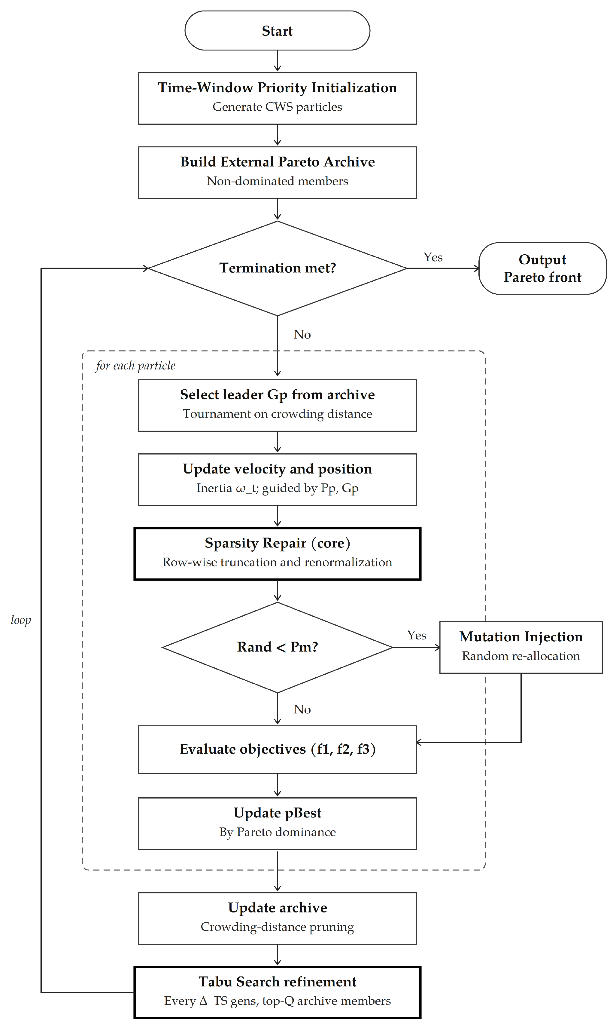
Figure 1. Flowchart of the proposed MO-HPSO-TS-SR algorithm.
Processes 14 02181 g001
Figure 2. Anytime convergence of the three algorithms on the Liyang instance under the equal 22,500-FE budget: (a) normalized hypervolume and (b) inverted generational distance versus the number of function evaluations.
Processes 14 02181 g002
Figure 3. Aggregated Pareto fronts of the three algorithms on the Liyang instance.
Processes 14 02181 g003
Figure 4. Module-level ablation across the three problem scales.
Processes 14 02181 g004
Figure 5. Region- and objective-resolved contribution of Tabu Search on the Liyang instance.
Processes 14 02181 g005
Figure 6. Performance of the three algorithms across problem scales.
Processes 14 02181 g006
Figure 7. Route-order sensitivity.
Processes 14 02181 g007
Figure 8. Fairness of the workload-balance objective.
Processes 14 02181 g008
Table 1. Notation used in the mathematical model.
SymbolDescriptionUnit
I , n a Set of work areas; number of areas
C , n c Set of cooperatives; number of cooperatives
M , n m Set of tractors; total number of tractors
M c , K c Tractors of cooperative c; cardinality
c o ( m ) Cooperative owning tractor m
W i Workload of area iha
a i ,     b i Time window of area ih
d p ,   q Haversine distance between nodes p and qkm
η Work efficiency (identical across all tractors)ha/h
ν Travel speed (identical across all tractors)km/h
c t Per-kilometer transfer costCNY/km
x i ,   m Workload of area i assigned to tractor mha
σ m Service sequence of tractor m
t i , m s , t i , m e Start/end time of tractor m at area ih
In d p , q , the nodes p and q may be either work-area indices in I or cooperative-depot indices in C .
Table 2. Hyperparameter settings for all three algorithms.
ParameterSymbolMO-HPSO-TS-SRNSGA-II-CWSHTSMOGA-CWS
Population/swarm size N s 505050
Function-evaluation budget (per run) B F E 22,50022,50022,500
Generations to budget (approx.) T g e n 310 450 310
Inertia weight range ω m i n , ω m a x [0.4, 0.9]N/AN/A
Acceleration coefficients c 1 = c 2 1.5N/AN/A
Crossover probability p c N/A0.90.9
Mutation probability p m 0.10.10.1
Sparsity threshold ratio ρ 0.05N/AN/A
External archive size cap A m a x 100N/AN/A
TS interval (generations) T S 5N/A5
TS seeds per call Q 3N/A3
TS step limit S 8N/A8
TS neighbors per step N n b r 5N/A5
Tabu tenure L 5N/A5
Table 3. Performance comparison on the Liyang instance.
IndicatorMO-HPSO-TS-SRNSGA-II-CWSHTSMOGA-CWS
HV ↑1.2131 ± 0.01551.0640 ± 0.03821.1441 ± 0.0280
IGD ↓0.0790 ± 0.00360.1696 ± 0.02230.1370 ± 0.0189
SP ↓0.0214 ± 0.00310.0347 ± 0.00560.0353 ± 0.0055
Front size99.7 ± 1.150.0 ± 0.050.0 ± 0.0
mean ± std over 20 runs; ↑/↓ indicate the preferred direction. Bold values indicate the best results.
Table 4. Pairwise Wilcoxon signed-rank tests and Cliff’s δ effect sizes on the Liyang instance.
ComparisonHVIGDSP
MO-HPSO vs. NSGA-IIp = 2.7 × 10⁻⁴ *
(δ = +1.000, large)
p = 2.7 × 10⁻⁴ *
(δ = +1.000, large)
p = 2.7 × 10⁻⁴ *
(δ = +0.980 large)
MO-HPSO vs. HTSMOGAp = 2.7 × 10⁻⁴ *
(δ = +0.980, large)
p = 2.7 × 10⁻⁴ *
(δ = +1.000, large)
p = 2.7 × 10⁻⁴ *
(δ = +0.990, large)
HTSMOGA vs. NSGA-IIp = 2.7 × 10⁻⁴ *
(δ = +0.950, large)
p = 2.7 × 10⁻⁴ *
(δ = +0.745, large)
p = 0.77
(δ = −0.060, negligible)
Positive δ indicates the first algorithm performs better. Reported p-values are paired Wilcoxon signed-rank tests, Holm-adjusted within each indicator (family size m = 3); * denotes significance at α = 0.05 .
Table 5. Module-level 2 × 2 ablation (SR × TS) of hypervolume across the three instances.
ScaleBase (PSO)+SR+TSFull (+SR + TS)SR ContributionTS ContributionSR × TS Interaction
Small1.20561.22951.20331.2417+0.0385+0.0122+0.0145
Medium1.02861.14391.07421.1484+0.0742+0.0045 †−0.0410
Large0.97951.09311.03981.1218+0.0820+0.0287−0.0316
All values are hypervolume (higher is better). † The TS contribution at the Medium scale is not statistically significant (Full vs. +SR: Holm-adjusted p = 0.279 ); all other Full-vs-corner differences are significant at α = 0.05 .
Table 6. Cross-scale performance summary.
ScaleInstanceAlgorithmHV ↑IGD ↓SP ↓
Small10 areas
5 tractors
2 cooperatives
MO-HPSO-TS-SR1.2462 ± 0.01200.0730 ± 0.01610.0228 ± 0.0068
NSGA-II-CWS1.0441 ± 0.02010.1353 ± 0.01440.0343 ± 0.0124
HTSMOGA-CWS1.0869 ± 0.01010.1136 ± 0.01010.0320 ± 0.0056
Medium20 areas
15 tractors
5 cooperatives
MO-HPSO-TS-SR1.2131 ± 0.01550.0790 ± 0.00360.0214 ± 0.0031
NSGA-II-CWS1.0640 ± 0.03820.1696 ± 0.02230.0347 ± 0.0056
HTSMOGA-CWS1.1441 ± 0.02800.1370 ± 0.01890.0353 ± 0.0055
Large40 areas
30 tractors
8 cooperatives
MO-HPSO-TS-SR1.1915 ± 0.01650.0814 ± 0.00400.0168 ± 0.0019
NSGA-II-CWS0.6841 ± 0.03550.2981 ± 0.02550.0286 ± 0.0046
HTSMOGA-CWS1.0800 ± 0.02780.1298 ± 0.02450.0303 ± 0.0067
mean ± std over 20 runs per algorithm per scale. Bold values indicate the best results.
Table 7. Wall-clock runtime comparison.
ScaleMO-HPSO-TS-SRNSGA-II-CWSHTSMOGA-CWS
Small7.44 ± 2.1915.27 ± 4.1814.53 ± 3.95
Medium17.20 ± 3.0224.12 ± 4.2525.54 ± 4.46
Large29.68 ± 3.0532.13 ± 4.0638.06 ± 7.31
mean ± std seconds per run.
Disclaimer/Publisher’s Note: The statements, opinions and data contained in all publications are solely those of the individual author(s) and contributor(s) and not of MDPI and/or the editor(s). MDPI and/or the editor(s) disclaim responsibility for any injury to people or property resulting from any ideas, methods, instructions or products referred to in the content.