An Interpretable Deep Transfer Learning Approach for Drilling Operation State Identification

Abstract

Accurate identification of drilling operation states is essential for improving drilling efficiency and operational safety. However, existing methods often suffer from limited temporal feature extraction capability, weak cross-well generalization, and insufficient model interpretability. To address these issues, this study proposes a drilling-state recognition framework based on MultiHead-BiLSTM and low-rank adaptation (LoRA) transfer learning. The MultiHead-BiLSTM model combines multi-head attention with bidirectional long short-term memory to capture both critical temporal segments and global sequential dependencies in drilling time series data. To improve cross-well adaptability while reducing training computational cost, a parameter-efficient LoRA fine-tuning strategy is introduced within the transfer learning framework. In addition, SHAP-based feature attribution and attention visualization are employed to enhance model interpretability. Experimental results show that the proposed method achieves an accuracy of 95.11% and an F1-score of 94.00%, outperforming LSTM, GRU, BiLSTM, and Transformer baselines. The LoRA-based transfer strategy reduces the cross-well error rate to 1.91%, compared with 8.79% for direct transfer and 4.48–5.39% for partial-layer freezing methods. Interpretability analysis qualitatively suggests that bit depth, weight on bit, and block position contribute strongly to drilling-state discrimination, while attention visualization qualitatively suggests that the model tends to focus on operational transition periods. The proposed framework provides an effective and computationally efficient solution for intelligent drilling-state recognition and cross-well deployment.

1. Introduction

Accurate identification of drilling operation states is vital for operational safety, efficiency, and cost control [1,2]. These states represent distinct operational modes of the drilling process, including drilling, tripping in, tripping out, and static conditions. As drilling proceeds, frequent state switching according to operational demands causes fluctuations in parameters including hole depth, hook load, and torque. Continuous sensor monitoring records these parameters as logging data, which reveal both the real-time equipment condition and the interaction between drilling dynamics and formation responses. Drilling-state recognition relies on analyzing the temporal variation of these measurements [3,4]. Because each state exhibits distinct parameter patterns, the task is intrinsically complex and dynamic. It represents a typical time series classification problem involving high-dimensional, noisy, and inter-correlated data streams collected from multiple sensors. Extracting discriminative features and ensuring accurate classification remain central challenges. Recognition accuracy directly affects drilling efficiency and cost: timely identification allows operators to adjust parameters and optimize strategies, improving penetration rate, reducing unplanned downtime, and lowering overall expenses. Hence, reliable state recognition underpins safe and efficient drilling and supports intelligent drilling automation and decision-making systems [5,6,7].

Advances in logging technology have established dynamic monitoring of time series data as a standard method for recognizing drilling operation states [8]. These datasets typically include more than thirty real-time parameters that capture critical diagnostic information. Nevertheless, several challenges remain. The diversity and irregularity of operational patterns often result in complex nonlinear parameter behavior. Imbalanced data distribution is another concern, as rotary drilling samples greatly exceed those representing idle rotation at the bottom or static conditions. In addition, a single operational action can simultaneously affect multiple parameters, leading to strong feature coupling. The presence of noise, missing values, and outliers further reduces model reliability. Achieving consistent and robust recognition performance under such circumstances remains a considerable challenge.

Early work mainly used threshold rules and expert heuristics. While simple and practical, these methods depend heavily on human experience and single-parameter analysis, resulting in rigid behavior and poor adaptability to changing downhole conditions [9]. With the rise of data-driven paradigms, machine learning has shown stronger capability in feature extraction, pattern discovery, and correlation modeling for complex drilling data [10]. By automatically identifying informative features from large-scale sequences, learning-based methods have markedly improved recognition performance, shifting research from rule-based to intelligent, data-driven approaches [11,12,13].

Recent research has primarily concentrated on improving data processing, feature extraction, and model optimization. One of the major challenges lies in class imbalance [14]: rotary drilling states account for the majority of samples, whereas idle and static conditions are relatively rare. Models trained on such skewed datasets often exhibit a strong bias toward majority classes, leading to poor recognition of minority states and limited generalization capability [15]. Existing solutions can be broadly divided into data-level and algorithm-level strategies [16]. Data-level approaches, including under-sampling, over-sampling, and generative data synthesis, seek to rebalance datasets, while algorithm-level methods introduce weighted learning, cost-sensitive optimization, or ensemble frameworks. Among these, data-level techniques remain prevalent due to their ease of implementation and adaptability across models.

Effective feature representation plays an equally crucial role in drilling operation recognition [17]. Conventional feature selection approaches, including expert-driven selection [18], principal component analysis [19], embedded methods [20], wrapper techniques [21], and filter-based strategies [22], aim to preserve the most informative variables [23]. Nevertheless, these methods often fail to account for the temporal and spectral characteristics intrinsic to drilling data. The parameters exhibit strong nonlinearity and context dependence, with varying significance across different operational states and frequent interference from noise and redundancy. As a result, conventional selection techniques struggle to capture the underlying temporal dynamics and inter-parameter correlations embedded in the data.

Drilling-state identification essentially represents a high-dimensional classification task in which model architecture plays a decisive role in performance. Traditional algorithms such as support vector machines [24], decision trees [25], and neural networks [26] each offer distinct advantages; however, their static nature limits their ability to capture the sequential dependencies characteristic of drilling data [27]. As a result, recent research has increasingly focused on deep learning frameworks that can model both temporal and multi-scale features [28,29]. Recurrent neural networks (RNNs) and one-dimensional convolutional networks (1D-CNNs) have demonstrated promising performance in modeling short- and medium-term dependencies [30]. Nonetheless, when applied to longer sequences, these architectures often encounter gradient vanishing or explosion problems, which hinder their capacity to learn extended temporal relationships. The LSTM network mitigates these issues through the use of memory cells and gating mechanisms, enabling it to effectively capture long-term dependencies and exhibit robust adaptability to complex drilling dynamics [31].

Despite such advances, three critical challenges persist.

(1)

Temporal dependency modeling remains insufficient. Shallow statistical or unidirectional recurrent models struggle with long-range dependencies, failing to capture the dynamic evolution of downhole processes.

(2)

Cross-well generalization is limited. Differences in geological formations, equipment, and operating procedures produce substantial data distribution shifts. Models trained on one well degrade when applied to another because parameters become overfitted to the source data.

(3)

Model interpretability is weak. Most deep models act as black boxes: although they yield accurate predictions, their internal reasoning is opaque, hindering trust and adoption in field operations [32].

With the advancement of intelligent drilling and digital oilfield technologies, there is an increasing demand for drilling-state recognition methods that are accurate, robust, computationally efficient, and interpretable. Rather than proposing a fundamentally new neural network architecture or transfer learning algorithm, this study aims to develop an integrated framework for cross-well drilling-state recognition under limited labeled-data conditions. To this end, a deep transfer learning framework is proposed that combines a MultiHead-BiLSTM model for temporal feature extraction, a LoRA-based adaptation strategy for parameter-efficient cross-well transfer, and a multi-level interpretability scheme incorporating SHAP analysis, attention visualization, and LoRA parameter examination. The proposed framework enables accurate drilling-state recognition while improving adaptation efficiency and model transparency. To the best of the authors’ knowledge, the combined application of LoRA-based transfer learning, SHAP interpretation, and attention visualization within a unified framework for cross-well drilling-state recognition has not been systematically investigated in previous studies.

2. Fundamental Models and Methodology

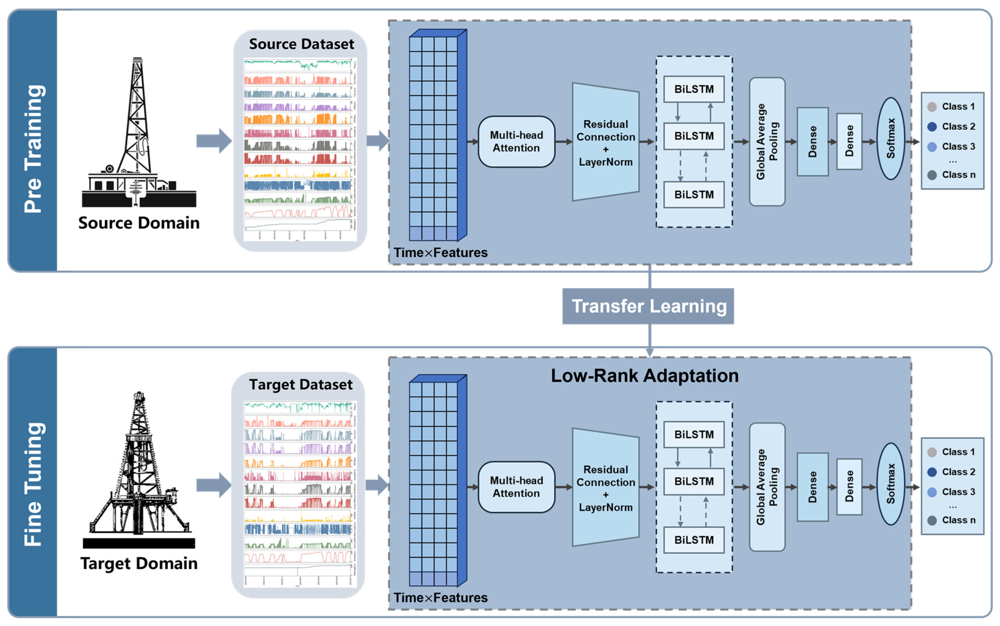
The overall framework of the proposed deep transfer learning-based drilling operation recognition method is illustrated in Figure 1. The framework comprises two primary stages: pre-training and transfer. During the pre-training stage, drilling data from the source domain undergo cleaning, normalization, and other preprocessing operations to ensure data integrity and consistency. A BiLSTM-based classification model enhanced with a multi-head attention mechanism is then trained on the processed data to obtain a pre-trained model. In the transfer stage, drilling data from the target well are preprocessed in the same manner and input into the pre-trained model. The model parameters are subsequently updated using the LoRA technique, which enables efficient fine-tuning to align with the target data characteristics. The adapted transfer model finally outputs the drilling operation classification results, achieving accurate recognition for the target well.

2.1. Classification Model Architecture

A classification model combining a multi-head attention mechanism and a BiLSTM network is developed in this study. The attention module first extracts key features from the input sequence, emphasizing information that contributes most significantly to classification. These weighted features are then passed into the BiLSTM structure, which leverages its bidirectional sequence modeling capability to capture long-term temporal dependencies. This hybrid architecture enhances both feature representation and classification accuracy.

2.1.1. Multi-Head Attention Mechanism

The multi-head attention mechanism is inspired by the human selective attention process, which focuses cognitive resources on the most task-relevant information while suppressing irrelevant details. By assigning varying weights to input features, attention mechanisms enable models to concentrate on features that have the greatest influence on prediction outcomes, thereby improving feature extraction and predictive accuracy [33]. Building on this concept, multi-head attention introduces multiple parallel attention “heads” each learning distinct feature correlations within different subspaces. 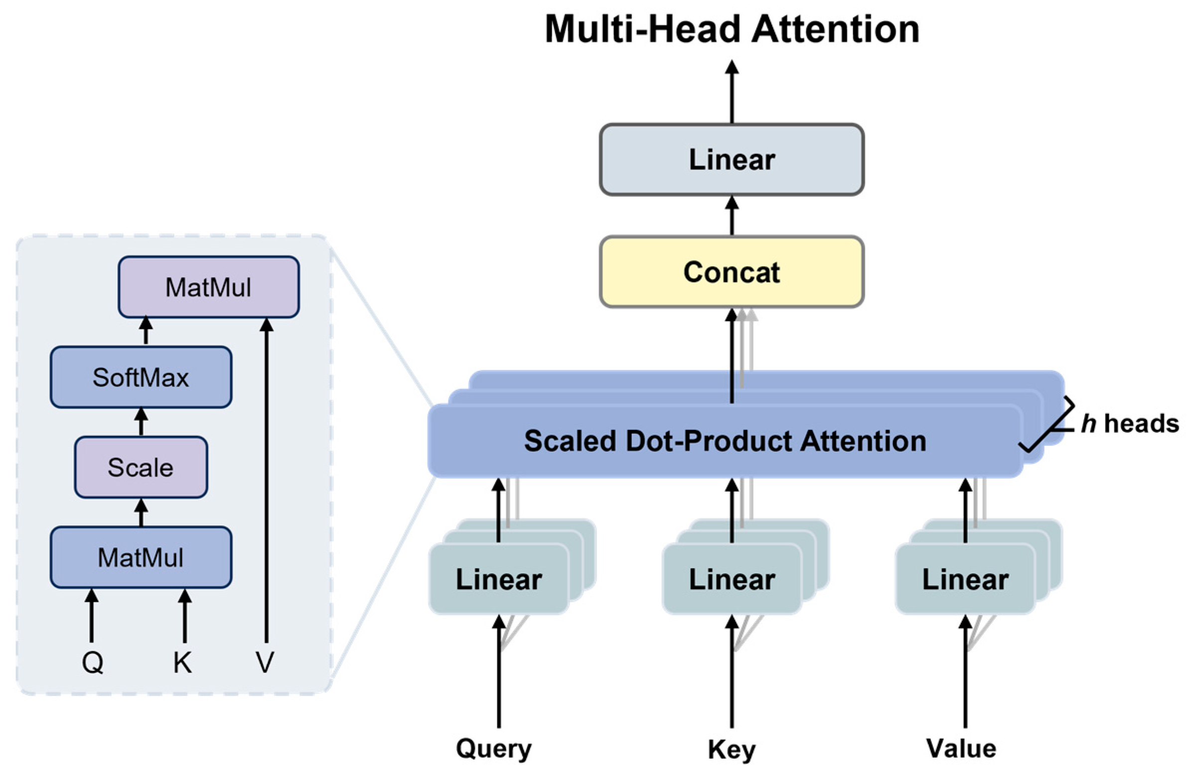This parallel design allows the model to capture dependencies across different sequence positions more comprehensively [34]. As illustrated in Figure 2, for input query, key, and value matrices Q, K, and V, the MHA mechanism generates h sets of transformed matrices $Q_i$, $K_i$, $V_i$ through linear projections:

$$Q_i=Q{W}_Q^i,K_i=K{W}_K^i,V_i=V{W}_V^i$$

(1)

where $W_Q^i$, $W_K^i$ and $W_V^i$ denote the projection matrices for the $i^{th}$ attention head.

Each head computes its output via the scaled dot-product attention:

$${\mathrm{head}}_i=\mathrm{Attention}\left(Q_i,K_i,V_i\right)=\mathrm{softmax}\left({\displaystyle \frac{Q_i{K_i}^T}{\sqrt{d_k}}}\right)V_i$$

(2)

where $d_k$ is the key dimension used to stabilize gradients by scaling the dot product.

The outputs from all heads are concatenated and linearly projected to form the final attention output:

$$\mathrm{MultiHead} \left(Q,K,V\right)=\mathrm{Concat} ({\mathrm{head}}_1,{\mathrm{head}}_2,\dots ,{\mathrm{head}}_h)W^O$$

(3)

where $W^O$ represents the output projection matrix. This mechanism allows the model to learn diverse contextual dependencies while maintaining computational efficiency.

2.1.2. Bidirectional Long Short-Term Memory Network

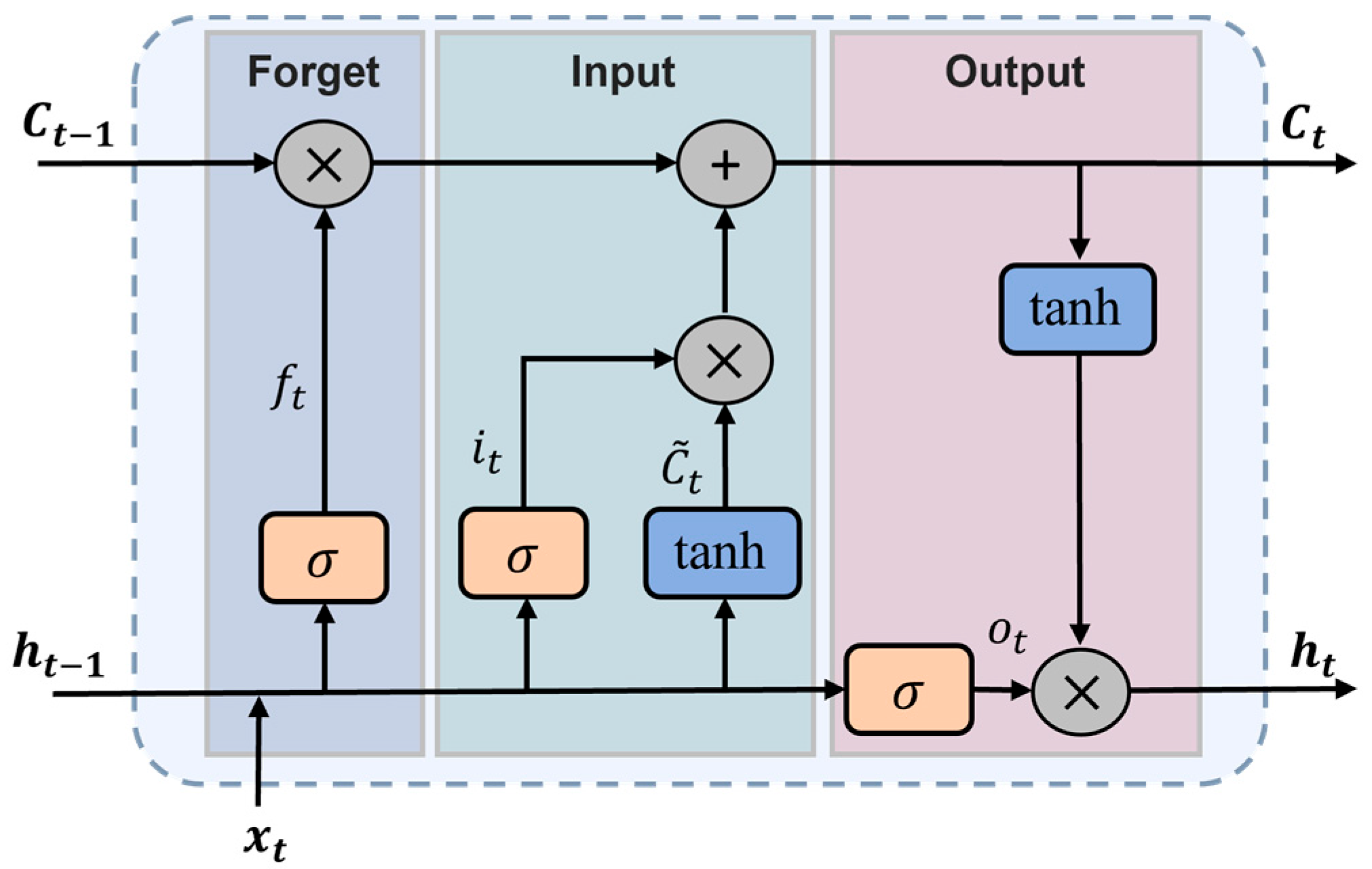
The LSTM network is a variant of the RNN that introduces gating mechanisms to mitigate vanishing and exploding gradients, thus enabling more effective modeling of long-range temporal dependencies [35]. As illustrated in Figure 3, its core structure comprises three gates: the forget gate $f_t$, the input gate $i_t$, and the output gate $o_t$. The forget gate determines which information is discarded from the cell state, the input gate regulates how new information is incorporated, and the output gate controls the information propagated to the next hidden state [36].

The computation process is defined as:

$$f_t=\sigma ({\Phi }_f{h}_{t-1}+{\Psi }_f{x}_t+b_f)$$

(4)

$$i_t=\sigma ({\Phi }_i{h}_{t-1}+{\Psi }_i{x}_t+b_i)$$

(5)

$$o_t=\sigma ({\Phi }_o{h}_{t-1}+{\Psi }_o{x}_t+b_o)$$

(6)

$${\tilde{C}}_t=\mathit{tanh}({\Phi }_c{h}_{t-1}+{\Psi }_c{x}_t+b_c)$$

(7)

$$C_t=f_t\times C_{t-1}+i_t\times {\tilde{C}}_t$$

(8)

$$h_t=o_t\times \mathit{tanh}\left(C_t\right)$$

(9)

where $\sigma \left(·\right)$ denotes the sigmoid activation function, $\Phi$ and $\Psi$ are the weight matrices for the hidden state and input, respectively, $b$ represents the bias term, and $C_t$ is the cell state at time $t$.

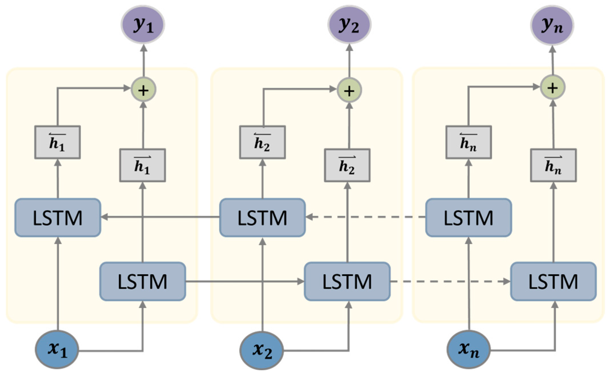
The BiLSTM extends this architecture by processing the input sequence in both forward and backward directions (Figure 4). For an input sequence $x=\left(x_1,x_2,\dots ,x_n\right)$, the forward LSTM computes hidden states $\stackrel{⃑}{h_t}$ from $x_1$ to $x_n$, while the backward LSTM computes $\stackrel{⃐}{h_t}$ in reverse. The output at each time step is the concatenation of the two:

$$y_t=[\stackrel{⃑}{h_t},\stackrel{⃐}{h_t}]$$

(10)

This structure effectively integrates contextual information from both past and future, providing a more comprehensive representation of temporal dependencies.

2.2. Deep Transfer Learning

Deep transfer learning integrates the representational power of deep learning with the knowledge-sharing capability of transfer learning, substantially improving model generalization [37]. Conventional deep learning models rely on the independent and identically distributed (i.i.d.) assumption, which often does not hold for drilling data due to differences in geological formations, drilling parameters, and downhole conditions. By explicitly modeling latent correlations between source and target domains, deep transfer learning relaxes the i.i.d. constraint and achieves better adaptability under complex operational conditions [38].

Another major challenge in drilling-state recognition is the scarcity of high-quality labeled data. Manual labeling is time-consuming and costly, making it difficult to build large-scale training datasets. Transfer learning alleviates this limitation by leveraging pre-trained knowledge from related domains and fine-tuning the model on limited target data. This approach not only improves training efficiency but also enhances the feasibility of real-time field deployment.

To achieve efficient adaptation, this study employs the Parameter-Efficient Fine-Tuning (PEFT) strategy, which enables task-specific adaptation with minimal computational and storage overhead [39]. Within this framework, LoRA introduces low-rank trainable components into selected weight matrices, substantially reducing the number of trainable parameters while maintaining modeling capacity for target domain features [40].

Formally, given a pre-trained weight matrix:

$$W_0\in R^{d\times k}$$

(11)

where d and k denote the output and input dimensions, respectively, LoRA represents the parameter update as:

$$∆W=BA$$

(12)

with

$$A\in R^{r\times k},B\in R^{d\times r}$$

(13)

Here, $A$ projects the input to a lower-dimensional subspace, while B maps it back to the original space. The rank $r\ll \mathrm{m}\mathrm{i}\mathrm{n}(d,k)$ serves as a hyperparameter controlling the degree of parameter compression. The final updated weights are expressed as:

$$W=W_0+\alpha ·∆W$$

(14)

where $\alpha$ is a scaling factor balancing the contribution of the low-rank update.

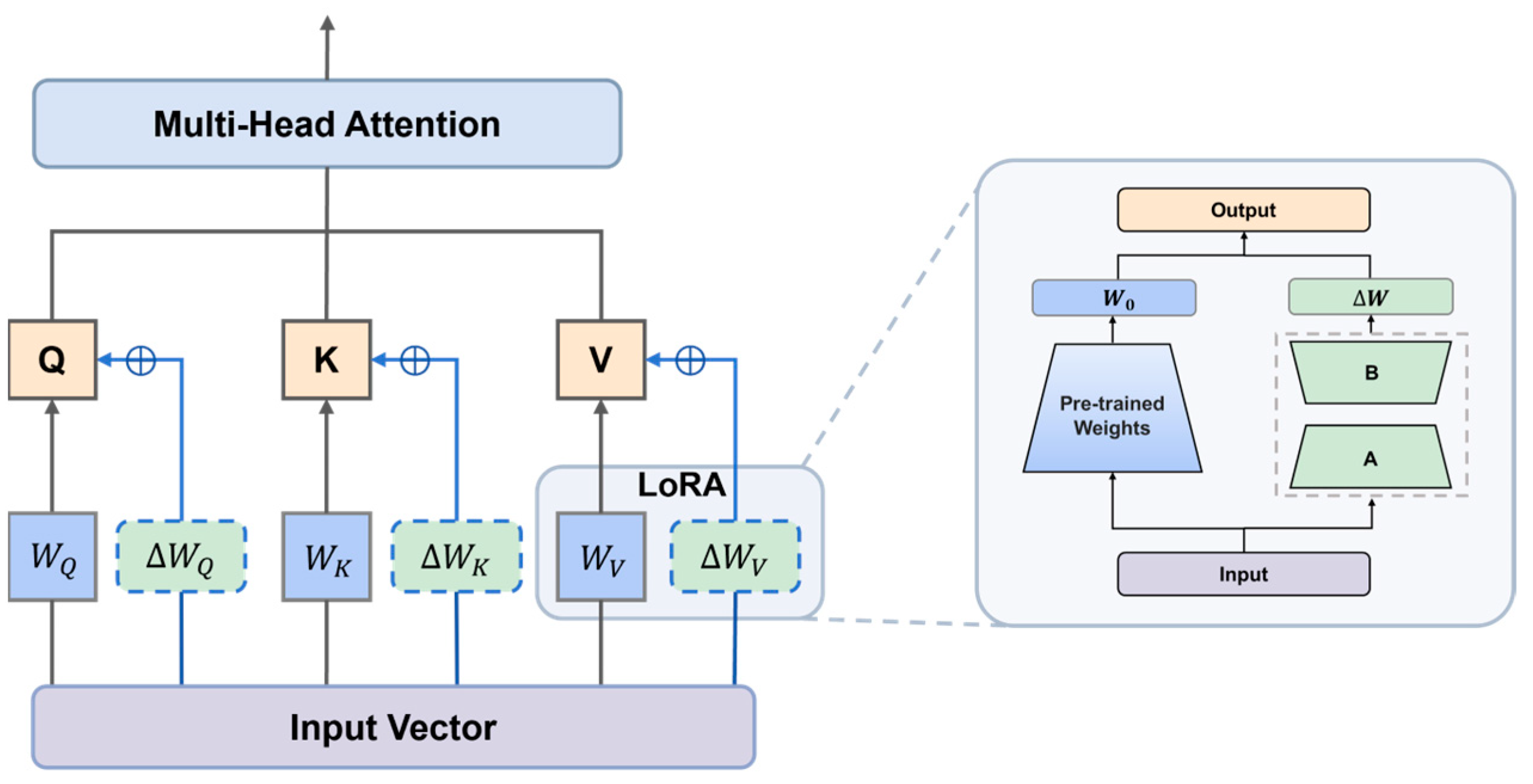
As shown in Figure 5, integrating LoRA into the multi-head attention mechanism modifies the forward computation as follows:

$$Q_i=Q\left(W_Q^i+{\alpha }_Q^i{B}_Q^i{A}_Q^i\right)=Q{W}_Q^i+{\alpha }_Q^{i}Q{B}_Q^i{A}_Q^i$$

(15)

$$K_i=K\left(W_K^i+{\alpha }_K^i{B}_K^i{A}_K^i\right)=K{W}_K^i+{\alpha }_K^{i}K{B}_K^i{A}_K^i$$

(16)

$$V_i=V\left(W_V^i+{\alpha }_V^i{B}_V^i{A}_V^i\right)=V{W}_V^i+{\alpha }_V^{i}V{B}_V^i{A}_V^i$$

(17)

During fine-tuning, the original weight matrices $W_Q^i$, $W_K^i$, $W_V^i$ remain frozen, and only $A_{*}^i$ and $B_{*}^i$ are updated. Consequently, the parameter count is reduced from $d\times k$ to $r\times \left(d+k\right)$, significantly lowering computational cost while preserving adaptability to target features.

Mechanistically, LoRA achieves a balance between knowledge preservation and domain-specific adaptation. By freezing the main network weights, the model retains the general drilling patterns learned from the source domain, while the low-rank matrices $A$ and B introduce targeted adjustments for the new domain. Matrix $A$ constrains the update direction in a compact subspace to ensure stability and convergence, whereas B captures distributional shifts through up-projection. This hierarchical update mechanism allows LoRA to efficiently bridge domain gaps, achieving a favorable trade-off between transfer efficiency, stability, and generalization.

3. Dataset Processing and Construction

3.1. Data Preprocessing

The dataset employed in this study was obtained from two wells, referred to as Well A and Well B, situated in different blocks of the same oilfield and within the same drilling interval. Measurements were recorded at 5 s intervals, resulting in 851,674 valid samples from Well A and 398,314 from Well B. Data from Well A were used as the source domain to build the pre-trained model, whereas Well B served as the target domain for evaluating the performance and adaptability of the proposed transfer learning method.

Thirteen parameters were selected as feature variables, including Hole Depth, Bit Depth, Hook Load, Block Position, weight on bit (WOB), surface revolutions per minute of the rotary table (RPM), Bit RPM, Torque, standpipe pressure (SPP), strokes per minute of the mud pump (SPM), Flow In, Flow Out, and total pit volume (TPV) [41]. The temporal variations of these parameters for both the source and target domains are shown in Figure 6 and Figure 7. As illustrated, the raw data contain noise, outliers, and missing values. To ensure data quality, both datasets underwent preprocessing, including noise reduction, outlier removal, and missing-value reconstruction.

Outliers refer to samples that deviate significantly from the overall data trend, often caused by sensor malfunction. In this study, a standard-deviation-based outlier detection method was adopted. For a given data point $x_i$, if its deviation from the mean $\mu$ exceeds three times the standard deviation $\sigma$, then it is identified as an outlier:

$$|x_i-\mu |>3\sigma$$

(18)

Detected outliers were corrected using linear interpolation, which estimates the abnormal value based on the linear relationship between its adjacent valid points:

$$x_t=x_{t-1}+{\displaystyle \frac{{x_{t+1}-x}_{t-1}}{2}}$$

(19)

where $x_t$ is the abnormal value, $x_{t-1}$ and $x_{t+1}$ are its neighboring valid samples.

Signal interruptions or storage errors during data acquisition may lead to missing values. These were repaired using spline interpolation, which fits a high-order polynomial to the data and evaluates missing points via spline basis functions:

$$x_l={\displaystyle \sum _{i=0}^N}{c}_i{B}_i\left(l\right)$$

(20)

where $x_l$ denotes the reconstructed value, $B_i\left(l\right)$ is the spline basis function, and $c_i$ represents spline coefficients estimated using the least-squares method.

Descriptive statistics for all parameters in the source and target domains are summarized in

Table 1. Statistical analysis of source domain well data.

Parameters	Mean	Median	Standard Deviation	Min	Max	Interquartile Range	Unit
Hole Depth	3610.559	2978.310	729.362	2974.000	4631.290	1469.780	m
Bit Depth	2188.229	2753.198	1554.923	0	4631.286	2903.671	m
Hook Load	958.533	748.648	642.207	54.880	3068.933	1253.075	kN
Block Position	23.368	24.964	10.718	4.800	40.696	21.939	m
WOB	5.146	0	21.019	0	119.090	0	kN
Surface RPM	14.535	0	25.162	0	79.842	21.143	rpm
Bit RPM	14.535	0	25.162	0	79.842	21.143	rpm
Torque	3.270	0	6.254	0	65.007	5.168	kN·m
SPP	8.448	0	13.356	0	39.814	17.079	Mpa
SPM	41.659	0	59.788	0	181.000	116.000	spm
Flow In	15.025	0	21.746	0	113.357	41.717	L/s
Flow Out	15.432	0.134	23.660	0	95.700	42.913	L/s
TPV	70.930	78.846	18.681	0.782	96.824	21.185	m3

and

Table 2. Statistical analysis of target domain well data.

Parameters	Mean	Median	Standard Deviation	Min	Max	Interquartile Range	Unit
Hole Depth	1781.922	1628.000	204.138	1551.767	2259.501	432.355	m
Bit Depth	1029.290	1319.506	814.122	0	2259.501	1638.852	m
Hook Load	709.262	529.138	484.940	76.035	2899.921	937.280	kN
Block Position	19.831	19.304	10.244	2.485	36.371	20.040	m
WOB	20.433	0	40.702	0	150.000	40.027	kN
Surface RPM	24.705	0	34.260	0	96.154	55.119	rpm
Bit RPM	24.705	0	34.260	0	96.154	55.119	rpm
Torque	4.734	0.019	7.826	0	70.752	6.449	kN·m
SPP	7.248	0	9.620	0	32.881	18.427	Mpa
SPM	60.462	0	76.259	0	194.000	157.000	spm
Flow In	26.914	0	33.931	0	86.939	67.925	L/s
Flow Out	17.920	0	22.149	0	100.000	46.480	L/s
TPV	67.043	69.942	9.485	23.251	84.102	11.113	m3

. In terms of mechanical loading, the mean Hook Load of the source well (958.533 kN) is notably higher than that of the target well (709.262 kN). Conversely, the mean WOB in the source well is only 5.146 kN with a median of zero, indicating that most operating conditions occur without applied bit weight, while the target well exhibits a higher mean WOB of 20.433 kN and a maximum of 150.000 kN, reflecting stronger variability. For rotational parameters, the average Surface RPM and Bit RPM in the source domain are both 14.535 rpm, substantially lower than the 24.705 rpm observed in the target domain, which also shows a broader distribution range. Similarly, Torque and circulation parameters differ noticeably: the mean torque rises from 3.270 kN·m in the source domain to 4.734 kN·m in the target domain. The mean SPP is slightly higher in the source domain (8.448 MPa) compared with the target domain (7.248 MPa), though the latter exhibits greater fluctuations. Additionally, the pump strokes and flow rates in the target domain are significantly higher. Overall, these results reveal distinct statistical shifts across wells in terms of mechanical load, rotational dynamics, and circulation parameters, underscoring the domain distribution discrepancy between wells. Such disparities highlight the necessity of incorporating transfer learning to enhance the adaptability and robustness of drilling operation recognition models across wells.

3.2. Dataset Construction

Based on expert knowledge and field experience, the source domain data were labeled using a parameter-based hierarchical calibration approach. The labeling process consisted of two stages (

Table 3. Relationship between drilling parameters and rig operational states.

Rig Operational State (Abbreviation)	Conditional Logic Description
Bit on bottom (BOB)	Bit Depth = Hole Depth
Increasing hole depth (IHD)	Bit Depth = Hole Depth || ${∆}_{\mathrm{B}\mathrm{i}\mathrm{t}\mathrm{D}\mathrm{e}\mathrm{p}\mathrm{t}\mathrm{h}}>0$ || WOB $>0$ || Surface RPM $>0$ || ${∆}_{\mathrm{T}\mathrm{P}\mathrm{V}}<0$
Bit moving downward (BMD)	Bit Depth $<$ Hole Depth || ${∆}_{\mathrm{B}\mathrm{i}\mathrm{t}\mathrm{D}\mathrm{e}\mathrm{p}\mathrm{t}\mathrm{h}}>0$ || ${∆}_{\mathrm{B}\mathrm{l}\mathrm{o}\mathrm{c}\mathrm{k}\mathrm{P}\mathrm{o}\mathrm{s}\mathrm{i}\mathrm{t}\mathrm{i}\mathrm{o}\mathrm{n}}<0$ || WOB $=0$
Bit moving upward (BMU)	Bit Depth $<$ Hole Depth || ${∆}_{\mathrm{B}\mathrm{i}\mathrm{t}\mathrm{D}\mathrm{e}\mathrm{p}\mathrm{t}\mathrm{h}}<0$ || ${∆}_{\mathrm{B}\mathrm{l}\mathrm{o}\mathrm{c}\mathrm{k}\mathrm{P}\mathrm{o}\mathrm{s}\mathrm{i}\mathrm{t}\mathrm{i}\mathrm{o}\mathrm{n}}>0$ || WOB $=0$
Drill string disconnected (DSD)	${∆}_{\mathrm{H}\mathrm{o}\mathrm{l}\mathrm{e}\mathrm{D}\mathrm{e}\mathrm{p}\mathrm{t}\mathrm{h}}=0$ || ${∆}_{\mathrm{B}\mathrm{i}\mathrm{t}\mathrm{D}\mathrm{e}\mathrm{p}\mathrm{t}\mathrm{h}}=0$ || Hook Load $\approx$ Travel Block Weight || WOB $=0$ || SPP $=0$ || Bit Depth $=0$ || Flow In/Flow Out $=0$ || SPM $=0$ || ${∆}_{\mathrm{T}\mathrm{P}\mathrm{V}}=0$
Drill string rotating (DSR)	Surface RPM $>0$ || Torque $>0$
Surface RPM equals Bit RPM (SRB)	Surface RPM = Bit Depth
Normal circulation (NC)	SPP $>0$ || Flow In $>0$ || Flow Out $>0$|| SPM $>0$
Traveling block moving upward (TBU)	${∆}_{\mathrm{B}\mathrm{l}\mathrm{o}\mathrm{c}\mathrm{k}\mathrm{P}\mathrm{o}\mathrm{s}\mathrm{i}\mathrm{t}\mathrm{i}\mathrm{o}\mathrm{n}}>0$
Traveling block moving downward (TBD)	${∆}_{\mathrm{B}\mathrm{l}\mathrm{o}\mathrm{c}\mathrm{k}\mathrm{P}\mathrm{o}\mathrm{s}\mathrm{i}\mathrm{t}\mathrm{i}\mathrm{o}\mathrm{n}}<0$

Note: “||” denotes the logical operator AND; “=’’ indicates equality; “<” and “>” represent less-than and greater-than relations, respectively; “Δ” signifies the difference between the current value and that of the previous time step.

and

Table 4. Mapping between rig operational states and drilling operation conditions.

Drilling Operation/Class Label	BOB	IHD	BMD	BMU	DSD	DSR	SRB	NC	TBU	TBD
Rotary drilling/0	1	1	0	0	0	1	1	1	0	1
Sliding drilling/1	1	1	0	0	0	0	1	1	0	1
Making connection/2	1	0	0	0	1	0	1	0	1/0	1/0
Circulating (rig stopped) + rotation/3	1	0	0	0	0	1	1	1	0	0
Circulating (rig stopped)/4	1	0	0	0	0	0	1	1	0	0
Idle rotation at bottom/5	1	0	0	0	0	1	1	0	0	0
Static (during drilling)/6	1	0	0	0	0	0	1	0	0	0
Tripping in/7	0	0	1	0	0	0	1	0	0	1
Tripping out/8	0	0	0	1	0	0	1	0	1	0
Washing down/9	0	0	1	0	0	0	1	1	0	1
Reaming down/10	0	0	1	0	0	1	1	1	0	1
Back reaming/11	0	0	0	1	0	1	1	1	1	0
Off-bottom circulation + rotation/12	0	0	0	0	0	1	1	1	0	0
Off-bottom circulation/13	0	0	0	0	0	0	1	1	0	0
Off-bottom rotation/14	0	0	0	0	0	1	1	0	0	0
Static (tripping)/15	0	0	0	0	0	0	1	0	0	0

Notes: 1 = condition satisfied/true; 0 = condition not satisfied/false.

).

In the first stage, the operational state of the drilling rig was determined according to the dynamic variations in key parameters, such as Hole Depth, Bit Depth, and Block Position. In the second stage, the downhole drilling conditions were inferred by combining multiple parameters and logical relationships within each rig operation state.

This two-level calibration framework integrates dynamic characteristics of logging parameters with expert constraints, ensuring both the accuracy and engineering interpretability of the operational labels. The labeled dataset provides a reliable foundation for training and evaluating the subsequent deep learning models.

To analyze class separability and the inherent clustering structure among different drilling conditions, the labeled pre-training dataset was visualized using t-distributed stochastic neighbor embedding (t-SNE). This method preserves local neighborhood relationships in the low-dimensional embedding space and provides an intuitive representation of clustering behavior among different operational states [42].

The t-SNE visualization is presented in Figure 8, where the horizontal and vertical axes represent the two embedded dimensions. The results indicate that different operational states exhibit distinct distributional patterns. Rotary drilling, sliding drilling, and circulating (rig stopped) with rotation show partial overlaps, suggesting fuzzy boundaries among these states. Sliding drilling and tripping in overlap locally, reflecting similarities in block movement and rotational features. In contrast, off-bottom circulation with rotation and idle rotation at bottom samples appear more dispersed, with less distinct clustering behavior. The visualization results illustrate the distribution characteristics and potential inter-class overlaps among different drilling states. These observations are intended to provide qualitative insights into the data distribution and should not be interpreted as evidence for model design or performance evaluation.

4. Experimental Results and Analysis

4.1. Model Pre-Training

All model training was conducted within the PyCharm 2025.1 integrated development environment using the PyTorch 2.5.1 deep learning framework. All experiments were conducted using Python 3.12 and PyTorch. Scikit-learn was employed for data preprocessing and model evaluation, while SHAP was used for interpretability analysis. The models were trained on a workstation equipped with an Intel Core i9 processor, 64 GB RAM, and an NVIDIA RTX-series GPU. To comprehensively evaluate the performance of the proposed MultiHead-BiLSTM classification model, both prediction accuracy and training efficiency were examined. Classification performance was assessed using the confusion matrix, accuracy, precision, recall, and F1 score, providing a full depiction of both accuracy and stability. Training efficiency was evaluated based on the time to convergence.

The dataset was divided into training, validation, and test sets in a ratio of 6:2:2, which yielded stable results across repeated experiments. The training set was used for model training, while the validation set was employed for hyperparameter optimization, including the grid search of the LoRA parameters. The test set was reserved exclusively for the final performance evaluation and was not involved in model training or hyperparameter selection. Prior to training, feature normalization was performed using Min–Max scaling, and the same transformation was subsequently applied to the validation and test sets to ensure consistency across datasets. During training, accuracy and loss were monitored dynamically to track model performance. To prevent overfitting and improve convergence, EarlyStopping and ReduceLROnPlateau mechanisms were incorporated. Training was halted when validation loss failed to improve for ten consecutive epochs, while the learning rate was halved upon loss stagnation. The initial learning rate was set to 0.001. Considering the inherent class imbalance in the drilling operation dataset, a class-weighted loss function was adopted during model training. The class weights were calculated using only the training set to avoid information leakage from the validation and test sets. For each drilling-state class (c), the weight was defined as:

$$w_c={\displaystyle \frac{N}{C\times n_c}}$$

(21)

where $N$ is the total number of training samples, $C$ is the number of drilling-state classes, and $n_c$ is the number of training samples belonging to class $c$. In this way, minority classes with fewer samples were assigned larger weights, whereas majority classes were assigned smaller weights. The calculated class weights were incorporated into the sparse categorical cross-entropy loss function to reduce the dominance of majority classes during optimization.

Multiple experiments with varied parameter settings were conducted to determine the optimal configuration, as summarized in

Table 5. Model parameter settings.

Module	Parameter	Setting
Multi-Head Attention	Num Heads	8
	Key Dim	64
BiLSTM	Units	128
	Dropout Rate	0.3
Fully Connected Layer	Dense (Units)	128
	Activation Function	ReLU
Output Layer	Dense (Units)	16
	Activation Function	Softmax
Model Training	Loss Function	Sparse Categorical Cross-Entropy
	Optimizer	Adam
	Initial Learning Rate	0.001
	Maximum Epochs	150
	Batch Size	128

.

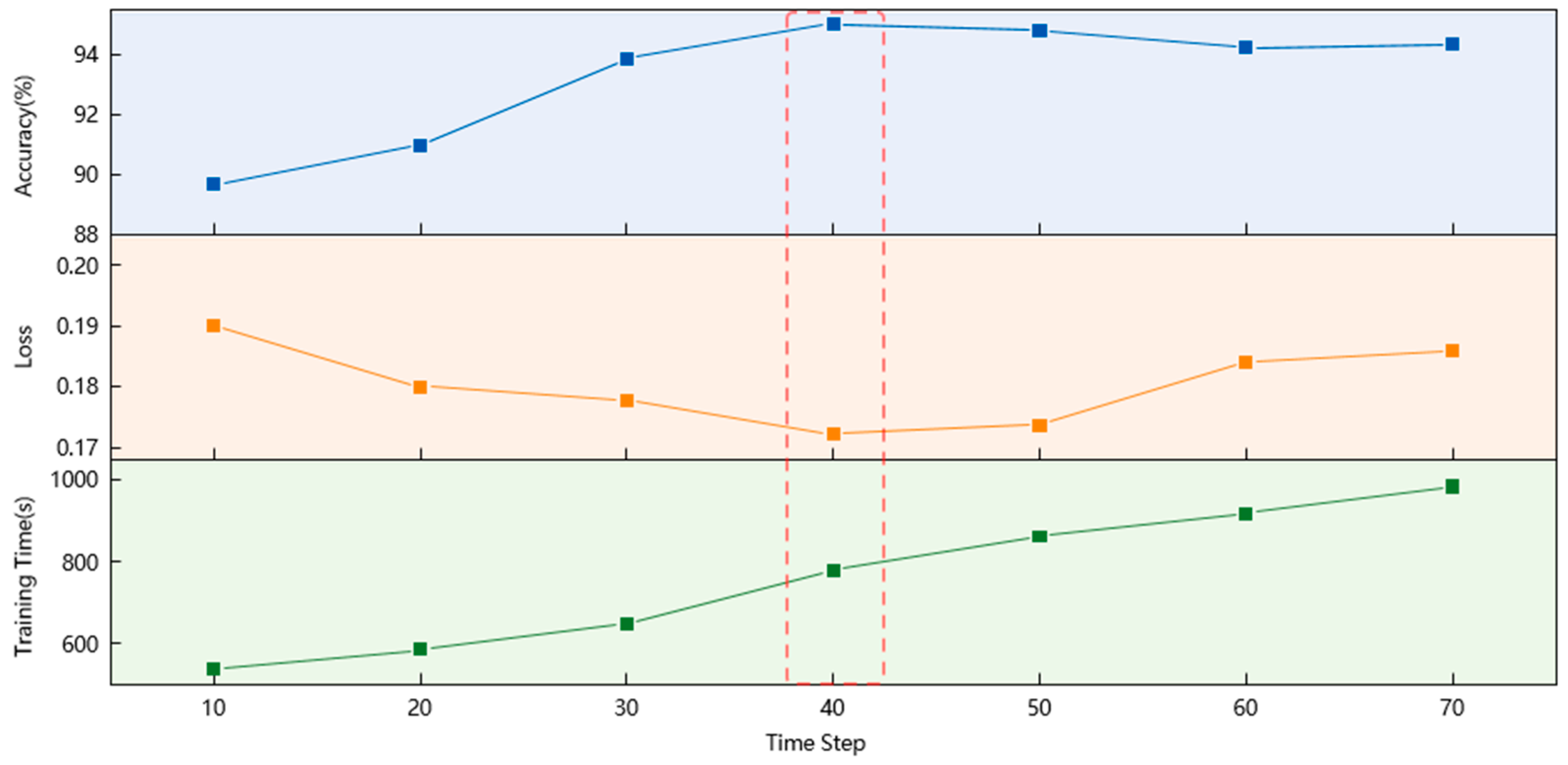
Among the hyperparameters, the time step length plays a pivotal role in sequence modeling, influencing the model’s capacity to capture temporal dependencies, its convergence speed, and its prediction accuracy. A shorter step size limits global feature extraction, whereas an excessively large step size increases computational cost and training time. To identify an optimal balance, comparative experiments were performed, considering accuracy, loss, and training duration. As shown in Figure 9, training time increases with longer time steps, while accuracy and loss do not exhibit monotonic trends. The model achieved optimal accuracy and loss performance when the time step was set to 40, which was therefore adopted for subsequent experiments.

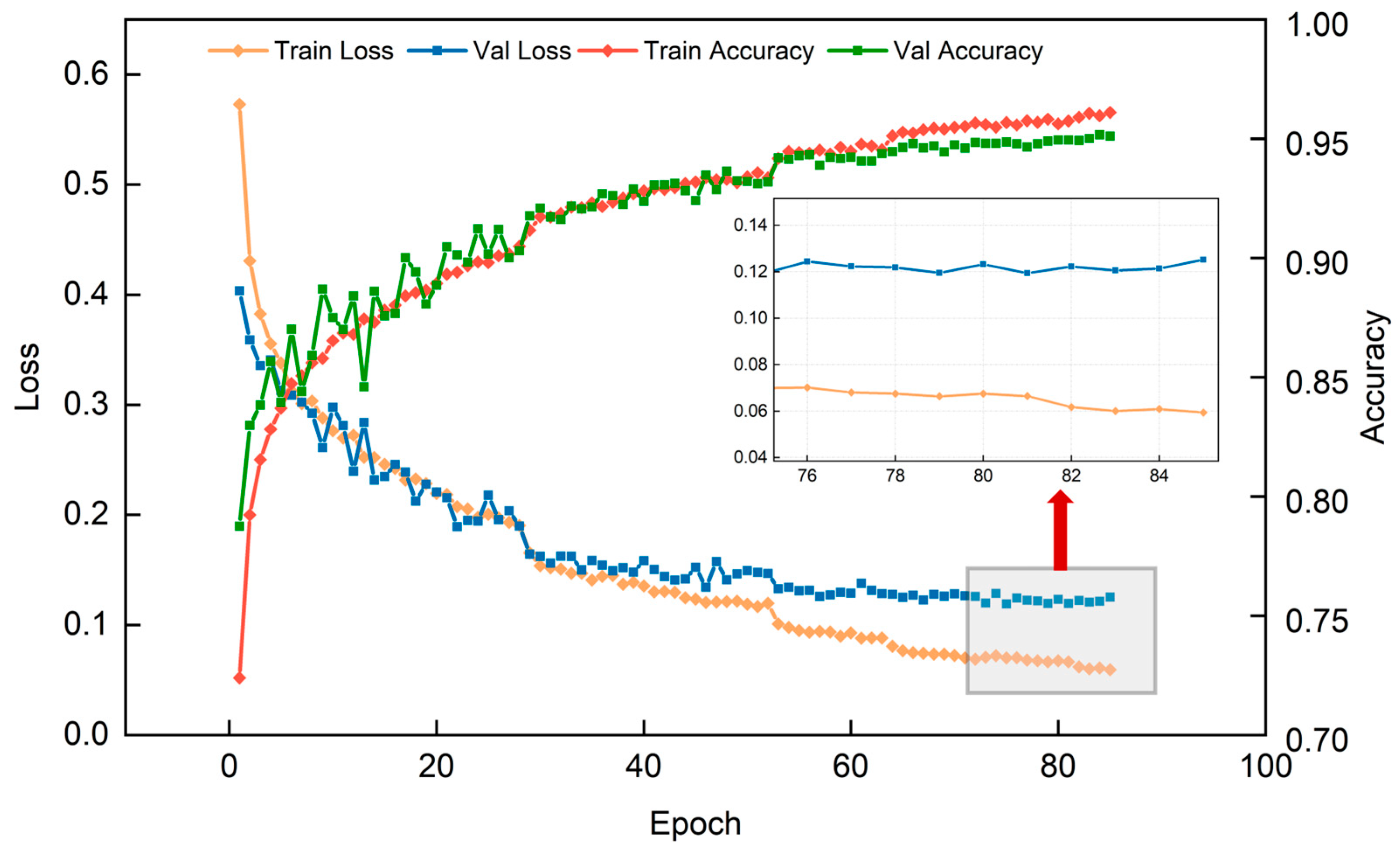
The variations in training and testing losses and accuracies over iterations are illustrated in Figure 10. At the early training stage, the loss decreased rapidly and accuracy improved steadily as the model adapted to data patterns. Around 75 epochs, validation loss stabilized, indicating convergence. To prevent overfitting, training was terminated early at epoch 85, when the validation loss reached 0.1252 and accuracy attained 0.9511, confirming stable convergence and good generalization.

4.2. Model Performance Analysis

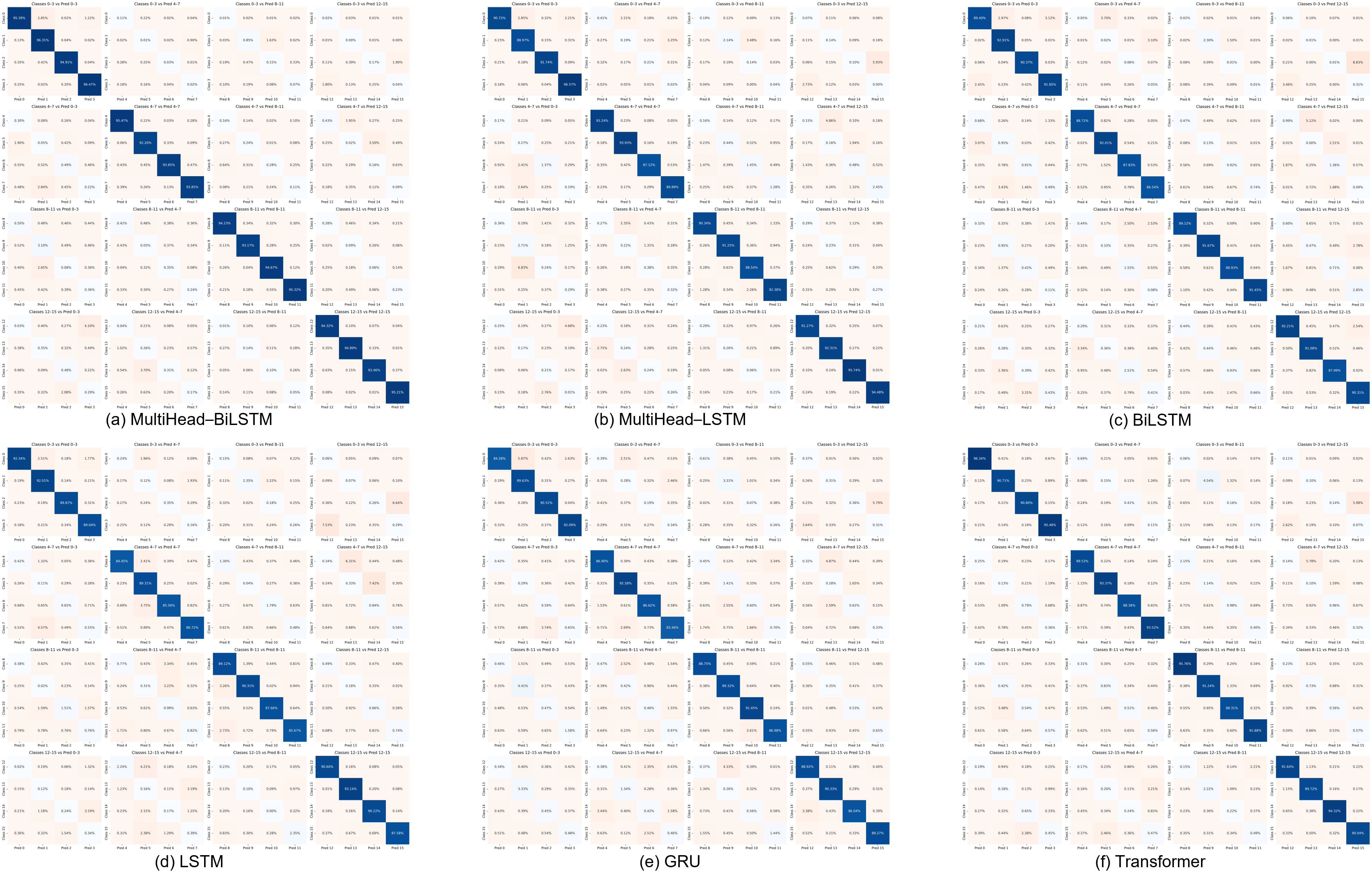
To benchmark the proposed approach, several representative sequence models were selected for comparison, including MultiHead-LSTM, BiLSTM, LSTM, GRU, and Transformer. All models shared identical data partitioning, time step, batch size, initial learning rate, optimizer, learning rate scheduler, and early stopping settings to ensure fair and unbiased comparison. The confusion matrices of all models are shown in Figure 11.

The MultiHead-BiLSTM model achieved the best overall classification performance, with fewer cross-class misclassifications and clearer decision boundaries. Compared with LSTM, BiLSTM improved discrimination capability by capturing bidirectional temporal dependencies. Furthermore, the superior performance of MultiHead-BiLSTM over BiLSTM indicates that the multi-head attention mechanism effectively enhances the model’s ability to focus on critical temporal features. These results demonstrate the complementary contributions of bidirectional sequence modeling and attention mechanisms to drilling-state recognition.

Although the overall performance was satisfactory, several operational states remained susceptible to misclassification. In particular, confusion occasionally occurred between circulating (rig stopped) and off-bottom circulation due to their similar hydraulic characteristics, such as pump pressure and flow rate. In addition, sliding drilling and tripping in showed partial overlap because of similar short-term temporal patterns within the selected observation window. These similarities reduce class separability and account for the majority of classification errors observed in the confusion matrix.

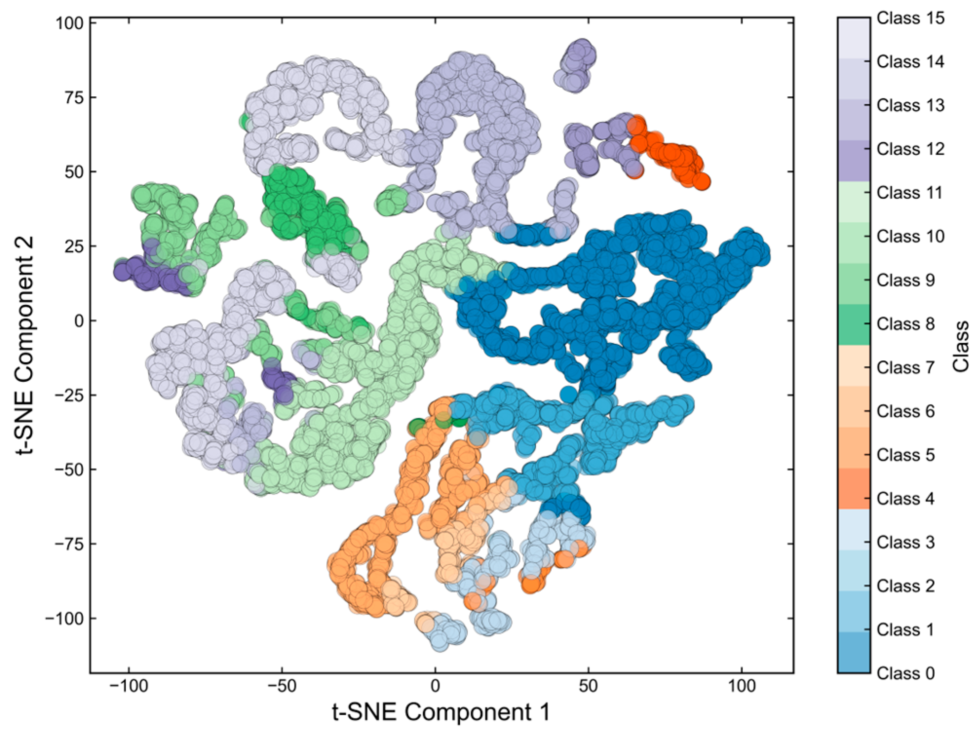
The confusion matrix patterns are generally consistent with the distribution characteristics observed in the t-SNE visualization, where several operational states exhibit partial overlaps in the feature space. This consistency suggests that the observed classification errors are closely related to the intrinsic similarity of drilling parameters among certain operational states rather than random model predictions. Overall, the results demonstrate that the MultiHead-BiLSTM model effectively combines the strengths of bidirectional temporal dependency modeling and attention-based feature focusing. By jointly capturing contextual information and critical temporal patterns, the proposed framework reduces misclassification under ambiguous operational conditions and achieves superior recognition performance compared with the selected benchmark models.

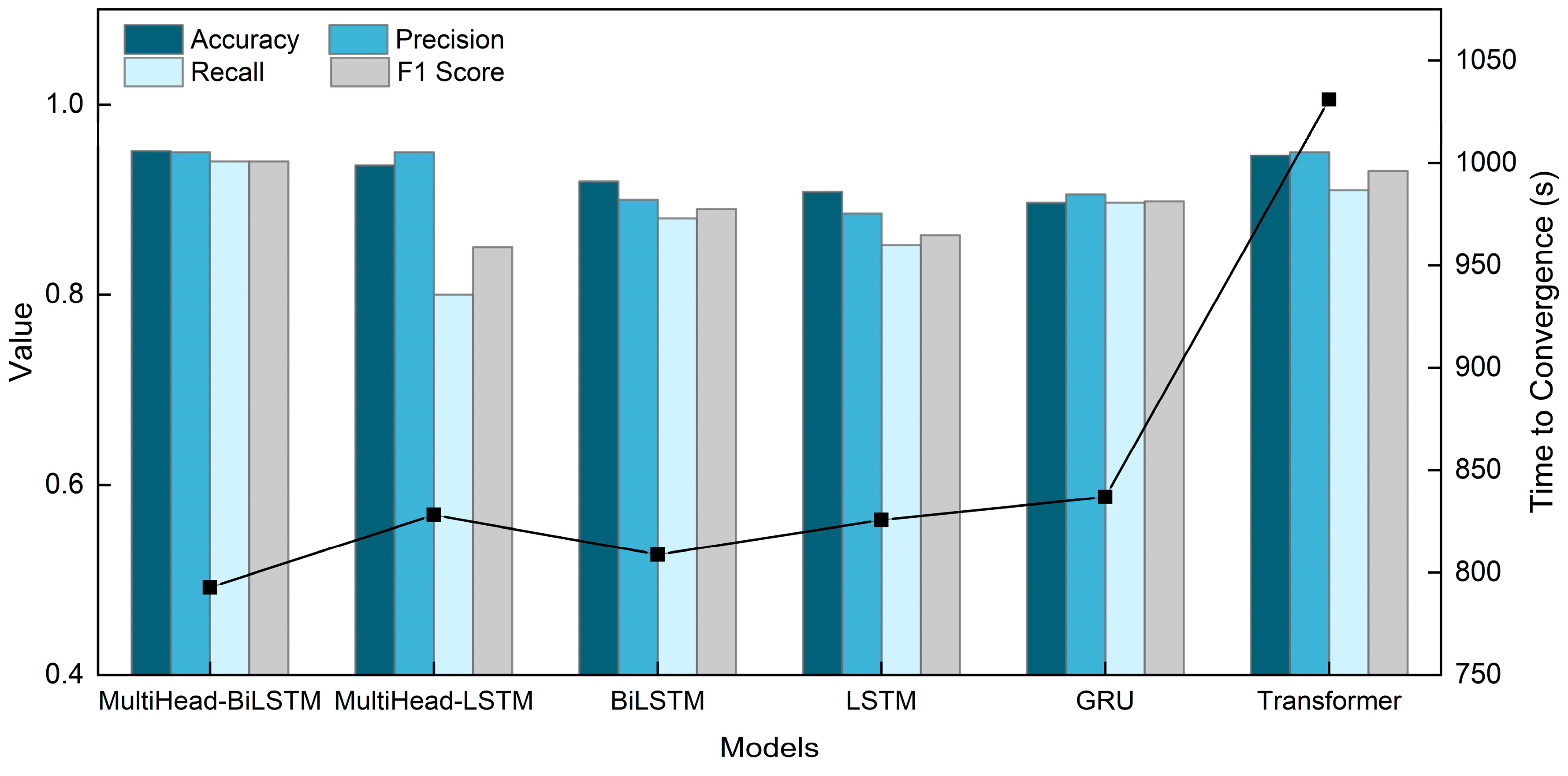
A detailed comparison of model performance and training efficiency is illustrated in Figure 12, encompassing accuracy, precision, recall, F1 score, and convergence time. The MultiHead-BiLSTM achieved an accuracy of 95.11% and an F1 score of 94.00%, with precision and recall of 95.00% and 94.00%, respectively, indicating strong classification robustness. The Transformer attained similar precision and accuracy values (95.00% and 94.64%) but exhibited a lower recall of 91.00%, leading to a reduced F1 score of 93.00%. In addition, its training time reached 1031 s, significantly exceeding the 792.70 s required by the MultiHead-BiLSTM, revealing a clear trade-off between accuracy and computational efficiency.

The MultiHead-LSTM achieved 95.00% precision but only 80.00% recall and 85.00% F1, indicating weaker stability under ambiguous conditions. Traditional unidirectional models, LSTM and GRU, delivered lower overall accuracy (90.83% and 89.68%) and F1 scores (86.27% and 89.83%), reflecting their limited ability to capture complex temporal dependencies. The BiLSTM, benefiting from bidirectional structure, improved to an F1 of 89.00%, but still fell short of attention-enhanced models.

In summary, the MultiHead-BiLSTM model achieved the best overall performance among the selected benchmark models, showing improvements in classification accuracy, generalization capability, and convergence efficiency. These results suggest that the proposed framework is a promising approach for complex drilling-state identification while maintaining a reasonable computational cost.

4.3. Transfer Learning Effectiveness Analysis

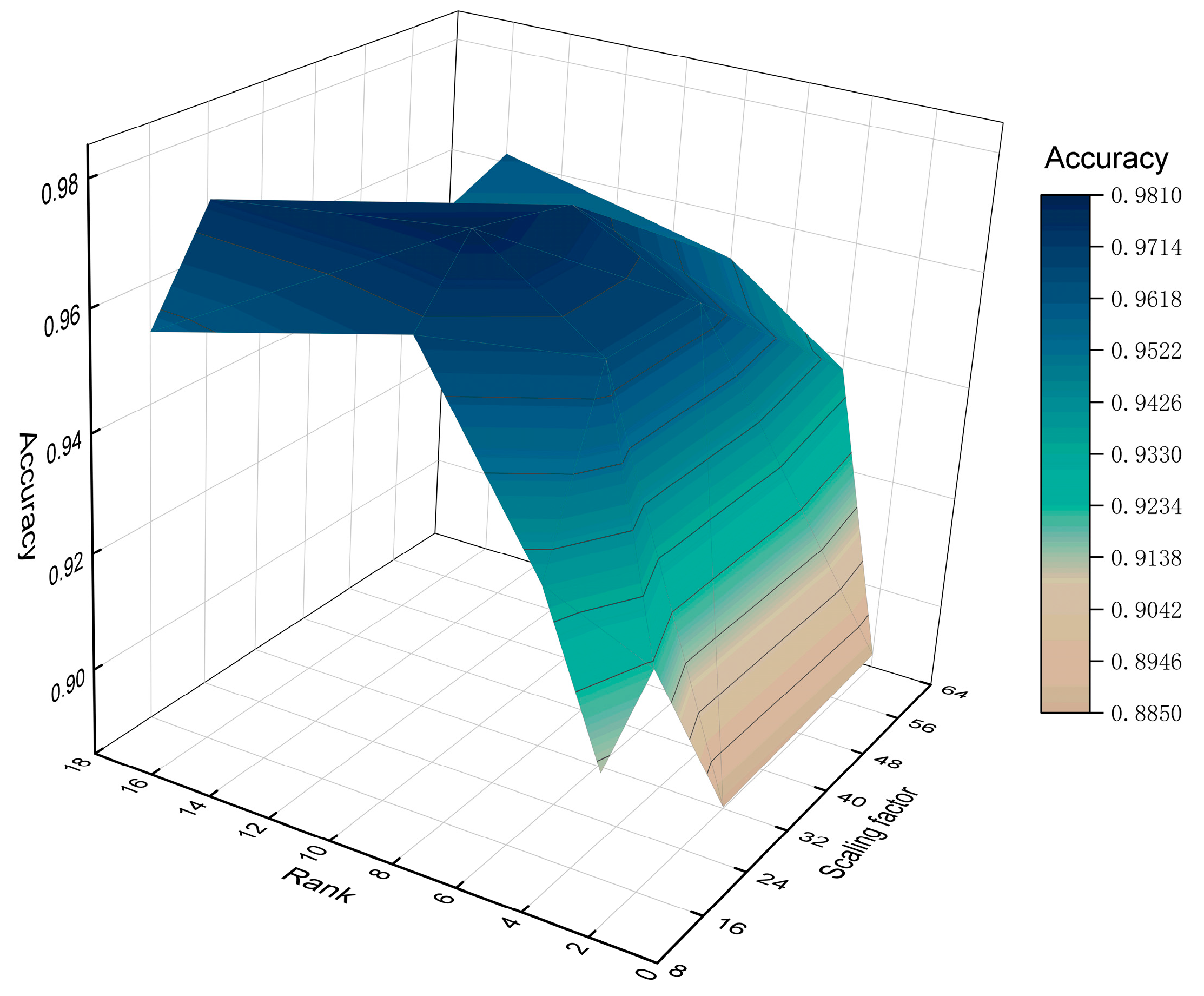
In the LoRA approach, two critical hyperparameters are the rank of low-rank decomposition ($r$) and the scaling factor ($\alpha$) that controls the contribution of the low-rank update to the overall weights. To evaluate their influence on cross-well transfer performance, a grid-search-based sensitivity analysis was conducted, and the results are presented in Figure 13. Among the tested parameter combinations, the highest classification accuracy (0.9809) was achieved when $r=8$ and $\alpha =16$. Therefore, this configuration was selected for subsequent experiments.

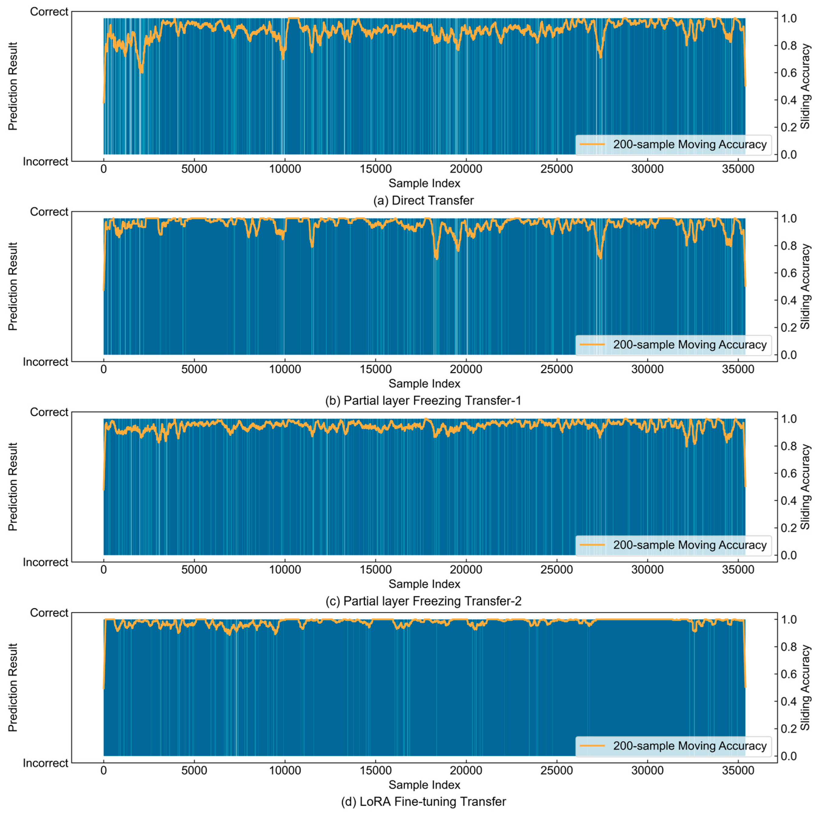
To further verify the effectiveness of LoRA fine-tuning for cross-block drilling operation recognition, several transfer strategies were compared: (1) direct transfer, applying source domain model parameters directly without modification; (2) attention layer freezing, training only the BiLSTM modules; (3) BiLSTM layer freezing, training only the attention modules; (4) LoRA-based fine-tuning transfer. Results are depicted in Figure 14, using a Boolean bar visualization combined with a sliding window (size = 200) for local accuracy averaging. Blue and white bars denote correct and incorrect predictions, respectively, while the yellow curve indicates the local accuracy trend.

As shown, for a classification task containing 35,000 samples, direct transfer resulted in an error rate of 8.79%, with highly fluctuating local accuracy, indicating poor generalization of the source model on the target well data. Partial-layer freezing strategies improved performance moderately: the error rate dropped to 4.48% when freezing the attention layers and 5.39% when freezing BiLSTM layers. However, both approaches still exhibited continuous misclassifications in certain sample intervals, leading to local instability. In contrast, the LoRA fine-tuning strategy demonstrated superior robustness, reducing the error rate to 1.91% and maintaining a high, stable sliding-average accuracy curve with minimal oscillations. These results confirm the effectiveness and adaptability of LoRA-based transfer learning in cross-block scenarios. Compared with direct transfer, LoRA significantly reduced misclassification and improved overall accuracy; compared with partial freezing, it maintained higher consistency and stability across all sample segments. Overall, LoRA fine-tuning effectively mitigates the underfitting and overfitting trade-off seen in conventional transfer methods, achieving a balance between knowledge retention and domain adaptation with minimal parameter overhead. This demonstrates its strong potential for real-world engineering applications in drilling operation state recognition.

It should be noted that full fine-tuning, in which all pre-trained model parameters are updated using target domain data, was not included as a baseline in the current comparison. Full fine-tuning is a standard transfer learning strategy and may provide additional insight into the trade-off between adaptation performance and computational cost. The present study focuses primarily on parameter-efficient adaptation for cross-well drilling-state recognition under practical industrial constraints, where target domain labels and computational resources may be limited. Therefore, the comparison emphasizes direct transfer, partial-layer freezing, and LoRA-based fine-tuning. A systematic comparison between LoRA and full fine-tuning in terms of error rate, training time, trainable parameter size, and robustness will be conducted in future work.

4.4. Model Interpretability Analysis

4.4.1. Feature Contribution Interpretability

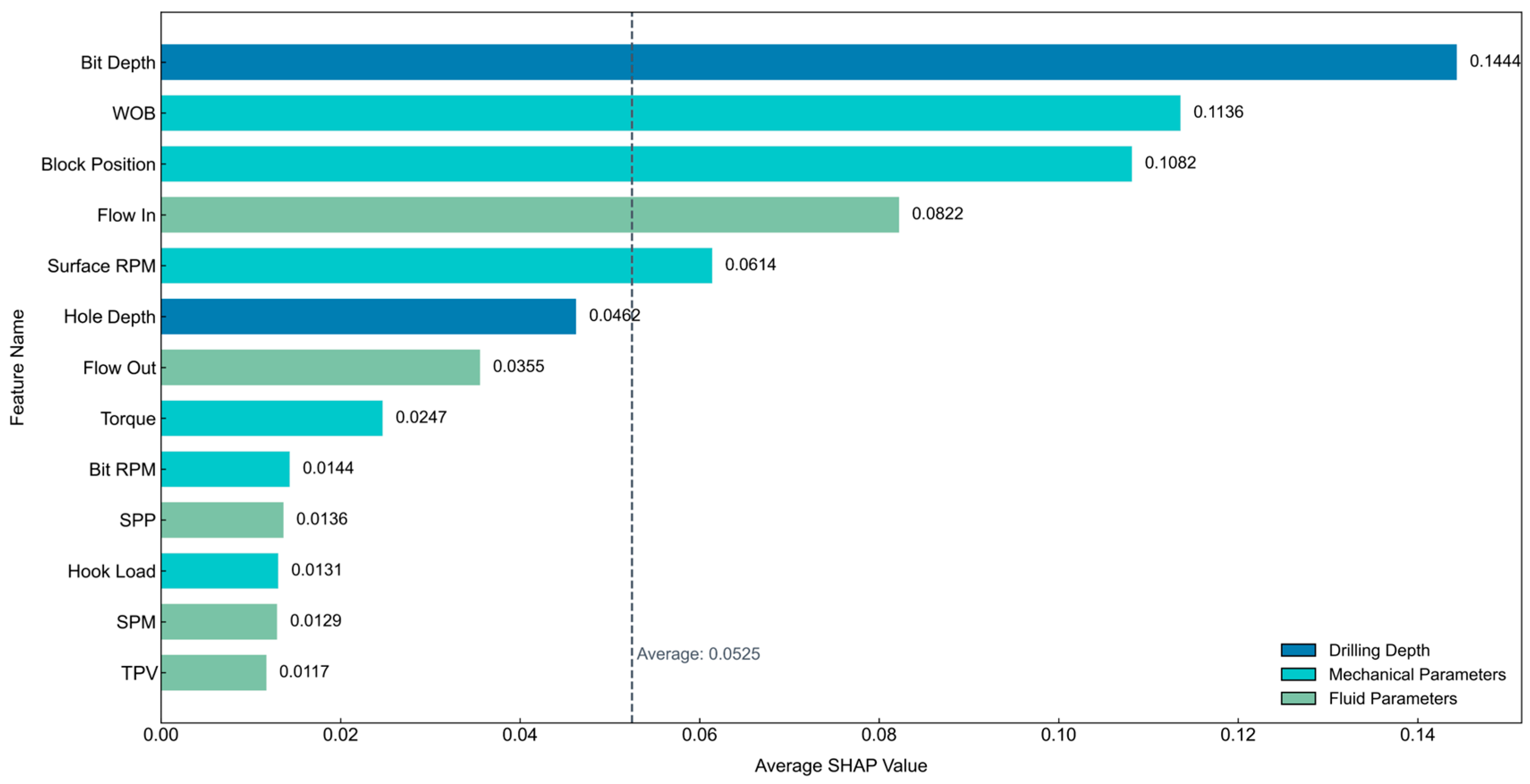
To clarify the relative importance of each input feature in the model’s decision-making process, the SHAP method was employed to quantify feature contributions and reveal the internal reasoning of the deep neural network during drilling operation recognition [43]. As illustrated in Figure 15, the thirteen input variables can be grouped into three categories: mechanical parameters, fluid parameters, and depth parameters.

The ranking of feature importance shows that Bit Depth, WOB, and Block Position have the most significant contributions to operational state recognition. Among them, Bit Depth exhibits the highest importance, indicating that the bit’s position within the wellbore serves as a decisive indicator for operation identification. In practical drilling operations, changes in bit depth directly reflect the working condition: a continuous increase typically corresponds to drilling, while a rapid rise or fall indicates tripping-out or tripping-in operations. The model effectively distinguishes major operational states by capturing these dynamic depth variations.

In addition to Bit Depth, WOB and Block Position play essential supporting roles. WOB reflects the contact force between the bit and the formation, remaining relatively stable during drilling but dropping to zero during tripping or connection operations. Meanwhile, Block Position describes the axial motion of the hoisting system, distinguishing between upward, downward, and static states. Together, these two parameters complement bit depth information and provide the core basis for condition recognition.

Flow In, Surface RPM, and Well Depth contribute at an intermediate level. Flow In represents the circulation status of drilling fluid and is a key indicator for distinguishing between circulating and non-circulating conditions. Surface RPM reflects the rotational motion of the drill string, aiding in differentiating rotating and non-rotating states. Well Depth, when analyzed alongside bit depth, helps determine whether the bit is positioned at the bottom of the well.

Features with relatively lower importance include Flow Out, Torque, Bit RPM, SPP, and Hook Load. Although their overall contribution is limited, they remain crucial in specific operational contexts. Torque variations help differentiate rotary drilling from sliding drilling; the relationship between Bit RPM and Surface RPM indicates potential disconnections within the drill string; while fluctuations in Hook Load provide vital clues during tripping-in, tripping-out, reaming, and back-reaming operations. These parameters, though not primary decision factors, act as complementary indicators for fine-grained state distinctions.

It should be noted that the SHAP-based feature attribution results should be interpreted as model-specific explanatory evidence rather than causal evidence of drilling-state formation. Several drilling parameters are physically coupled and may exhibit strong correlations, such as Bit Depth and Well Depth, as well as Surface RPM and Bit RPM. Such multicollinearity may influence the allocation of SHAP values among correlated variables. Therefore, the feature ranking shown in Figure 15 mainly reflects the relative contribution tendency learned by the present model under the selected background samples, rather than an absolute or unique measure of feature importance.

In summary, the SHAP-based feature attribution results suggest that Bit Depth, WOB, and Block Position play important roles in the model’s classification process. Circulation- and rotation-related parameters provide auxiliary information, while the remaining indicators help improve sensitivity to complex transitional operations. These findings are generally consistent with field engineers’ recognition logic; however, due to possible feature correlations and the dependence of SHAP values on the selected background dataset, the results should be regarded as qualitative interpretability evidence rather than definitive proof of independent feature importance.

4.4.2. Interpretability of the Multi-Head Attention Mechanism

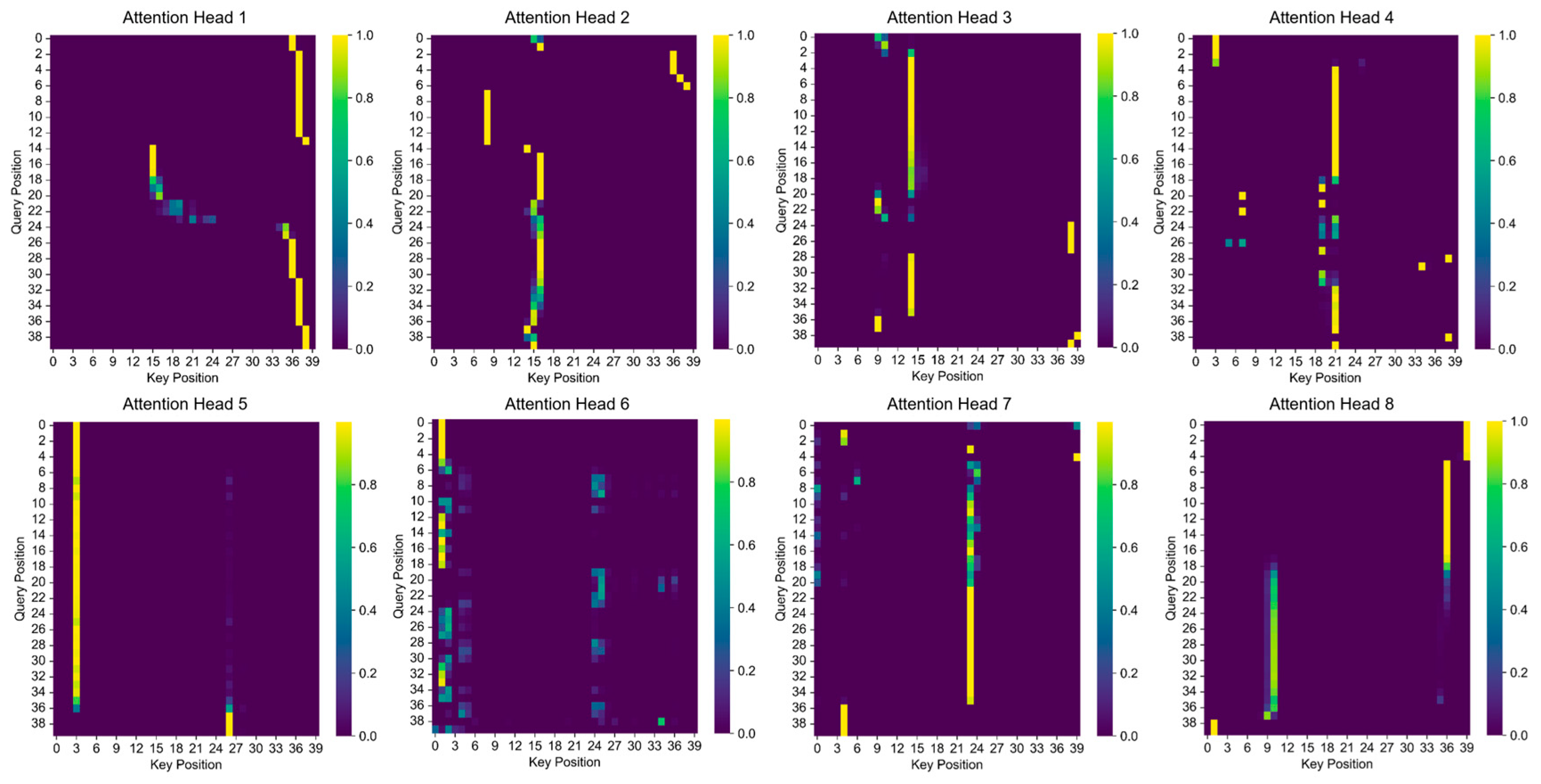
To provide a qualitative interpretation of the multi-head attention mechanism in the drilling operation classification task, the attention weight distributions were visualized and analyzed. As shown in Figure 16, different attention heads exhibit different temporal attention tendencies. For example, the 1st and 8th heads show relatively higher weights near the end of the sequence, suggesting that recent time steps may provide useful information for state recognition. The 2nd to 4th heads tend to assign higher attention to mid-sequence segments, while the 5th and 6th heads show stronger responses at the beginning of the sequence. These observations suggest that the multi-head attention mechanism may capture temporal information from different parts of the input sequence. However, since attention weights are input-dependent and may vary across samples, the visualization should be interpreted as a qualitative indication of temporal attention tendencies rather than as definitive statistical evidence of fixed head-specific specialization.

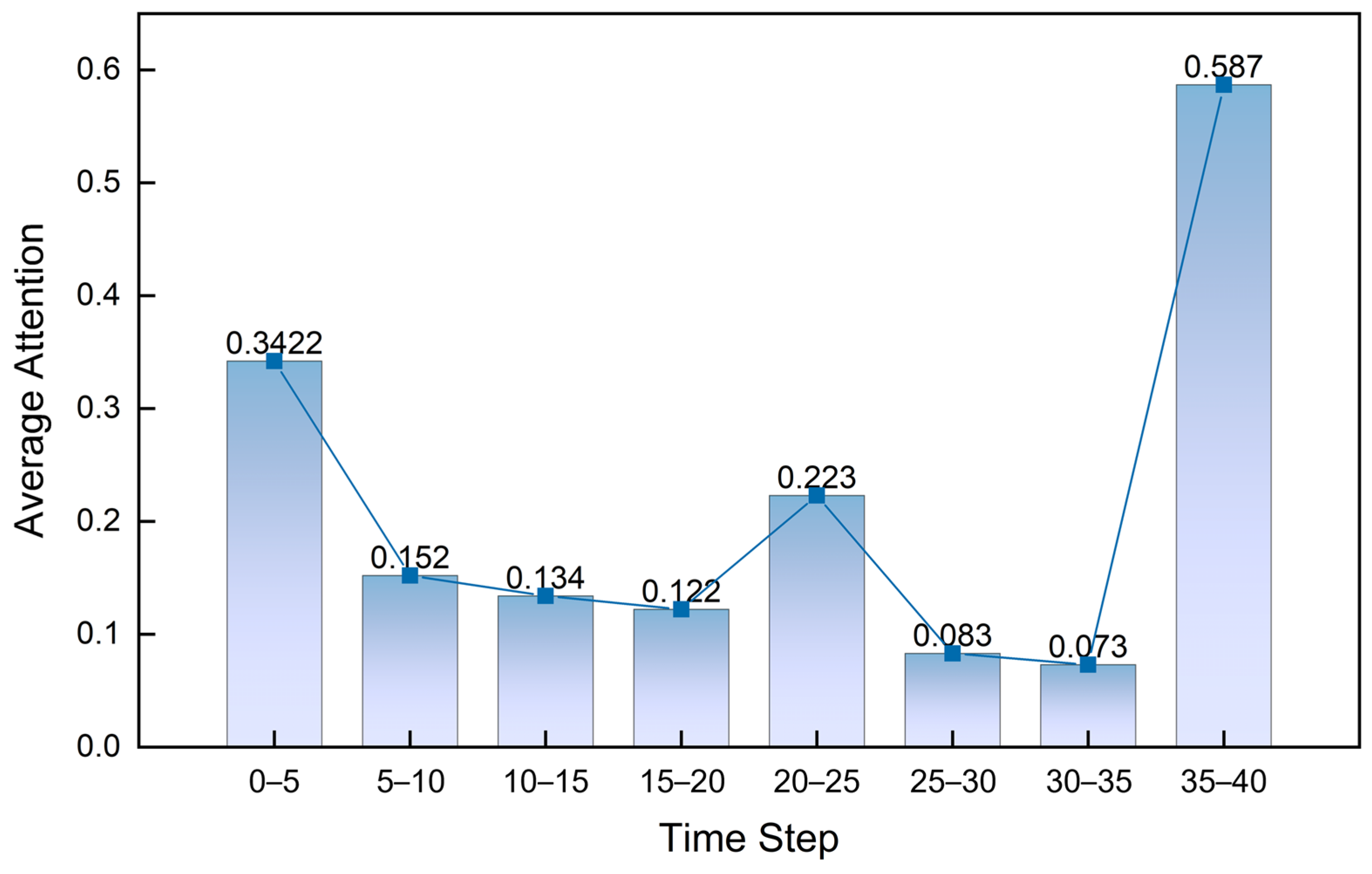
After averaging the attention weights across all heads, the overall temporal distribution is shown in Figure 17. The mean attention value reaches a peak of approximately 0.59 during the final 35–40 time steps, indicating that the model places greater emphasis on recent and instantaneous features when identifying operational states. Attention values in the initial 0–5 steps remain moderately high, around 0.34, suggesting that early contextual cues also support classification. In contrast, the mid-sequence intervals (10–20 and 25–30 steps) display substantially lower weights, below 0.15, with the minimum values, around 0.07, observed between 30 and 35 steps. This pattern implies that mid-range temporal information contributes less to short-term operational state discrimination.

A combined examination of Figure 16 and Figure 17 suggests that the model tends to assign relatively greater attention to recent time steps, while earlier contextual information may also contribute to classification. This tendency is consistent with the practical characteristics of drilling-state recognition, where current operational states are often reflected by short-term variations in key drilling parameters. Nevertheless, the attention maps shown in this section are mainly used as qualitative visualization tools. Because the current analysis does not include the variance, standard deviation, or statistical testing of attention weights across samples, the observed temporal focus patterns should not be interpreted as universal or sample-independent behaviors. A more rigorous assessment of attention consistency across samples will require additional statistical analysis in future work.

4.4.3. Interpretability of Cross-Well Transfer

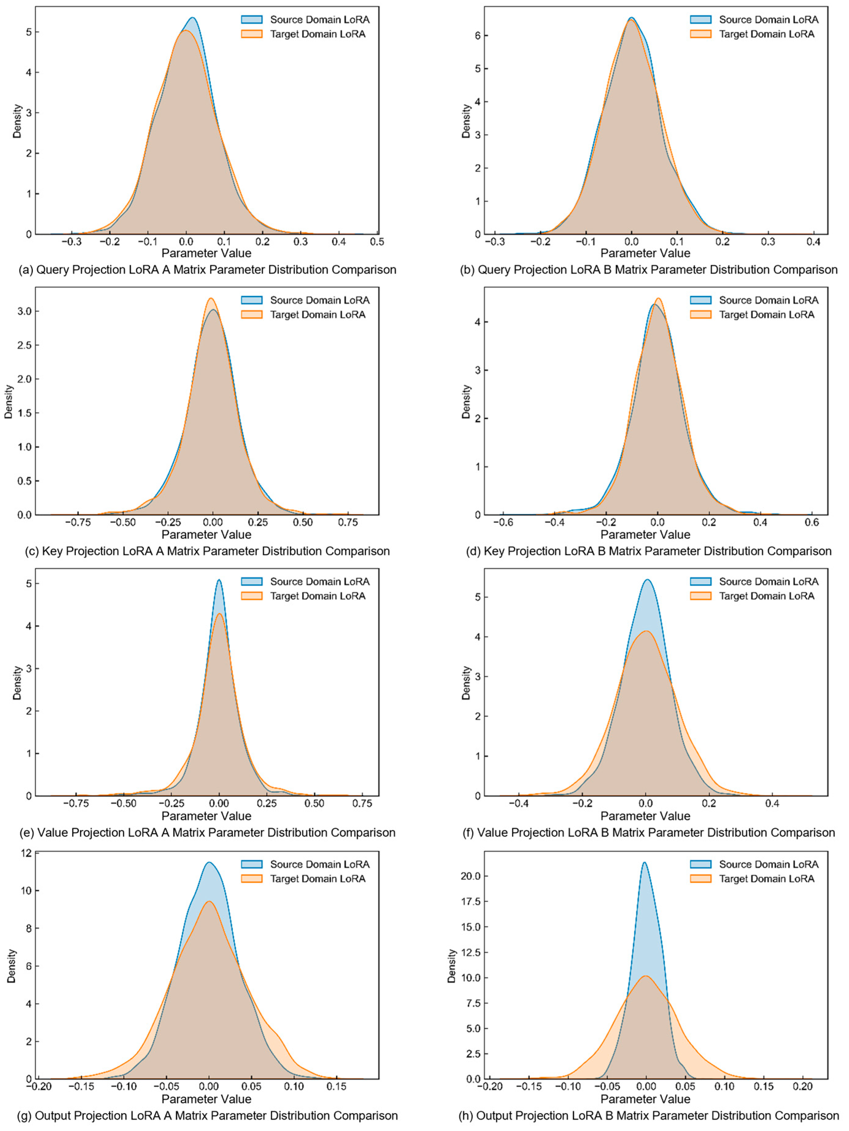
To further clarify the interpretability of cross-well transfer learning, the LoRA parameter distributions of the Query, Key, Value, and Output projection layers were compared between the source and target domains, as illustrated in Figure 18a–f. Distinct parameter shifts were observed in the target domain, with the most significant updates occurring in the Value and Output layers. Specifically, the B matrix exhibited change rates of 27.07% and 118.76%, while the A matrix changed by 20.46% and 29.57%, respectively. These variations reflect differences in data characteristics between drilling sites, suggesting that the model primarily adapts through the Output layer to integrate new domain information, while adjustments in the Value layer help align feature representations with the target domain. In contrast, the Query and Key layers underwent only slight modifications, with change rates ranging from –5% to 4%, indicating that the core attention structure remains largely stable during transfer. Furthermore, both A and B matrices display consistent directional trends across layers, with the B matrix generally showing greater magnitude. This pattern aligns with the LoRA design principle, where the B matrix functions as the expansion component, offering higher flexibility for adaptation and serving as the main contributor to cross-domain parameter updates.

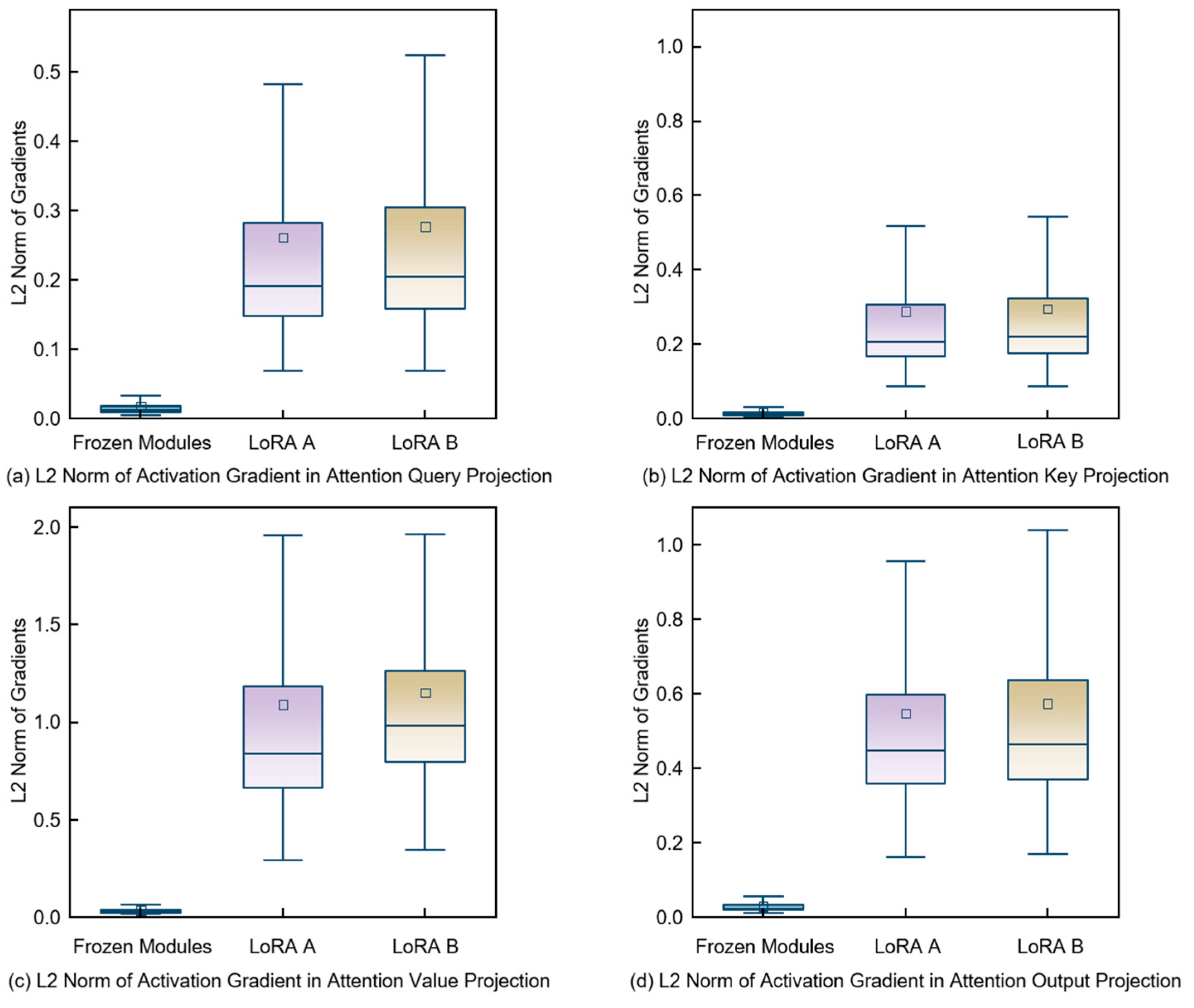
Further insights are provided in Figure 19, which compares the L2 norm distributions of frozen parameters and LoRA adapters (A and B matrices) across the four projection layers. The frozen parameters exhibit small, concentrated gradient magnitudes, reflecting their structural stability and role in retaining foundational feature extraction. The A matrices show moderate, smoothly varying gradients consistent with the frozen layers, suggesting that low-rank decomposition constrains parameter updates, thereby stabilizing the transfer process. The B matrices, however, display significantly larger gradients—particularly in the Value and Output layers—demonstrating their dominant role in domain adaptation by fine-tuning the model to the statistical characteristics of the target well data.

Together, Figure 18 and Figure 19 elucidate the interpretability of the LoRA-based transfer mechanism. The frozen layers preserve core knowledge from the source domain, the A matrices provide directionally consistent constrained updates, and the B matrices perform targeted adaptation in key projection layers. This complementary dynamic enables the model to achieve efficient and interpretable cross-domain transfer, maintaining learned representations while effectively adapting to new well conditions—thereby supporting robust drilling operation recognition across different geological environments.

5. Conclusions

This study addresses three critical challenges in drilling operation state recognition: insufficient temporal dependency modeling, limited cross-well generalization capability, and the lack of model interpretability. To this end, an interpretable deep transfer learning-based approach was proposed. The main conclusions are as follows:

(1)

The proposed MultiHead-BiLSTM model, which integrates a multi-head attention mechanism with a bidirectional LSTM architecture, effectively captures both key transient dynamics and long-term temporal dependencies. This integration improves the model’s ability to distinguish drilling operation states under conditions of blurred operational boundaries and highly similar feature patterns. Experimental results show that the proposed model achieved an accuracy of 95.11% and an F1-score of 94.00% on the test set, achieving the best overall performance among the selected benchmark models, including LSTM, GRU, BiLSTM, and Transformer.

(2)

Within the transfer learning framework, the LoRA-based lightweight fine-tuning strategy enables efficient adaptation to target well data through low-rank parameter decomposition while preserving source domain knowledge. The results indicate that the proposed strategy reduces the cross-well error rate to 1.91%, achieving better transfer performance than direct transfer and partial-layer freezing approaches under the current experimental setting. These findings demonstrate the potential of parameter-efficient adaptation for cross-well drilling-state recognition.

(3)

By combining SHAP feature attribution, attention weight visualization, and LoRA parameter analysis, the proposed framework provides interpretable insights into the model decision-making process. The results suggest that Bit Depth, WOB, and Block Position contribute most significantly to drilling-state recognition, while circulation- and rotation-related parameters provide complementary information. Furthermore, attention visualization indicates that the model focuses on temporal regions associated with operational transitions, and LoRA parameter analysis reveals adaptation characteristics across different projection layers during transfer learning. These analyses improve the transparency and engineering interpretability of the proposed framework.

Despite the encouraging results obtained in this study, several limitations should be acknowledged. The proposed framework was evaluated under specific drilling conditions, and its applicability to more diverse geological settings and operational scenarios requires further investigation. In addition, although the framework demonstrated satisfactory recognition accuracy, transfer capability, and interpretability, its robustness and generalization performance should be further validated across a broader range of drilling environments. Future work will focus on extending the evaluation of the proposed framework to more diverse drilling datasets and operational conditions, exploring advanced sequence-modeling and transfer learning techniques, and further enhancing the robustness, adaptability, and interpretability of intelligent drilling-state recognition systems.