Article

Analysis and Suppression of Torsional Vibration with Coordinated Control for Integrated Electric Drive Systems of Electric Vehicles


1
School of Automotive and Information Engineering, Guangxi Eco-Engineering Vocational and Technical College, Liuzhou 545006, China
2
Mechanical and Automotive Engineering School, Guangxi University of Science and Technology, Liuzhou 545006, China
3
School of Automotive and Traffic Engineering, Guangxi Electrical Polytechnic Institute, Nanning 530007, China
4
School of Automotive Engineering, Liuzhou Institute of Technology, Liuzhou 545006, China
*
Authors to whom correspondence should be addressed.
Processes 2026, 14(12), 1929; https://doi.org/10.3390/pr14121929
Submission received: 11 April 2026 / Revised: 3 June 2026 / Accepted: 11 June 2026 / Published: 13 June 2026
(This article belongs to the Section Automation Control Systems)

Abstract

Aiming at the deterioration in Noise, Vibration and Harshness (NVH) performance caused by broadband torsional vibration in the integrated electric drive system (IEDS) of electric vehicles, most existing studies independently focus on electromagnetic excitation suppression or torsional vibration control of mechanical transmissions. Few researchers consider the coupling characteristics between the electromagnetic nonlinearity of motors and the nonlinearity of gear transmissions, making it difficult to realize the coordinated suppression of high- and low-frequency torsional vibration. In this paper, a seven-degree-of-freedom electromechanical coupling dynamic model is firstly established, which incorporates the electromagnetic torque ripple of the motor, the time-varying meshing stiffness of gears, meshing errors, and gear backlash nonlinearity. Through modal analysis and Campbell diagram solution, the natural characteristics and critical speed range of the system are clarified, and the generation mechanism of full-frequency band torsional vibration as well as the high–low frequency coupling characteristics are systematically revealed. On this basis, a coordinated active control strategy based on PD pole placement and harmonic current injection (PD-HCI) is proposed. The PD pole placement controller is adopted to suppress the low-frequency torsional vibration (0–20 Hz) of the transmission system, and the 5th/7th harmonic current injection is used to counteract the high-frequency torque ripple (above 200 Hz) of the motor, thereby achieving the coordinated suppression of broadband torsional vibration. The Matlab/Simulink R2023a simulation results show that the proposed control strategy reduces the torque fluctuation rate from 3.11% to 1.96%, the speed fluctuation rate from 0.10% to 0.03%, and the total harmonic distortion (THD) of stator current from 8.69% to 1.77% under steady-state operating conditions. Under transient operating conditions with sudden load changes, the stabilization time of fluctuations in speed and half-shaft torque is shortened by more than 80%, the impact amplitude is significantly reduced, and there is no loss in the vehicle’s dynamic response and speed tracking performance. Experimental results show that the coefficients of determination R2 of vehicle speed, motor speed, acceleration and torque are 0.9990, 0.9982, 0.9997 and 0.9997, respectively, which verifies the reliability of the established model.

1. Introduction

With the increasingly severe global energy crisis and environmental pollution issues, electric vehicles (EVs), as an ideal alternative to traditional fuel vehicles, have become a key development direction of the automotive industry [1]. The integrated electric drive system (IEDS) has been widely adopted in modern electric vehicles due to its advantages such as compact structural design, high power density, and high transmission efficiency [2]. The IEDS generally integrates key components, including the drive motor, reducer, and differential, into a single assembly. This structure effectively reduces the power transmission links and improves the vehicle space utilization and energy conversion efficiency [3,4]. However, while the integrated design provides numerous advantages, it also introduces new Noise, Vibration and Harshness (NVH) issues [5]. Since electric vehicles lack the noise masking effect of traditional internal combustion engines, the vibration and noise problems of the electric drive system become more prominent, which directly affects ride comfort and vehicle quality [6,7]. Relevant studies indicate that the vibration problems in the IEDS can be mainly divided into two categories: low-frequency torsional vibration (0–20 Hz) and high-frequency torsional vibration (200–20,000 Hz) [8]. Low-frequency torsional vibration is mainly caused by the elastic characteristics of the drive shaft [9], whereas high-frequency torsional vibration is primarily induced by motor torque ripple and gear backlash [10]. At present, extensive research on the NVH control of the IEDS has been conducted by scholars worldwide, which is mainly carried out from two aspects: passive control and active control [11].
Research on passive control mainly suppresses vibration excitation sources or optimizes vibration transmission paths through structural and parametric optimization, serving as a fundamental method for the vibration control of the IEDS. Existing studies focus primarily on two categories: motor structure optimization and gear transmission system optimization [12]. In the field of motor structural optimization, relevant studies generally suppress cogging torque and electromagnetic torque ripple by adjusting air-gap length and permanent magnet parameters, as well as adopting skewed slot and skewed pole designs [13]. Ocak et al. proposed a stepwise skewed pole method with variable magnetic poles based on semi-finite element analysis, which minimizes cogging torque and torque ripple by optimizing the number of rotor segments [14]. Katona et al. systematically reviewed the torque ripple suppression technologies for permanent magnet synchronous motors and clarified the dominant influencing mechanisms of electromagnetic disturbances, including cogging torque, reluctance torque fluctuation, and permanent magnet torque fluctuation [15]. Focusing on axial-flux permanent magnet motors, Pranjić et al. summarized cogging torque suppression schemes, such as pole shifting, stator slot opening optimization, and permanent magnet shape design, and verified the suppression effect of pole shifting and slot opening optimization on air-gap magnetic field harmonics [16]. Shi et al. pointed out that although skewed slot design is one of the most widely adopted NVH control strategies for vibration reduction, it has limitations such as reduced output torque and increased manufacturing cost [17]. In the field of gear transmission system optimization, research focuses on tooth profile design, meshing characteristic optimization, and nonlinear backlash control. Pleguezuelos et al. established analytical models of meshing stiffness, load distribution and transmission error for profile-modified spur gears under off-nominal loads, providing a theoretical tool for gear parameter optimization [18]. Hou et al. clarified that gear transmission error is the primary excitation of gear whine and verified that micro-tooth profile optimization can minimize transmission error [19]. Liao et al. revealed the influence law of backlash and bearing clearance nonlinearity on the torsional vibration of gear transmission systems [20]. Faysal introduced time-varying meshing stiffness into the NVH system model and proposed a dynamic simulation method for gear meshing under wide operating conditions, providing simulation support for the NVH optimization of gear systems [21].
Research on active control has formed four major core technical approaches. The first category refers to control methods based on reference torque optimization, which suppress torsional vibration by modifying the reference torque commands of the motor. Focusing on torque fluctuations induced by magnetic flux harmonics, Shuang et al. proposed an active torsional vibration suppression method based on the analytical calculation of optimal harmonic current commands [22]. Zhang et al. developed an active torsional vibration suppression strategy based on dual-loop control for the powertrain of power-split hybrid electric vehicles. By real-time vibration signal processing and adaptive compensation torque calculation, the strategy effectively suppresses low-frequency torsional vibration and realizes real-time torque compensation via feedback controllers [23]. The second category is the harmonic injection method, which counteracts torque ripple by injecting specified harmonic components into the motor current and is currently the most widely applied active control approach. Qu et al. adopted an iterative learning control strategy to optimize the amplitude and phase of harmonic currents and proposed a novel torque ripple suppression method based on advanced harmonic current control [24]. Yi et al. systematically reviewed torque ripple minimization technologies based on harmonic injection and compared the control principles and performance of various injection strategies [25]. Considering DC bus voltage constraints, Wu and Lyu further optimized the d-axis harmonic current injection strategy to achieve optimal harmonic injection and torque ripple suppression within voltage limits [26]. Dai et al. proposed a data-driven current harmonic optimization method, established a metamodel relating injected harmonics, torque ripple and system losses, and achieved multi-objective collaborative optimization [27]. The third category is vibration control based on Quasi-Zero Stiffness (QZS) isolators. By parallel arrangement of positive and negative stiffness, such isolators achieve high static stiffness and low dynamic stiffness, showing prominent advantages in low-frequency vibration isolation. Xu et al. designed a QZS joint actuator, derived analytical expressions for force and torque transmissibility, and verified its excellent vibration isolation performance [28]. Sun et al. proposed an active gravity compensation control method for QZS isolators under variable loads, which effectively improves the operating condition adaptability of vibration isolation systems [29]. Chen et al. combined the QZS structure with air suspensions, designed H2/H∞ state-feedback semi-active controllers and polynomial chaos expansion-based robust controllers, and greatly enhanced the vibration isolation performance and robustness of suspension systems [30]. Tuo et al. developed an integrated seat suspension with QZS vibration isolation and energy harvesting, realizing the coordination of vibration suppression and energy recovery [31]. The last category is shaft torque feedback control, which suppresses torsional vibration through real-time monitoring and feedback compensation of drive shaft torque. Sun et al. proposed an active torsional vibration suppression method for IEDS considering nonlinear factors, which synchronously suppresses both low- and high-frequency torsional vibration by optimizing harmonic current commands [32]. For dual-motor drive systems, Yue et al. proposed a real-time self-tuning active control strategy combined with fuzzy control theory [33]. Aiming at the backlash nonlinear effect under low-speed conditions, Jiang et al. realized effective suppression of low-speed driveline vibration via damping torque estimation [34]. Recent vehicle-level studies on distributed-drive electric vehicles have further emphasized that electric-drive control should coordinate stability, energy consumption and actuator allocation under changing driving events [35], which motivates the development of vibration suppression strategies that maintain vehicle dynamic performance while improving NVH behavior.
In summary, most existing studies seldom consider the coupling relationship between the motor electromagnetic torque and the mechanical transmission system. Addressing the above research gaps, this paper takes the integrated electric drive system (IEDS) of electric vehicles as the research object. Firstly, a refined electromechanical coupling dynamic model considering both motor electromagnetic nonlinearity and gear transmission nonlinearity is established to systematically reveal the generation mechanism of full-band torsional vibration and the high–low frequency coupling characteristics in the IEDS. On this basis, a coordinated active control strategy with multi-source excitation is proposed, which balances the motor dynamic performance and full-band vibration suppression.

2. Natural and Nonlinear Characteristics of the IEDS

The IEDS investigated in this paper is shown in Figure 1. The development of the simulation model lays a solid foundation for the subsequent design of control strategies.

2.1. Motor Model

The Interior Permanent Magnet Synchronous Motor (IPMSM) is a nonlinear and strongly coupled system with high-frequency fluctuations in its output torque. To facilitate analysis and control design, the following assumptions are adopted: the iron core saturation effect, eddy current loss, and hysteresis loss are neglected; temperature variations and material characteristic drift are not considered. Meanwhile, a flux linkage model is employed to describe the relationship between voltage and current, as expressed in the following equation:
  u d = R s i d + d ψ d d t ω e ψ q u q = R s i q + d ψ q d t ω e ψ d
where ωe denotes the electrical angular velocity, Rs is the stator resistance, and ψd and ψq represent the d-axis and q-axis flux linkages, respectively.
The flux linkage equations are given as follows:
ψ d = L d i d + ψ f ψ q = L q i q
In an actual motor control system, the stator windings of an IPMSM are mainly connected in a star configuration. Under ideal conditions, the windings are symmetrically distributed, and the back electromotive force (back EMF) waveform of the windings contains no even-order harmonics. Accordingly, the dominant harmonic components of the three-phase stator current are the fifth, seventh, 11th and 13th harmonics, among which the fifth and seventh harmonics have the highest content. When harmonic components are considered, the three-phase stator current of the motor can be expressed as:
i a = i 1 sin ( ω t + θ 1 ) + i 5 t h sin ( 5 ω t + θ 2 ) + i 7 t h sin ( 7 ω t + θ 3 ) i b = i 1 sin ω t + θ 1 2 π 3 + i 5 t h sin 5 ω t + θ 2 2 π 3 + i 7 t h sin 7 ω t + θ 3 2 π 3 i c = i 1 sin ω t + θ 1 4 π 3 + i 5 t h sin 5 ω t + θ 2 4 π 3 + i 7 t h sin 7 ω t + θ 3 4 π 3
where i1, i5th, and i7th are the amplitudes of the fundamental current, fifth harmonic current, and seventh harmonic current, respectively, and θ1, θ2, and θ3 are the initial phase angles of the fundamental current, fifth harmonic current, and seventh harmonic current, respectively.
Under the constraint of constant amplitude, the three-phase stator currents are transformed into the dq reference frame:
i d   = i d 1 + i 5 t h cos ( 6 ω t + θ 5 ) + i 7 t h cos ( 6 ω t + θ 7 ) i q   = i q 1 + i 5 t h sin ( 6 ω t + θ 5 ) + i 7 t h sin ( 6 ω t + θ 7 )
where id1 and iq1 are the d-axis and q-axis components of the fundamental current, respectively, and θ5 and θ7 are the initial phase angles of the fifth and seventh harmonic currents, respectively.
The torque equation of the IPMSM is given as follows:
T e = 3 2 P n ( ψ f i q + ( L d L q ) i q i d )
where Pn is the number of pole pairs.
The dynamic equation of the motor is given as follows:
I m d ω m d t = T e T L B ω m
where Im is the moment of inertia, B is the viscous damping coefficient, TL is the load torque, and ωm is the mechanical angular velocity of the motor. The parameters of the IPMSM are listed in Table 1.

2.2. Gear Transmission System Model

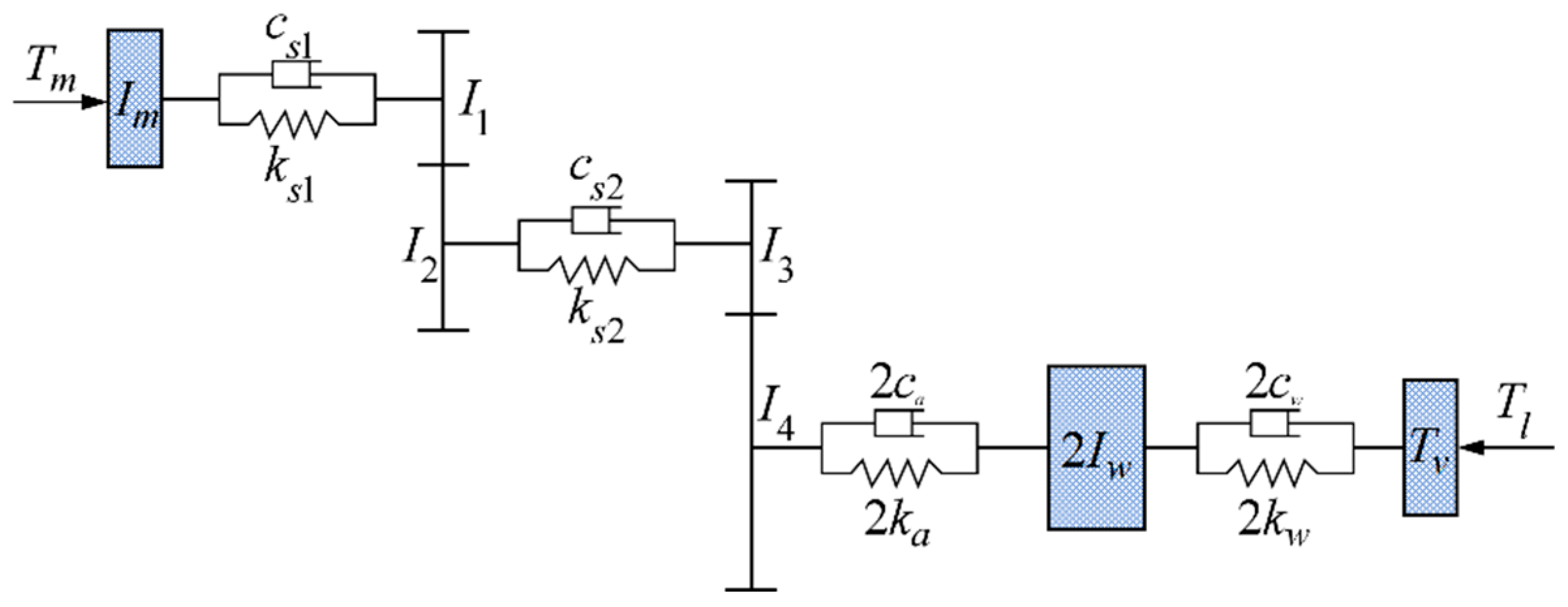
The output shaft of the IPMSM is rigidly connected coaxially with the input shaft of the transmission system via splines, and the transmission system adopts a two-stage helical gear reducer. The output torque of the motor is decelerated by the two-stage gears and then transmitted to the left and right wheels through the differential to drive the battery electric vehicle. Each shaft is equivalent to an elastic shaft considering stiffness and damping, while the drive motor, gears, wheels and vehicle body are equivalent to lumped masses with moments of inertia. Taking gear meshing dynamics into account simultaneously, a pure torsional dynamic model of the powertrain system is established, as shown in Figure 2.
The reason for adopting a pure torsional representation is that the main concern of this study is the rotational vibration transmitted along the motor–reducer–half-shaft torque path. In this path, the dominant resonance behavior is governed primarily by the equivalent inertias, shaft stiffness, shaft damping and gear-meshing excitations; therefore, the model retains the rotational degrees of freedom of the motor, gears, wheels and equivalent vehicle while incorporating time-varying meshing stiffness, meshing error and backlash. The model is not intended to describe bearing flexibility, housing vibration or axial/lateral gear modes. Instead, it is used to capture the dominant torsional resonance, half-shaft torque fluctuation and motor-speed oscillation that directly affect IEDS NVH performance.
Based on Newton’s second law, a seven-degree-of-freedom pure torsional dynamics model for a two-stage bevel gear transmission system is established:
I m θ ¨ m + k s 1 ( θ m θ 1 ) + c s 1 ( θ ˙ m θ ˙ 1 ) = T m I 1 θ ¨ 1 + k s 1 ( θ 1 θ m ) + c s 1 ( θ ˙ 1 θ ˙ m ) = 0 I 2 θ ¨ 2 r 2 F m 1 + k s 2 ( θ 2 θ 3 ) + c s 2 ( θ ˙ 2 θ ˙ 3 ) = 0 I 3 θ ¨ 3 + k s 2 ( θ 3 θ 2 ) + c s 2 ( θ ˙ 3 θ ˙ 2 ) + r 3 F m 2 = 0 I 4 θ ¨ 4 r 4 F m 2 + 2 k a ( θ 4 θ w ) + 2 c a ( θ ˙ 4 θ ˙ w ) = 0 I w θ ¨ w k a ( θ 4 θ w ) c a ( θ ˙ 4 θ ˙ w ) + k w ( θ w θ v ) + c w ( θ ˙ w θ ˙ v ) = 0 I v θ ¨ v 2 k w ( θ w θ v ) 2 c w ( θ ˙ w θ ˙ v ) + T l = 0
where Tm denotes the electromagnetic torque; θm, θ1, θ2, θ3, θ4, θw, and θv represent the rotation angles of the motor shaft, the driving gear of the first-stage gear pair, the driven gear of the first-stage gear pair, the driving gear of the second-stage gear pair, the driven gear of the second-stage gear pair, the wheel, and the equivalent vehicle, respectively; and Tl represents the driving resistance torque of the vehicle, which is calculated by the following equation:
T l = ( m g f cos α + m g sin α + C d A ( v + v w ) 2 21.15 + δ m d v d t ) r
where Tl represents the driving resistance torque of the vehicle. The definitions and values of the other main parameters are listed in Table 2.
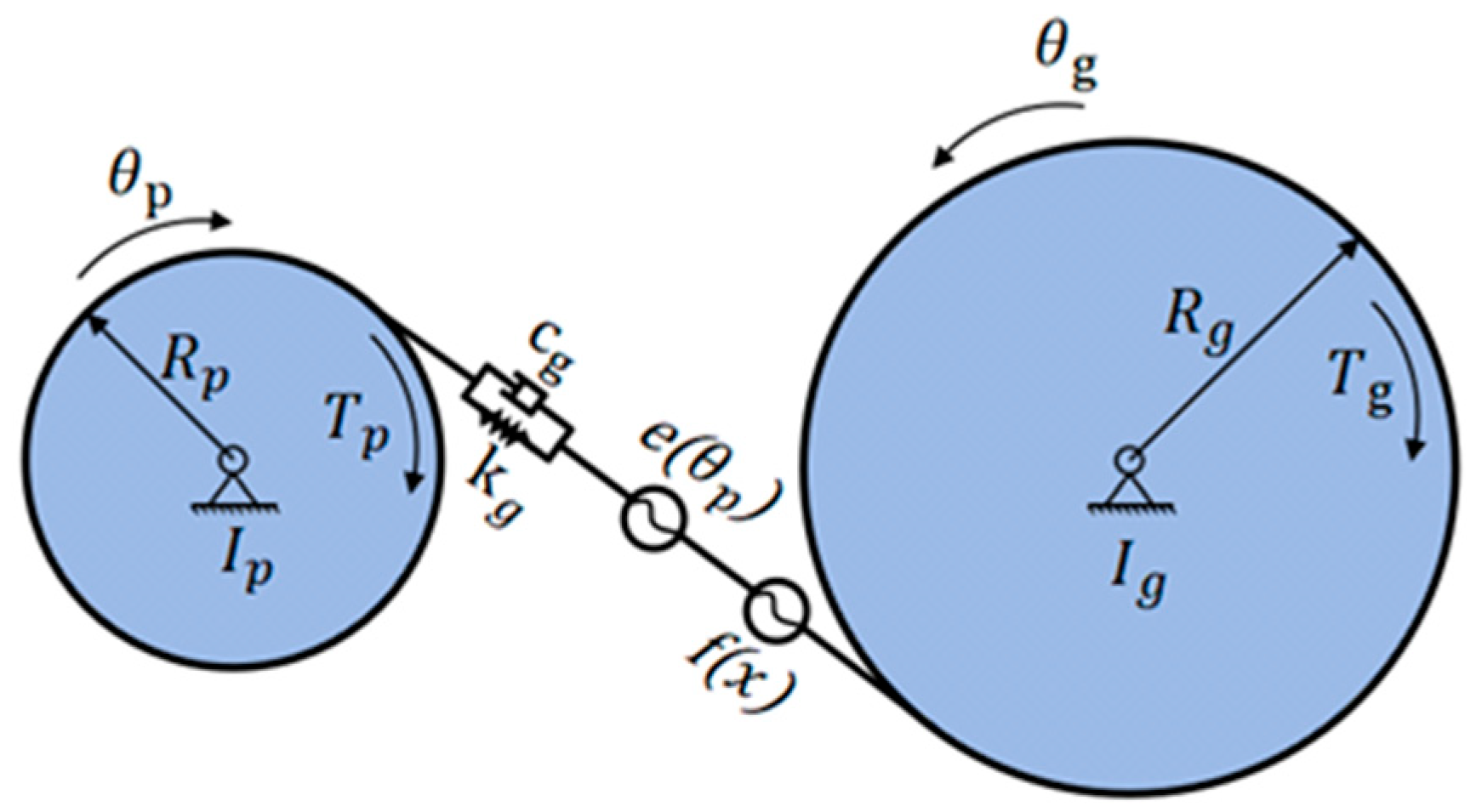
To balance transmission smoothness and structural integration, cylindrical helical gear pairs are commonly adopted for the two-stage final drive in electric drive systems. On the premise of neglecting the elastic deformation of bearings and the slight transverse and longitudinal vibrations of gears, nonlinear excitations such as time-varying meshing stiffness, backlash and meshing error are incorporated, and a pure torsional dynamic model is established, as shown in Figure 3.
Considering the above meshing nonlinear excitations, the meshing force between the driving and driven gears can be calculated by the following equation:
F m = k g ( θ p ) f [ cos β ( R p θ p R g θ g ) e ( θ p ) ] + c g [ cos β ( R p θ ˙ p R g θ ˙ g ) e ˙ ( θ p ) ]
where Ip and Ig denote the moment of inertia of the driving and driven gears; Rp and Rg represent the base circle radius of the driving and driven gears; θp and θg are the rotation angles of the driving and driven gears; cg is the meshing damping; kg(θp) and e(θp) represent the time-varying meshing stiffness and meshing error, respectively; f(x) is the backlash function; and x denotes the relative displacement. The notation θp is used consistently as the independent variable for both the stiffness and error functions in Equations (9) and (10). The parameters of the gear pairs in the two-stage final drive in this paper are listed in Table 3.
(1)
Time-varying meshing stiffness.
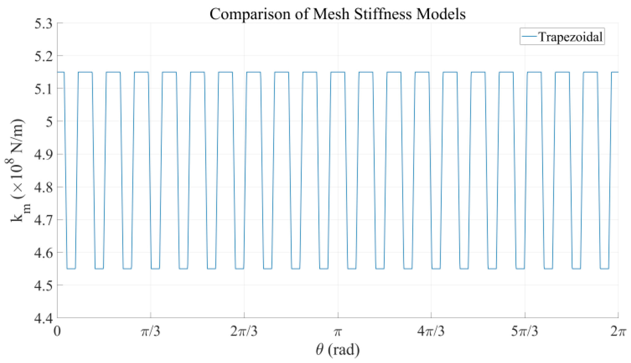
During the gear meshing process, the gear teeth undergo elastic deformation under load, and the ability to resist such deformation is defined as meshing stiffness. Due to the periodic variation in the number of tooth pairs simultaneously engaged in meshing, the elastic deformation of gear teeth also changes periodically, resulting in time-varying meshing stiffness. This time-varying stiffness causes dynamic fluctuations in the meshing force and is one of the main internal excitations that induce torsional vibration in the transmission system. The average time-varying stiffness is shown in Figure 4.
(2)
Meshing error.
Due to manufacturing limitations, errors are inevitable in gears, causing the gear teeth to deviate from the theoretical meshing position and resulting in fluctuations in the instantaneous transmission ratio, which serves as a type of internal excitation for the transmission system. Pitch deviation, profile deviation, tooth form deviation and other gear errors are generally lumped into a single meshing error, which is represented by a simple harmonic function, as shown in the following equation:
e ( θ p ) = e m + e 0 sin ( z p θ p + φ )
where em denotes the average meshing error and is generally assigned a value of 0, and e0 represents the amplitude of the total tangential composite deviation, which can be determined from GB/T 10095.1-2008 according to the gear accuracy grade. The gear accuracy grade adopted in this paper is Grade 5. According to the standard, the amplitude of the total tangential composite deviation for the first-stage gear pair is 6 µm, and that for the second-stage gear pair is 8 µm. φ is the initial phase angle, which is generally set to 0.
(3)
Gear backlash.
In actual machining, backlash must be reserved on the non-working side of gears to maintain lubrication and compensate for the adverse effects of manufacturing errors, assembly errors and thermal deformation. The corresponding backlash function is expressed by the following equation:
f ( x ) = x b , x > b 0 , x < b x + b , x < b
where b denotes half of the gear backlash and x represents the relative displacement at the gear meshing point, as shown in the following equation:
x = cos β ( R p θ p R g θ g ) e ( θ p )

2.3. Effects of Natural Frequency and Nonlinear Excitation on Torsional Vibration

(1)
Influence of Natural Frequency.
When external excitation is applied to the system, the dynamic response of the system mainly depends on its inherent properties. To accurately identify the characteristics of the external excitation, the inherent characteristics of the system need to be obtained by solving the characteristic equation. The dynamic equation of the system is given as follows:
M X ¨ + K X = 0 M 1 K ω n 2 E = 0
where M is the inertia matrix, X is the displacement matrix, and K is the stiffness matrix.
The harmonic torque components in the electromagnetic excitation spectrum of an IPMSM act as the initial disturbance source. Since their frequency-domain characteristics are close to the modal frequencies of the transmission system, they induce a resonant response of the system. This resonance is amplified through the mechanical transmission path, resulting in a significant increase in the amplitude of the shaft dynamic load. The harmonic frequency of the motor torque ripple is positively correlated with the motor speed; as the speed increases, the harmonic frequency gradually rises. When the speed reaches a specific value, the harmonic frequency of the torque ripple coincides exactly with the natural frequency of the transmission system, and this speed is referred to as the critical speed. When the transmission system operates at the critical speed, the resonance effect is triggered, causing severe system vibration. The critical speed can be calculated using the following formula:
n * = 60 f n r P n
Therefore, the natural frequencies of the system can be obtained as listed in Table 4.
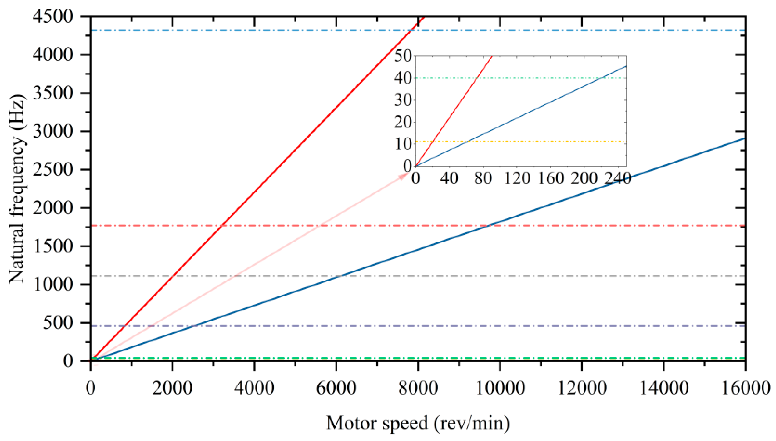
The EDS Campbell diagram is shown in Figure 5. The first- to sixth-order natural frequencies (the horizontal dashed lines from bottom to top correspond to 11.28 Hz, 40.07 Hz, 458.92 Hz, 1114.69 Hz, 1771.65 Hz and 4319.99 Hz, respectively) are represented by dashed lines, while the 11th- and 34th-order electromagnetic force waves are depicted by blue and red solid lines, respectively. The intersection points of the two are the locations of critical speeds. Under low-speed driving conditions, the resonant vibration effect of the system is mainly concentrated at low-order natural frequencies (near 11.28 Hz and 40.07 Hz), which is mainly manifested as low-frequency jitter and rumbling. The 11th-order electromagnetic force wave intersects the first two order natural frequencies at 61.53 rpm and 218.56 rpm, respectively, while the 34th-order harmonic coincides with the low-order natural frequencies at 19.90 rpm and 70.72 rpm. Under medium- and high-speed conditions, the 11th-order electromagnetic force wave coincides with the third-, fourth- and fifth-order natural frequencies at 2503.20 rpm, 6080.13 rpm and 9663.55 rpm, respectively; the 34th-order harmonic coincides with the third-, fourth-, fifth- and sixth-order natural frequencies at 809.27 rpm, 1967.10 rpm, 3126.44 rpm and 7828.73 rpm, respectively. These operating conditions will cause the stator housing and reducer gears to bear large dynamic loads. To avoid resonance risks, measures should be taken to adjust the position of the resonance band so as to reduce the excitation effect of natural frequencies on the electric drive system.
(2)
Influence of Time-varying Meshing Stiffness.
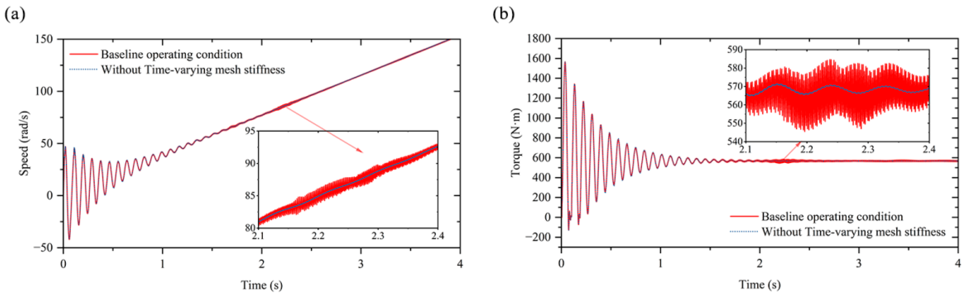
As shown in Figure 6a, time-varying mesh stiffness (TVMS) exerts a significant modulation effect on the dynamic response of the transmission system. As illustrated in the left part of the figure, within the locally amplified interval of the motor shaft speed response (2.1–2.4 s), the baseline case considering TVMS (red solid line) exhibits distinct periodic sawtooth fluctuations with an amplitude of approximately ±2–3 rad/s, superimposed on the macroscopic upward speed trend. In contrast, the comparison case neglecting TVMS (dashed line) shows a smooth, monotonically increasing curve with almost no high-frequency fluctuation components. As depicted in Figure 6b, the influence of TVMS on load transmission characteristics is even more pronounced. During the period of 2.1–2.4 s after the system reaches steady state, the torque curve with TVMS considered (red solid line) presents high-frequency oscillations around the mean value (about 565 N·m), with a peak-to-peak value of 40–50 N·m and a fluctuation rate of approximately ±4%. The case without considering TVMS, however, displays an almost constant steady-state torque (about 570 N·m), and its dynamic fluctuation is negligible.
(3)
Influence of Meshing Error.
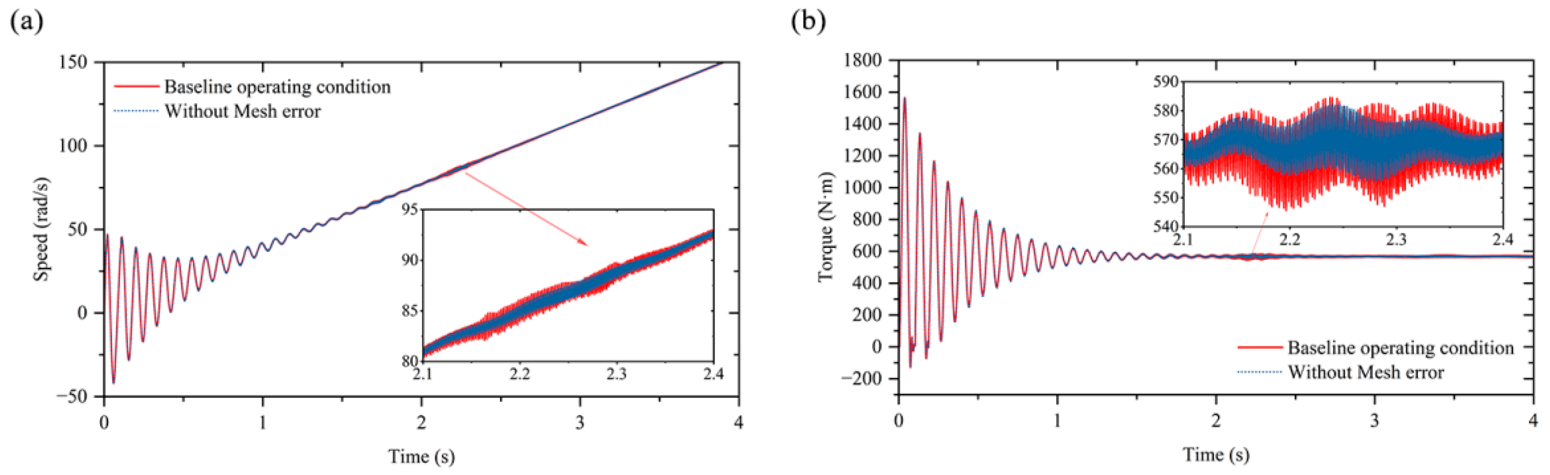
As shown in Figure 7a, gear mesh error exerts a significant modulation effect on the dynamic response of the transmission system, and its influence mechanism is fundamentally different from that of time-varying stiffness excitation. As illustrated in the locally amplified region of the motor shaft speed response on the left (2.1–2.4 s), the baseline case considering mesh error (red solid line) shows distinct low-frequency beat vibration characteristics, whose envelope frequency is consistent with the gear rotational frequency (or error order). The fluctuation amplitude is significantly higher than that of the ideal case without mesh error (dashed line). This low-frequency modulation phenomenon originates from displacement-type excitation caused by geometric eccentricity or profile deviation. As depicted in Figure 7b, the influence of mesh error on load transmission stability is more prominent. During the steady-state operating period (2.1–2.4 s), the torque curve with mesh error considered (red solid line) exhibits low-frequency, large-amplitude fluctuations within a range of approximately 540–590 N·m, accompanied by an obvious trend drift. In contrast, the torque curve without considering mesh error (dashed line) shows a reduced fluctuation range of about 550–580 N·m.
(4)
Influence of Gear Backlash.
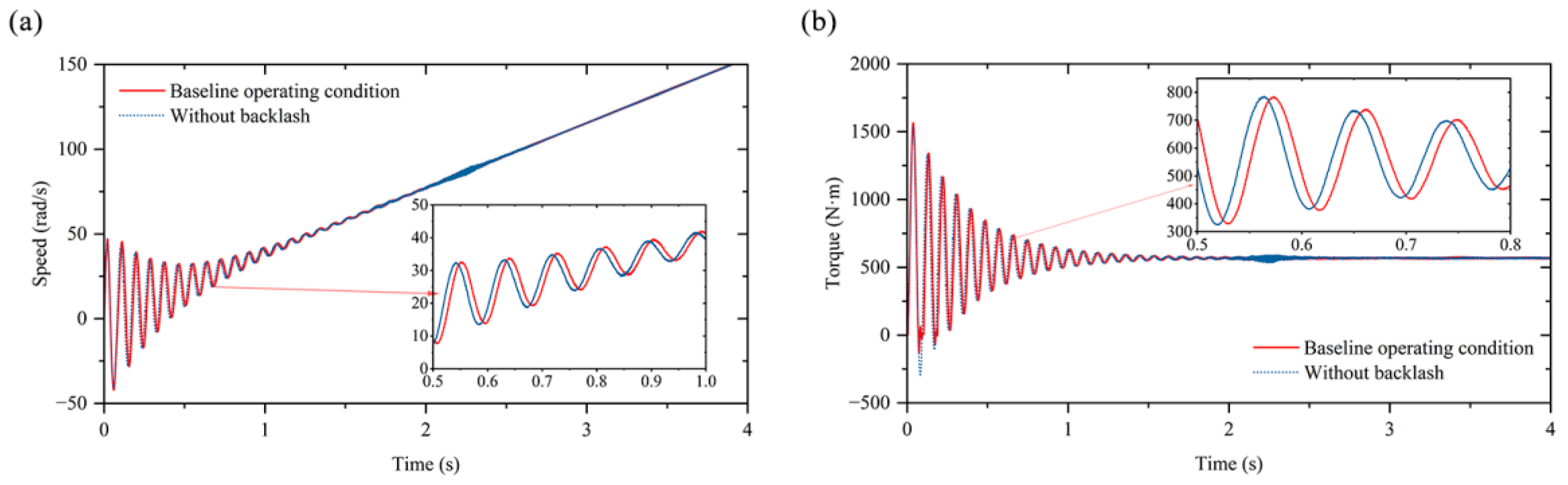
Gear backlash, an inherent nonlinear characteristic of gear transmission systems, exerts a significant dual influence on transmission performance. As shown in Figure 8a,b, the presence of backlash introduces obvious transmission delay and dynamic oscillation in the motor shaft speed response. Compared with the smooth exponential convergence characteristic under the ideal backlash-free condition, the speed curve of the system with backlash exhibits distinct phase lag and high-frequency sawtooth fluctuations. This is because the driving gear must first complete the lost motion to eliminate the backlash before driving the driven gear, resulting in “dead time” during motion transmission. However, from the perspective of engineering feasibility, completely eliminating backlash is neither realistic nor desirable. Without sufficient backlash allowance, tooth surface seizing or scuffing failure will occur.
The effects of parameter uncertainties can also be interpreted from the nonlinear terms retained in the model. Shaft stiffness uncertainty mainly changes the equivalent natural frequencies and thus shifts the resonance-speed range; damping uncertainty changes the decay rate and peak amplification of torsional oscillation; load torque variation enters the system as an external disturbance and changes both the steady torque level and transient impact amplitude; and backlash uncertainty modifies the dead-zone width in f(x), thereby affecting the impact response and phase lag during torque reversal. Therefore, these quantities are not treated as negligible factors. They are included in the mechanism model as the principal sources that determine resonance position, transient overshoot and residual torque ripple.

3. Research on Active Vibration Suppression Based on Harmonic Current Injection and PD Pole Placement

3.1. Harmonic Current Injection (HCI)

The current harmonic suppression method is composed of two components: current harmonic extraction and harmonic compensation voltage calculation.
(1)
Current Harmonic Extraction.
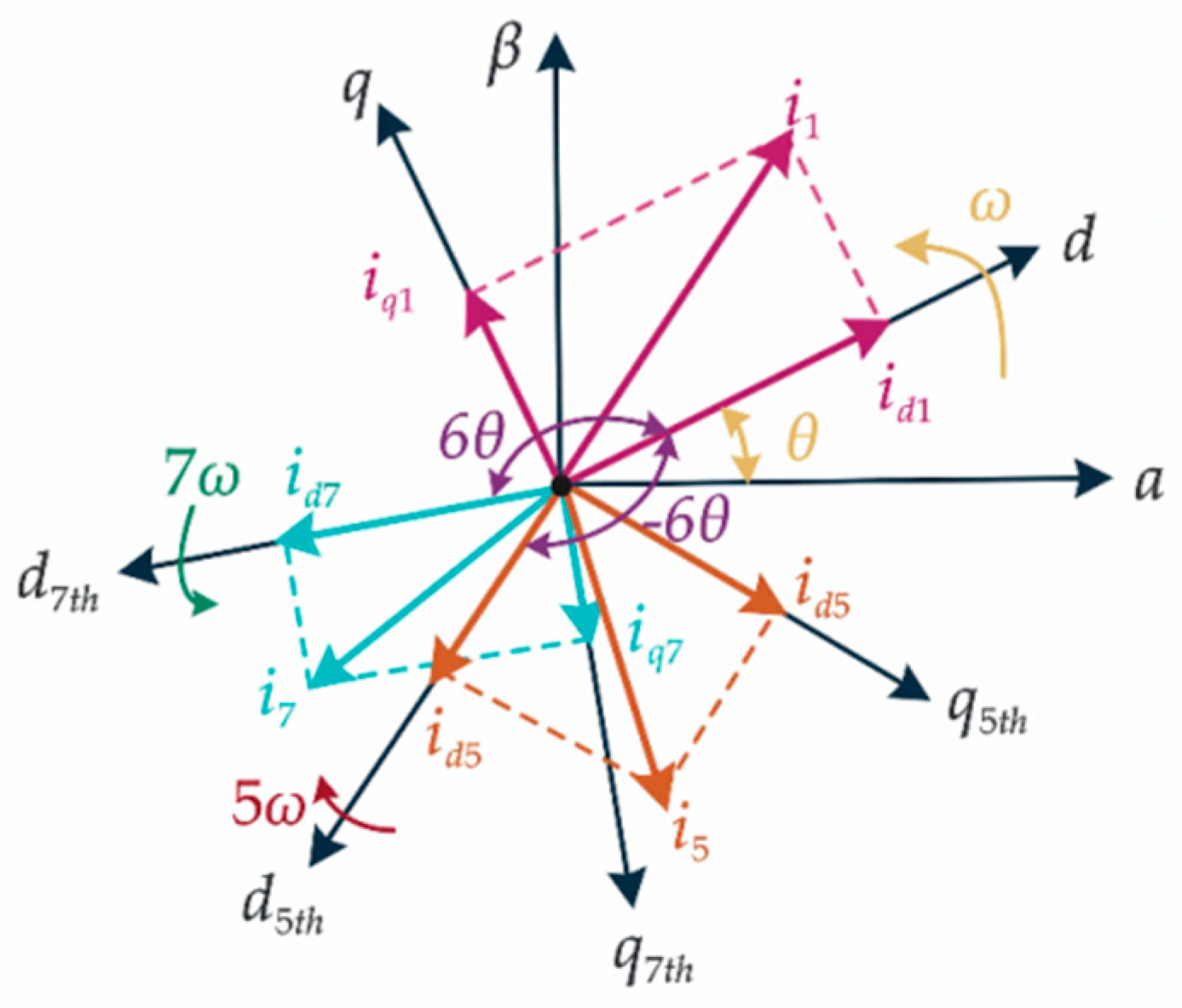
In the dq synchronous reference frame, the fundamental current appears as a DC component, whereas harmonic currents appear as AC components. Similarly, the harmonic components in the dq frame can be transformed into DC components in a synchronous reference frame rotating at the same frequency as the harmonic current. The multiple synchronous reference frames of the IPMSM are illustrated in Figure 9.
In Figure 9, the αβ coordinate system is the stationary reference frame; the dq frame rotates synchronously with the rotor at a speed of ω; the dq7th frame rotates in the same direction as the dq frame at 7ω; and the dq5th frame rotates in the opposite direction to the dq frame at 5ω. The transformation matrices between the dq frame and the harmonic frames are given as follows:
T d q d q 5 t h = cos ( 6 ω t ) sin ( 6 ω t ) sin ( 6 ω t ) cos ( 6 ω t )
T d q d q 7 t h = cos ( 6 ω t ) sin ( 6 ω t ) sin ( 6 ω t ) cos ( 6 ω t )
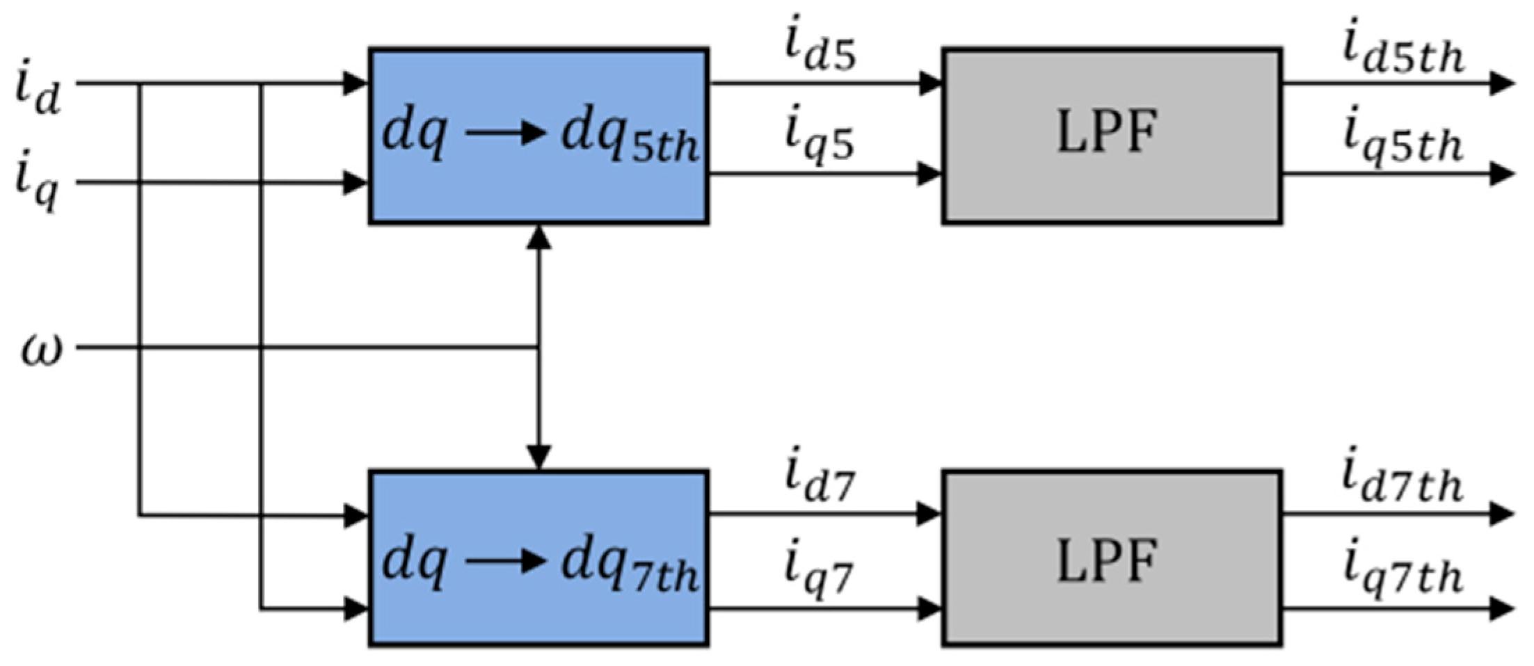
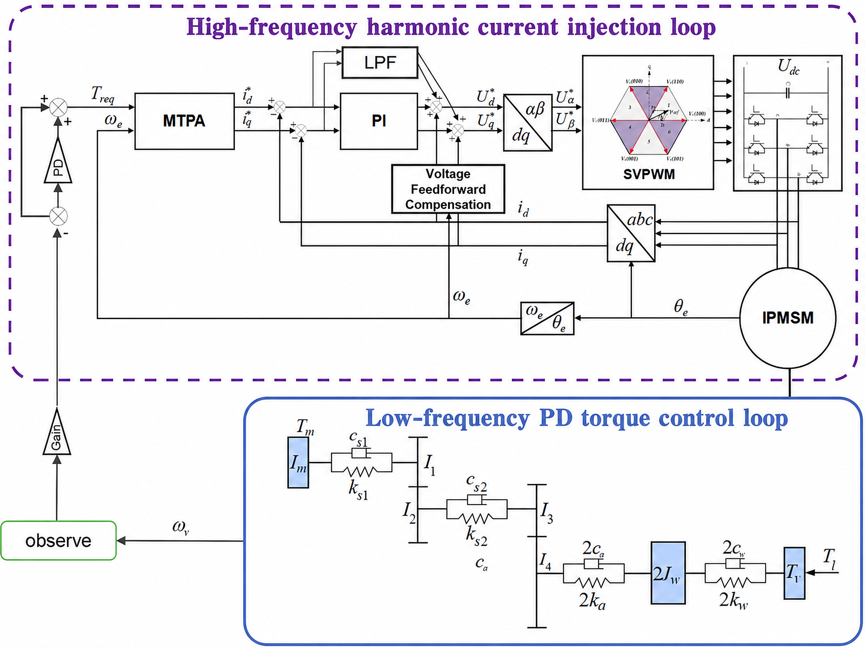
According to the above analysis, the harmonic current extraction model is shown in Figure 10. The fifth and seventh harmonic components in the three-phase current are extracted through coordinate transformation and a low-pass filter (LPF).
In Figure 10, id5th and iq5th represent the d-axis and q-axis components of the fifth harmonic current in the dq5th frame, respectively. id7th and iq7th represent the d-axis and q-axis components of the seventh harmonic current in the dq7th frame, respectively.
(2)
Calculation of Harmonic Compensation Voltage.
Due to the cogging effect of the IPMSM, high-order components will be introduced into the permanent magnet flux linkage. However, these components can be neglected owing to their small amplitude. Substituting Equation (4) into the steady-state voltage equation of the IPMSM, the voltage equation containing harmonic components in the dq reference frame can be obtained as:
u d = R s i d 1 ω L q i q 1 + 5 ω L q i 5 t h sin ( 6 ω t + θ 5 ) + R s i 5 t h cos ( 6 ω t + θ 5 ) 7 ω L q i 7 t h sin ( 6 ω t + θ 7 ) + R s i 7 t h cos ( 6 ω t + θ 7 ) + u q = R s i q 1 + ω L d i d 1 + ω ψ f 5 ω L d i 5 t h cos ( 6 ω t + θ 5 ) + R s i 5 t h sin ( 6 ω t + θ 5 ) + 7 ω L d i 7 t h cos ( 6 ω t + θ 7 ) + R s i 7 t h sin ( 6 ω t + θ 7 ) +
Equation (17) is transformed from the dq reference frame to the fifth harmonic reference frame. The voltage equation in the dq5th frame can be expressed as:
u d = R s i d 1 cos ( 6 ω t + θ 4 ) ω L q i q 1 sin ( 6 ω t + θ 4 ) + 5 ω L q i q 5 t h + R s i d 5 t h 7 ω L q i 7 t h sin ( 12 ω t + θ 6 ) + R s i 7 t h cos ( 12 ω t + θ 6 ) + u q = R s i q 1 sin ( 6 ω t + θ 4 ) + ω L d i d 1 cos ( 6 ω t + θ 4 ) + ω ψ f cos ( 6 φ 1 ) 5 ω L d i d 5 t h + R s i q 5 t h + 7 ω L d i 7 t h cos ( 12 ω t + θ 6 ) + R s i 7 t h sin ( 12 ω t + θ 6 ) +
where θ4, θ6, and φ1 are the initial phase angles of the fundamental current, the seventh harmonic current, and the permanent magnet flux linkage in the dq5th frame, respectively.
In the dq5th frame, the fundamental current and the seventh harmonic current appear as AC components, while the fifth harmonic current appears as a DC component. Neglecting the AC components, the steady-state harmonic voltage equation in the fifth harmonic reference frame is given by:
u d 5 = R s i d 5 t h + 5 ω L q i q 5 t h u q 5 = R s i q 5 t h 5 ω L d i d 5 t h
where ud5 and uq5 are the d-axis and q-axis components of the fifth harmonic voltage in the dq5th frame, respectively.
Similarly, Equation (19) is transformed from the dq reference frame to the seventh harmonic reference frame. Neglecting the AC components, the steady-state harmonic voltage equation in the seventh harmonic frame is given by:
u d 7 = R s i d 7 t h 7 ω L q i q 7 t h u q 7 = R s i q 7 t h + 7 ω L d i d 7 t h
where ud7 and uq7 are the d-axis and q-axis components of the seventh harmonic voltage in the dq7th frame, respectively.
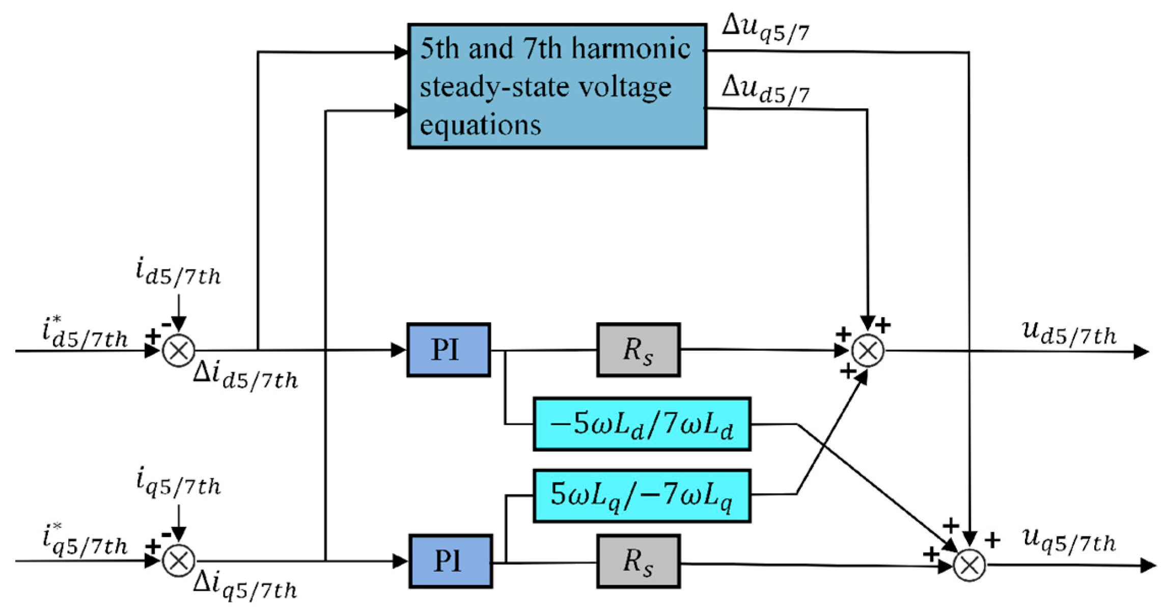
Based on the fifth and seventh steady-state harmonic voltage equations, a PI regulator with cross-product terms is designed to effectively counteract the influence of coupling components on the control. The schematic diagram for calculating the fifth and seventh harmonic compensation voltages is shown in Figure 11.

3.2. PD-Based Pole Placement Control

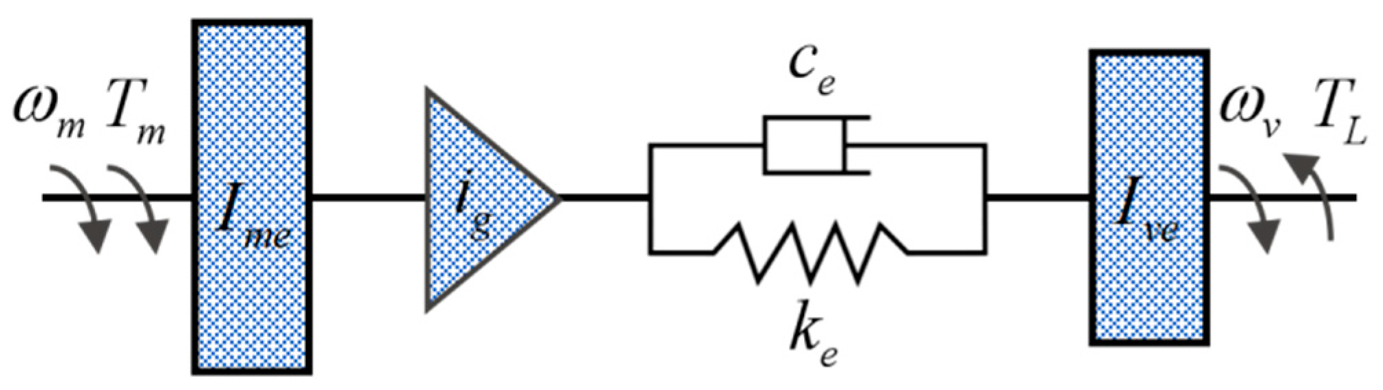
To facilitate the investigation of the influence of shaft flexibility on the drive system, the established electric drive system model needs to be simplified. The simplified model neglects the nonlinearities of the motor and gear backlash, yielding the regenerative braking system model shown in Figure 12.
The 7-DOF nonlinear model in Section 2 is retained as the mechanism analysis and validation model, whereas the following 2-DOF model is used only for small-signal controller synthesis around the nominal operating point. The reason for this reduction is that the PD pole placement controller targets the dominant low-frequency torsional mode between the motor-side equivalent inertia and the vehicle-side equivalent inertia. The high-frequency electromagnetic torque ripple is handled by HCI, while TVMS, mesh error and backlash are regarded as bounded perturbations in the low-frequency PD loop rather than state variables in the pole placement calculation. Therefore, the 2-DOF model does not replace the nonlinear 7-DOF model; it provides a tractable nominal plant for selecting closed-loop poles, and the robustness of the selected gains is subsequently checked using the nonlinear electromechanical coupling model.
The dynamic equations of the simplified system model are given by:
I m e ω ˙ m = T m - k e θ + c e ω m i g - ω v i g I v e ω ˙ v = k e θ + c e ω m i g - ω v - T L θ ˙ = ω m i g - ω v
The equivalent moments of inertia from the motor side to each stage of the reducer gears, and those from the tires to the entire vehicle side, are given by the following equations:
I m e = I m + I 1 + I 2 + I 3 i 1 2 + I 4 i g 2 I v e = 2 I w + I v
According to the principle of potential energy conservation, the equivalent stiffness and equivalent damping of the transmission system are given by the following equations:
k e = 2 k m o t k a k m i d k w i g 2 i 2 2 2 k m i d k a k w i 2 2 + 2 k m o t k a k w i g 2 + ( k a + k w ) k m o t k m i d i g 2 i 2 2 c e = 2 c m o t c a c m i d c w i g 2 i 2 2 2 c m i d c a c w i 2 2 + 2 c m o t c a c w i g 2 + ( c a + c w ) c m o t c m i d i g 2 i 2 2
According to Equations (22) and (23), the values of each equivalent parameter for the two-degree-of-freedom simplified model are listed in Table 5.
The simplification should be interpreted with the above scope. Under high-load/high-speed conditions, the neglected nonlinearities may increase the response amplitude and shift the exact resonance speed. Their influence can be summarized as follows: shaft stiffness mainly changes the equivalent natural frequency, damping changes the decay rate, load torque acts as an external disturbance, and backlash/TVMS introduce dead-zone and periodic excitation components. Consequently, the proposed PD-HCI method is suitable for broadband vibration suppression in the tested operating range, but the gains should be recalibrated when shaft stiffness, gear clearance or motor parameters deviate significantly from the prototype values.
For controller design, these uncertainties are considered bounded perturbations around the nominal equivalent plant. A local sensitivity interpretation was therefore added: decreasing the equivalent shaft stiffness moves the dominant torsional mode toward a lower frequency, reducing damping increases overshoot and settling time; load torque steps mainly excite the low-frequency torsional mode; and larger backlash increases impact-like oscillation around torque reversal. Under these perturbations, the PD controller mainly increases the damping of the dominant low-frequency mode, whereas the HCI loop attenuates the high-frequency electromagnetic torque ripple. This frequency band separation explains why the combined PD-HCI strategy can maintain suppression capability under moderate parameter deviations, although large deviations in stiffness, damping or backlash still require retuning of Kp, Kd and the feedforward gain.
Let the state variable be x = [ωm, ωv, θ]T. Then, the dynamic equation is given by:
x ˙ = c e I m e i g 2 c e I m e i g k e I m e i g c e I v e i g c e I v e k e I v e 1 i g 1 0 x + 1 I m e 0 0 u + 0 1 I v e 0 d y = 0 1 0 x
where u = Tm is the input variable, y = ωv is the output variable, and d = TL.
Furthermore, the parametric transfer function between wheel angular acceleration and motor torque can be derived as:
G m v _ T ( s ) = ω v ( s ) T m ( s )   =   b 1 s + b 0 s 3 + 2 ξ ω n s 2 + ω n 2 b 1 = c e I m e I v e i g b 0 = k e I m e I v e i g 2 ξ ω n = c e ( I m e i g 2 + I v e ) I m e I v e i g 2 ω n 2 = k e ( I m e i g 2 + I v e ) I m e I v e i g 2
G m a _ T ( s ) = ω ˙ v ( s ) T m ( s ) = ω a ( s ) T m ( s ) s = b 1 s + b 0 s 2 + 2 ξ ω n s + ω n 2
where b0 and b1 are the numerator coefficients of the transfer function and ξ and ωn represent the damping ratio and natural frequency of the system, respectively. Substituting the calculated parameters into the transfer function, the final expression is given as:
G m a _ T = 0.17 s + 185.96 s 2 + 3.35 s + 3628.46
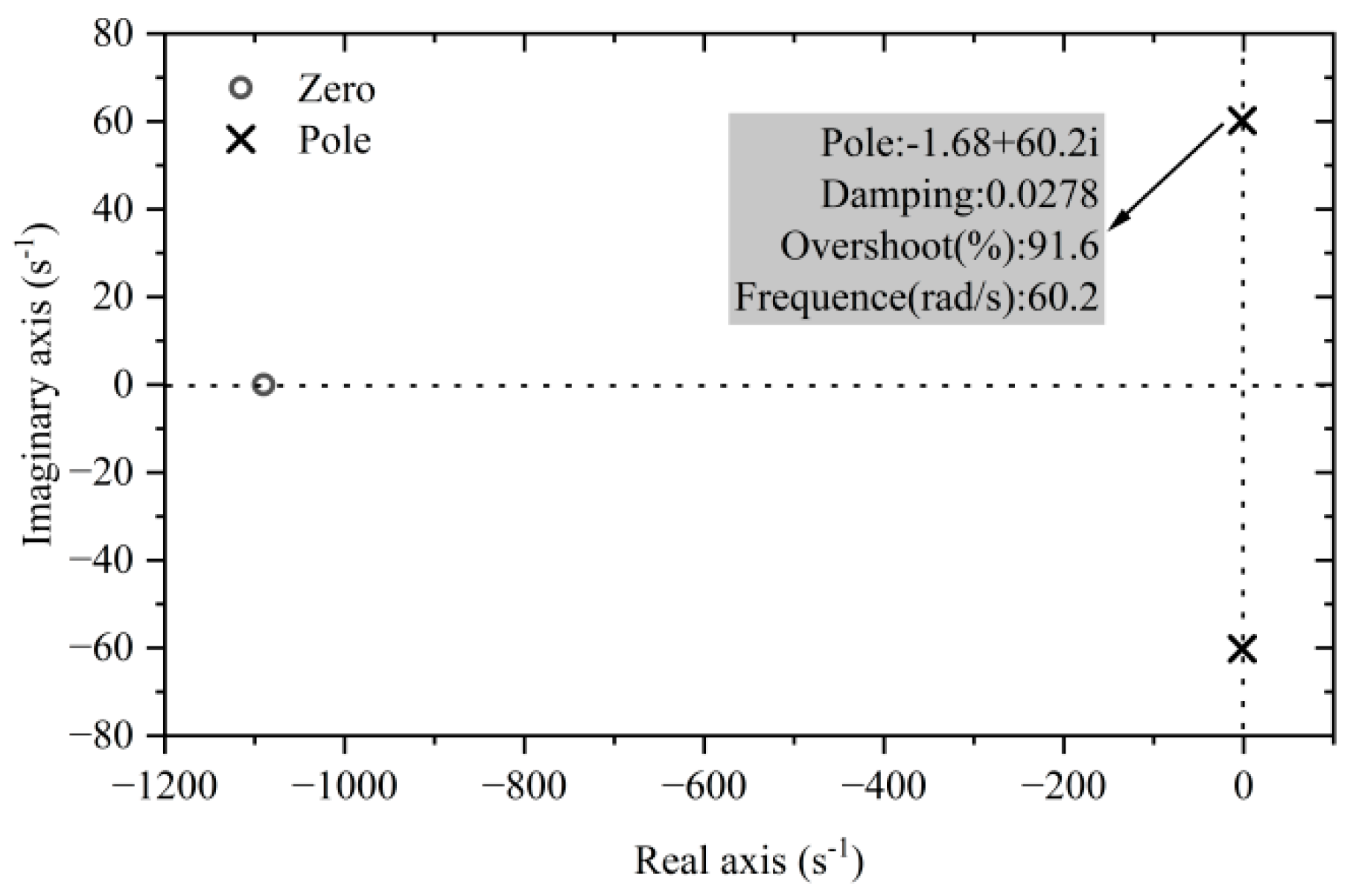
The pole–zero map is shown in Figure 13. A pair of complex conjugate poles of the system is located at −1.68 ± 60.2i, which lie very close to the imaginary axis, indicating an underdamped characteristic of the system. Through calculation, ξ = 0.0556 < 1 is obtained, which further verifies that the system is a typical underdamped system.
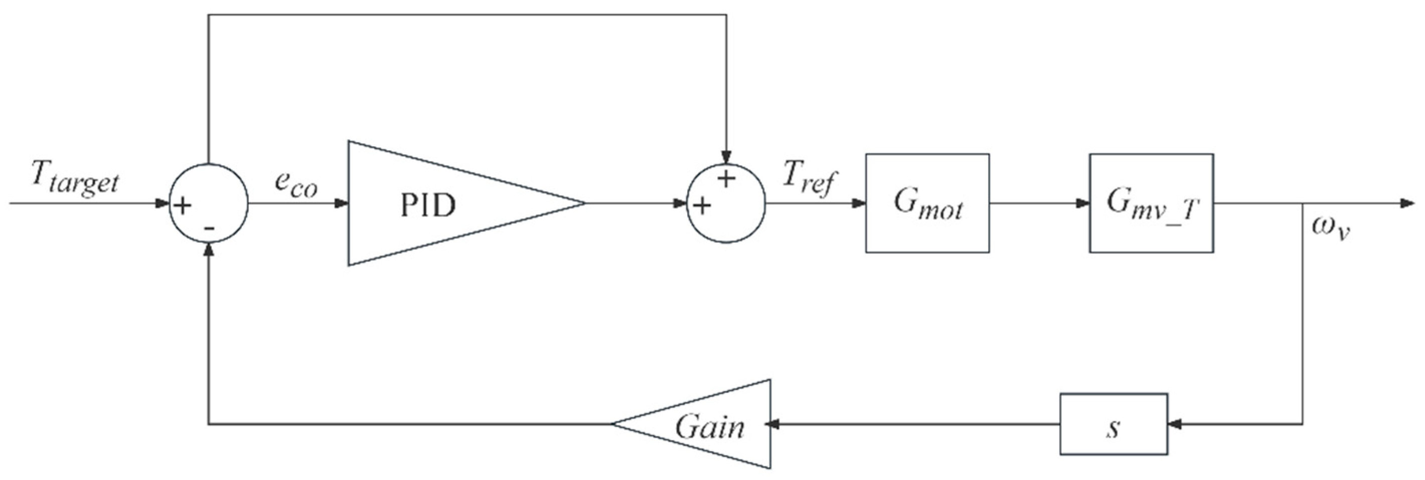
The controller structure is shown in Figure 14, which adopts a feedforward–feedback composite torque closed-loop control strategy. Taking the IPMSM as the core actuator, this strategy realizes the suppression of nonlinear characteristics of the drive system through angular acceleration calculation and PID dynamic regulation.
The transfer function of the motor is usually simplified as a first-order inertia element. To simplify the calculation process, assume Gmot(s) = 1. According to Figure 14, the following relationship can be obtained:
e c o   = T t a r g e t   G a i n s ω v T r e f   = G P I D   ( s ) e c o   + T t a r g e t ω v = G m v _ T   ( s ) T r e f  
The closed-loop transfer function of the system can be further derived as follows:
ω v ( s ) T t arg e t ( s ) = G m v _ T ( s ) G P I D ( s ) + 1 1 + G a i n s G m v _ T ( s ) G P I D ( s )
where Ttarget is the target motor torque, Tref is the motor control torque corrected by the controller, and the value of Tref is bounded by the maximum and minimum motor torque; eco denotes the error.
ω ˙ v ( s ) T t a r g e t ( s ) = a 2 s 2 + a 1 s + a 0 s 2 + 2 ξ ω n s + ω n 2 a 2 = 0.17 K d   ( 1 + 0.17 G a i n K d ) a 1 = ( 0.17 K p   + 0.17 + 185.97 K d   ) ( 1 + 0.17 G a i n K d ) a 0 = 185.97 ( K p   + 1 ) ( 1 + 0.17 G a i n K d ) 2 ξ ω n = ( 3.35 + 0.17 G a i n K p + 185.97 G a i n K d ) ( 1 + 0.17 G a i n K d ) ω n 2 = ( 3228.47 + 185.97 G a i n K p ) ( 1 + 0.17 G a i n K d )
The controller gains were not obtained by purely empirical trial and error. The tuning procedure was based on pole placement: the desired closed-loop characteristic polynomial was defined as Δd(s) = (s + 5.51)2 = s2 + 11.02s + 30.36 so that the dominant pair of poles became repeated real poles and the damping ratio approached ξ = 1. By substituting the PD controller into the closed-loop transfer function and equating the denominator coefficients with Δd(s), the nominal controller parameters Kp = 1.51 and Kd = 0.46 were obtained. The feedforward gain was then adjusted to Gain = 1.5 to compensate the torque command amplitude while keeping Tref within the motor torque limitation. Substituting the calculated parameters into the transfer function, the final expression is given as follows:
ω ˙ v T t a r g e t = 0.0695 s 2 + 76.43 s + 418.79 s 2 + 120.41 s + 3628.4
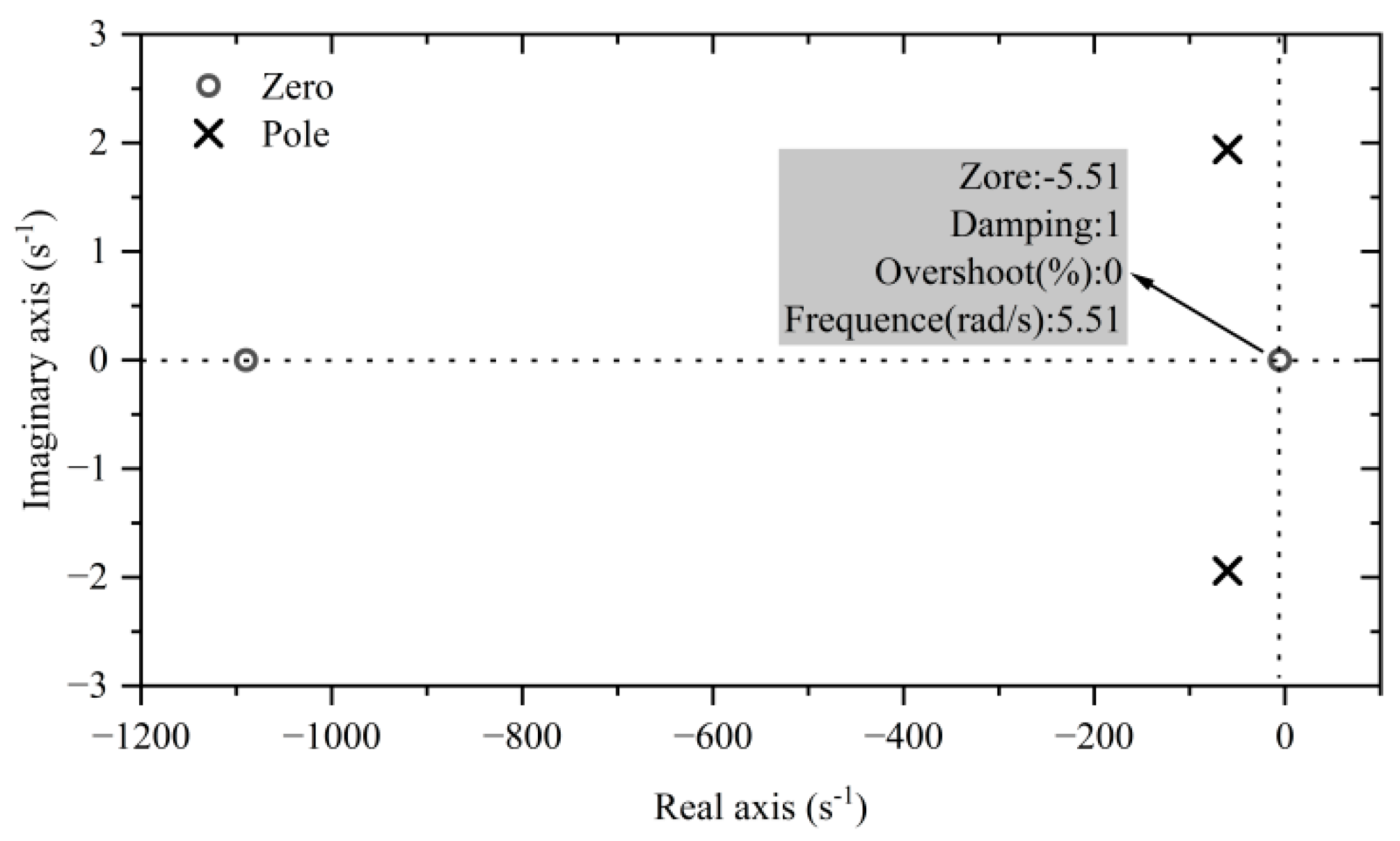
The pole–zero map is shown in Figure 15. The poles of the system are obtained as s1 = s2 = −5.51, which are two equal negative real roots, indicating that the system has reached a stable state. The calculated result ξ = 1 further verifies that the system is in a critically damped state.
Therefore, the schematic diagram of the torsional vibration suppression method based on PD-HCI is shown in Figure 16.
Compared with adaptive control, model predictive control, sliding-mode control, active disturbance rejection control and intelligent optimization-based methods, the PD-HCI scheme has a simpler structure and lower computational burden. It does not require online optimization, high-bandwidth disturbance observers or data-driven training; therefore, it is easier to implement on an electric-drive controller. Its limitation is that the PD part relies on nominal equivalent parameters, so large variations in stiffness, damping or backlash may require gain recalibration; this is why the original nonlinear model is retained for verification.
More specifically, adaptive control can improve robustness to parameter drift, but it requires reliable online parameter identification; model predictive control can explicitly handle constraints, but the online optimization burden is relatively high for a high-sampling-rate motor controller; sliding-mode control is robust to matched disturbances, but chattering may introduce additional torque ripple and NVH concerns; active disturbance rejection control can suppress unknown disturbances, but its performance depends on observer bandwidth and noise sensitivity; and intelligent optimization-based methods are effective for offline parameter tuning but are less suitable for deterministic real-time execution. Compared with these methods, the proposed PD-HCI method is less general for large uncertainty ranges, but it provides a practical compromise between vibration suppression, computational complexity and embedded implementability by separating low-frequency torsional damping from high-frequency harmonic compensation.

4. Simulation Analysis Based on the PD-HCI Method

4.1. Simulation Analysis

The dynamic performance of the torque-controlled IEDS is evaluated using the torque fluctuation rate, speed fluctuation rate, and total harmonic distortion (THD) of the current. The calculation formula for the torque fluctuation rate is given as follows:
T r i p = T max T min T r e f
where Tmax is the maximum torque, Tmin is the minimum torque, and Tref is the average torque.
The calculation formula for the speed fluctuation rate is given as follows:
n r i p = n max n min n r e f
where nmax is the maximum speed, nmin is the minimum speed, and nref is the average speed.
The calculation formula of THD is given as follows:
T H D = P 2 + P 3 + P 4 + P n P 1
where P1 is the amplitude of the fundamental component and Pn is the amplitude of the nth harmonic component.
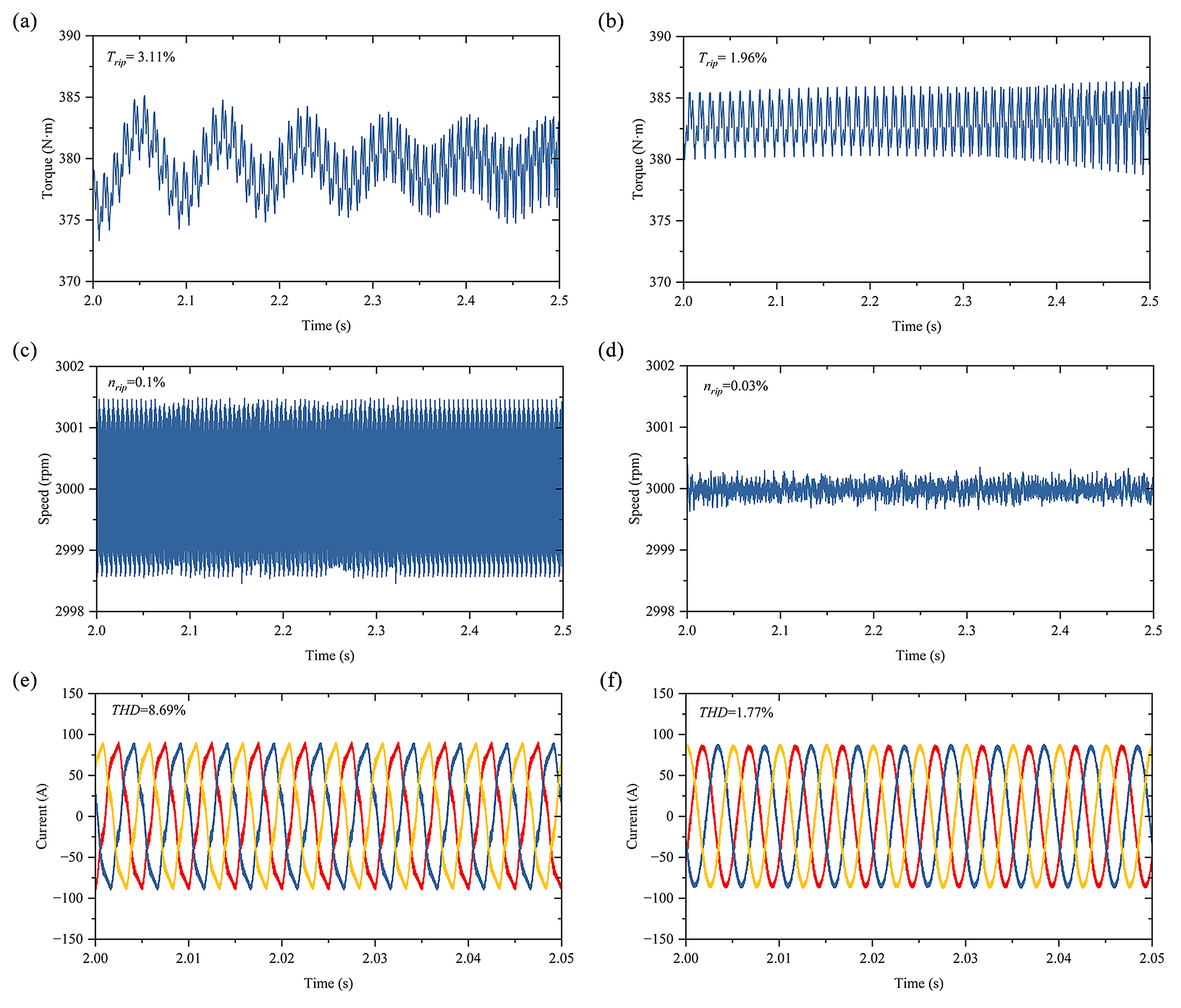
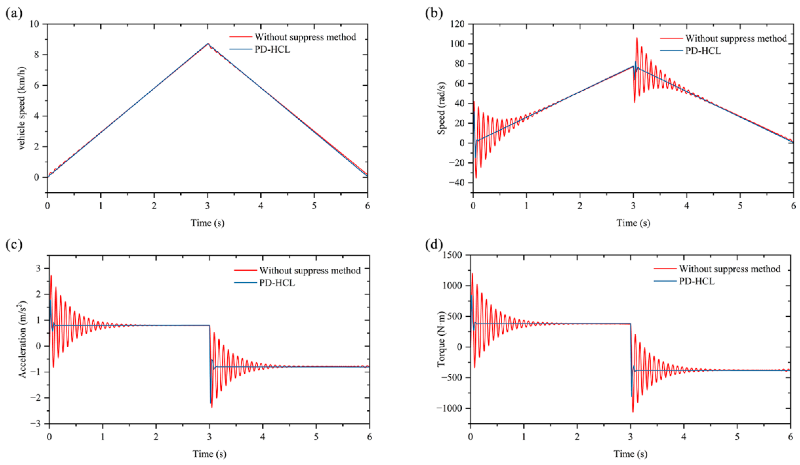
To verify the effectiveness of the proposed PD-harmonic compensation control strategy, an IEDS simulation model is established in the MATLAB R2022a environment, and transient condition tests are conducted. As shown in Figure 17, the motor first operates stably for 3 s under the working conditions of a reference speed of 3000 r/min and a load torque of 40 N·m; subsequently, a reverse load torque of −40 N·m is applied at the 3 s mark, and its transient response characteristics are presented in Figure 18.
Figure 17a,b show the half-shaft torque fluctuations from 2 s to 2.5 s under this operating condition. Without PD-HCI control, the system torque fluctuation is relatively significant, with a peak-to-peak value (T_pp) of 11.8002 N·m. The maximum and minimum torques are 385.1280 N·m and 373.3278 N·m, respectively; the average torque is 379.5594 N·m, and the calculated torque fluctuation rate is 3.11%. After introducing PD-HCI control, the torque ripple suppression effect is obvious. Although the average torque is slightly increased to 383.0341 N·m (an increase of about 0.9%), the torque peak-to-peak value is significantly reduced to 7.5239 N·m, a decrease of 36.2%. Correspondingly, the torque fluctuation rate is reduced from 3.11% to 1.96%, with a fluctuation suppression rate of approximately 37.0%. The low-frequency vibration generated by the transmission system is suppressed.
Figure 17c,d show the half-shaft speed fluctuations from 2 s to 2.5 s under this operating condition. Without PD-HCI control, the motor speed exhibits obvious periodic ripple. The maximum and minimum speeds are 3001.4959 rpm and 2998.4598 rpm, respectively; the average speed is stable near 3000 rpm (2999.9999 rpm), and the speed fluctuation rate is 0.10%. After adopting the PD-HCI control strategy, the speed smoothness is significantly improved. The speed peak-to-peak value is greatly reduced to 0.7523 rpm, with a decrease of 75.2%. Correspondingly, the speed fluctuation rate drops from 0.10% to 0.03%, and the suppression rate reaches 70.0%. Meanwhile, the average speed remains at 2999.9842 rpm, and the deviation from the target speed of 3000 rpm is negligible.
Figure 17e,f show the three-phase current waveforms from 2 s to 2.05 s under this operating condition. Taking ia as an example, the THD under this condition is analyzed. Without PD-HCI control, the stator current waveform is of poor quality, with a THD as high as 8.693%, among which the low-order harmonic components are particularly prominent. The fifth harmonic amplitude reaches 6.9523 A, accounting for 8.28% of the fundamental amplitude, which is the main harmonic source; the seventh harmonic amplitude is 1.4085 A, accounting for 1.68%. The two together contribute nearly 10% of the harmonic energy, which is the main cause of current ripple and torque ripple. After introducing the PD-HCI control strategy, the sinusoidal quality of the current waveform is significantly improved, and the THD is reduced to 1.772%. Notably, the fifth and seventh harmonics are completely suppressed in the ranking of main harmonic components. The high-frequency vibration generated by the motor is thus suppressed.
Figure 18a shows the vehicle speed response curve within 0–6 s. Under the two conditions of no harmonic suppression strategy (red curve) and the proposed PD-HCI control (blue curve), the vehicle speed curves almost completely coincide. The speed tracking trajectories during acceleration and deceleration are in good agreement; the peak vehicle speeds both reach approximately 8.7 km/h, and no obvious deviation is observed in the acceleration and deceleration slopes. The results indicate that the proposed PD-HCI control strategy can effectively suppress current harmonics and torque ripple without adversely affecting the dynamic response characteristics of the vehicle, and the system can still maintain satisfactory speed tracking accuracy and dynamic response performance.
Figure 18b shows the motor shaft response curve within 0–6 s. In the uniform acceleration phase from 0 to 3 s, without harmonic suppression (red curve), the motor speed exhibits obvious periodic sawtooth fluctuations, and the duration of speed fluctuation exceeds 1.5 s. In contrast, with PD-HCI control (blue curve), the speed trajectory is smooth and regular, the acceleration quickly converges to a steady-state value after startup, and the settling time of fluctuation is significantly shortened to within 0.25 s. The system achieves smooth speed tracking at the initial stage of acceleration. During the transient process of sudden load torque change at 3 s (stepping from 40 N·m to −40 N·m), the motor speed experiences severe overshoot and oscillation without control: the speed peak surges to approximately 110 rad/s and then drops rapidly to about 60 rad/s, corresponding to large positive and negative acceleration shocks (maximum and minimum acceleration), with slow oscillation decay and a long settling time of about 1.5 s. The PD-HCI control strategy effectively suppresses speed overshoot, limits the speed fluctuation amplitude within 10 rad/s, shortens the settling time to within 0.25 s, and significantly reduces the absolute values of maximum/minimum acceleration during acceleration and deceleration.
Figure 18c shows the dynamic response curve of vehicle longitudinal acceleration within 0–6 s. In the uniform acceleration phase from 0 to 3 s, without harmonic suppression (red curve), the acceleration shows obvious high-frequency oscillation: the maximum acceleration peak reaches approximately 2.2 m/s2, the minimum acceleration valley is about −0.5 m/s2, the acceleration fluctuation range exceeds 2.7 m/s2, and the oscillation gradually converges after lasting until about 1.5 s. In contrast, with PD-HCI control (blue curve), the acceleration quickly stabilizes near 0.8 m/s2 after startup, the maximum and minimum acceleration fluctuation range is controlled within 1.2 m/s2, and the transient overshoot is significantly reduced. During the transient process of sudden load torque change at 3 s (stepping from 40 N·m to −40 N·m), the vehicle suffers severe deceleration shock without control. The minimum acceleration drops sharply to about −2.8 m/s2, followed by a strong positive acceleration rebound with the maximum acceleration reaching approximately 0.5 m/s2, seriously deteriorating the subjective riding comfort of passengers. The PD-HCI control strategy effectively suppresses the shock amplitude: the minimum acceleration is only about −2.3 m/s2 and the maximum acceleration is about 0.5 m/s2, with a narrower acceleration fluctuation range and fast oscillation decay. The proposed harmonic compensation method significantly suppresses the extreme acceleration fluctuations during acceleration and deceleration, effectively reduces the maximum positive acceleration shock and maximum negative acceleration (deceleration) shock caused by torque mutation, and greatly improves the ride smoothness and comfort of the vehicle.
Figure 18d shows the dynamic response curve of half-shaft torque within 0–6 s. In the acceleration phase from 0 to 3 s, without harmonic suppression (red curve), the half-shaft torque exhibits severe periodic fluctuations. The maximum torque peak reaches approximately 1200 N·m, the minimum torque valley is about −300 N·m, the peak-to-peak fluctuation exceeds 1500 N·m, and the oscillation lasts for a long time, indicating significant torsional vibration in the drive system. In contrast, with PD-HCI control (blue curve), the half-shaft torque converges rapidly to the steady-state value, the maximum torque overshoot is controlled within 400 N·m, the torque fluctuation amplitude is significantly reduced, and the transmission smoothness is remarkably improved. During the transient process of sudden load torque change at 3 s (switching from driving to braking), the half-shaft torque produces extreme impact and overshoot without control. The maximum torque peak is about 250 N·m, while the minimum torque drops sharply to approximately −1200 N·m. The PD-HCI control strategy effectively suppresses the torque extremes: the maximum torque is reduced to about 200 N·m, and the minimum torque to approximately −750 N·m, with fast oscillation decay, and the system returns to steady state within 0.25 s. The proposed PD-HCI harmonic compensation method significantly suppresses the extreme fluctuations in half-shaft torque during steady-state operation and load sudden change, effectively reducing the maximum impact torque and torsional vibration amplitude of the transmission system.
These transient results also support the validity of the pure torsional model for the present research objective. The large uncontrolled oscillations in motor speed, acceleration and half-shaft torque correspond to the dominant torsional resonance identified by the Campbell analysis, while the controlled responses show increased damping of the low-frequency torsional mode and reduced high-frequency harmonic excitation. Thus, although the model does not include non-torsional structural modes, it captures the actual dynamic behavior that is most relevant to shaft torque transmission and resonance-induced NVH degradation in the tested IEDS.

4.2. Experimental Verification

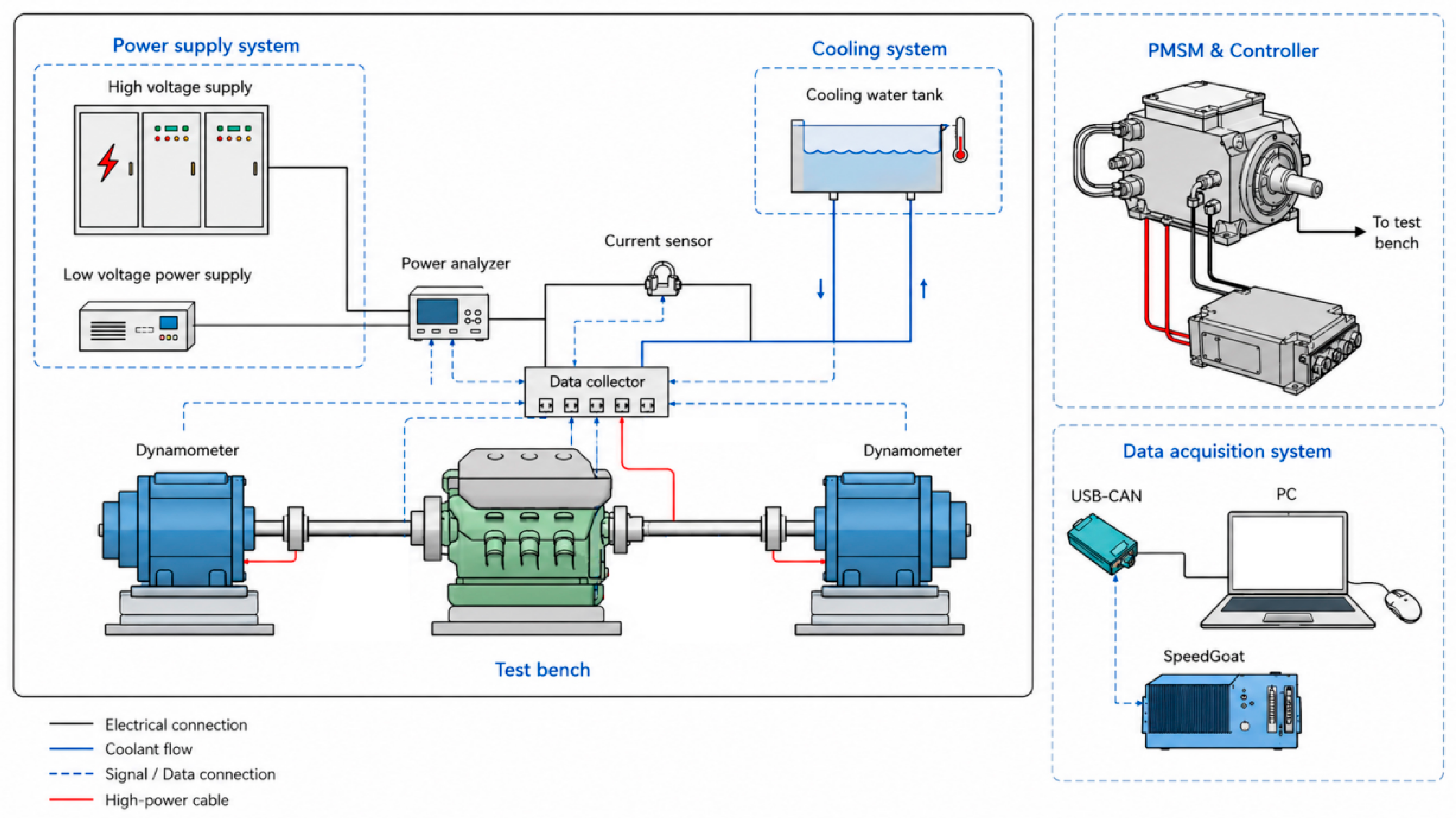
As shown in Figure 19, the experimental platform is a comprehensive system designed for motor performance testing and control validation. The tested IPMSM serves as the core of the system, and it is connected to dynamometers on both sides via couplings to complete loading and energy feedback. The motor is supplied by a high-voltage power supply, whereas the low-voltage power supply delivers stable electric power for the control and measurement units. During the experiment, the real-time operating conditions of the motor are captured by current sensors. These sensing signals, along with voltage, current and power parameters collected by the power analyzer, are transmitted to the data collector for multi-channel synchronous recording. An independent cooling water tank is configured to guarantee the thermal stability of key components under long-duration operation, which realizes temperature regulation through circulating cooling. For control and communication, a USB-CAN interface is utilized for data transmission between the host computer and the motor controller. Cooperating with the Speedgoat real-time simulation platform, the upper PC completes rapid deployment and online debugging of control algorithms.
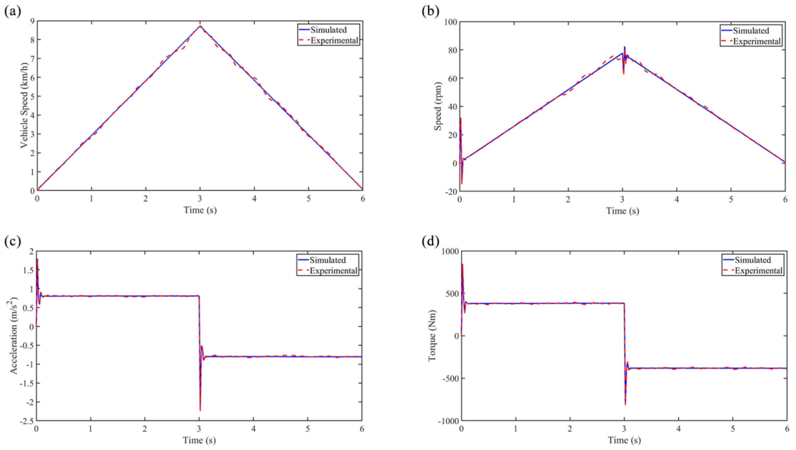
The test was conducted under the same speed and load settings as the simulation. The dynamometer provided programmable load torque, while the Speedgoat platform executed the control algorithm in real time and exchanged command/feedback signals with the motor controller through the CAN interface. Before comparison, the experimental and simulation signals were time-aligned according to the start of the speed command, and the steady-state offset of the torque sensor was removed. Each operating condition was recorded over repeated runs, and the representative curves in Figure 20 correspond to the data set with the most complete synchronized signals.
Figure 20 presents a comparison between the simulation results and experimental data on rotational speed, torque, acceleration and vehicle speed under typical operating conditions. The error analysis shows that the mean absolute error (MAE) and root mean square error (RMSE) of vehicle speed are 0.0574 and 0.0791, respectively, with a maximum error of 0.2804 and a coefficient of determination (R2) of 0.9990. For rotational speed, the MAE is 0.6197, the RMSE is 0.9410, the maximum error is 2.8391, and the R2 is 0.9982. The acceleration achieves an MAE of only 0.0120, an RMSE of 0.0147, a maximum error of 0.0484, and a high R2 of 0.9997. In terms of torque, the MAE and RMSE are 4.9560 and 6.2570, with a maximum error of 15.8336. Although its absolute error is relatively large, the R2 still reaches 0.9997. Comprehensive analysis indicates that the coefficients of determination of all variables are close to 1, demonstrating a high consistency between simulation results and experimental data. Among all indicators, acceleration and vehicle speed show the minimum error, which proves that the established model possesses high accuracy in dynamic response and overall output prediction. There exists a certain deviation in rotational speed during the transient stage, while the overall changing trend remains consistent. The relatively larger torque error is mainly attributed to abrupt load changes and unmodeled dynamics in the experimental bench. Possible sources include the finite response delay of the dynamometer and motor controller, coupling compliance, temperature-dependent resistance and magnetic saturation, sensor noise and time-synchronization error among the data acquisition channels. These factors have a more direct influence on torque than on speed or acceleration, especially during transient load reversal. Therefore, the torque error does not invalidate the overall trend agreement. Overall, the proposed model can accurately reflect the dynamic and steady-state characteristics of the system, thus possessing favorable engineering application value.

5. Conclusions

This paper focuses on the NVH performance degradation caused by broadband torsional vibration in the IEDS of electric vehicles and conducts an investigation on the electromechanical coupling torsional vibration mechanism and cooperative active control. Firstly, a refined electromechanical coupling dynamic model is established, which considers the electromagnetic nonlinearity of the motor and the gear transmission nonlinearity. The inherent characteristics and critical speed range of the system are clarified, and the generation mechanism and high–low frequency coupling characteristics of full-band torsional vibration in the IEDS are revealed. On this basis, a cooperative active control strategy based on PD pole placement and harmonic current injection (PD-HCI) is proposed, which realizes the cooperative suppression of low-frequency transmission torsional vibration and high-frequency electromagnetic ripple through frequency band division. Simulation results show that the proposed strategy can reduce the steady-state torque fluctuation rate from 3.11% to 1.96%, the speed fluctuation rate from 0.10% to 0.03%, and the THD of stator current from 8.69% to 1.77%. Meanwhile, it significantly improves the system stability under transient load shock conditions without obvious degradation of dynamic performance. Experimental results indicate that, despite certain errors under partial transient operating conditions, the overall deviations are within an acceptable range. The simulation results accurately reflect the dynamic and steady-state characteristics of the system, which verifies the effectiveness and reliability of the established model. The research outcomes of this study enrich the analytical theory of electromechanical coupling torsional vibration for integrated electric drive systems. The proposed control method requires no hardware modification and is convenient for engineering implementation. It can provide theoretical support and technical references for the NVH performance optimization of electric vehicle electric drive systems.
Nevertheless, the present study still has limitations. The experimental verification is performed on a bench platform under typical operating conditions, and the pure torsional model does not include bearing flexibility, housing vibration, axial/lateral gear dynamics or temperature-dependent magnetic saturation. For vehicle-level application, further HIL and road test verification under broader high-speed, high-load and resonance-near conditions will be required, together with formal uncertainty quantification of shaft stiffness, damping, backlash and load torque. These issues will be addressed in future work.
In future work, the present qualitative uncertainty discussion will be extended to a formal uncertainty quantification framework, such as multi-parameter sensitivity analysis or Monte Carlo simulation, to evaluate the combined influence of shaft stiffness, damping, load torque and backlash on resonance speed, torque ripple and controller margin. Additional comparisons with adaptive control, MPC, sliding-mode control and ADRC under the same computational constraints will also be conducted to further define the practical application boundary of the proposed PD-HCI strategy.

Author Contributions

Conceptualization, Y.M.; software, Y.M., Z.H., D.H., J.Y. and H.H.; formal analysis, Y.M., H.H., D.H., J.Y. and Z.H.; investigation, Y.M., Z.H., D.H., H.H., J.Y., K.C., J.H. and F.J.; resources, Y.M.; writing—original draft preparation, Y.M., Z.H. and H.H.; writing—review and editing, Y.M., Z.H., D.H., H.H., J.Y., K.C., J.H. and F.J.; supervision, Y.M.; funding acquisition, Y.M., H.H., K.C. and J.H. All authors have read and agreed to the published version of the manuscript.

Funding

This work was supported by the Guangxi Key Research and Development Program Project, GuiKeAB25069449, the “Jianfeng” Action Plan (Guangxi Key Special Project Program), GuiKeJF2503980004, and the Guangxi National Science and Technology Major Project: GuiKeAA24206064.

Data Availability Statement

All data used to support the findings of this study are included within this article.

Conflicts of Interest

The authors declare no conflicts of interest regarding the publication of this paper.

Nomenclature

ωeThe electrical angular velocity
RsThe stator resistance
ψdThe d-axis flux linkage
ψqThe q-axis flux linkage
i1The amplitudes of the fundamental current
i5thThe amplitudes of the fifth harmonic current
i7thThe amplitudes of the seventh harmonic current
θ1The initial phase angles of the fundamental current
θ2The initial phase angles of the fifth harmonic current
θ3The initial phase angles of the seventh harmonic current
id1The d-axis component of the fundamental current
iq1The q-axis component of the fundamental current
θ5The initial phase angles of the fifth harmonic current
θ7The initial phase angles of the seventh harmonic current
PnThe number of pole pairs
ImThe moment of inertia
BThe viscous damping coefficient
TLThe load torque
ωmThe mechanical angular velocity of the motor
TmThe electromagnetic torque
TlThe driving resistance torque of the vehicle
IpThe moment of inertia of the driving gear
RgThe base circle radius of the driven gear
θpThe rotation angles of the driving gear
cgThe meshing damping
kgThe time-varying meshing stiffness
e(θp)The meshing error
xThe relative displacement
emThe average meshing error
e0The amplitude of the total tangential composite deviation
bThe half of the gear backlash
id5thThe d-axis component of the fifth harmonic current in the dq5th frame
φ1The initial phase angles of the permanent magnet flux linkage in the dq5th frame
ud5The d-axis component of the fifth harmonic voltage in the dq5th frame
ξThe damping ratio
ωnThe natural frequency
TtargetThe target motor torque
TrefThe motor control torque corrected by the controller
TmaxThe maximum torque
nrefThe average speed
P1The amplitude of the fundamental component

References

  1. Zhang, W.; Fang, X.; Sun, C. The alternative path for fossil oil: Electric vehicles or hydrogen fuel cell vehicles? J. Environ. Manag. 2023, 341, 118019. [Google Scholar] [CrossRef]
  2. Sun, Z.; Hu, J.; Yao, Z.; Xue, S. Optimization of electromagnetic vibration for integrated electric drive systems based on electric vehicle driving cycle considering energy consumption. Energy 2024, 313, 134018. [Google Scholar] [CrossRef]
  3. Zhang, B.; Song, Z.; Liu, S.; Huang, R.; Liu, C. Overview of Integrated Electric Motor Drives: Opportunities and Challenges. Energies 2022, 15, 8299. [Google Scholar] [CrossRef]
  4. Wang, S.; Zhang, H.; Li, J.; Zhao, P.; Xu, X.; Dong, P. Review on the Development Trends of Electric Drive Systems for Electric Vehicles. In Proceedings of the 2024 IEEE 22nd International Conference on Industrial Informatics (INDIN), Beijing, China, 18–20 August 2024; pp. 1–6. [Google Scholar] [CrossRef]
  5. Hazra, S.; Khan, A. A Review on Electric Vehicle NVH Challenges and Recent Trends; SAE Technical Paper 2025-01-0042; SAE International: Warrendale, PA, USA, 2025. [Google Scholar] [CrossRef]
  6. Kurian, A.G.; Thakur, S.K.; Kunde, S.; Sankpal, K.; Wagh, S. Challenges in Electric Vehicle NVH. In Proceedings of the 2021 IEEE Transportation Electrification Conference (ITEC-India), New Delhi, India, 16–19 December 2021; pp. 1–6. [Google Scholar] [CrossRef]
  7. Horváth, K.; Zelei, A. Simulating Noise, Vibration, and Harshness Advances in Electric Vehicle Powertrains: Strategies and Challenges. World Electr. Veh. J. 2024, 15, 367. [Google Scholar] [CrossRef]
  8. Jia, H.; Hu, G.; Xu, X.; Liang, D.; Liu, C. Torsional Vibration Suppression in Multi-Condition Electric Propulsion Systems Through Harmonic Current Modulation. Actuators 2025, 14, 283. [Google Scholar] [CrossRef]
  9. Hu, J.; Guo, Q.; Sun, Z.; Yang, D. Study on low-frequency torsional vibration suppression of integrated electric drive system considering nonlinear factors. Energy 2023, 284, 129251. [Google Scholar] [CrossRef]
  10. Cui, Y.; Lu, H.; Xu, J.; Zhang, Y.; Zou, L. Study on Vibration Characteristics and Harmonic Suppression of an Integrated Electric Drive System Considering the Electromechanical Coupling Effect. Actuators 2025, 14, 386. [Google Scholar] [CrossRef]
  11. Sun, Z.; Hu, J.; Guo, Q. Torsional vibration analysis and suppression for integrated electric drive system considering nonlinear excitations. Commun. Nonlinear Sci. Numer. Simul. 2025, 145, 108695. [Google Scholar] [CrossRef]
  12. Fang, Z.; Li, Q.; Yao, L.; Hu, X. Stiffness Optimization for Hybrid Electric Vehicle Powertrain Mounting System in the Context of NSGA II for Vibration Decoupling and Dynamic Reaction Minimization. World Electr. Veh. J. 2025, 16, 131. [Google Scholar] [CrossRef]
  13. Abduh, S.; Karunanithi, S.; Nur, T. Analysis of the Cogging Torque Reduction in Permanent Magnet Generators for a Very Low Wind Speed. Energies 2025, 18, 2802. [Google Scholar] [CrossRef]
  14. Ocak, O.; Aydin, M. An Innovative Semi-FEA Based, Variable Magnet-Step-Skew to Minimize Cogging Torque and Torque Pulsations in Permanent Magnet Synchronous Motors. IEEE Access 2020, 8, 210775–210783. [Google Scholar] [CrossRef]
  15. Katona, M.; Orosz, T. Cogging Torque Reduction of a Flux-Intensifying Permanent Magnet-Assisted Synchronous Reluctance Machine with Surface-Inset Magnet Displacement. Energies 2025, 18, 5492. [Google Scholar] [CrossRef]
  16. Pranjić, F.; Virtič, P. Cogging Torque Reduction Techniques in Axial Flux Permanent Magnet Machines: A Review. Energies 2024, 17, 1089. [Google Scholar] [CrossRef]
  17. Shi, Z.; Sun, X.; Cai, Y.; Yang, Z.; Lei, G.; Guo, Y.; Zhu, J. Torque Analysis and Dynamic Performance Improvement of a PMSM for EVs by Skew Angle Optimization. IEEE Trans. Appl. Supercond. 2019, 29, 1–5. [Google Scholar] [CrossRef]
  18. Pleguezuelos, M.; Sánchez, M.B.; Pedrero, J.I. Analytical model for meshing stiffness, load sharing, and transmission error for spur gears with profile modification under non-nominal load conditions. Appl. Math. Model. 2021, 97, 344–365. [Google Scholar] [CrossRef]
  19. Hou, Y.; Liu, Z.; He, X.; Wang, S.; Liu, Q.; Zhou, X. Gearbox noise and vibration control based on multiple-objective optimization of helical gear microgeometry. Appl. Acoust. 2025, 240, 110955. [Google Scholar] [CrossRef]
  20. Liao, F.; Huang, J.; Zhu, W. Investigation on nonlinear vibration of a gear transmission system considering time-varying mesh stiffness and time-varying supporting stiffness. J. Sound. Vib. 2025, 603, 118957. [Google Scholar] [CrossRef]
  21. Andary, F.; Heinzel, C.; Wischmann, S.; Berroth, J.; Jacobs, G. Calculation of tooth pair stiffness by finite element analysis for the multibody simulation of flexible gear pairs with helical teeth and flank modifications. Multibody Syst. Dyn. 2023, 59, 395–428. [Google Scholar] [CrossRef]
  22. Chen, S.; Hu, M. Active torsional vibration suppression of integrated electric drive system based on optimal harmonic current instruction analytic calculation method. Mech. Mach. Theory 2023, 180, 105136. [Google Scholar] [CrossRef]
  23. Zhang, W.; Liang, X.; Han, Z.; Bu, L.; Liu, J.; Fu, B.; Jiang, M. Active Torsional Vibration Suppression Strategy for Power-Split-HEV Driveline System Based on Dual-Loop Control. Machines 2025, 13, 418. [Google Scholar] [CrossRef]
  24. Qu, J.; Jatskevich, J.; Zhang, C.; Zhang, S. Torque ripple reduction method for permanent magnet synchronous machine drives with novel harmonic current control. IEEE Trans. Energy Convers. 2021, 36, 2502–2513. [Google Scholar] [CrossRef]
  25. Yi, P.; Zheng, W.; Li, X. Overview of torque ripple minimization methods for permanent magnet synchronous motors based on harmonic injection. Chin. J. Electr. Eng. 2024, 10, 16–29. [Google Scholar] [CrossRef]
  26. Lyu, Z.; Wu, L.; Song, P. A novel harmonic current control method for torque ripple reduction of SPMSM considering DC-link voltage limit. IEEE Trans. Power Electron. 2023, 39, 2558–2568. [Google Scholar] [CrossRef]
  27. Dai, L.; Niu, S.; Yuan, X.; Chan, C.C. Data-Driven Current Harmonic Optimization for Minimizing Torque Ripple and Injection Losses in PMSM Drives. IEEE Trans. Ind. Electron. 2026, 73, 4495–4505. [Google Scholar] [CrossRef]
  28. Xu, J.; Yang, X.; Li, W.; Zheng, J.; Wang, Y.; Fan, M.; Zhou, W.; Lu, Y. Design of quasi-zero stiffness joint actuator and research on vibration isolation performance. J. Sound. Vib. 2020, 479, 115367. [Google Scholar] [CrossRef]
  29. Sun, K.; Tang, J.; Yang, Y.; Jiang, B.; Li, Y.; Cao, D. Active control of quasi-zero-stiffness vibration isolator with variable load. Int. J. Struct. Stab. Dyn. 2024, 24, 2450243. [Google Scholar] [CrossRef]
  30. Chen, L.; Xu, X.; Liang, C.; Jiang, X.-W.; Wang, F. Semi-active control of a new quasi-zero stiffness air suspension for commercial vehicles based on H2H state feedback. J. Vib. Control 2023, 29, 1910–1926. [Google Scholar] [CrossRef]
  31. Tuo, J.; Zheng, S.; Chen, X.; Wang, B.; Qi, W. Design of a quasi-zero stiffness vibration isolation and energy harvesting integrated seat suspension. J. Vib. Eng. Technol. 2025, 13, 222. [Google Scholar] [CrossRef]
  32. Sun, Z.; Hu, J.; Xin, Y.; Guo, Q.; Yao, Z.; Yang, Y. Active torsional vibration suppression for integrated electric drive system considering nonlinear factors. Nonlinear Dyn. 2024, 112, 17107–17127. [Google Scholar] [CrossRef]
  33. Yue, H.; He, H.; Han, M. Study on torsional vibration characteristics and suppression of electric vehicles with dual-motor drive system. J. Frankl. Inst. 2023, 360, 380–402. [Google Scholar] [CrossRef]
  34. Jiang, S.; Liu, S.; Wu, B.; Li, W. Active Suppression of Low-Speed Vibration in Electric Vehicle Drivelines Considering PMSM Torque Ripple. IEEE Trans. Energy Convers. 2026, 41, 248–261. [Google Scholar] [CrossRef]
  35. Cai, G.; Yin, G.; Pi, D.; Zhuang, W.; Feng, J.; Ren, Y.; Ding, H. Safety Region-Based Event-Driven Lateral Stability Control for DDEVs with Energy Conservation. IEEE Trans. Transp. Electrif. 2025, 11, 13976–13989. [Google Scholar] [CrossRef]
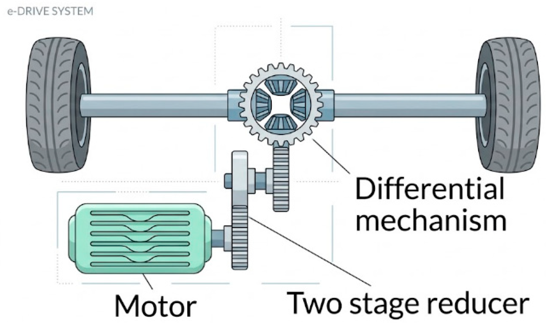
Figure 1. Structure of the IEDS.
Processes 14 01929 g001
Figure 2. Pure torsional dynamic model of the powertrain system.
Processes 14 01929 g002
Figure 3. Torsional dynamic model of gear pair meshing.
Processes 14 01929 g003
Figure 4. Time-varying stiffness curve.
Processes 14 01929 g004
Figure 5. Campbell diagram.
Processes 14 01929 g005
Figure 6. Influence of time-varying mesh stiffness on the transmission system. (a) Motor shaft speed; (b) half-shaft torque.
Processes 14 01929 g006
Figure 7. Influence of mesh error on the transmission system. (a) Motor shaft speed; (b) half-shaft torque.
Processes 14 01929 g007
Figure 8. Influence of gear backlash on the transmission system. (a) Motor shaft speed; (b) half-shaft torque.
Processes 14 01929 g008
Figure 9. The multiple synchronous reference frames of the IPMSM.
Processes 14 01929 g009
Figure 10. Harmonic current extraction model.
Processes 14 01929 g010
Figure 11. Block diagram of harmonic compensation voltage calculation.
Processes 14 01929 g011
Figure 12. Simplified model of the drive system.
Processes 14 01929 g012
Figure 13. Pole–zero map.
Processes 14 01929 g013
Figure 14. Simplified model of the regenerative braking system.
Processes 14 01929 g014
Figure 15. Pole–zero map.
Processes 14 01929 g015
Figure 16. Schematic diagram of torsional vibration suppression method based on PD-HCI.
Processes 14 01929 g016
Figure 17. Comparison of system responses between unsuppressed control and PD-HCI control Under steady-state conditions. (a) Half-shaft torque: without suppression method; (b) half-shaft torque: PD-HCI; (c) motor speed: without suppression method; (d) motor speed: PD-HCI; (e) current: without suppression method; (f) current: PD-HCI.
Processes 14 01929 g017
Figure 18. Comparison of system dynamic responses between unsuppressed control and PD-HCI control under transient conditions. (a) Vehicle speed; (b) motor shaft speed; (c) vehicle acceleration; (d) half-shaft torque.
Processes 14 01929 g018
Figure 19. Schematic diagram of the experimental setup.
Processes 14 01929 g019
Figure 20. Comparison diagram of simulation results and experimental data. (a) Vehicle speed; (b) motor shaft speed; (c) vehicle acceleration; (d) half-shaft torque.
Processes 14 01929 g020
Table 1. Basic parameters of the IPMSM.
ParameterValue
Ld0.9 mH
Lq1.8 mH
ψf0.150 Wb
Pn4
Rs0.035 Ω
Maximum motor power180 N·m
Rated voltage350 V
Table 2. Main parameters of the vehicle and transmission system.
Parameter SymbolDefinitionValue
ImEquivalent moment of inertia of motor0.025 kg·m2
I1Equivalent moment of inertia of the driving gear in the first-stage gear pair6.5 × 10−4 kg·m2
I2Equivalent moment of inertia of the driven gear in the first-stage gear pair2.5 × 10−2 kg·m2
I3Equivalent moment of inertia of the driving gear in the second-stage gear pair6.0 × 10−3 kg·m2
I4Equivalent moment of inertia of the driven gear in the second-stage gear pair1.4 × 10−1 kg·m2
IwEquivalent moment of inertia of the wheel0.9 kg·m2
IvEquivalent moment of inertia of the entire vehicle160 kg·m2
kmotMotor shaft stiffness1.2 × 105 N·m/rad
kmidIntermediate shaft stiffness2.5 × 105 N·m/rad
kaHaft-shaft stiffness8.5 × 103 N·m/rad
kwTire stiffness4.8 × 104 N·m/rad
CmotMotor shaft damping2.5 N·m·rad−1·s−1
CmidIntermediate shaft damping5 N·m·rad−1·s−1
CaHalf-shaft damping12 N·m·rad−1·s−1
CwTire damping25 N·m·rad−1·s−1
mVehicle mass1565 kg
fRolling resistance coefficient0.013
AFrontal area2.25 m2
CdAerodynamic drag coefficient0.237
rTire rolling radius0.315 m
Table 3. Parameters of helical gears.
ParameterFirst-Stage GearSecond-Stage GearUnit
Driving GearDriven GearDriving GearDriven Gear
Number of teeth23693085-
Module1.411.412.162.16-
Helix angle at the pitch circle202020.420.4deg
Normal pressure angle18182020deg
Face width45454848mm
Base circle radius16.2149.8830.5393.78mm
Note: The helix angle in Table 3 is the pitch circle helix angle, whereas the pressure angle is the normal pressure angle. In the gear dynamic calculation, the normal pressure angle is converted into the transverse pressure angle according to tan αt = tan αn/cos β before determining the base-circle-related meshing parameters. The second-stage parameters have therefore been checked and are used consistently in the helical gear coordinate system.
Table 4. Natural frequency of the power transmission system.
OrderNatural Frequency
111.28
240.07
3458.92
41114.69
51771.65
64319.99
Table 5. Equivalent parameters of the two-degree-of-freedom simplified model.
NameIme (kg/m2)Ive (kg/m2)ke (N·m/rad)ce (N·m·s/rad)ig
Value0.056161.814,322.6213.218.5
Disclaimer/Publisher’s Note: The statements, opinions and data contained in all publications are solely those of the individual author(s) and contributor(s) and not of MDPI and/or the editor(s). MDPI and/or the editor(s) disclaim responsibility for any injury to people or property resulting from any ideas, methods, instructions or products referred to in the content.