Leakage Concentration Prediction and Interpretable Analysis of Buried Pipelines Based on Multi-Layer Perceptron and Interval Sampling

Abstract

Buried-pipeline leakage poses significant safety risks, yet traditional CFD (Computational Fluid Dynamics) simulations are too slow for real-time diagnosis. This study integrates machine learning with interval sampling to develop a fast and interpretable prediction method. From 1.4 billion CFD-generated data points, 140 million representative samples were extracted via 1:10 interval sampling. Using 17 physical features as inputs, we trained and compared XGBoost, LightGBM, and a Multi-Layer Perceptron (MLP). The MLP model demonstrated exceptional performance (R² (R-squared) = 0.9988, RMSE (Root Mean Square Error) = 0.0153), significantly outperforming the tree-based models (R² ≈ 0.93). Three independent sampling runs confirmed its robustness (R² coefficient of variation~0%). SHAP (Shapley Additive Explanations) analysis identified spatial coordinates and leak aperture as the most critical factors, while also revealing the nonlinear influence of soil particle size. This approach offers a high-precision, interpretable, and efficient surrogate model for buried-pipeline leakage warning systems.

1. Introduction

1.1. Background

Buried pipelines are critical infrastructure for the long-distance transportation of natural gas and other energy media, and play a vital role in energy supply security, cross-regional resource allocation, and the stable operation of urban gas systems. With the expansion of natural gas consumption and the continuous extension of transmission and distribution pipe networks, pipeline transportation has become increasingly prominent in the modern energy system, and its safe operation is directly related to energy supply security and social public safety [1,2,3]. Nevertheless, buried-pipelines are exposed to complex underground service environments for a long time and are susceptible to corrosion, material aging, construction disturbance, third-party damage and other factors, making leakage accidents still unavoidable [4]. Leakage not only causes energy loss and economic damage, but may also induce secondary risks such as fire, explosion, and soil and groundwater pollution [5,6]. Compared with aboveground pipelines, buried-pipeline leakage is characterized by strong concealment, delayed detection, and a diffusion process significantly affected by soil media. The migration and accumulation of leaked gas in underground porous media are more complex, posing higher requirements for monitoring, identification and early warning [7,8,9]. Therefore, research on the leakage diffusion mechanism, rapid detection methods and intelligent diagnosis technology of buried pipelines is of great theoretical significance and engineering application value. Based on this background, the objective of this study is to develop a fast and interpretable prediction framework for buried pipeline leakage concentration by integrating CFD-generated high-fidelity data, interval sampling and machine learning, so as to improve prediction efficiency while maintaining high accuracy and to provide quantitative support for leakage early warning and risk control.

1.2. Related Research Status

At present, research on buried-pipeline leakage is mainly carried out along two paths: one is the mechanism-modeling method based on fluid mechanics, porous-media seepage, and heat and mass transfer theories, and the other is the data-driven method based on monitoring signal analysis and pattern recognition. The former focuses on revealing the diffusion mechanism of leaked gas in soil media and the evolution law of hazardous areas, while the latter emphasizes the rapid identification, classification and early warning of leakage using monitoring data. In recent years, an increasing number of review studies have been conducted on the leakage diffusion characteristics, leakage detection technologies, and data-driven diagnosis methods of buried pipelines, and the field has gradually shifted from single-method research to the integration of mechanisms and data, and the collaboration of perception and diagnosis [5,8,10].

In terms of mechanism modeling, Computational Fluid Dynamics (CFD) is one of the most commonly used methods to study the leakage and diffusion process of buried pipelines. By establishing a pipeline–soil coupling model and treating soil as a porous medium, CFD can meticulously describe the seepage and diffusion of leaked gas in the underground environment, as well as the changes in pressure, temperature and sound fields caused thereby. In recent years, relevant research has continuously expanded from single flow field analysis to multi-physics field coupling. For example, Bagheri and Sari investigated natural gas emission from holes in underground pipelines using optimal design-based CFD simulations, and considered the effects of internal pressure, pipe diameter, leakage aperture, soil porosity and particle size on leakage behavior [11]. Mohanty et al. further developed a CFD model for methane dispersion from buried-pipeline leaks and validated it using experimental data, which provided valuable evidence for transient methane diffusion prediction and hazard distance estimation in sand layers [12]. Some studies have analyzed the acoustic characteristics of buried-natural gas-pipeline leakage from the perspectives of flow field and sound field, pointing out that leakage aperture, internal pressure and burial depth significantly affect the propagation law of acoustic signals; other studies have conducted numerical simulations on the changes in the surrounding soil temperature field after natural gas leakage, providing a theoretical basis for leakage monitoring based on temperature anomalies [13,14,15]. In addition, recent studies have further focused on the leakage and diffusion characteristics of complex media such as hydrogen-blended natural gas and light hydrocarbons in buried pipelines, and introduced indicators such as hazardous time, hazardous distance and hazardous range to evaluate the diffusion behavior under different leakage hole forms, multi-hole leakage and soil porosity conditions; in particular, Zhang et al. systematically investigated light hydrocarbon pipeline leakage and provided a comprehensive discussion of diffusion patterns, hazardous evolution and energy safety implications under leakage conditions [16,17,18]. Such research has significantly improved the understanding of leakage mechanisms, diffusion stage evolution and hazardous area determination. Nevertheless, the CFD method is usually sensitive to mesh quality, boundary conditions and physical parameters, and has high computational cost, so it is more suitable for offline mechanism analysis and sample generation, and has difficulty directly meeting the real-time requirements of rapid on-site engineering diagnosis.

With the development of sensing technology and artificial intelligence methods, machine learning has gradually become an important research direction for pipeline leakage detection and prediction. Different from traditional mechanism models, data-driven methods do not directly solve complex governing equations, but learn the mapping relationship between leakage status and characteristic responses using monitoring data such as pressure, flow rate, acoustic emission, soil vibration or methane concentration, so as to realize leakage identification, grade classification and anomaly early warning [19,20,21]. Existing studies show that deep learning models based on acoustic emission signals have high accuracy in real-time detection, and hybrid network structures, lightweight convolutional networks and multi-algorithm fusion methods show good potential in small-leakage identification under complex noise backgrounds [22,23,24]. In addition, research on large-scale IoT time-series data for urban gas pipe networks also shows that machine learning methods can extract abnormal patterns from massive continuous monitoring data and achieve efficient real-time leakage detection [25,26,27]. These studies indicate that data-driven methods have obvious advantages in engineering deployment, online identification and multi-parameter joint analysis.

A more detailed comparison with previous studies shows that the present work differs from existing research in research objective, data source and model function. In CFD-based mechanism studies, Bagheri and Sari and Mohanty et al. focused on physical mechanism analysis, parameter influence and hazard distance estimation [11,12]; these works provide reliable physical insights, but they do not convert large-scale CFD outputs into a fast surrogate prediction model. In data-driven leakage detection studies, Chen et al., Ma et al. and Liu et al. established recognition models based on vibration signals or hydrogen-blended natural gas leakage signals, mainly for leakage status discrimination, signal classification or leakage monitoring [19,20,21], while Yuan et al. used IoT time-series data to detect urban gas pipeline leakage in real time [25]. These studies mainly address whether leakage occurs, what type of leakage is present, or where leakage is located. In contrast, this study focuses on fast quantitative prediction of underground methane concentration after leakage, which can provide more direct information for risk grading, hazardous area judgment and early-warning decision-making. Recently, Han et al. proposed a Conv-βVAE-I Transformer model combining dimensionality reduction and multivariate time-series prediction for real-time prediction of gas leakage and diffusion in buried natural gas pipelines, proving the feasibility of combining numerical simulation data and deep learning for concentration field prediction [28]. Compared with this type of high-dimensional field reconstruction and sequence prediction approach, the present study focuses on large-scale CFD-generated structured samples, adopts 1:10 interval sampling to compress 1.4 billion original samples, compares LightGBM, XGBoost and MLP models, and further evaluates the stability of the sampling strategy through repeated independent sampling runs. This design allows the numerical simulation results to be transformed into an efficient and interpretable data-driven prediction tool.

Despite these advances, several research gaps remain. First, most CFD studies are mainly used to reveal leakage diffusion mechanisms, determine hazardous ranges or conduct parameter sensitivity analysis, but the transformation of high-fidelity simulation data into rapid-prediction models has not been sufficiently explored. Second, most machine learning studies focus on leakage detection, leakage type classification or leakage location identification, while relatively less attention has been paid to fast quantitative prediction of underground concentration response after leakage. Third, although some studies have combined numerical simulation data with deep learning for leakage diffusion prediction, the discussion of massive-CFD-sample compression, sampling strategy stability, multi-model performance comparison and physical interpretation of key features remains insufficient. In addition, although deep learning and ensemble learning methods can improve prediction accuracy, their internal decision-making mechanisms are often complex and lack interpretability. Recent reviews have pointed out that generalization, real-time performance and interpretability remain important constraints for the engineering application of data-driven leakage diagnosis methods [10]. Meanwhile, interpretable analysis methods such as SHAP have the potential to enhance the engineering credibility of machine learning models by clarifying the contribution relationship between input features and model outputs.

However, pure data-driven methods still have several critical gaps that remain unaddressed. First, due to the high cost and complexity of real buried-pipeline leakage experiments, most existing studies rely on limited or low-quality samples, making it difficult to train models with strong generalization capability. Second, the performance of current models tends to degrade significantly when applied to cross-scenario conditions (e.g., different soil properties, burial depths, or leakage apertures), as these factors substantially alter monitoring signal characteristics. Third, while deep learning and ensemble methods achieve high accuracy, their lack of interpretability limits their credibility and practical adoption in engineering contexts. Although recent efforts have explored lightweight networks, feature enhancement, and multi-algorithm fusion, the integration of physical mechanisms with data-driven approaches remains insufficient. Therefore, there is an urgent need for a high-fidelity simulation database combined with an interpretable and efficient surrogate model that can balance accuracy, generalizability, and transparency.

1.3. Contributions

In view of the above research gaps, this paper conducts research on fast leakage concentration prediction, large-scale CFD data compression modeling and model interpretability analysis for buried pipelines. Compared with previous studies that mainly emphasize mechanism simulation, leakage state classification or leakage localization, the novelty of this work lies in establishing a complete framework of “CFD high-fidelity data generation–interval sampling compression–machine learning surrogate prediction–SHAP interpretability analysis” for quantitative concentration prediction. The main contributions are summarized as follows:

(1)

A CFD simulation data foundation for buried-pipeline leakage concentration prediction is constructed. By considering soil medium characteristics and multiple working conditions, the proposed simulation model generates a high-fidelity leakage diffusion dataset covering pressure, pipe diameter, burial depth, leakage aperture, porosity, particle size, soil temperature, time and spatial coordinates, providing a reliable sample source for subsequent machine learning modeling.

(2)

An interval-sampling-based modeling strategy for massive CFD data is introduced. To address the high storage and training cost caused by 1.4 billion original CFD samples, a 1:10 interval-sampling strategy is used to extract 140 million representative samples. Three independent sampling runs are further designed to evaluate the influence of different sampling starting points on model accuracy and stability, thereby verifying the feasibility of reducing the sample scale while retaining representative information.

(3)

Multiple machine learning surrogate models are established and compared for leakage concentration prediction. Based on the sampled high-quality dataset, LightGBM, XGBoost and MLP are constructed under the same training and testing conditions. Their performance is comprehensively evaluated using MAE, MSE, RMSE, R² and EV, and the MLP model is identified as the most suitable model for this task because it achieves the highest prediction accuracy and the lowest error on the test set.

(4)

SHAP-based interpretability analysis is introduced to reveal the key factors controlling leakage concentration prediction. From both global feature importance and local sample explanation perspectives, the contribution direction and magnitude of each input feature are analyzed, which helps clarify the influence of spatial position, time, leakage aperture and soil particle size on concentration distribution and enhances the engineering credibility of the prediction model.

2. Methodology

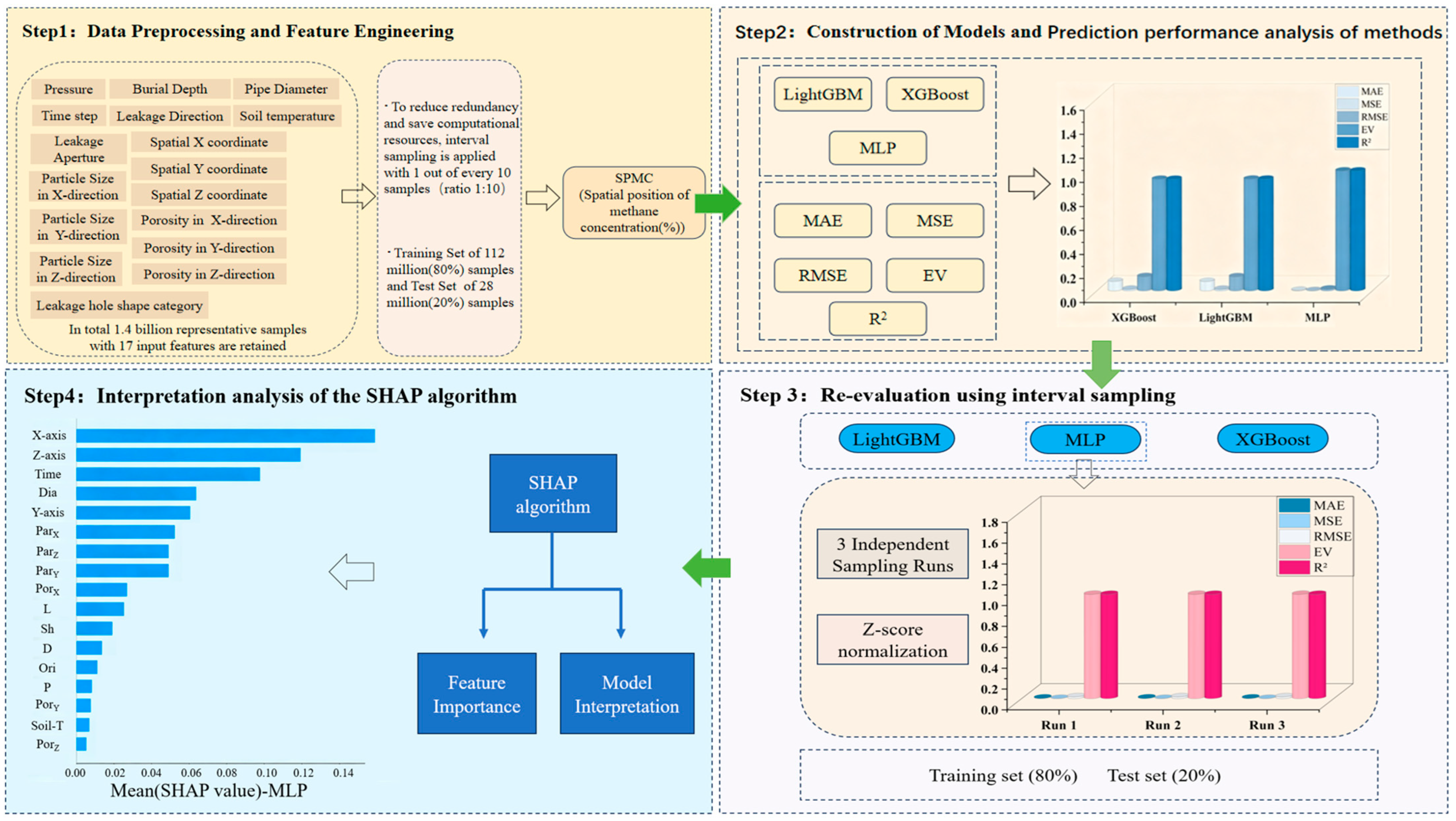
To systematically carry out research on buried-pipeline leakage parameter prediction, this paper constructs an overall methodological framework of “numerical simulation–data processing–model construction–performance evaluation–result interpretation”. First, a CFD-based buried-pipeline leakage simulation model considering the influence of soil anisotropy is established to obtain leakage response data under different working conditions and form a sample database required for subsequent machine learning modeling. Second, preprocessing and feature engineering are performed on the simulation data, including sample sorting, missing value processing, feature extraction, normalization and dataset division, to improve the quality of input data and model training efficiency. On this basis, various machine learning models, including LightGBM, XGBoost and MLP, are constructed, and the performance of each model is comprehensively compared using indicators such as MAE, MSE, RMSE, R² and EV to screen out the model with better prediction effect. Finally, the SHAP method is applied to conduct interpretability analysis on the optimal model, revealing the contribution direction and influence degree of different input features to the leakage parameter prediction results, so as to realize the mechanism interpretation of model prediction results and the identification of key influencing factors. Based on the above steps, this paper forms a complete method system for rapid prediction and interpretive analysis of buried-pipeline leakage, providing methodological support for subsequent result discussion and engineering application. As illustrated in Figure 1, the overall methodology consists of four main stages: numerical simulation (CFD data generation), data processing (interval sampling and feature engineering), model construction (LightGBM, XGBoost, and MLP training and comparison), and result interpretation (SHAP analysis for both global and local interpretability). The research methodology process is shown in Figure 1.

2.1. Machine Learning Prediction Models

2.1.1. LightGBM

LightGBM is an ensemble learning method based on gradient boosting decision trees. Its core lies in adopting a histogram-based decision tree construction method, combined with two mechanisms—Gradient-based One-Side Sampling (GOSS) and Exclusive Feature Bundling (EFB)—which improve training efficiency while maintaining high prediction accuracy, making it more suitable for processing data with high-dimensional, nonlinear and obvious structural features [29]. For the problem of buried-pipeline leakage, leakage identification usually relies on multi-dimensional features extracted from pressure, flow rate, vibration or other monitoring responses. Such data often have complex coupling, noise interference and nonlinear mapping relationships; from recent pipeline research, LightGBM has been used for rapid risk assessment of oil- and gas-gathering pipeline leakage failure, as well as leakage location and leakage rate identification of drainage pipelines, indicating that this method has good applicability in processing structural features related to pipeline leakage [30,31]. Therefore, compared with complex deep networks with high computational cost, LightGBM is more suitable as an efficient prediction model in buried-pipeline leakage identification and risk discrimination, and can be further combined with feature importance or SHAP analysis to identify key leakage indicators.

The prediction result of LightGBM can be expressed as the accumulation of multiple weak learners, namely,

$${\widehat{y}}_i={\displaystyle \sum _{k=1}^K}{f}_k(x_i),f_k\in \mathcal{F}$$

(1)

where ${\hat{y}}_i$ is the predicted value of the $\mathrm{i}$-th sample, $x_i$ is the input feature, $f_k$ represents the $\mathrm{k}$-th decision tree, $\mathrm{F}$ is the regression tree space, and $\mathrm{K}$ is the total number of trees.

This formula shows that LightGBM gradually improves prediction ability through iterative superposition of multiple trees. In the $\mathrm{t}$-th iteration, the objective function of the model can be written as

$${\mathrm{O}\mathrm{b}\mathrm{j}}^{\left(t\right)}={\displaystyle \sum _{i=1}^n}l\left(y_i,{\widehat{y}}_i^{\left(t−1\right)}+f_t(x_i)\right)+\mathrm{\Omega }(f_t)$$

(2)

where $l(·)$ is the loss function, $y_i$ is the true value, ${\hat{y}}_i^{(t-1)}$ is the prediction result of the model in the first $\mathrm{t}-1$ rounds, $f_t\left(x_i\right)$ is the output of the newly added tree in the current round, and $\mathrm{\Omega }\left(f_t\right)$ is the regularization term used to control model complexity.

The regularization term is usually written as

$$\mathrm{\Omega }(f_t)=\gamma T+{\displaystyle \frac{1}{2}}\lambda {\displaystyle {\sum }_{j=1}^T}{w}_j^2$$

(3)

where $T$ is the number of leaf nodes, $w_j$ is the weight of the $\mathrm{j}$-th leaf node, and $\gamma$ and $\lambda$ are regularization parameters. This term is used to suppress model overfitting and improve generalization ability.

For the convenience of the solution, the objective function is usually expanded by a second-order Taylor series to obtain

$${\mathrm{O}\mathrm{b}\mathrm{j}}^{\left(t\right)}\approx {\displaystyle {\sum }_{i=1}^n}\left[g_i{f}_t(x_i)+{\displaystyle \frac{1}{2}}{h}_i{f}_t^2(x_i)\right]+\mathrm{\Omega }(f_t)$$

(4)

where

$$g_i={\displaystyle \frac{\partial l(y_i,{\widehat{y}}_i^{\left(t−1\right)})}{\partial {\widehat{y}}_i^{\left(t−1\right)}}},h_i={\displaystyle \frac{{\partial }^{2}l(y_i,{\widehat{y}}_i^{\left(t−1\right)}{)}^2}{\partial ({\widehat{y}}_i^{\left(t−1\right)}{)}^2}}$$

(5)

represent the first-order and second-order derivatives of the loss function with respect to the predicted value, respectively. LightGBM constructs each newly added decision tree based on this information. For tree node splitting, the commonly used splitting gain of LightGBM can be expressed as

$$\mathrm{G}\mathrm{a}\mathrm{i}\mathrm{n}={\displaystyle \frac{1}{2}}\left({\displaystyle \frac{G_L^2}{H_L+\lambda }}+{\displaystyle \frac{G_R^2}{H_R+\lambda }}-{\displaystyle \frac{\left(G_L+G_R{)}^2\right.}{H_L+H_R+\lambda }}\right)-\gamma$$

(6)

where $G_L$ and $G_R$ represent the sum of first-order gradients of samples in the left and right child nodes respectively, $H_L$ and $H_R$ represent the sum of second-order gradients of samples in the left and right child nodes respectively, and $\lambda$ and $\gamma$ are regularization parameters. The larger the splitting gain, the better the current division method.

2.1.2. eXtreme Gradient Boosting (XGBoost)

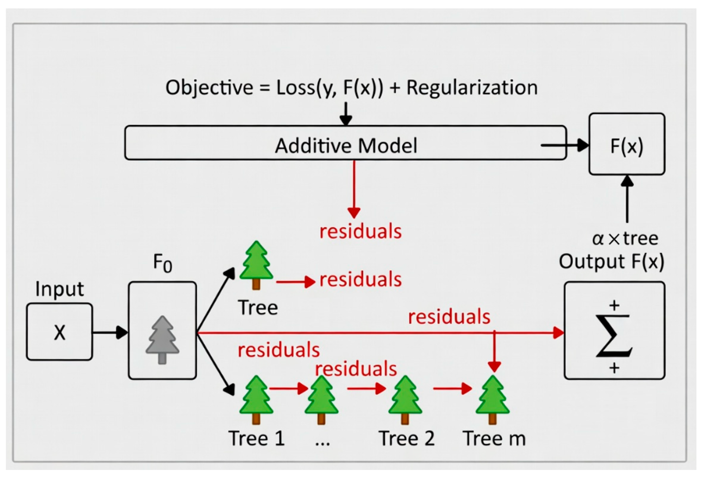
XGBoost is an ensemble learning method based on gradient boosting trees. Its core idea is to gradually construct new decision trees to fit the residuals of the previous round of models, and introduce regularization terms into the objective function to improve prediction accuracy and suppress overfitting, so it has strong advantages in dealing with nonlinear relationships and multi-factor coupling problems [32]. For the problem of buried-pipeline leakage, leakage monitoring data usually comes from signals such as pressure, vibration, acoustics or flow rate. These signals are susceptible to attenuation, noise interference and environmental factors when propagating in soil media, resulting in nonlinear, coupled and unstable leakage characteristics [21]. Compared with network models that rely more on long-term sequence modeling capabilities, XGBoost is more suitable for learning extracted structural features. It can not only characterize the complex mapping relationship between various influencing factors and leakage status, but also output feature importance, facilitating the identification of key leakage indicators, so it is suitable for buried-pipeline leakage identification and risk discrimination [33]. The XGBoost principle is shown in Figure 2. Black arrows indicate the forward prediction flow, and red arrows indicate the residuals fitted by newly added regression trees.

Mathematically, XGBoost expresses the sample predicted value as the accumulation of outputs from multiple regression trees, namely,

$${\widehat{\mathrm{y}}}_{\mathrm{i}}={\displaystyle \sum _{\mathrm{k}=1}^{\mathrm{K}}}{\mathrm{f}}_{\mathrm{k}}({\mathrm{x}}_{\mathrm{i}}),{\mathrm{f}}_{\mathrm{k}}\in \mathcal{F}$$

(7)

Its objective function can be written as

$${\mathrm{O}\mathrm{b}\mathrm{j}}^{\left(\mathrm{t}\right)}={\displaystyle \sum _{\mathrm{i}=1}^{\mathrm{n}}}\mathrm{l}\left({\mathrm{y}}_{\mathrm{i}},{\widehat{\mathrm{y}}}_{\mathrm{i}}^{\left(\mathrm{t}−1\right)}+{\mathrm{f}}_{\mathrm{t}}({\mathrm{x}}_{\mathrm{i}})\right)+\mathrm{\Omega }({\mathrm{f}}_{\mathrm{t}})$$

(8)

where $\mathrm{\Omega }\left(f_t\right)$ is the regularization term, usually expressed as

$$\mathrm{\Omega }({\mathrm{f}}_{\mathrm{t}})=\mathrm{\gamma }\mathrm{T}+{\displaystyle \frac{1}{2}}\mathrm{\lambda }{\displaystyle \sum _{\mathrm{j}=1}^{\mathrm{T}}}{\mathrm{w}}_{\mathrm{j}}^2$$

(9)

To improve solution efficiency, XGBoost expands the objective function by a second-order Taylor series to obtain

$${\mathrm{O}\mathrm{b}\mathrm{j}}^{\left(\mathrm{t}\right)}\approx {\displaystyle \sum _{\mathrm{i}=1}^{\mathrm{n}}}\left[{\mathrm{g}}_{\mathrm{i}}{\mathrm{f}}_{\mathrm{t}}({\mathrm{x}}_{\mathrm{i}})+{\displaystyle \frac{1}{2}}{\mathrm{h}}_{\mathrm{i}}{\mathrm{f}}_{\mathrm{t}}^2({\mathrm{x}}_{\mathrm{i}})\right]+\mathrm{\Omega }({\mathrm{f}}_{\mathrm{t}})$$

(10)

where $g_i$ and $h_i$ represent the first-order and second-order derivatives of the loss function with respect to the predicted value, respectively. It can be seen that XGBoost achieves the unity of prediction accuracy and generalization ability through the combination of residual iterative fitting and regularization constraints.

2.1.3. Multi-Layer Perceptron (MLP)

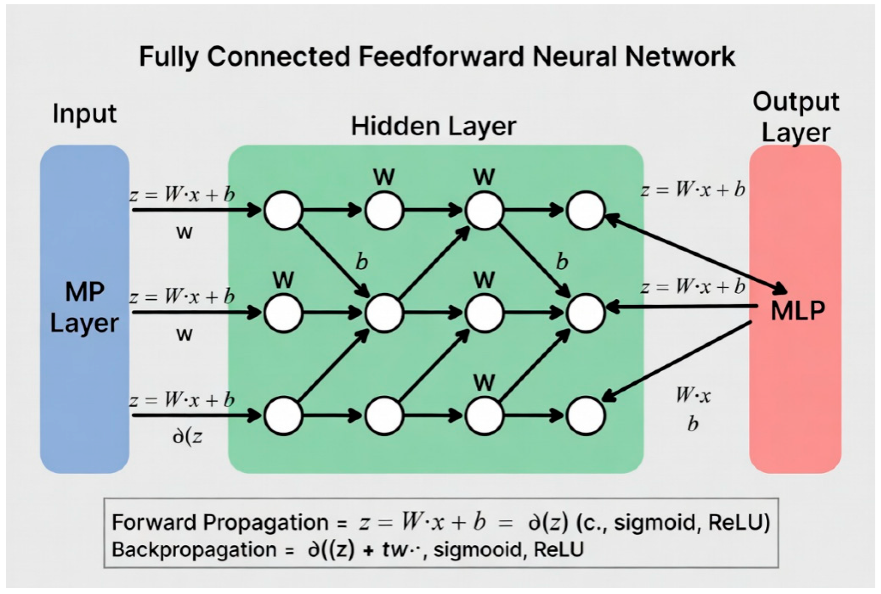
MLP is a typical feedforward artificial neural network. Its basic structure consists of an input layer, one or more hidden layers, and an output layer. It performs nonlinear mapping of input features through fully connected layers and supervised learning mechanisms, so it can well fit complex multivariate relationships [34]. For the problem of buried-pipeline leakage, leakage monitoring signals usually come from vibration, pressure or acoustic responses. These signals are prone to attenuation, distortion and fluctuation under the action of soil media and environmental noise, so noise reduction, feature extraction and structural expression are often required in actual modeling [19]. In this case, MLP can directly learn the nonlinear mapping relationship between extracted features and leakage status, and has a relatively simple model structure with fast training and inference speed, so it is suitable for buried-pipeline leakage identification and status discrimination [21]. The MLP principle is shown in Figure 3.

Let the input sample be

$$\mathrm{x}=[{\mathrm{x}}_1,{\mathrm{x}}_2,\dots ,{\mathrm{x}}_{\mathrm{n}}{]}^{\mathrm{T}}$$

(11)

Then the output of the $\mathrm{l}$-th neural network layer can be expressed as

$${\mathrm{h}}^{\left(\mathrm{l}\right)}=\mathrm{\varphi }\left({\mathrm{W}}^{\left(\mathrm{l}\right)}{\mathrm{h}}^{\left(\mathrm{l}−1\right)}+{\mathrm{b}}^{\left(\mathrm{l}\right)}\right)$$

(12)

where $h^{(l-1)}$ is the output of the $(\mathrm{l}-1)$-th layer, $W^{\left(l\right)}$ and $b^{\left(l\right)}$ are the weight matrix and bias vector of the $\mathrm{l}$-th layer respectively, and $\mathrm{\varphi }(·)$ is the activation function. For the input layer,

$${\mathrm{h}}^{\left(0\right)}=\mathrm{x}$$

(13)

If the output layer is used for regression prediction, the final output of the model can be written as

$$\widehat{\mathrm{y}}={\mathrm{W}}^{\left(\mathrm{L}\right)}{\mathrm{h}}^{\left(\mathrm{L}−1\right)}+{\mathrm{b}}^{\left(\mathrm{L}\right)}$$

(14)

where $\hat{y}$ is the predicted value and $L$ is the total number of network layers. It can be seen that MLP gradually extracts features through multi-layer mapping and converts input variables into target outputs. Its training process usually aims to minimize the loss function. For regression problems, mean squared error is often used as the loss function, namely,

$$\mathcal{L}={\displaystyle \frac{1}{\mathrm{N}}}{\displaystyle \sum _{\mathrm{i}=1}^{\mathrm{N}}}({\mathrm{y}}_{\mathrm{i}}-{\widehat{\mathrm{y}}}_{\mathrm{i}}{)}^2$$

(15)

where $y_i$ is the true value, ${\hat{y}}_i$ is the predicted value, and $N$ is the number of samples. During training, MLP uses the backpropagation algorithm to calculate the gradient of the loss function with respect to each layer parameter, and iteratively updates the weights and biases combined with gradient descent or its improved algorithms, so as to continuously improve prediction accuracy. The above training mechanism of “forward propagation + error backpropagation” is also the core of MLP’s ability to learn complex nonlinear mapping relationships.

2.2. Interpretability Analysis Method

To better explain the reasons behind model predictions and enhance model interpretability, this paper adopts the SHAP algorithm to interpret the model, understand the reasons for model predictions, and enhance the interpretability of model prediction results.

SHAP is a model interpretation method based on cooperative game theory, used to quantify the contribution of each input feature to the model prediction result. Its core idea is to calculate the marginal contribution of features to the model output under different combinations to obtain the corresponding Shapley value, so as to realize interpretable analysis of model prediction results [35]. The recent perspective by Salih et al. systematically discusses SHAP and LIME as representative explainable artificial intelligence methods, highlighting the value of such methods in improving the transparency and trustworthiness of complex machine learning models. Compared with traditional feature importance methods, SHAP can provide both local and global interpretations: on the one hand, it can explain how each feature in a single sample pushes the prediction result up or down; on the other hand, it can sort the overall feature importance by summarizing the SHAP values of multiple samples. Due to its unified additive expression form, SHAP has become one of the most widely used methods in the interpretation of tabular data models [36].

The additive interpretation model of SHAP is usually expressed as

$$\mathrm{g}({\mathrm{z}}^{\prime })={\mathrm{\varphi }}_0+{\displaystyle \sum _{\mathrm{i}=1}^{\mathrm{M}}}{\mathrm{\varphi }}_{\mathrm{i}}{\mathrm{z}}_{\mathrm{i}}^{\prime }$$

(16)

where $g\left(z^{\prime }\right)$ is the output of the interpretation model, ${\varphi }_0$ is the base value, ${\varphi }_i$ is the SHAP value corresponding to the $\mathrm{i}$-th feature, and $z_i^{\prime }$ indicates whether the feature participates in the current interpretation. This formula shows that the model prediction result can be decomposed into the sum of the base output and the contribution of each feature.

For the $\mathrm{i}$-th feature, its Shapley value can be written as

$${\mathrm{\varphi }}_{\mathrm{i}}=\sum _{\mathrm{S}\subseteq \mathrm{F}\setminus \left\{\mathrm{i}\right\}}{\displaystyle \frac{\mid \mathrm{S}\mid !(\mathrm{M}-\mid \mathrm{S}\mid -1)!}{\mathrm{M}!}}\left[{\mathrm{f}}_{\mathrm{S}\cup \left\{\mathrm{i}\right\}}\left(\mathrm{x}\right)-{\mathrm{f}}_{\mathrm{S}}\left(\mathrm{x}\right)\right]$$

(17)

where $F$ is the set of all features, $S$ is any subset of features not including feature $\mathrm{i}$, $M$ is the total number of features, and $f_S\left(x\right)$ represents the model output when only feature subset $\mathrm{S}$ is considered. This formula reflects the average marginal contribution of feature $\mathrm{i}$ in all possible feature combinations, so it can fairly measure the impact of each feature on the prediction result.

2.3. Model Evaluation Metrics

(1)

Mean Absolute Error (MAE)

$$\mathrm{M}\mathrm{A}\mathrm{E}={\displaystyle \frac{1}{\mathrm{n}}}{\displaystyle \sum _{\mathrm{i}=1}^{\mathrm{n}}}\mid {\mathrm{y}}_{\mathrm{i}}-{\widehat{\mathrm{y}}}_{\mathrm{i}}\mid$$

(18)

where $n$ represents the number of samples, $y_i$ represents the true value of the $\mathrm{i}$-th sample, and ${\widehat{y}}_i$ represents the predicted value of the $\mathrm{i}$-th sample.

MAE represents the average level of absolute errors between predicted and true values, and can directly reflect the overall prediction deviation of the model. The smaller the value, the closer the model prediction result is to the true value. Due to the use of absolute value, MAE is relatively less sensitive to outliers.

(2)

Mean Squared Error (MSE)

$$\mathrm{M}\mathrm{S}\mathrm{E}={\displaystyle \frac{1}{\mathrm{n}}}{\displaystyle \sum _{\mathrm{i}=1}^{\mathrm{n}}}{\left({\mathrm{y}}_{\mathrm{i}}−{\widehat{\mathrm{y}}}_{\mathrm{i}}\right)}^2$$

(19)

MSE represents the average value of squared prediction errors, used to measure the deviation between model prediction results and true values. Since errors are amplified by squaring, MSE is more sensitive to large errors and outliers, so it is often used in scenarios that emphasize large deviation penalties. The smaller the MSE value, the better the model prediction performance.

(3)

Root Mean Squared Error (RMSE)

$$\mathrm{R}\mathrm{M}\mathrm{S}\mathrm{E}=\sqrt{{\displaystyle \frac{1}{\mathrm{n}}}{\displaystyle \sum _{\mathrm{i}=1}^{\mathrm{n}}}{\left({\mathrm{y}}_{\mathrm{i}}−{\widehat{\mathrm{y}}}_{\mathrm{i}}\right)}^2}$$

(20)

RMSE is the result of MSE after square root extraction, used to reflect the overall level of prediction errors. Compared with MSE, RMSE has the same dimension as the original data, so it is more convenient for direct comparison with physical quantities in practical problems. The smaller the RMSE, the higher the model prediction accuracy; meanwhile, it is still sensitive to large errors.

(4)

R-squared (${\mathrm{R}}^2$)

$${\mathrm{R}}^2=1-{\displaystyle \frac{{\displaystyle {\sum }_{\mathrm{i}=1}^{\mathrm{n}}}({\mathrm{y}}_{\mathrm{i}}-{\widehat{\mathrm{y}}}_{\mathrm{i}}{)}^2}{{\displaystyle {\sum }_{\mathrm{i}=1}^{\mathrm{n}}}({\mathrm{y}}_{\mathrm{i}}-\stackrel{\mathrm{ˉ}}{\mathrm{y}}{)}^2}}$$

(21)

${\mathrm{R}}^2$ is used to measure the fitting degree of the model to the variation law of real data, that is, the proportion of dependent variable variation that the model can explain. Its value is usually between 0 and 1, and the closer to 1, the better the fitting effect; when ${\mathrm{R}}^2=1$, it means that the predicted value is completely consistent with the true value; when ${\mathrm{R}}^2=0$, it means that the model prediction effect is equivalent to direct prediction using the mean value; in some cases, ${\mathrm{R}}^2$ may also be less than 0, indicating poor model performance.

(5)

Explanatory Variance (EV)

$$\mathrm{E}\mathrm{V}=1-{\displaystyle \frac{\mathrm{V}\mathrm{a}\mathrm{r}(\mathrm{y}-\widehat{\mathrm{y}})}{\mathrm{V}\mathrm{a}\mathrm{r}\left(\mathrm{y}\right)}}$$

(22)

where $Var(y-\widehat{y})$ represents the variance of prediction residuals, and $Var\left(y\right)$ represents the variance of true values.

EV is used to measure the model’s ability to explain the fluctuation characteristics of real data, that is, the degree to which the model can explain the variance of true values. The closer EV is to 1, the more effectively the model can reflect the change trend of real data; when EV equals 1, it means that the prediction result is completely consistent with the true value; if EV is small or even negative, it means that the model’s ability to explain data fluctuations is weak.

3. Model Training and Result Analysis

This section presents the training and evaluation results of the machine learning models for buried-pipeline leakage concentration prediction.

3.1. Model Parameter Settings

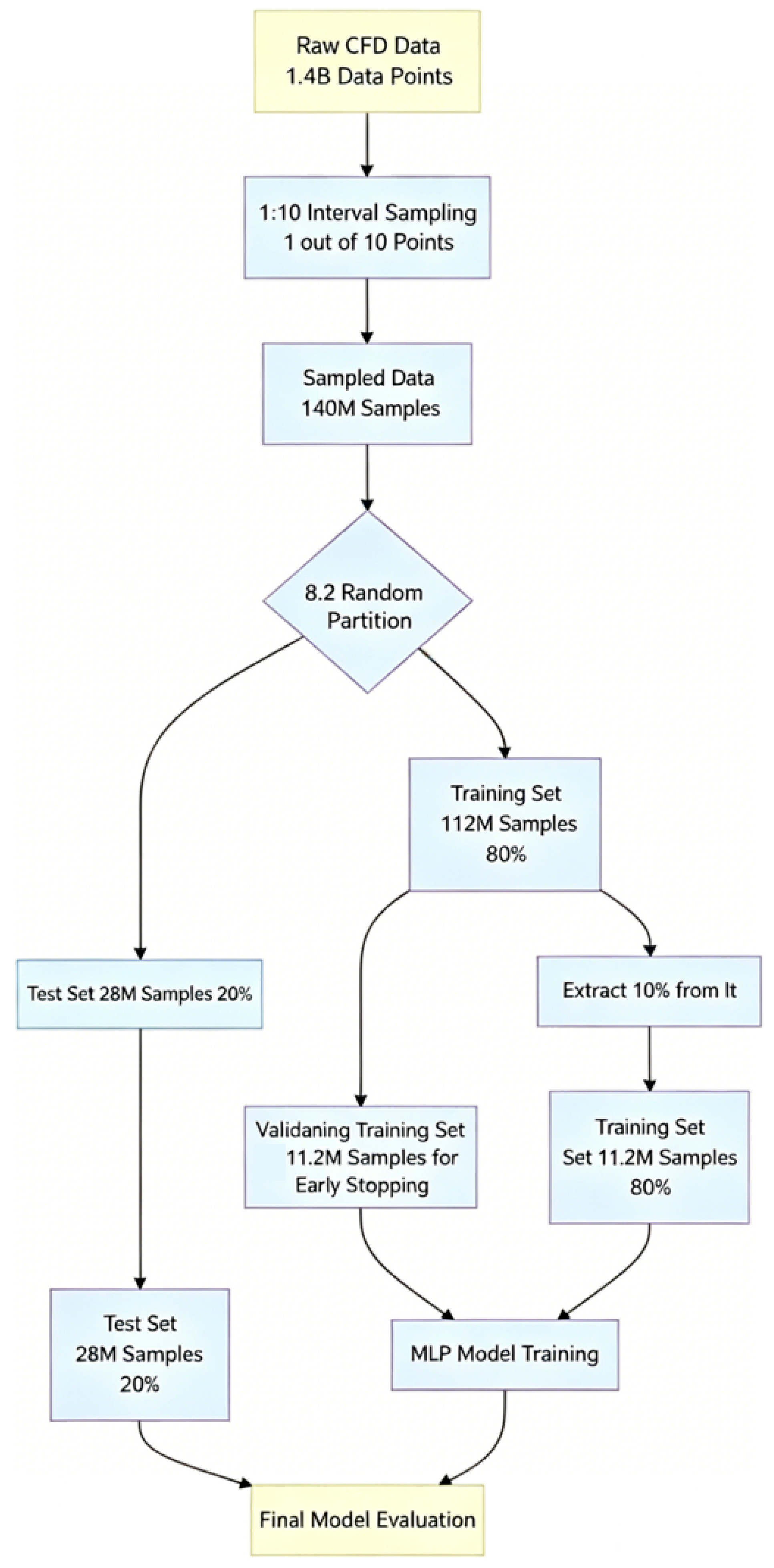
The total amount of original CFD simulation data in this study is 1.4 billion, including leakage concentration distribution under different leakage conditions, spatial positions and time steps. Considering that the original data has strong temporal and spatial continuity, and the feature changes between adjacent samples are small, direct use of all data will introduce a large amount of redundant information and significantly increase training time and storage overhead. To this end, this study adopts an interval sampling strategy: along the data generation order (i.e., the sequence of CFD simulation outputs over time and spatial coordinates), retaining one out of every 10 data points along the data generation order—that is, the sampling ratio is 1:10—and finally, 140 million representative samples are obtained. The 1:10 ratio was chosen to balance computational feasibility with information preservation—reducing data volume by an order of magnitude while retaining key features. The reliability of the CFD simulation data has been validated through grid independence tests and comparison with experimental data in our previous work [37,38]. Then, the samples are randomly divided into a training set (112 million) and a test set (28 million) at a ratio of 8:2.

There are 17 dimensions of input features, with detailed descriptions shown in

Table 1. Description of input features.

No.	Feature Name	Unit/Description
1	P	MPa/Pressure
2	D	mm/Pipe Diameter
3	L	m/Burial Depth
4	Dia	mm/Leakage Aperture
5	Sh	Dimensionless/Leakage Hole Shape Category
6	Ori	Dimensionless/Leakage Direction
7	PorX	Dimensionless/Porosity in X-Direction
8	ParX	μm/Particle Size in X-Direction
9	PorY	Dimensionless/Porosity in Y-Direction
10	ParY	μm/Particle Size in Y-Direction
11	PorZ	Dimensionless/Porosity in Z-Direction
12	ParZ	μm/Particle Size in Z-Direction
13	Soil-T	°C/Soil Temperature
14	Time	Dimensionless/Time Step
15	X-axis	Dimensionless/Spatial X Coordinate
16	Y-axis	Dimensionless/Spatial Y Coordinate
17	Z-axis	Dimensionless/Spatial Z Coordinate

. For the categorical features Sh (leakage hole shape: circle, square, rectangle, triangle) and Ori (leakage direction: up, down, left, right), one-hot encoding was applied to avoid introducing any artificial ordinal relationship. The prediction target is Spatial Position of Methane Concentration (SPMC, %). This Multi-Layer Perceptron (MLP) employs the structure and parameter configuration shown in

Table 2. MLP parameter settings.

Parameter	Value	Description
Hidden Layer Structure	[128, 64, 32]	Three fully connected layers
Activation Function	ReLU	Hidden layer
Output Layer Activation Function	Linear	Regression output
Dropout	0.2	Prevent overfitting
Batch Size	1024	Number of samples per batch
Epochs	100	Maximum training rounds
Optimizer	Adam	Adaptive learning rate
Initial Learning Rate	0.001	Fixed
Early Stopping	10 rounds	Stop when validation loss does not decrease
Loss Function	MSE	Mean squared error
Weight Initialization	Xavier	Stabilize training
random_state	42	Random seed

:

3.2. Model Performance Comparison

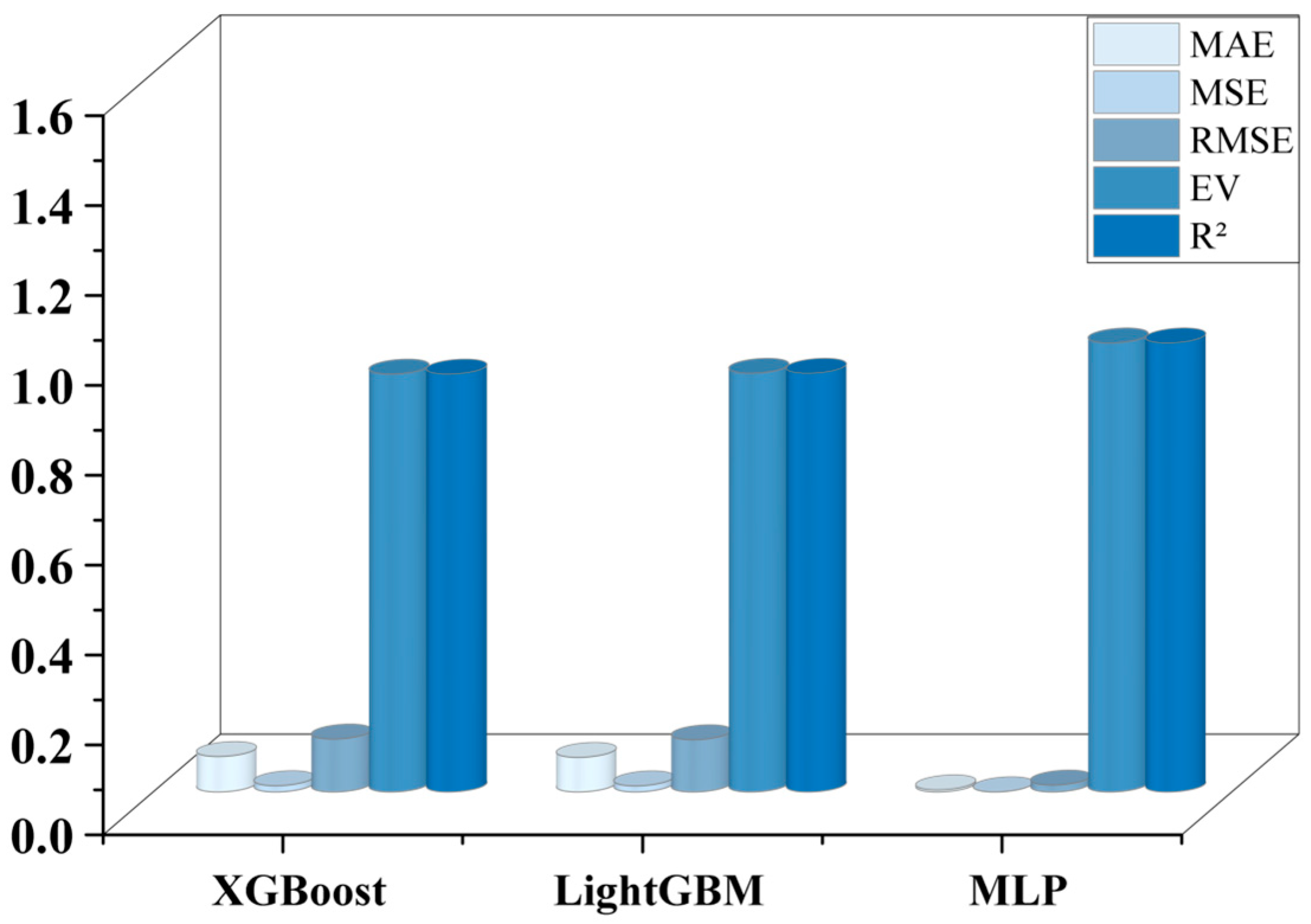
The overall data processing and model training procedure is illustrated in Figure 4. This study selects the XGBoost, LightGBM and MLP models for the leakage concentration prediction task. XGBoost and LightGBM adopt default parameter configurations, and MLP adopts the parameters shown in Table 2. The three models are trained on the same training set (112 million samples) and evaluated on the test set (28 million samples), with the results shown in Figure 5.

As shown in Figure 5, MLP is significantly superior to the two tree-based models in all indicators, with an ${\mathrm{R}}^2$ of 0.9988 and an RMSE of only 0.0153, indicating that the deep neural network can more effectively capture the complex nonlinear relationship between leakage concentration and 17 dimensions of input features. LightGBM and XGBoost have similar performance, with an ${\mathrm{R}}^2$ of about 0.93, both having good prediction ability, but there is an order-of-magnitude error gap compared with MLP. This superior performance of MLP can be attributed to three main factors: (1) a large-scale high-fidelity CFD dataset containing 1.4 billion original data points, (2) an effective 1:10 interval sampling strategy that preserves key information while reducing data volume, and (3) the strong capability of MLP to capture complex nonlinear mappings. While CFD simulations provide high-fidelity physical insights, they are computationally expensive and unsuitable for real-time applications. The computational cost of the MLP model is as follows: data loading took 4.46 min, data splitting took 2.59 min, and model training on seven NVIDIA RTX 4090 GPUs with 512 GB system memory took approximately 12 min. Once trained, the inference time for a single new sample is on the order of milliseconds, and batch inference on the 28 million test samples can be completed within minutes. In contrast, a single CFD simulation under the same conditions requires several hours.

3.3. Interval Sampling of the Optimal Model

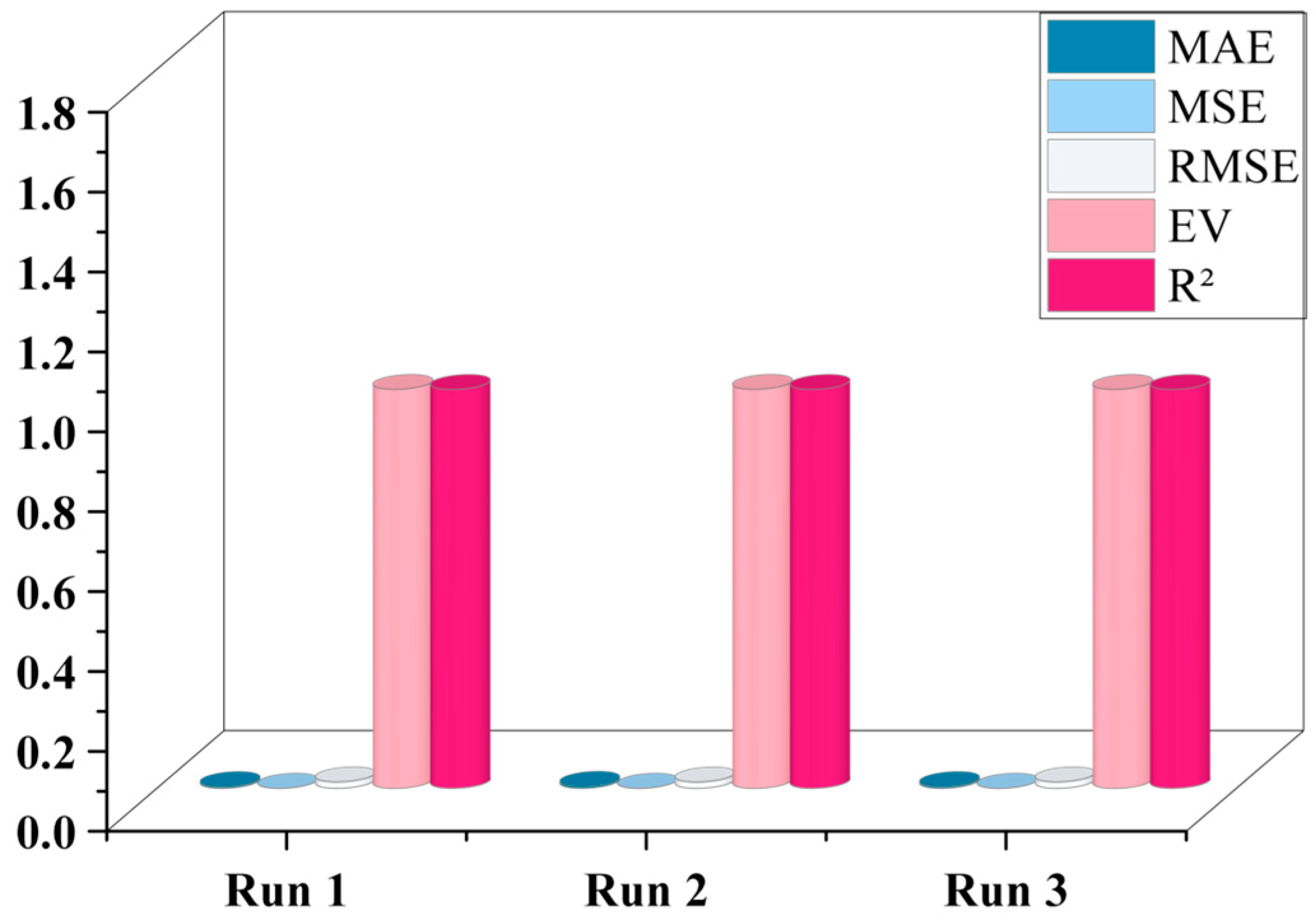
Based on the 140 million samples obtained by the above interval sampling, the dataset is divided into a training set (112 million) and a test set (28 million) at a ratio of 8:2. To comprehensively evaluate the sensitivity and generalization ability of the optimal model (MLP) to different sampling starting points, this study designed three independent repeated experiments. Each experiment adopts different sampling starting offsets (offset = 0, 1, 2), that is, sampling one out of every 10 data points starting from the first, second, and third data points of the original 1.4 billion data respectively. The model structure and hyperparameters of the three experiments remain completely consistent, with only minor differences in training data. The evaluation results of the three independent repeated experiments on the test set are shown in Figure 6.

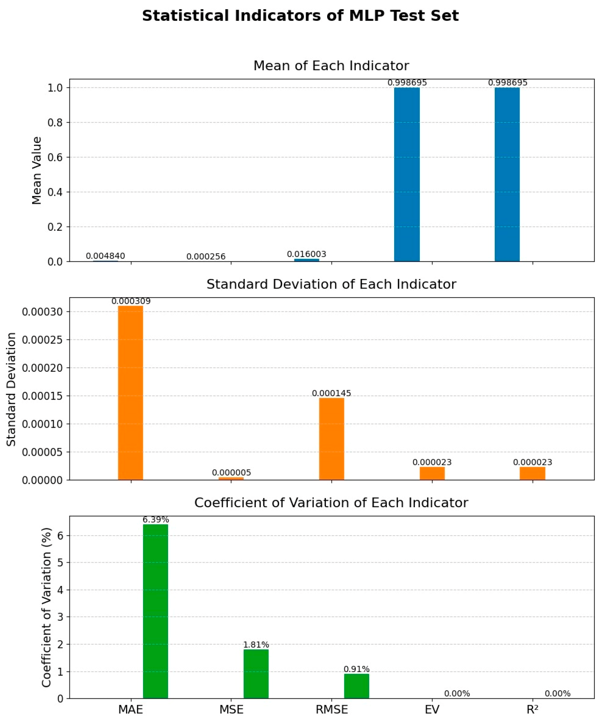
Statistical description is performed on the test set results of the three experiments, and the mean, standard deviation and coefficient of variation (ratio of standard deviation to mean) are calculated, with the results shown in Figure 7.

It can be seen from Figure 6 and Figure 7 that the ${\mathrm{R}}^2$ of all three experiments reaches about 0.9987, the RMSE is stable at around 0.0160, and the EV for all is close to 0.9987, indicating that MLP can stably and accurately fit the complex nonlinear mapping relationship between leakage concentration and 17 dimensions of input features, and the model has a strong ability to explain data variance. From the statistical indicators, the standard deviation of ${\mathrm{R}}^2$ and EV is only 0.000023 with a coefficient of variation of 0.00%, the coefficient of variation in RMSE is 0.91%, and the coefficient of variation in MAE is 6.39%, all at a low level, proving that MLP is insensitive to different sampling starting points and has good repeatability and robustness. Comprehensive comparison of the three experiments: Run 2 achieves the highest ${\mathrm{R}}^2$ (0.998727) and the lowest RMSE (0.015798), which is the optimal accuracy model; Run 1 achieves the lowest MAE (0.004585), which is the optimal absolute deviation model, which can be selected according to specific needs in practical applications. In addition, the performance fluctuations of the three experiments are minimal, indicating that the 1:10 equal interval sampling can fully retain the effective information of the original 1.4 billion data points, and the sampling process does not introduce significant information loss or distribution shift, verifying the effectiveness and reliability of interval sampling as a large-scale CFD data dimensionality reduction strategy.

3.4. SHAP Interpretability Analysis

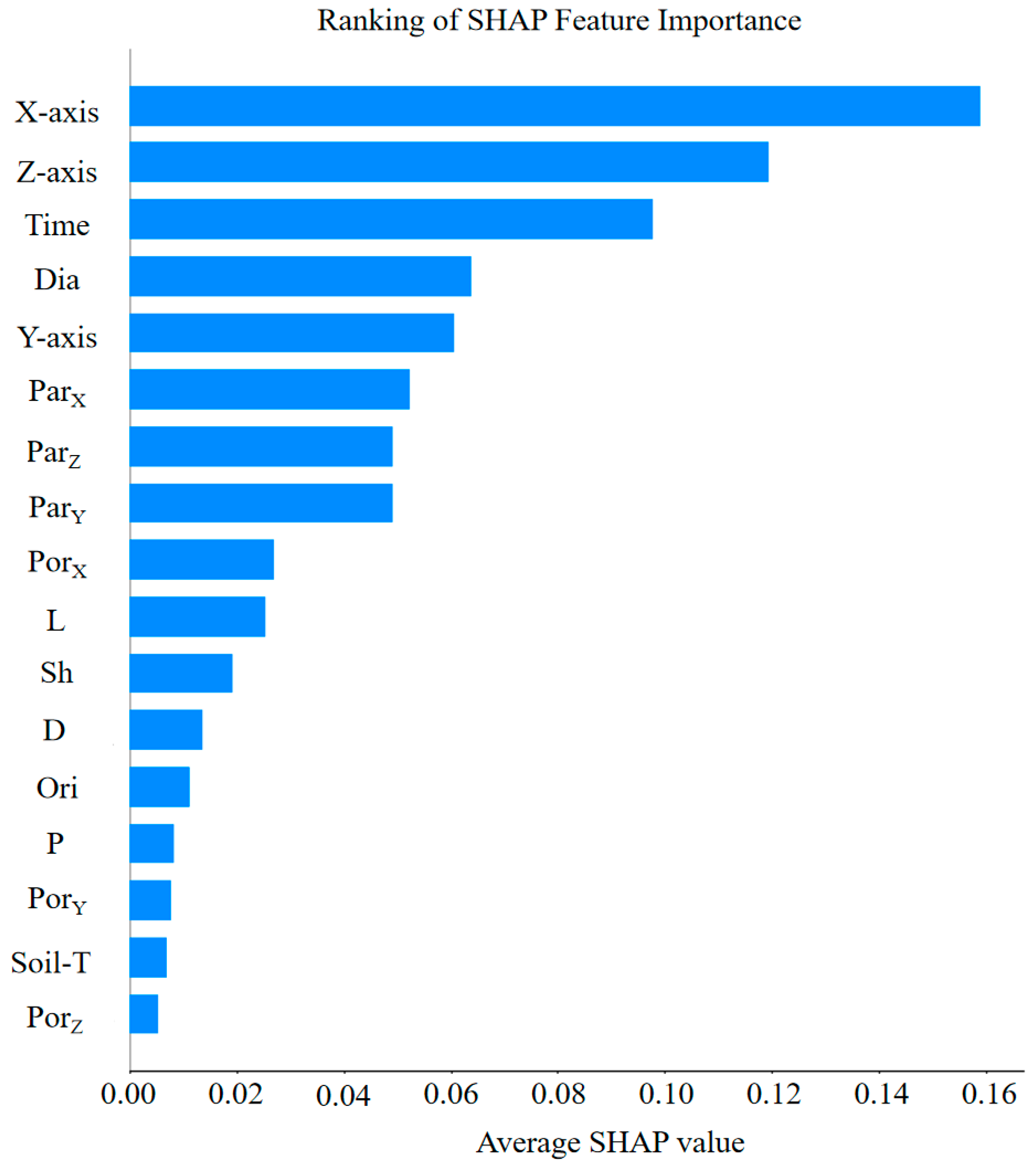
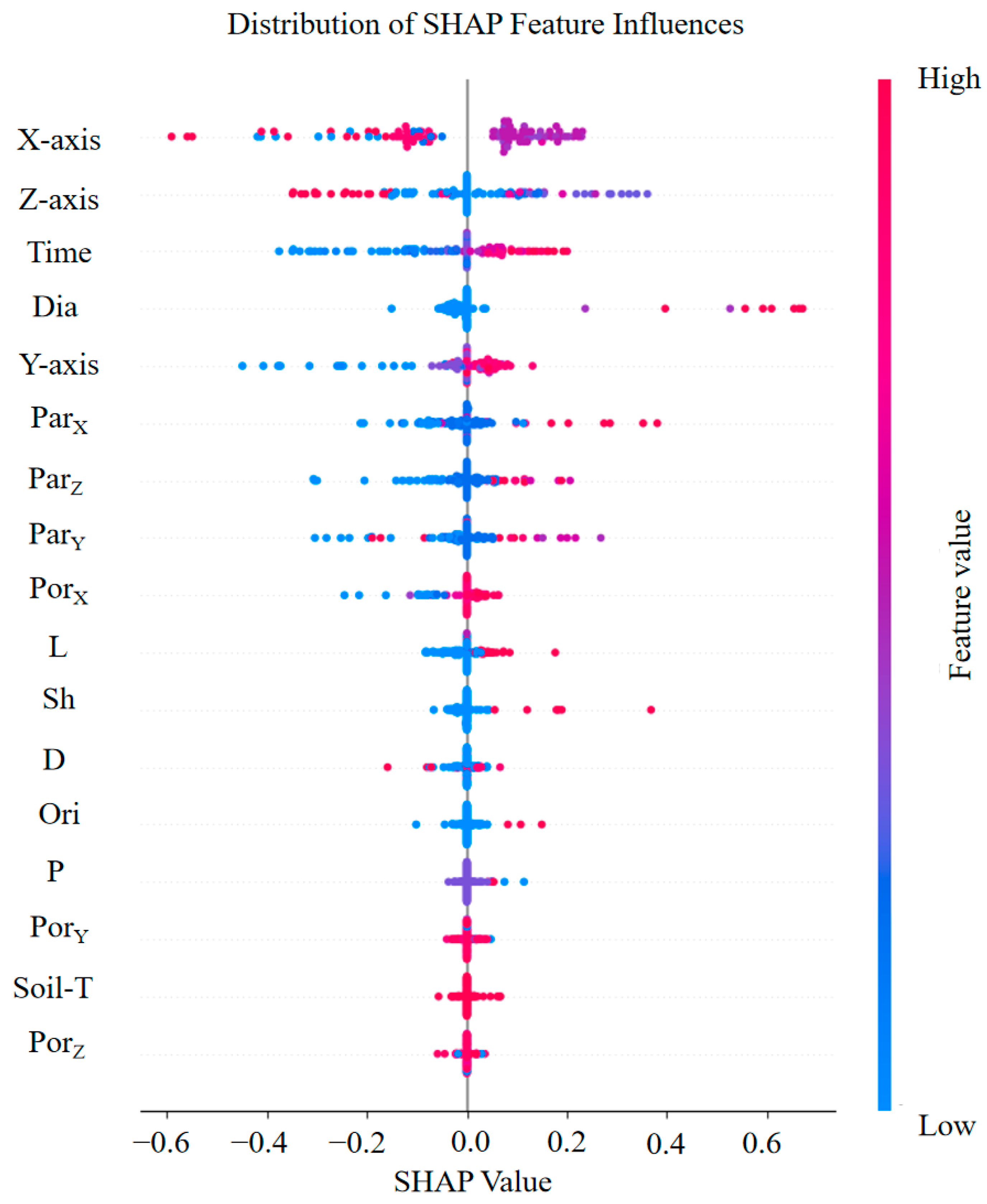
To reveal the decision-making basis of the machine learning model in the prediction of buried-pipeline leakage concentration, this study adopts the SHAP method to conduct interpretability analysis on the optimal model. The SHAP value reflects the marginal contribution of each feature to the model prediction result, and the larger its absolute value, the more significant the influence of the feature on the prediction result. The SHAP values of each input feature are calculated based on the MLP model, and the feature importance ranking is obtained by averaging the absolute values according to feature dimensions, as shown in Figure 8. Figure 9 shows the detailed distribution of SHAP values of each feature (beeswarm plot), where each point represents a sample, the color indicates the level of the feature value (red for high value, blue for low value), and the horizontal axis position indicates the positive or negative contribution of the feature to the predicted concentration.

It can be seen from Figure 8 and Figure 9 that spatial position is the dominant factor affecting leakage concentration. The X-axis (SHAP = 0.16) and Z-axis (SHAP = 0.13) rank first and second respectively, much higher than other features. The SHAP values of high-value samples are mostly negative, and the SHAP values of low-value samples are mostly positive, indicating that positions closer to the leakage source correspond to higher predicted concentrations, and positions far from the leakage source correspond to lower predicted concentrations, which is consistent with the physical intuition of concentration attenuation with diffusion distance. The time feature also has an important influence, ranking third (SHAP = 0.09). The SHAP values of high-value samples are scattered, with both positive and negative contributions, indicating that the leakage concentration shows a non-monotonic change trend of first rising and then stabilizing with time. Among the leakage source parameters, aperture (SHAP = 0.04) ranks fourth, and the SHAP values of its high-value samples are mainly positive, indicating that a large aperture leads to a higher leakage rate and predicted concentration. The influence of particle size cannot be ignored. The particle sizes in the X-, Y- and Z-directions rank sixth, seventh and eighth respectively, with SHAP values between 0.025 and 0.035. Their SHAP value distribution shows a certain nonlinear characteristic: moderate particle size values contribute the most to concentration, while too small or too large particle sizes reduce the predicted concentration, reflecting the complex influence of particle size on gas diffusion paths. The differences in three-direction particle sizes also reflect the characteristics of soil anisotropy. In terms of porosity, PorX (SHAP = 0.02) ranks ninth, while the porosities in the Y- and Z-directions rank lower (SHAP ≤ 0.001), indicating that the porosity in the X-direction has a more prominent influence on concentration distribution within the data range of this study. The SHAP values of other features such as pipe diameter, direction, pressure and soil temperature are all lower than 0.005, with relatively limited contribution to leakage concentration prediction, possibly due to their variation ranges in the dataset being small, or their influences being covered by spatial position and time features.

In summary, spatial position (X, Z coordinates) and time are the key factors affecting leakage concentration, followed by aperture and particle size. This finding can provide theoretical guidance for the optimal layout of sensors in buried-pipeline leakage monitoring; that is, focus should be placed on the concentration gradient changes at different spatial positions near the leakage source, and the time evolution law should be considered.

4. Conclusions

Aiming at the problem of buried-pipeline leakage concentration prediction, this paper proposes a data-driven method based on MLP and interval sampling. Through large-scale CFD data modeling and interpretability analysis, high-precision prediction of leakage concentration and identification of key influencing factors are realized. The main conclusions are as follows:

(1)

Superiority of MLP for concentration regression: Among the models tested, MLP achieved the highest accuracy (R² = 0.9988, RMSE = 0.0153), demonstrating its superior capability to capture the complex, nonlinear mapping between multi-physical features (pressure, soil properties, spatial coordinates) and leakage concentration. This makes it a highly suitable surrogate model for CFD.

(2)

Validation of the 1:10 sampling strategy: Three independent repeated experiments proved that the 1:10 interval-sampling strategy effectively reduces data volume (from 1.4B to 140M) without compromising model performance. The resulting MLP model showed exceptional stability (R² ≈ 0.9987, CV ≈ 0%), confirming the strategy’s reliability for large-scale CFD data dimensionality reduction.

(3)

Physical interpretability via SHAP: The SHAP analysis quantitatively revealed that spatial location (X, Z) is the dominant factor, followed by time and leak aperture. Notably, soil particle size (X, Y, Z) exhibited nonlinear effects, with medium values maximizing predicted concentration, reflecting its complex influence on gas diffusion in anisotropic porous media.

In summary, the MLP prediction model proposed in this paper balances accuracy and efficiency, reducing CFD computational costs from hours to milliseconds (R² = 0.9988). SHAP analysis identifies spatial location and leak aperture as key factors, providing practical guidance for sensor placement near leak sources. This offers an effective technical means for intelligent early warning of buried-pipeline leakage.

Nevertheless, this study has limitations: first, the fixed sampling strategy could be replaced by adaptive sampling to improve data efficiency; second, the current single-output framework can be extended to multi-output prediction for concentration distribution and diffusion range; finally, the model lacks validation with field-measured data, which should be addressed through future pipeline leakage experiments. Additionally, the nonlinear coupling between particle size and leak aperture, and deeper integration of SHAP results with porous-media flow mechanics, warrant further investigation.

References

1. Mahmoud, A.A.; Hasan, R. A Comprehensive Survey on Pipeline Monitoring Technologies: Advancements, Challenges, Market Opportunities and Future Directions. J. Pipeline Sci. Eng. 2025; in press. [CrossRef]
2. Ma, Q.; Liang, W.; Zhou, P. A Review on Pipeline In-Line Inspection Technologies. Sensors 2025, 25, 4873. [Google Scholar] [CrossRef]
3. Wei, Q.; Zhou, P.; Shi, X. Assessing the congestion cost of gas pipeline between China and Russia. Energy Strategy Rev. 2024, 55, 101493. [Google Scholar] [CrossRef]
4. Gaurina-Međimurec, N.; Novak Mavar, K.; Simon, K.; Djerdji, F. Accidents in Oil and Gas Pipeline Transportation Systems. Energies 2025, 18, 4056. [Google Scholar] [CrossRef]
5. Bu, F.; Lu, Q.; Jia, B.; Gao, X.; Zhang, H.; Wang, W.; Wang, Z. A Review of Research on Leakage and Diffusion Characteristics of Buried Gas Pipelines. J. Pipeline Sci. Eng. 2025; in press. [CrossRef]
6. Feng, Y.; Gao, J.; Yin, X.; Chen, J.; Wu, X. Risk assessment and simulation of gas pipeline leakage based on Markov chain theory. J. Loss Prev. Process Ind. 2024, 91, 105370. [Google Scholar] [CrossRef]
7. Xu, T.; Martynov, S.; Mahgerefteh, H. A Review of Optimization Methods for Pipeline Monitoring Systems: Applications and Challenges for CO2 Transport. Energies 2025, 18, 3591. [Google Scholar] [CrossRef]
8. Gong, Y.; Bao, C.; He, Z.; Jian, Y.; Wang, X.; Huang, H.; Song, X. A Review on Gas Pipeline Leak Detection: Acoustic-Based, OGI-Based, and Multimodal Fusion Methods. Information 2025, 16, 731. [Google Scholar] [CrossRef]
9. Abubakar, A.; Abisoye, O.A.; Alabi, I.O.; Solomon, A.; Oyefolahan, I.O. Systematic literature review and bibliometric analysis of pipeline monitoring and leakage detection techniques. Discov. Mech. Eng. 2025, 4, 17. [Google Scholar] [CrossRef]
10. Dai, Z.; Wang, T.; Hu, X.; Ma, D. A review of data-driven leakage diagnosis methods across pipeline and energy transportation system. J. Pipeline Sci. Eng. 2026; in press. [CrossRef]
11. Bagheri, M.; Sari, A. Study of natural gas emission from a hole on underground pipelines using optimal design-based CFD simulations: Developing comprehensive soil classified leakage models. J. Nat. Gas Sci. Eng. 2022, 102, 104583. [Google Scholar] [CrossRef]
12. Mohanty, S.; Brennan, S.; Molkov, V. CFD modelling of methane dispersion from buried pipeline leaks: Experimental validation and hazard distance estimation. Process Saf. Environ. Prot. 2024, 187, 1540–1557. [Google Scholar] [CrossRef]
13. Cai, Y.; Gu, X.; Zhang, X.; Zhang, K.; Zhang, H.; Xiong, Z. Acoustic Characterization of Leakage in Buried Natural Gas Pipelines. Processes 2025, 13, 2274. [Google Scholar] [CrossRef]
14. Chang, W.; Gu, X.; Zhang, X.; Gou, Z.; Zhang, X.; Xiong, Z. Numerical Study of the Soil Temperature Field Affected by Natural Gas Pipeline Leakage. Processes 2024, 13, 36. [Google Scholar] [CrossRef]
15. Zhang, C.; Hu, Y.; Dong, Z.; Yang, Z.; Yi, D. Simulation and experiment of leakage and diffusion of natural gas pipelines with different burial depths under different pressures. Sci. Rep. 2024, 14, 31782. [Google Scholar] [CrossRef]
16. Bu, F.; He, Y.; Lu, Q.; Liu, M.; Bai, J.; Lv, Z.; Leng, C. Analysis of Leakage and Diffusion Characteristics and Hazard Range Determination of Buried Hydrogen-Blended Natural Gas Pipeline Based on CFD. ACS Omega 2024, 9, 39202–39218. [Google Scholar] [CrossRef]
17. Wang, H.; Tian, X. Numerical Simulation of Diffusion Characteristics and Hazards in Multi-Hole Leakage from Hydrogen-Blended Natural Gas Pipelines. Energies 2025, 18, 4309. [Google Scholar] [CrossRef]
18. Zhang, S.; Xia, X.; Deng, Y.; Han, X.; Deng, B.; Liu, H.; Yan, X.; Chen, L. Investigating Light Hydrocarbon Pipeline Leaks: A Comprehensive Study on Diffusion Patterns and Energy Safety Implications. Energies 2025, 18, 3151. [Google Scholar] [CrossRef]
19. Chen, X.; Liu, C.; Xiao, K.; Liu, W.; Gu, T.; Li, Y. Experimental study on the leakage identification for the buried gas pipeline via vibration signals. J. Pipeline Sci. Eng. 2025, 5, 100230. [Google Scholar] [CrossRef]
20. Ma, H.; Zhong, Y.; Wang, J.; Xie, Y.; Ding, R.; Kang, H.; Zeng, Y. Method for identifying the leakage of buried natural gas pipeline by soil vibration signals. Gas Sci. Eng. 2024, 132, 205487. [Google Scholar] [CrossRef]
21. Liu, C.; Zhu, S.; Yin, Y.; Xiao, K.; Chen, X.; Liu, W.; Li, Y. A leakage monitoring technology for buried hydrogen-doped natural gas pipelines based on vibration signal with machine learning. Int. J. Hydrogen Energy 2025, 131, 118–135. [Google Scholar] [CrossRef]
22. Saleem, F.; Ahmad, Z.; Kim, J.-M. Real-Time Pipeline Leak Detection: A Hybrid Deep Learning Approach Using Acoustic Emission Signals. Appl. Sci. 2024, 15, 185. [Google Scholar] [CrossRef]
23. Chen, Z.; Gu, Z.; Qin, L.; Mi, H.; Zhou, C.; Zhang, H.; Feng, X.; Song, T.; Wu, K.; Wang, X.; et al. Classification Prediction of Natural Gas Pipeline Leakage Faults Based on Deep Learning: Employing a Lightweight CNN with Attention Mechanisms. Processes 2025, 13, 3454. [Google Scholar] [CrossRef]
24. Liu, Y.; Xie, W.; Guo, Q.; Wang, S. Enhancing Pipeline Leakage Detection Through Multi-Algorithm Fusion with Machine Learning. Processes 2025, 13, 1519. [Google Scholar] [CrossRef]
25. Yuan, H.; Liu, Y.; Huang, L.; Liu, G.; Chen, T.; Su, G.; Dai, J. Real-time detection of urban gas pipeline leakage based on machine learning of IoT time-series data. Measurement 2025, 242, 115937. [Google Scholar] [CrossRef]
26. Zhao, Y.; Yang, L.; Duan, Q.; Zhao, Z.; Wang, Z. Research on Detection Methods for Gas Pipeline Networks Under Small-Hole Leakage Conditions. Sensors 2025, 25, 755. [Google Scholar] [CrossRef]
27. Benabid, M.-K.; Baumgartner, P.; Jin, G.; Fan, Y. Leakage Detection Using Distributed Acoustic Sensing in Gas Pipelines. Sensors 2025, 25, 4937. [Google Scholar] [CrossRef] [PubMed]
28. Han, Z.; Wu, J.; Cai, J.; Wang, C.; Xu, T.; Li, Y. Real-time prediction of gas leakage and diffusion for buried natural gas pipelines by deep learning and dimensionality reduction methods. J. Loss Prev. Process Ind. 2026, 100, 105868. [Google Scholar] [CrossRef]
29. Hridoy, M.A.A.M.; Shawkat, A.I.; Bordin, C.; Acharjee, M.R.; Masood, A.; Baki, A.O.; Al Mamun, M.A. Advanced machine learning models for accurate water quality classification and WQI prediction: Implications for aquatic disease risk management. Sci. Total Environ. 2025, 1008, 180965. [Google Scholar] [CrossRef] [PubMed]
30. Li, X.; Liu, Y.; Zhang, R.; Zhang, N. Probabilistic failure assessment of oil and gas gathering pipelines using machine learning approach. Reliab. Eng. Syst. Saf. 2025, 256, 110747. [Google Scholar] [CrossRef]
31. Ge, J.; Lin, H.; Li, S.; Zhou, J.; Li, W. Research on multi-task leakage identification methods for gas drainage pipeline. Reliab. Eng. Syst. Saf. 2026, 267, 111947. [Google Scholar] [CrossRef]
32. Wiens, M.; Verone-Boyle, A.; Henscheid, N.; Podichetty, J.T.; Burton, J. A Tutorial and Use Case Example of the eXtreme Gradient Boosting (XGBoost) Artificial Intelligence Algorithm for Drug Development Applications. Clin. Transl. Sci. 2025, 18, e70172. [Google Scholar] [CrossRef]
33. Zhang, Y.; Li, S. Novel Physics-Informed Indicators for Leak Detection in Water Supply Pipelines. Sensors 2025, 25, 5069. [Google Scholar] [CrossRef]
34. Lazcano, A.; Jaramillo-Morán, M.A.; Sandubete, J.E. Back to Basics: The Power of the Multilayer Perceptron in Financial Time Series Forecasting. Mathematics 2024, 12, 1920. [Google Scholar] [CrossRef]
35. Salih, A.M.; Raisi-Estabragh, Z.; Galazzo, I.B.; Radeva, P.; Petersen, S.E.; Lekadir, K.; Menegaz, G. A Perspective on Explainable Artificial Intelligence Methods: SHAP and LIME. Adv. Intell. Syst. 2025, 7, 2400304. [Google Scholar] [CrossRef]
36. Ben Seghier, M.E.A.; Mohamed, O.A.; Ouaer, H. Machine learning-based Shapley additive explanations approach for corroded pipeline failure mode identification. Structures 2024, 65, 106653. [Google Scholar] [CrossRef]
37. Yu, Z.; Wang, X.; Pan, T.; Li, Z.; Yin, Z.; Wang, F.; Hong, S.; Hong, B. Leakage and Diffusion Law and Risk Assessment of Buried Natural Gas Pipelines Considering Soil Stratification and Permeability Difference. Processes 2026, 14, 1467. [Google Scholar] [CrossRef]
38. Pan, T.; Wang, X.; Li, F.; Yu, Z.; Liu, K.; Li, Z.; Yin, Z.; Hong, S.; Hong, B. Numerical Investigation on Natural Gas Leakage and Diffusion from Buried Pipelines in Soil: Effects of Pipeline Parameters and Leakage Hole Characteristics. Appl. Sci. 2026, 16, 4731. [Google Scholar] [CrossRef]
Figure 1. Method flowchart.
Processes 14 01771 g001
Figure 2. XGBoost principle.
Processes 14 01771 g002
Figure 3. MLP principle.
Processes 14 01771 g003
Figure 4. Flowchart of dataset sampling and data split procedure.
Processes 14 01771 g004
Figure 5. Performance comparison of each model on the test set.
Processes 14 01771 g005
Figure 6. Test set results of MLP in three interval-sampling runs.
Processes 14 01771 g006
Figure 7. Statistical indicators of MLP test set in three interval-sampling runs.
Processes 14 01771 g007
Figure 8. Ranking of average SHAP values of features.
Processes 14 01771 g008
Figure 9. SHAP beeswarm plot.
Processes 14 01771 g009