
Article

CFD Investigation of Local Subcooled Pool Boiling on Downward-Facing Heating Surface

Department of Engineering and System Science, Institute of Nuclear Engineering and Science, National Tsing Hua University, 101, Sec. 2, Kuang-Fu Rd., Hsinchu 30013, Taiwan
*
Author to whom correspondence should be addressed.
Processes 2026, 14(11), 1741; https://doi.org/10.3390/pr14111741
Submission received: 20 April 2026 / Revised: 19 May 2026 / Accepted: 25 May 2026 / Published: 27 May 2026
(This article belongs to the Special Issue Thermodynamics and Fluid Mechanics in Energy Systems)

Abstract

In contrast to conventional upward-facing heating, downward-facing surfaces exhibit distinct bubble dynamics and opposing buoyancy forces, presenting a challenge in terms of a boiling characterization that is difficult to capture experimentally or numerically. This study examines the performance of computational fluid dynamic (CFD) simulations in predicting subcooled downward-facing boiling heat transfer by comparing the simulation results with experimental observations under various correlation combinations. Grid Convergence Index (GCI) analysis was conducted to determine the appropriate grid resolution, ensuring reliable predictions of wall temperature and void fraction. Specifically, this study validates the appropriate simulation conditions for predicting local subcooled downward-facing boiling heat transfer by comparing the simulated results using different bubble dynamic parameter combinations with experimental observations. The validated conditions not only accurately predict heat transfer effects but also effectively capture bubble characteristics, including bubble thickness, velocity, and void fraction. Furthermore, the influence of turbulence models and interfacial heat transfer effects was analyzed. Overall, the findings indicate that under the proposed simulation conditions, CFD can reliably reproduce both heat transfer performance and bubble dynamics in the local subcooled downward-facing boiling phenomenon.

1. Introduction

The boiling heat transfer mechanism on downward-facing heating surfaces has garnered significant attention in advanced thermal engineering systems. Its applications range from electronic cooling devices and solar collectors to heat recovery in metallurgical processes. However, its most critical application lies in the nuclear power industry, specifically within the safety design of severe accident mitigation strategies. Following the catastrophic Fukushima Daiichi nuclear accident, the integrity of the Reactor Pressure Vessel (RPV) during a core meltdown scenario has become a focal point of nuclear safety research. The In-Vessel Retention (IVR) strategy through External Reactor Vessel Cooling (ERVC) is considered one of the most effective means to retain the high-temperature molten corium within the vessel, thereby preventing radioactive release to the environment. This strategy has been widely adopted in Advanced Light Water Reactors (ALWRs), such as the AP1000, CAP1400, and APR1400 designs. The principle of ERVC relies on flooding the reactor cavity with water to remove the decay heat generated by the molten pool accumulated at the lower head of the RPV. In this configuration, the outer wall of the lower head acts as a downward-facing hemispherical heating surface. The thermal load on this surface is non-uniform and extreme, often approaching the Critical Heat Flux (CHF) limits. If the local heat flux exceeds the CHF, the heat transfer regime transitions from efficient nucleate boiling to film boiling, leading to the rapid excursion of the wall temperature and potential vessel failure. Therefore, accurately predicting the boiling heat transfer limit and understanding the two-phase flow characteristics on a downward-facing surface are prerequisites for assessing the safety margins of nuclear reactors. As highlighted in recent numerical studies by Huang et al. [1], the thermal–hydraulic characteristics in the ERVC system are inherently complex due to the interplay between the curved geometry and the buoyancy-driven flow, necessitating rigorous investigation.
The boiling phenomenon on a downward-facing surface is fundamentally distinct from the well-understood upward-facing or vertical boiling phenomenon. In conventional upward boiling, the buoyancy force acts in the same direction as the bubble departure, facilitating the removal of vapor from the heating surface and the replenishment of fresh liquid. However, on a downward-facing surface, the buoyancy force acts perpendicular to the bulk flow direction or, in the case of a horizontal downward surface, directly presses the vapor phase against the heating wall. This unique force balance leads to distinct bubble dynamics that severely hinder heat transfer efficiency. As visualized in the high-speed photography experiments by Jung et al. [2] and Wang et al. [3], vapor bubbles generated on a downward-facing surface do not lift off immediately upon nucleation. Instead, they exhibit a sliding motion along the inclined wall. During this sliding process, bubbles grow due to continuous evaporation from the superheated liquid layer and the wall. More critically, these sliding bubbles tend to collide and coalesce with downstream nucleation sites, forming large, elongated vapor patches or slugs.
Lee et al. [4] recently provided a detailed experimental analysis of this regime at low inclination angles. They observed that these large sliding bubbles act as a thermal resistance layer, isolating the heating wall from the bulk liquid. This phenomenon, often referred to as the formation of a bubble blanket, obstructs the re-wetting of the heating surface by the subcooled liquid. The accumulation of vapor and the difficulty in bubble detachment led to the premature occurrence of a boiling crisis compared to upward-facing scenarios. Consequently, the conventional understanding of pool boiling correlations derived from upward-facing plates is insufficient for predicting the heat transfer performance in IVR-ERVC scenarios. To accurately capture the thermal margins, it is imperative to investigate specific bubble behaviors—such as sliding velocity, coalescence frequency, and residence time—under downward-facing conditions.
Over the past few decades, numerous experimental studies have attempted to quantify the effects of heating orientation and geometric parameters on downward-facing boiling. Early works established the general trend that the nucleate boiling heat transfer coefficient and CHF decrease monotonically as the orientation angle approaches the horizontal downward position (degree 0). Recent research has shifted focus towards the microscopic mechanisms driving these macroscopic trends. Wang et al. [3] conducted a comprehensive investigation into the rate on a downward-facing surface, which is significantly faster than that predicted by standard theories, primarily due to the enhanced evaporation at the microlayer beneath the sliding bubbles. They also found that the bubble sliding velocity is governed by a delicate balance between the buoyancy component parallel to the wall, the drag force, and the unsteady lift force.
Furthermore, Jung et al. [2] investigated the flow boiling CHF under various pressures and mass fluxes. They identified that the transition to CHF is triggered by the irreversible expansion of dry spots underneath large vapor slugs. Their visualization results provided compelling evidence that the slug flow regime is the dominant flow pattern in the downstream region of the heating channel. Similarly, Gesmier et al. [5] evaluated the performance of existing CHF correlations in short-heating channels. Their review indicated that while some correlations perform adequately under specific high-flow conditions, they fail to capture the complex effects of surface orientation and flow history in buoyancy-dominated regimes. These experimental findings collectively underscore the necessity of considering local bubble dynamics when developing predictive models for downward-facing boiling.
While experiments provide essential validation data, they are often limited by the scale and cost of test facilities. CFD has thus emerged as a powerful tool for analyzing full-scale IVR-ERVC phenomena. Currently, the Eulerian two-fluid model is the standard framework for simulating subcooled flow boiling. In this approach, mass, momentum, and energy conservation equations are solved for both the liquid and vapor phases, which are treated as interpenetrating continua. The core of this simulation framework lies in the Wall Heat Flux Partitioning model, widely known as the RPI model proposed by Kurul and Podowski [6]. Within the RPI model framework, the near-wall heat transfer is resolved by partitioning the total wall heat flux (qtot) into three distinct physical mechanisms: the convective heat flux (qc) transferred to the single phase of liquid by turbulent convection, the quenching heat flux (qq) associated with the replenishment of cold liquid following bubble detachment, and the evaporative heat flux (qe) representing the latent heat consumed during bubble nucleation and growth.
Han et al. [7] recently demonstrated the reliability of the Eulerian–Eulerian multiphase flow framework coupled with the Wall Heat Flux Partitioning model (EEMF-WHFP framework) by validating it against a large database of flow boiling in narrow rectangular channels. Their study covered a wide range of pressures and mass fluxes, confirming that the RPI model can successfully reproduce the boiling curve in typical vertical flow conditions. Additionally, efforts have been made to modify the RPI model for specific geometries. For instance, Wang et al. [8] proposed a modified subcooled wall boiling model that explicitly accounts for the influence of bubble sliding on the heat partition, attempting to correct the deficiencies of the original model in narrow channels.
Despite the widespread use of the RPI model, a fundamental theoretical gap remains when applying it to downward-facing flows. The original RPI model and its associated closure laws (empirical correlations for bubble parameters) were developed based on the assumption of small, dispersed, spherical bubbles that lift off perpendicularly from the wall. This assumption stands in sharp contrast to the physical reality of downward-facing boiling described below. As argued by Amidu and Addad [9], the flow regime on a downward-facing wall is characterized by large, deformed vapor slugs and sliding bubbles, not dispersed spheres. The presence of these large vapor structures fundamentally alters the mechanisms of heat transfer. For example, the quenching term in the RPI model assumes a frequency of liquid replenishment based on bubble departure. However, if a bubble slides along the wall for a long distance without departing, the actual quenching frequency is significantly lower than what standard correlations predict. Consequently, directly applying standard bubble dynamic correlations—such as the Tolubinsky or Kocamustafaogullari models for bubble diameter—to the downward-facing orientation introduces significant epistemic uncertainty. The forces acting on a sliding slug (e.g., wall lubrication force, turbulent dispersion force) are also vastly different from those acting on a spherical bubble in the bulk flow. They also emphasized that this discrepancy can lead to unphysical predictions of the void fraction distribution and wall temperature, potentially overestimating the cooling capability of the ERVC system.
The accuracy of the CFD simulation is essentially determined by the closure correlations used to describe the bubble dynamic phenomenon, specifically the nucleation site density (Na), bubble departure diameter (Dd), and bubble departure frequency (fs). Since these parameters cannot be derived from first principles, they must be supplied via empirical correlations. Wei et al. [10] conducted a comprehensive sensitivity assessment of various sub-model combinations (e.g., Tolubinsky vs. Unal for diameter; Lemmert–Chawla vs. Hibiki–Ishii for nucleation density). Their findings revealed that prediction deviations varied significantly depending on the combination used, and no single set of correlations was universally applicable across different flow regimes. This suggests that a specific validation of correlation sets is required for the unique geometry of downward-facing heating.
Another often-overlooked aspect is interfacial heat transfer. In many simplified CFD simulations, the heat and mass transfer at the liquid–vapor interface in the bulk flow is neglected or simplified. However, models like the Ranz–Marshall [11,12] correlations describe the heat transfer between the phases based on the Nusselt number of bubbles. In subcooled boiling, the condensation of vapor bubbles in the subcooled bulk liquid is a dominant phenomenon affecting the void fraction profile. Whether the inclusion of such interfacial heat transfer models improves accuracy or introduces numerical instability in the context of downward-facing sliding bubbles remains an open question that has not been systematically addressed. Furthermore, numerical settings such as the grid topology play a crucial role. Yang et al. [13] investigated the impact of near-wall mesh size on the transition from the microscopic wall boiling mechanism to macroscopic CFD models. They emphasized that the mesh size must be carefully selected to be compatible with the bubble size predicted by the RPI model (typically y+ > 30 but smaller than the bubble diameter) to ensure physical consistency.
In light of the aforementioned gaps, there is a pressing need to systematically evaluate the applicability of the RPI wall boiling model and specific bubble dynamic correlations to subcooled flow boiling on downward-facing inclined surfaces. The present study aims to bridge the gap between the standard model assumptions and the complex physics of downward-facing boiling. Specifically, this paper achieves the following objectives:
  • Establish a robust 2D CFD model: Use ANSYS 2022R1Fluent to simulate the transient boiling process on a downward-facing inclined heating surface, incorporating the standard k-ε and SST k-ω turbulence models to assess their impact.
  • Evaluate bubble dynamic correlations: Compare the predictive capability of two distinct sets of bubble dynamic correlations, designated as case I (based on Tolubinsky and Kostanchuk’s model) and case II (based on Kocamustafaogullari and Ishii’s model), against experimental data.
  • Analyze interfacial heat transfer: Investigate the influence of the Ranz–Marshall model on the prediction of void fraction and wall temperature, determining whether its inclusion is beneficial for this specific geometry.
  • Conduct validation against local parameters: Beyond simple boiling curves, this study validates the simulation results against local bubble characteristics, including bubble thickness and velocity, obtained from high-speed visualization experiments.
By identifying the optimal numerical framework and quantifying the errors associated with different sub-models, this work contributes to the development of more accurate safety analysis tools for IVR-ERVC strategies in nuclear reactors.

2. Description of Simulation Setup

2.1. Governing Equation

For Eulerian two-phase flow systems, the conservation equations of mass, momentum and energy are solved for each phase. The conservation equations in transient-state simulations for phase k are shown below.
Mass equation:
α k ρ k t + α k ρ k u k = Γ k
where Γ k is the interfacial mass transfer from phase k to the other.
Momentum equation:
α k ρ k u k t + α k ρ k u k u k = α k P k + α k ρ k g + α k τ ̿ k + τ t ̿ k + Γ k u r + M k
where τ ¯ ¯ k is the shear stress caused by the viscosity for phase k, τ t ¯ ¯ k is the stress tensor induced by the turbulence for phase k, u r is the relative velocity of two phases and Mk is the interfacial momentum transfer term.
Energy equation:
α k ρ k h k t + α k ρ k u k h k = α k λ k + λ k t T k + α k u k P k + Γ k h I
where λ k t is the turbulent thermal conductivity for phase k, and h I is the relative enthalpy between the two phases.

2.2. Interfacial Term Model

M k = F D + F L + F W L + F T D
The interfacial momentum transfer term is the sum of the drag force (FD), lift force (FL), wall lubrication force (FWL) and the turbulent dispersion force (FTD). These forces will affect the fluid field and void fraction distributions. In subcooled flow boiling, the vapor phase is considered the dispersed phase (p); conversely, the liquid phase is treated as the continuous phase (q).
The drag force can be modeled using Equation (5), and the drag coefficient, CD, was estimated by Ishii’s model [14]. Therefore, the drag coefficient is determined by taking the minimum of the value calculated for the viscous regime and the distorted regime.
F D = 1 2 C D ρ l π d p 2 4 u r u r
C D = m i n ( C D v i s , C D d i s )
C D v i s = 24 R e 1 + 0.15 R e 0.75   f o r   v i s c o u s   r e g i m e
C D d i s = 2 3 d p σ g ρ q ρ p   f o r   d i s t o r t e d   r e g i m e
The lift force can be estimated by Equation (9) [15], and it acts on the dispersed phase within the continuous phase. Moraga’s model [16] was selected to calculate the lift coefficient.
F L = C L α p ρ q ( u q u p ) × × u q
C L = 0.0767 ( 0.12 0.2 e φ 3.6 × 10 5 ) e φ 3 × 10 7 0.6353               φ 6000 6000 < φ < 5 × 10 7 φ 5 × 10 7
where φ is the product of the vorticity Reynolds number and particle Reynolds number.
The wall lubrication force can be represented by Equation (11), and the correlation proposed by Antal [17] was used to estimate the wall lubrication coefficient.
F W L = C W L α p ρ q ( u q u p ) 2 n w
C W L = m a x ( 0 , C W 1 d p + C w 2 y w ) y w C W 2 d p C w 1 0 y w > C W 2 d p C w 1
where u q u p is the relative tangential velocity toward the wall of the two phases, n w is the unit vector normal to the wall, yW is the minimum distance pointing to the wall and the constants CW1 and CW2 are set as −0.01 and 0.05.
The turbulence dispersion force can be calculated by Burn’s model [18], which is considered the drag force averaged by the Favre averaging method.
F T D = C T D K p q μ t , q ρ q σ p q ( α p α p α q α q )
where Kpq is the interphase exchange coefficient. In addition, the constants CTD and σ p q are assigned values of 1 and 0.9.
The heat transfer between the two phases can be represented as the volumetric rate of energy transfer (Qpq) and be evaluated using the following function:
Q p q = h p q A i ( T p T q )
h p q = λ q N u p d p
where Ai is the interfacial area, hpq is the volumetric heat transfer coefficient between two phases, Nup is the Nusselt number of the dispersed phase, and dp is the bubble diameter. In this study, the phenomenon of downward heating boiling heat transfer was simulated under the assumption of neglecting the interfacial heat transfer between the two phases. However, the results were still analyzed and compared with the Nup calculated using the Ranz–Marshall model shown below.
N u p = 2.0 + 0.6 R e p 1 / 2 ( c p q μ q k q ) 1 / 3
where Rep is the relative Reynolds number evaluated with the relative velocity between two phases and the diameter of the dispersed phase.

2.3. Wall Boiling Model

In subcooled nucleate boiling simulation, the RPI model proposed by Kurul and Podowski is extensively used. The total heat transferred from the heating wall to the fluid is partitioned into three terms, including the convective heat flux of the liquid phase, quenching heat flux, and evaporation heat flux. In downward heating scenarios, bubble accumulation near the heating wall leads to a higher local void fraction. This accumulation can trigger numerical instabilities when using the standard RPI model, so the non-equilibrium subcooled boiling model [19] modified from the RPI model was chosen in this study. For this model, the convective heat flux of the vapor phase is also considered in the calculating mechanism.
Furthermore, while the RPI model was originally developed based on dispersed spherical bubbles, its application remains physically justified in this study because the applied heat fluxes are maintained within a relatively low range (approximately 3 to 6 kW/m2). In this low-heat-flux nucleate boiling regime, discrete bubbles primarily govern the heat transfer dynamics, and the non-equilibrium modifications adequately handle the local void fraction accumulation. However, the limits of the RPI model’s applicability become apparent as the heat flux increases toward the CHF condition. On a downward-facing wall, buoyancy forces prevent bubbles from lifting off, leading to extensive bubble coalescence and the formation of large-scale vapor slugs separated from the wall by a thin liquid film. To capture the complex physics at these higher heat fluxes, alternative mechanistic approaches are necessary, such as the use of the subcooled wall boiling model considering bubble sliding proposed by Wang et al. [8] or the mechanistic slug flow boiling model developed by Amidu and Addad [9]. For the current scope, however, the modified non-equilibrium RPI model provides a computationally efficient and appropriate approach for the investigated low-heat-flux bounds.
The total heat flux and the divided four terms are shown as Equations (17)–(22).
q t o t = q c + q q + q e f α l + ( 1 f α l q v )
f α l = 1 1 2 e 20 α l α l , c r i t ,   w h e n   α l > α l , c r i t   1 2 ( α l α l , c r i t ) α l , c r i t   , w h e n   α l < α l , c r i t
q c = h c ( T w T l ) ( 1 A b )
q q = λ l π α f s 1 ( T w T l ) A b
q e = π 6 D d 3 ρ v h l v f s n A
q v = h v ( T w T v )
where α l , c r i t is typically taken as 0.2. And Ab is defined as follows:
A b = m i n ( K n A π D d 2 4 , 1 )
where the empirical constant K is estimated by the correlation proposed by Del Valle and Kenning [20] within the subcooled Jakob number shown below.
K = 4.8 e ( J a s u b 80 )
J a s u b = ρ l C p l ( T s a t T l ) ρ v h l v

2.4. Bubble Dynamic Model

The bubble dynamic parameters play a significant part in wall nucleate boiling simulations. In Equations (26)–(28), it is shown that these parameters directly affect the heat transfer distribution and temperature. However, widely used correlations are not derived from downward heating cases; applicability needs to be validated. To address this, the present CFD models were validated against the experimental measurements obtained in our previous study [21], and the suitability of these bubble dynamic data in CFD is evaluated in this study.
For the bubble departure diameter, the frequency of bubble departure and nucleate site density, two cases of correlations were input into the boiling model to be analyzed and compared. The arrangement of the two cases is shown in Table 1. In case I, the bubble departure diameter and nucleate site density were estimated by common correlations [22,23], which are suitable for subcooled boiling; the frequency of bubble departure was estimated by Cole’s model [24], which is based on the upward pool heating experimental observation. The correlations are shown in the below equations.
D d = m i n ( 0.0014 ,   0.0006 e T s a t T l 45 )
f s = 4 g ( ρ l ρ v ) 3 ρ l D d
n A = 210 1.805 ( T w T s a t ) 1.805
where the constants were set according to Lemmert and Chawla’s research.
In case II, Kocamustafaogullari and Ishii’s models [25,26] were selected to calculate the bubble departure diameter and nucleate site density. The effect of cavities on bubble generations was included in these models. In addition, these models have higher applicability for wider pressure ranges. The two correlations are described in Equations (29) and (30).
D d = 0.0012 ( ( ρ l ρ v ) ρ v ) 0.9 0.0208 σ g ( ( ρ l ρ v ) )
n A = f ( ρ ) r c 4.4 D d 2
where
f ρ = 2.157 × 10 7 ρ 3.2 ( 1 + 0.0049 ρ ) 4.13
r c = 2 D d 2 σ T s a t ρ v h l v ( T w T s a t )
ρ = ( ρ l ρ v ) ρ v

2.5. Turbulence Model

To compare the impact of turbulence models on subcooled downward heating CFD simulations, the standard k-ε and SST k-ω turbulence models were chosen in this research. The near-wall treatment for the standard k-ε model was initially adopted with the standard wall function. With the selected near-wall mesh size (approximately 1.6 mm), the non-dimensional wall distance (y+) over the heated surface was evaluated to be in the range of 8 to 30. Although this y+ range falls within the buffer layer, recent multiphase CFD sensitivity studies, such as the work by Yang et al. [13], have demonstrated that the prediction of wall temperature in Eulerian two-fluid models exhibits strong numerical robustness and is largely insensitive to the near-wall mesh size. However, Yang et al. [13] also noted that the void fraction distribution can be highly mesh-sensitive in forced convection. Given that our study focuses on downward-facing pool boiling, where bubble accumulation and sliding mechanisms fundamentally differ from vertical forced flows, relying solely on theoretical robustness is insufficient. To rigorously verify our near-wall treatment and mesh size, preliminary sensitivity tests on turbulence models (detailed in Appendix A) and a comprehensive mesh independence study tracking both wall temperature and void fraction were conducted. The results confirmed that our configurations are fully resolved. Consequently, the standard k-ε model with the standard wall function was deemed adequate and retained. Since elongated bubbles with the higher void fraction may occur in downward heating, the mixture model was selected for simulating multiphase flow turbulence.

2.6. Numerical Setup

As introduced in the preceding sections, various governing equations and physical sub-models are involved in downward-facing boiling simulations. To systematically investigate their individual and combined effects, a comprehensive matrix of simulation variants was established. Table 1 summarizes the specific turbulence models, near-wall treatments, bubble dynamic correlations, and interfacial heat transfer settings applied in each variant.
This research utilized ANSYS Fluent for numerical simulations, where the pressure-based transient solver within the first-order implicit scheme was employed. Pressure–velocity coupling was resolved using the Phase-Coupled SIMPLE algorithm. For spatial discretization, the least squares cell-based method was adopted for gradient evaluation. The QUICK scheme was implemented via the momentum, volume fraction and energy discretization methods. Pressure interpolation was performed using the PRESTO! method. Turbulent kinetic energy and the turbulent dissipation rate were both discretized in a first-order upwind scheme. All under-relaxation factors were set to 0.5, with the exception of energy (0.2), the turbulent dissipation rate and turbulent viscosity (0.8). The specific choice of a lower under-relaxation factor for energy (0.2) was specifically adopted to ensure numerical stability and prevent divergence. In subcooled boiling simulations, the complex coupling of the multiphase flow and the wall boiling model introduces highly non-linear source terms governed by phase change and evaporation. Rapid updates to the energy field frequently trigger severe thermal oscillations, leading to computational divergence. While a low under-relaxation factor inherently decelerates the convergence of the temperature field, it robustly mitigates these divergence risks. The strategy of reducing under-relaxation factors to maintain computational robustness and ensure convergence in complex flow boiling simulations is a recognized practice documented by Wei et al. [10].
To justify the choice of the first-order implicit scheme for transient formulations, a preliminary sensitivity test comparing the first-order and second-order schemes was conducted. Once the simulation reached a steady state, the relative differences between the two schemes were evaluated. The results indicated that in case I (with a wall heat flux of 33,059.16 W/m2), the deviations in the average wall superheat and the average void fraction of the three points were merely 0.103% and -0.476%, respectively. Given these negligible differences, the first-order scheme was employed to optimize the computational cost and ensure numerical convergence stability without compromising the physical accuracy of the boiling heat transfer predictions.

2.7. Geometry Model and Mesh Independence Analysis

The two-dimensional geometric model for this simulation is depicted in Figure 1, showing an inclined heating block immersed in a pool. The dimensions of this model are identical to those used in the experiment in [21], where the heating block was 150 mm in length and 100 mm in width. The heating surface was 40 mm long and was centered on the heating block. The pool had rectangular dimensions of 600 mm by 543 mm in a rectangular shape. Since the experimental measurements represent spatial averages, the simulation results were analyzed using data from three different points on the heating surface.
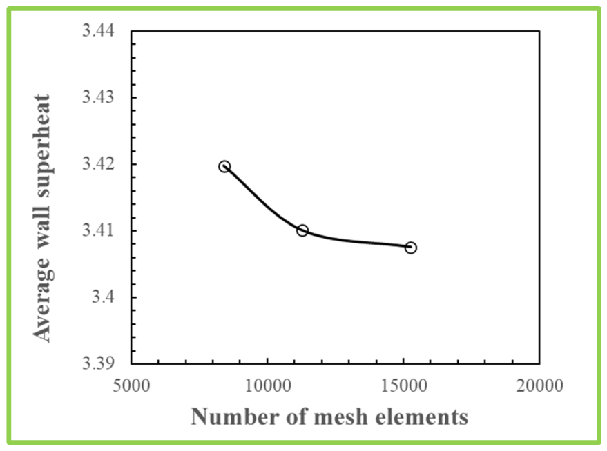
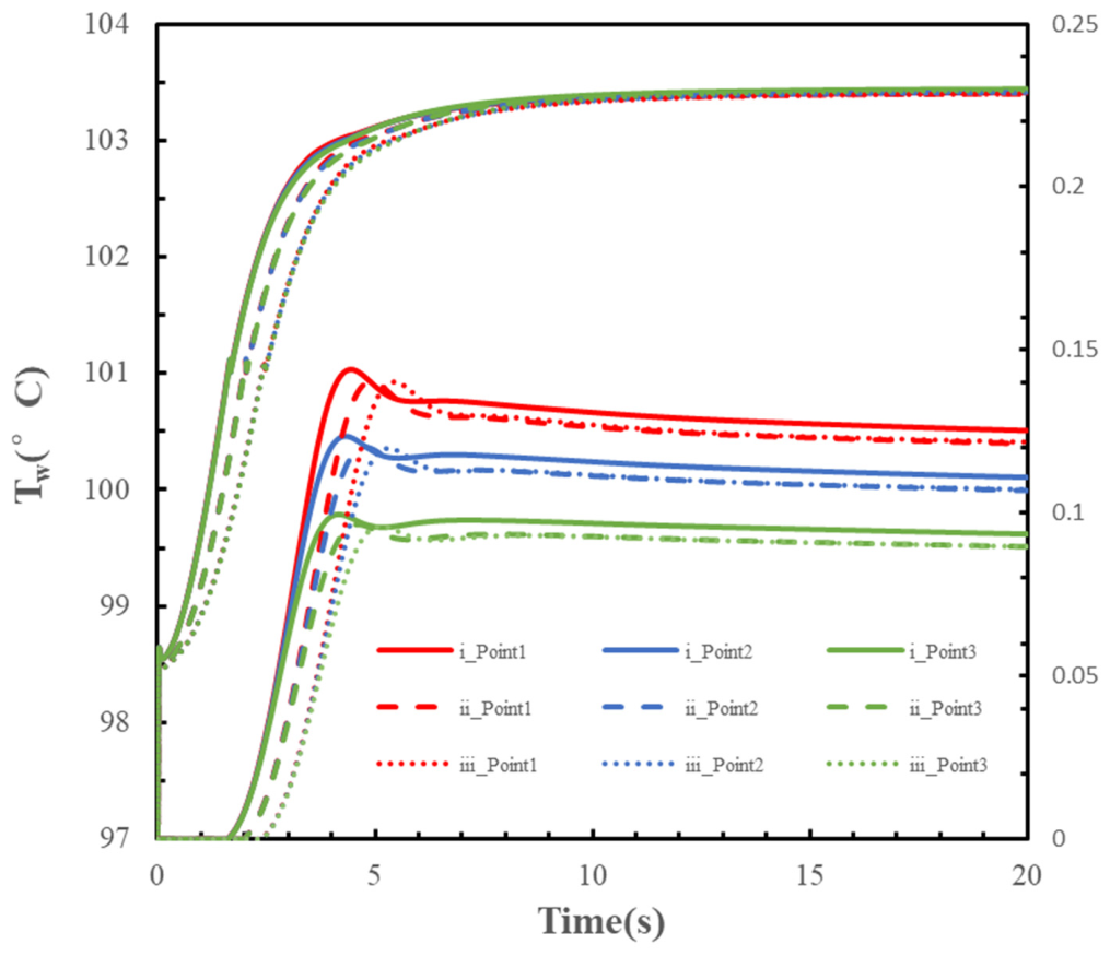
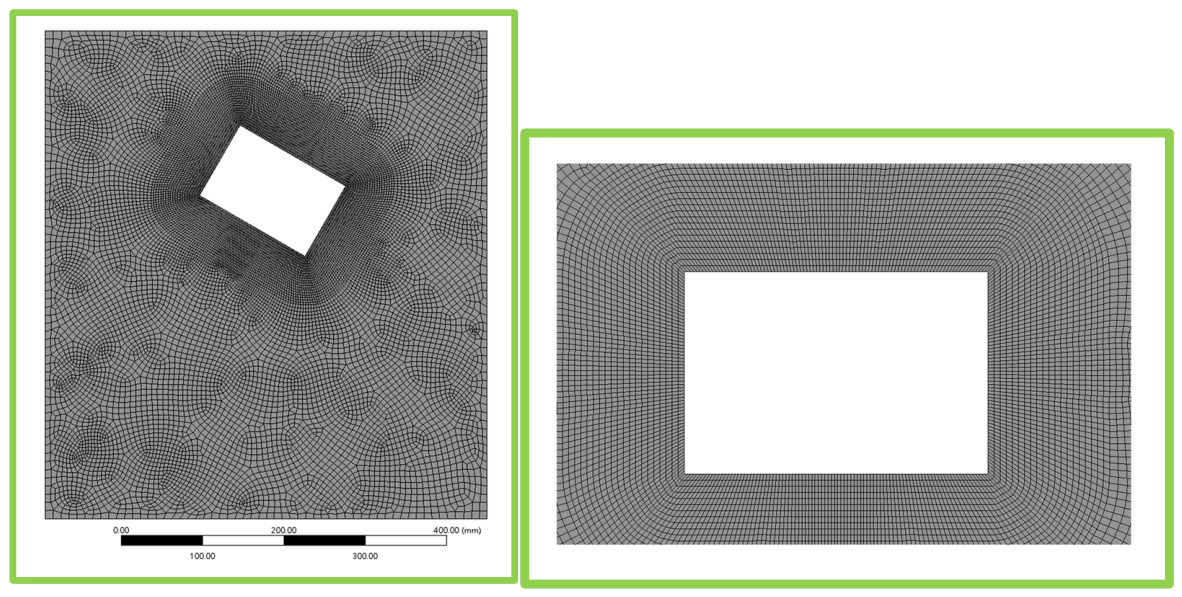
To ensure the mesh independence of the simulation results, a mesh independence study was conducted in case I, with a wall heat flux of 33,059.16 W/m2. Three different meshes were evaluated. To accurately resolve the thermal and velocity gradients within the near-wall boundary layer, 20 inflation layers were specifically applied adjacent to the heating surface across all evaluated mesh configurations. The method for adjusting the mesh properties involved increasing the mesh element number with a factor of about 1.3, while the mesh size along the wall was simultaneously reduced with a factor of 1.3. Mesh convergence was evaluated using the Grid Convergence Index (GCI) provided by The American Society of Mechanical Engineers [27]. The parameters used for calculating the GCI included the number of mesh elements and the average wall superheat at three points from 15 to 20 s. The complete parameters and the results of the mesh independence analysis are summarized in Table 2 and illustrated in Figure 2 The GCI values calculated for Mesh ii and Mesh iii show a significant decrease compared to those for Mesh i and Mesh ii, indicating that the simulation results converge when the mesh properties change from Mesh i to Mesh iii. Figure 3 shows the changes in wall temperature and void fraction over time for different mesh configurations, also indicating that Mesh iii demonstrates independence in the simulated results. Therefore, Mesh iii, as shown in Figure 4, was adopted for the downward heating simulation in this research.

2.8. Time Step Size Sensitivity Analysis

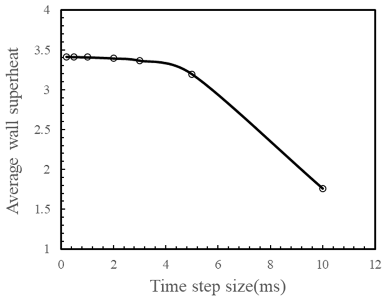
To accurately capture the highly unsteady-state boiling phenomena and ensure temporal convergence, a comprehensive time step sensitivity analysis was conducted. As suggested by the Cole correlation (Equation (27)), the frequency of bubble departure for millimeter-scale bubbles in this pool boiling scenario can reach the order of 102 to 103 1/s. Therefore, selecting an appropriately small time step size is critical to resolving these high-frequency bubble dynamics and preventing numerical distortion. The transient simulations were evaluated using seven different time step sizes: 0.2, 0.5, 1.0, 2.0, 3.0, 5.0, and 10.0 ms. The analysis was performed under the same operating conditions as those of the mesh independence study. As illustrated in Figure 5, the predicted average wall superheat exhibits a significant drop when the time step size exceeds 3.0 ms, indicating that larger time steps fail to capture the transient boiling characteristics accurately. However, as the time step decreases to 2.0 ms and below, the simulated results stabilize at approximately 3.41, demonstrating clear time step independence. Consequently, to achieve an optimal balance between computational efficiency and high numerical accuracy, a time step size of 1.0 ms was adopted for all subsequent transient calculations in this study.

3. Results and Discussion

3.1. Initial and Boundary Conditions

The simulations were performed under the initial condition of 1 atmosphere pressure and a total water temperature of 97 °C for a transient analysis over 20 s. The heating surface material was set as copper (ρ = 8978 kg/m3, Cp = 381 J/kg·K, and λ = 387.6 W/m·K). To replicate the experimental conditions and minimize heat loss [21], the other faces of the heating block were enveloped by materials modeled as ideal insulators. In the simulation, to ensure an adiabatic-like boundary and prevent heat leakage to non-fluid sides, this insulating region was assigned a practically negligible thermal conductivity (λ = 10−10 W/m·K). Owing to the essential impact of different roughnesses on the heating surface on wall temperature, the wall roughness was set to 46 μm for Sand-Grain roughness (with a roughness constant of 0.5) to match the experimental conditions. Sand-Grain roughness affects the calculated parameters of the wall function for mean velocity and viscous heating, thereby simulating the impact of roughness on heat transfer near the wall. Since the experimental conditions involved applying heat to the heating surface at constant voltages, the simulation similarly applied fixed heat fluxes to the heating surface within heat fluxes ranging from approximately 3 kW/m2 to 6 kW/m2.

3.2. Analysis of Simulated Results

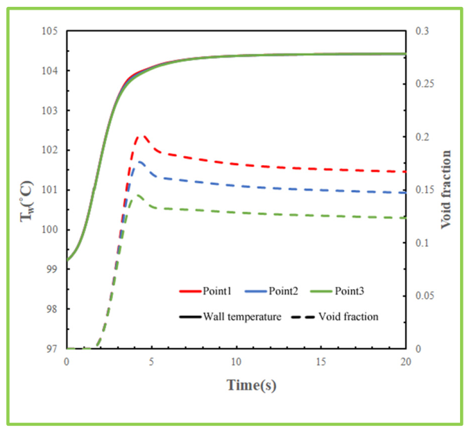
The experimental data for wall temperature and bubble dynamic parameters were averaged spatially and temporally under steady-state conditions. Therefore, it is crucial to determine whether the transient simulation data had reached the steady state when analyzing these results. Figure 6 shows the trend over time for the simulated wall temperatures and the void fractions at the three points on the heating surface, using case I with a heat flux of 51,265.91 W/m2. The wall temperatures are represented as solid lines, while the void fractions are shown as dashed lines. From 0 to 3 s, the wall temperatures increase significantly with time, and the rate of temperature increase gradually slows down from 3 to 5 s. The solid lines indicate that the wall temperatures incrementally reach a steady state after 5 s. Additionally, there are virtually no differences in wall temperature among the three points. To ensure a more rigorous verification of whether the wall temperatures had reached the steady state, we can compare the average wall temperature values over different time intervals. The time intervals are selected as 5 to 20 s, 10 to 20 s, and 15 to 20 s. From the slight differences between the average wall temperatures for three points over different time intervals, it can be determined that the 20 s transient simulation results are sufficient to be considered a steady state. Therefore, the stable simulation results can be used to analyze differences and similarities in terms of the experimental measurements.
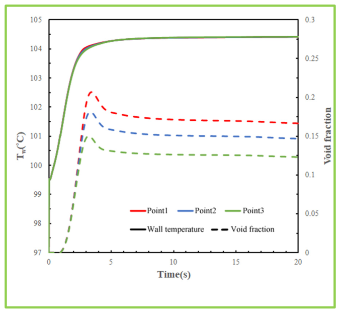
Figure 7 shows the simulation results under the same conditions as Figure 6, with the difference being that the SST k-ω turbulence model is used in the former. A comparison between the two reveals only negligible differences in the changes in both wall temperature and void fraction over different times. Additionally, under other different heat flux conditions, similar consistencies between the two turbulence models were observed. In other words, for the downward boiling heating model in this study, there is minimal difference between the standard k-ε turbulence model and the SST k-ω turbulence model in terms of their impact on calculating heat transfer and bubble behavior.
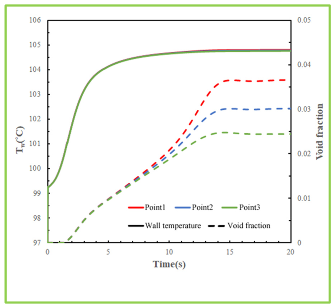
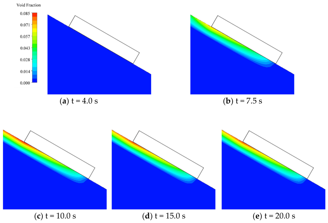
The result incorporating the Ranz–Marshall model is shown in Figure 8, which also used the simulation conditions of case I. Due to the heat transfer effects between the two-phase interface, the trend in wall temperature becomes slightly more moderate. Additionally, the predicted heat transfer capability of fluid will decrease, leading to a slight increase in wall temperature compared to when the effect is not considered. The rate at which the wall temperature reaches stability also decreases. Compared to the wall temperature, incorporating this model has a greater impact on the void fraction. The time required for the void fraction to reach stability increases, and its value decreases. The reason for this might be that the heat transfer between the phases causes the liquid temperature to rise, and it results in a decrease in the bubble departure diameter according to Equation (26). Similarly, this will affect bubble departure frequency, causing it to increase, but the impact follows a square root relationship. Therefore, the void fraction is much lower when considering the heat transfer between the phase interface.
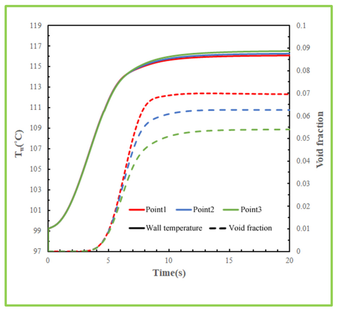
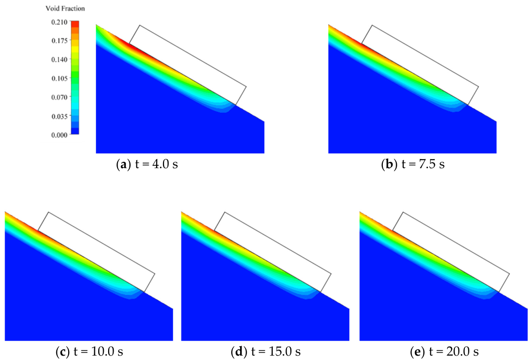
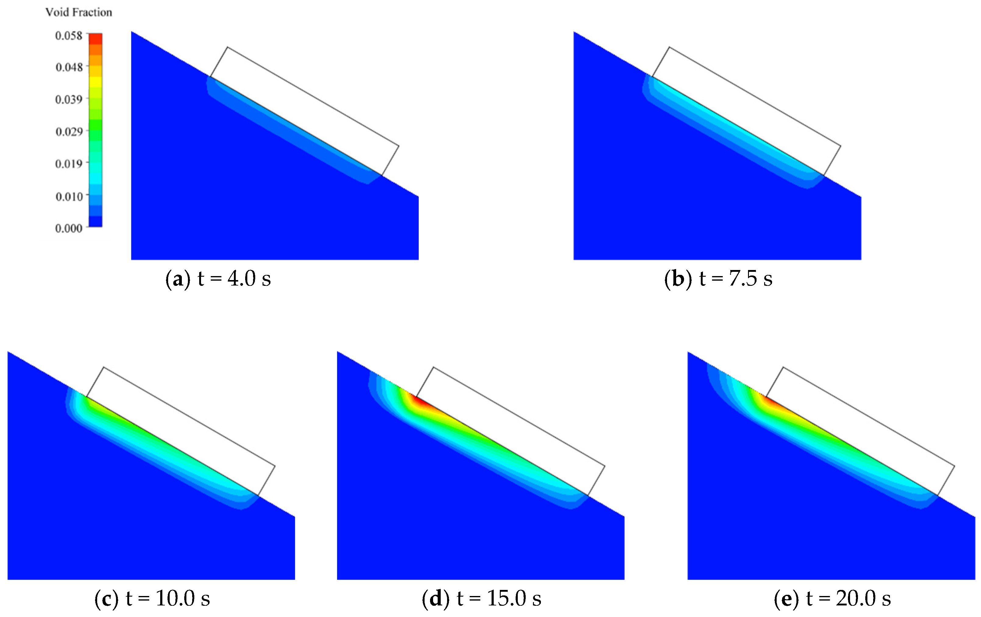
The results simulated using case II are shown in Figure 9. Compared to the results from case I, it can be concluded that the wall temperature is significantly higher, while the void fraction is lower. The trend in the increase in the void fraction is also different. When using case II, the time for the void fraction to reach a steady state is longer, and the rate of increase is more gradual. Similarly to the simulation results of the void fraction, the time required for the wall temperature to reach a steady state is also longer. The difference between case I and case II lies in the empirical formulas used for the bubble departure diameter and nucleation site density. The variation in these simulation results underscores the fact that bubble dynamic parameters have a direct impact on local boiling heat transfer. To quantitatively elucidate the underlying mechanism of these variations, the local boiling parameters and the resulting heat flux partitioning fractions at a constant heat flux for both cases are compared in Table 3. The differences in the results for the bubble departure diameter and nucleation site density calculated from case II compared to case I lead to variations in the bubble influence area. In Equations (29)–(33), these parameters directly affect the distribution of various heat fluxes, resulting in a significant difference in heat transfer efficiency between the two cases. As demonstrated in Table 3, the correlation used in case II predicts a substantial decrease in both nucleation site density and bubble departure frequency. Consequently, the evaporation heat flux fraction, which directly governs vapor generation, sharply drops from 8.43% in case I to 2.30% in case II. This suppression of evaporative heat transfer intrinsically limits the vapor generation rate, explaining the lower void fraction and its more gradual increase observed in Figure 9.
Furthermore, this shift in heat partitioning dictates the elevation in the wall temperature. In case I, the highly efficient boiling-induced heat transfer (the sum of qq and qe) accounts for 77.46% of the total heat flux. Conversely, in case II, this boiling contribution shrinks to 29.51%. To dissipate the same constant total heat flux, the system modeled by case II is forced to rely predominantly on qc, whose fraction surges from 22.54% to 70.49%. Since the single-phase convection of liquid is less efficient than phase-change heat transfer, a larger driving temperature difference between the wall and the bulk liquid is required to maintain the energy balance, inevitably leading to a significantly higher wall temperature and prolonged time to reach a steady state.

3.3. Bubble Distribution Comparison

In the heat transfer process of two-phase flow boiling, the bubble distribution is a crucial factor in local heat transfer effects. As established in the preceding sections, the transient simulations achieve steady-state conditions. The simulation conditions in Figure 10, Figure 11 and Figure 12 correspond to the heat transfer conditions in Figure 6, Figure 8 and Figure 9, respectively. They show the distribution of void fractions for the two cases at different time steps under the same heat flux. It can be observed that case I reaches a steady state after 7.5 s, while case II, although slower, also reaches a steady state after 10 s. These results are consistent with the previous conclusion.
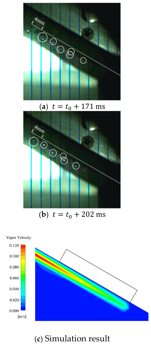
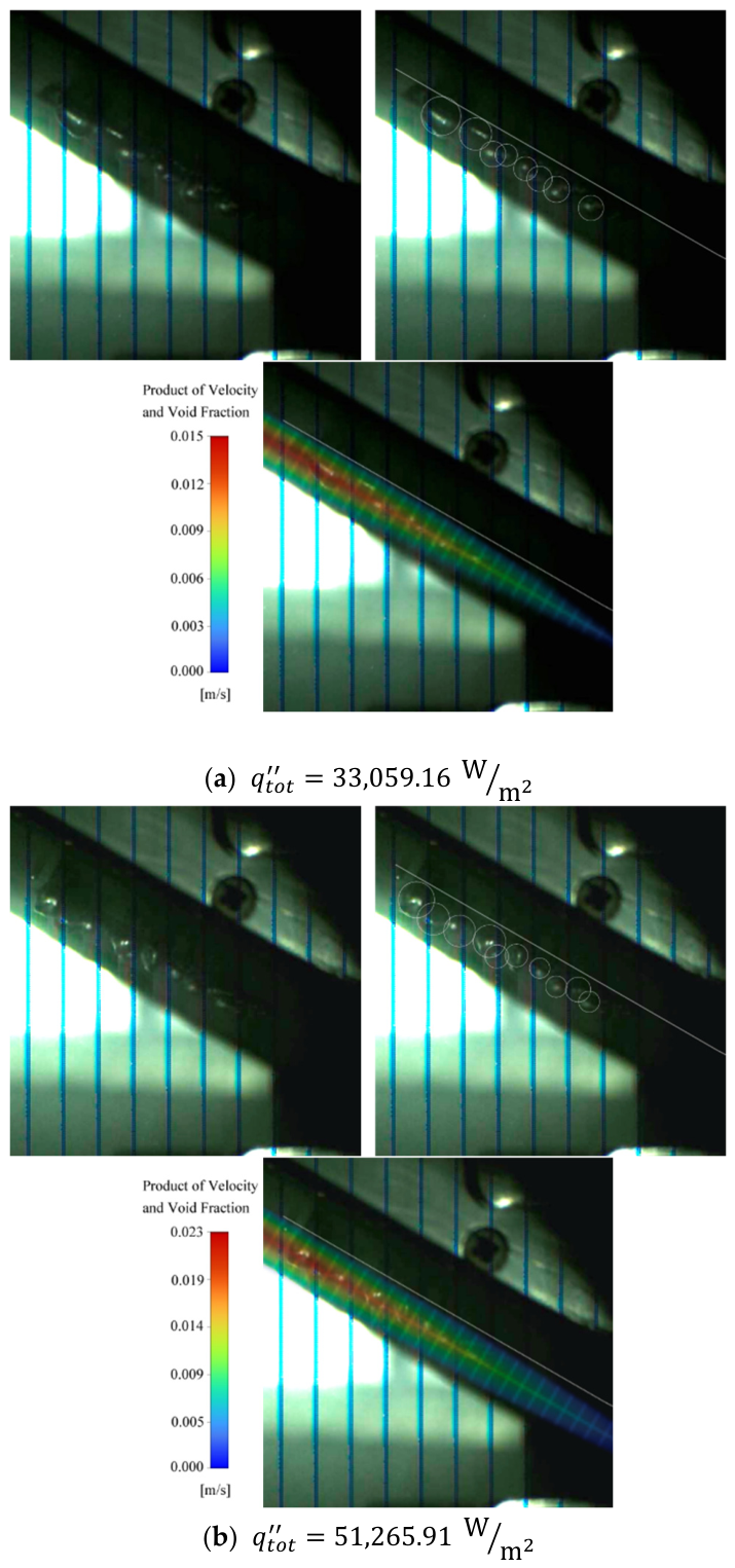
Figure 13 presents photographs of bubbles taken at different time points during the experiment. Since the simulation results are displayed using the Eulerian method, for comparison purposes, the velocities of bubbles from different experiments were averaged and simplified into a single value to be compared with the simulated vapor-phase velocity. The average experimental bubble velocity is approximately 0.105 m/s, while the simulated velocity at the same heat flux, in the middle layer from the upper to the middle sections of the heating surface, ranges from about 0.12 to 0.09 m/s. This result is close to the experimental value, with a reasonable error of up to approximately 16.7%. It should be highlighted that such a deviation is entirely acceptable and inherent to the Eulerian two-fluid framework. Because the Eulerian approach relies on the spatial and temporal averaging of multiphase flow fields, it inherently smooths out individual, sub-grid-scale discrete bubble interfacial dynamics. Predicting precise instantaneous velocities for discrete bubbles remains a classic challenge for continuum-based macroscopic models, making the current deviation well within reasonable engineering tolerances.
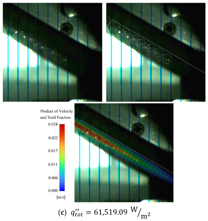
To more accurately compare the simulation results with the bubble characteristics observed in experiments, this study analyzes the bubble thickness along the heating wall surface. The product of the simulated vapor-phase velocity magnitude and the void fraction could effectively illustrate the regions where bubbles exist. Experimental bubble photos, overlaid with these simulation results under different heat fluxes, are presented in Figure 14. From the experimental photographs, it can be observed that the bubble distribution along the heating surface shows a tendency where bubbles near the upper section become larger and their thickness wider. Additionally, as the heat flux increases, the bubble distribution becomes denser, and thickness also exhibits an increasing trend. In the overlaid comparison, it can be observed that the location of the widest bubble aligns closely with the area of the highest simulated product values. Similarly, the distribution of the simulated product along the heating surface also exhibits an increasing trend upward. Moreover, as the heat flux increases, the overall value of the product rises accordingly. This indicates that the simulation under these conditions can effectively predict the bubble thickness near the heated surface. From the photographs in Figure 13b, the ratio of the bubble-occupied area to the heating surface area can be used to calculate the void fraction at this heat flux, which is approximately 0.14. Comparing to the simulated void fraction distributions, it is quite close to the results simulated by case I, and there is a larger difference from the results of case II. Although quantitative hydrodynamic validation is primarily restricted to these specific indicators, this limitation arises from the intrinsic experimental difficulties in downward-facing boiling configurations. In such geometries, the substantial accumulation and sliding of vapor bubbles beneath the heating surface severely obstruct optical paths, restricting the availability of high-resolution local velocity fields or continuous void fraction profiles. Nevertheless, the combination of the boiling curve and the key hydrodynamic parameters investigated here provides a reliable foundation to validate the model’s fidelity.
It should be noted that the present numerical study adopts a 2D computational domain. In the actual 3D downward-facing boiling phenomenon, bubbles can slide transversely, and natural convection has transverse components, allowing vapor to escape from the lateral edges. A 2D model, inherently lacking this lateral degree of freedom, traps the vapor in a single plane and forces bubble coalescence, which generally tends to overestimate the local void fraction and bubble thickness. Nevertheless, the application of a 2D approach in this study can be reasonably justified by the specific configuration of the experimental setup and the observation methodology. The dimensions of the observed heating area are 40 mm in length and 20 mm in width. Although 3D lateral effects may exist, the 20 mm width is sufficient to mitigate dominant lateral boundary constraints, allowing the 2D model to reasonably capture the primary longitudinal bubble sliding behavior. Furthermore, the experimental bubble dynamics were recorded entirely from a side-view perspective, and the extracted data represent a spatiotemporal average of the flow field. Under these conditions, the bubble distribution and the resulting void fraction can be considered to possess a quasi-two-dimensional symmetry along the transverse direction. Consequently, since the experimental void fraction is also evaluated based on the 2D projected area ratio from these side-view photographs, the comparison essentially aligns on a consistent 2D area fraction basis. Despite the inherent geometric constraints that prevent the reproduction of lateral bubble migration, the 2D approach adopted in this study, particularly in case I, successfully captures the physical trend in bubble thickness growth and provides a reasonable, slightly conservative prediction of the void fraction distribution along the main sliding direction.
For the result coupling the Ranz–Marshall model, there are significant differences in the bubble characteristics observed in the experimental setup, with a less uniform bubble distribution and much lower void fraction distribution along the heated surface. Therefore, it can be concluded that the bubble characteristics of this local downward heating boiling heat transfer achieve better simulation results without the incorporation of the Ranz–Marshall model.

3.4. Boiling Curve

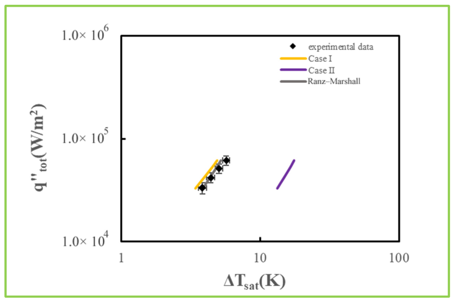
Apart from evaluating the stability of the simulation and comparing bubble characteristics with experimental observations, the boiling curve constitutes a fundamental aspect of two-phase flow heat transfer simulations. Experimental data consisted of the averages of the time and spaces measured under the constant wall heat fluxes. The measured ΔTsat showed a positive correlation with the total heat flux, and the standard deviation of the measured Tw can be evaluated by Equation (34).
E T w = ( σ k k ) 2 + ( σ x x ) 2 + ( σ q q ) 2 + ( σ T t c T ¯ t c ) 2
In Figure 15, it can be observed that the simulation results under the case I conditions are quite close to the experimental data, although the heat transfer effect exhibits a slightly higher trend. However, after incorporating the Ranz–Marshall model for interfacial heat transfer, the simulation results fall almost entirely within the experimental boiling curve’s margin of error. In contrast, the simulation results for case II show a significant deviation from the experimental values, indicating that these conditions are not suitable for the downward-facing heated surface in this boiling heat transfer study. Therefore, when considering only the predictive accuracy of heat transfer effects, the conditions of case I combined with the Ranz–Marshall model are the most suitable for this study. However, even without accounting for interfacial heat transfer, case I still demonstrates sufficient capability to effectively simulate heat transfer effects.

4. Conclusions

This paper presents a comparative analysis between CFD simulation results and experimental observations for downward-facing boiling heat transfer under various empirical correlation combinations. Through the application of the GCI method to assess grid convergence based on wall temperature, appropriate grid conditions were adopted for subsequent comparisons under different conditions. Furthermore, by analyzing the temporal changes in wall temperature and void fraction at various points, it was found that all simulation conditions reached a steady state, allowing for a comparison with experimental data. The analysis also revealed that different turbulence models had a negligible impact on the simulations in this study. Case I demonstrated reliable predictive capabilities for heat transfer effects, and its accuracy was further improved when the Ranz–Marshall model for interfacial heat transfer was incorporated. Bubble velocity, thickness, and void fraction distribution were compared with experimental images and different simulation results, indicating that case I performs well in predicting local bubble characteristics. However, after including interfacial heat transfer effects, there were significant deviations in the prediction of bubble characteristic distributions. Therefore, under the conditions of using case I and excluding the effects of interfacial heat transfer, both the heat transfer effects and bubble characteristics—two critical parameters for boiling phenomena—can be reasonably simulated and predicted for subcooled downward-facing boiling heat transfer using CFD.

Author Contributions

Y.-H.C.: Software and Analysis; Validation; Methodology; Investigation; Writing—original draft preparation. Y.-M.F.: Supervision; Project administration; Conceptualization; Methodology; Investigation; Writing—review and editing. All authors have read and agreed to the published version of the manuscript.

Funding

NSTC 114-2221-E-007-110.

Data Availability Statement

Restrictions apply to the availability of these data. Data can be made available with the permission of authors.

Acknowledgments

This work was supported by National Science and Technology Council of Taiwan under NSTC 114-2221-E-007-110.

Conflicts of Interest

The authors declare no conflicts of interest.

Nomenclature

Roman letters
Abarea fraction of bubble influence
Aiinterfacial area density (1/m)
CDdrag coefficient
CLlift coefficient
Cpspecific heat capacity (J/kg·K)
CWLwall lubrication coefficient
ddiameter
Ddbubble departure diameter
Erelative measured error
FDinterfacial drag force (N/m3)
FLinterfacial lift force (N/m3)
FTDturbulent dispersion force (N/m3)
FDwall lubrication force (N/m3)
fsbubble departure frequency (1/s)
ggravitational acceleration vector (m/s2)
hspecific enthalpy (J/kg)
hcconvective heat transfer coefficient of liquid phase (W/m2·K)
hvconvective heat transfer coefficient of vapor phase (W/m2·K)
hlvlatent heat of vaporization (J/kg)
Jasubsubcooled Jakob number
Kpqinterphase momentum exchange coefficient
Mkinterfacial momentum transfer term (N/m3)
NuNusselt number
nAnucleation site density (1/m2)
Ppressure (Pa)
Qpqvolumetric rate of energy transfer (W/m3)
q heat flux (W/m2)
ReReynolds number
Ttemperature (K)
ttime (s)
uvelocity vector (m/s)
Greek letters
αvoid fraction
Δdifference
λthermal conductivity (W/m·K)
μdynamic viscosity (Pa·s)
ρdensity (kg/m3)
σsurface tension (N/m)
τshear stress tensor (N/m2)
Subscripts
critcritical
ddeparture
lliquid phase
pdispersed phase
qcontinuous phase
rrelative
satsaturation
tturbulent
tottotal
vvapor phase
wwall

Appendix A. Sensitivity Analysis of Near-Wall Treatments
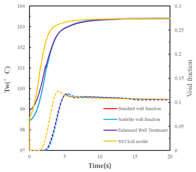
To justify the selection of the near-wall treatment, a preliminary sensitivity analysis was conducted under a representative heat flux condition of 33,509.16 W/m2. Figure A1 illustrates the transient developments of both the average wall temperature and the void fraction over 20 s using four different turbulence configurations: the standard k-ε model coupled with the standard wall function, Scalable Wall Function, and enhanced wall treatment (EWT), as well as the SST k-ω model. As shown in this figure, while the SST k-ω model exhibits a slightly faster response during the initial transient phase, all four configurations eventually converge to practically identical steady-state values for both the wall temperature and the void fraction. This explicitly verifies the numerical robustness discussed in Section 2.5, confirming that the specific near-wall treatment for single-phase convection does not compromise the macroscopic multiphase pool boiling predictions. Furthermore, regarding the near-wall mesh resolution, y+ over the heating surface for the selected Mesh iii was rigorously evaluated and found to range from approximately 8 to 26. Although these values fall outside the standard log-law region (y+ > 30) and span the transitional region approaching the viscous sublayer, the physical near-wall cell size (approximately 1.6 mm) remains larger than the empirically calculated bubble departure diameter. In the framework of the Eulerian–Eulerian multiphase flow and the RPI wall boiling model, it is fundamentally required that the control volume encompasses the dispersed phase to properly formulate the spatial phase-averaged volume fractions. Therefore, this specific mesh resolution correctly satisfies the underlying mathematical assumptions of the multiphase models applied in this study.
Figure A1. Temporal evolution of three-point averaged wall temperature and void fraction using various turbulence configurations.
Processes 14 01741 g0a1

References

  1. Huang, Y.; Wang, M.; Qiu, S.; Zhang, K.; Tian, W.; Zhang, Z. Numerical study on the thermal hydraulic characteristics of ERVC system. Ann. Nucl. Energy 2025, 211, 110972. [Google Scholar] [CrossRef]
  2. Jung, J.Y.; Lee, M.S.; Park, H.M.; Jeong, Y.H. Flow boiling experiments for CHF evaluation under downward-facing heating including flow visualization: Effects of pressure, orientation, mass flux, and local quality. Ann. Nucl. Energy 2022, 171, 108994. [Google Scholar] [CrossRef]
  3. Wang, K.; Hong, Z.; Liang, H.; Junya, I.; Cheng, S.; Okamoto, K. Experimental investigation on the characteristics of bubble growth and slide on a downward-facing heater surface in flow boiling. Int. J. Therm. Sci. 2023, 184, 108008. [Google Scholar] [CrossRef]
  4. Lee, M.S.; Yu, H.S.; Jung, J.Y.; Kam, D.H.; Jeong, Y.H. Experimental analyses of flow boiling heat transfer on downward-facing surface at low inclination: Critical heat flux and vapor bubble dynamics. Int. J. Heat Mass Transf. 2025, 244, 126960. [Google Scholar] [CrossRef]
  5. Gesmier, G.; Wang, S.; Miwa, S.; Okamoto, K. Performance evaluation of flow boiling CHF correlations in short-heated channel. Prog. Nucl. Energy 2025, 181, 105629. [Google Scholar] [CrossRef]
  6. Kurul, N.; Podowski, M.Z. Multidimensional effects in forced convection sub-cooled boiling. In Proceedings of the 9th International Heat Transfer Conference, Jerusalem, Israel, 19–24 August 1990. [Google Scholar]
  7. Han, J.; He, W.; Liu, Y.; Gao, D.; Zhao, C.; Bo, H. Numerical investigation of flow boiling characteristics in narrow rectangular channels using two-fluid Eulerian CFD model covering a wide range of pressures. Appl. Therm. Eng. 2024, 255, 123982. [Google Scholar] [CrossRef]
  8. Wang, M.; Li, L.; Liu, K.; Zhang, J.; Tian, W.; Qiu, S.; Su, G. Development of subcooled wall boiling model considering bubble sliding in narrow rectangular channel. Int. J. Therm. Sci. 2022, 181, 107787. [Google Scholar] [CrossRef]
  9. Amidu, M.A.; Addad, Y. An enhanced model for the prediction of slug flow boiling heat transfer on a downward-facing heated wall. Ann. Nucl. Energy 2020, 145, 107596. [Google Scholar] [CrossRef]
  10. Wei, L.; Pan, L.M.; Liu, H.B.; Ren, Q.Y.; He, H.; Cen, K.; Wang, D.G.; Yan, M.Y. Assessment of wall heat flux partitioning model for two-phase CFD. Nucl. Eng. Des. 2022, 390, 111693. [Google Scholar] [CrossRef]
  11. Ranz, W.E.; Marshall, W.R., Jr. Evaporation from drops, Part I. Chem. Eng. Prog. 1952, 48, 141–146. [Google Scholar]
  12. Ranz, W.E.; Marshall, W.R., Jr. Evaporation from drops, Part II. Chem. Eng. Prog. 1952, 48, 173–180. [Google Scholar]
  13. Yang, S.; Ren, B.; Yang, L.; Chen, C.; Lu, Q.; Wei, Z. Investigation of the impact of near-wall mesh size on the transition from microscopic wall boiling mechanism to macroscopic multiphase-CFD models. Appl. Therm. Eng. 2024, 244, 122678. [Google Scholar] [CrossRef]
  14. Ishii, M. Two-fluid model for two-phase flow. In Proceedings of the 2nd International Workshop on Two-Phase Flow Fundamentals, Troy, NY, USA, 1 October 1979. [Google Scholar]
  15. Drew, D.A.; Lahey, R.T. The virtual mass and lift force on a sphere in rotating and straining inviscid flow. Int. J. Multiph. Flow 1987, 13, 113–121. [Google Scholar] [CrossRef]
  16. Moraga, F.J.; Bonetto, F.J.; Lahey, R.T. Lateral forces on spheres in turbulent uniform shear flow. Int. J. Multiph. Flow 1999, 25, 1321–1372. [Google Scholar] [CrossRef]
  17. Antal, S.P.; Lahey, R.T., Jr.; Flaherty, J.E. Analysis of phase distribution and turbulence in dispersed particle/liquid flows. Chem. Eng. Commun. 1991, 174, 85–113. [Google Scholar]
  18. Burns, A.D.; Frank, T.; Hamill, I.; Shi, J.M. The Favre averaged drag model for turbulent dispersion in Eulerian multi-phase flows. In Proceedings of the 5th International Conference on Multiphase Flow, Yokohama, Japan, 30 May–4 June 2004. [Google Scholar]
  19. Lavieville, J.; Quemerais, E.; Mimouni, S.; Boucker, M.; Mechitoua, N. NEPTUNE CFD V1.0 Theory Manual; EDF: Paris, France, 2005. [Google Scholar]
  20. Del Valle, V.H.; Kenning, D.B.R. Subcooled flow boiling at high heat flux. Int. J. Heat Mass Transf. 1985, 28, 1907–1920. [Google Scholar] [CrossRef]
  21. Tseng, Y.L.; Ferng, Y.M. Experimental investigation of pool boiling heat transfer and bubble dynamics for the downward facing heating. Ann. Nucl. Energy 2022, 174, 109198. [Google Scholar] [CrossRef]
  22. Tolubinski, V.I.; Kostanchuk, D.M. Vapor bubbles growth rate and heat transfer intensity at subcooled water boiling. In Proceedings of the 4th International Heat Transfer Conference, Paris, France, 31 August–5 September 1970. [Google Scholar]
  23. Lemmert, M.; Chawla, L.M. Influence of flow velocity on surface boiling heat transfer coefficient. In Heat Transfer in Boiling; Hahne, E., Grigull, U., Eds.; Academic Press and Hemisphere: New York, NY, USA, 1977. [Google Scholar]
  24. Cole, R. A photographic study of pool boiling in the region of the critical heat flux. AIChE J. 1960, 6, 533–542. [Google Scholar] [CrossRef]
  25. Kocamustafaogullari, G.; Ishii, M. Interfacial area and nucleation site density in boiling systems. Int. J. Heat Mass Transf. 1983, 26, 1377–1387. [Google Scholar] [CrossRef]
  26. Kocamustafaogullari, G.; Ishii, M. Foundation of the interfacial area transport equation and its closure relations. Int. J. Heat Mass Transf. 1995, 38, 481–493. [Google Scholar] [CrossRef]
  27. ASME V&V 20-2009; Standard for Verification and Validation in Computational Fluid Dynamics and Heat Transfer. American Society of Mechanical Engineers: New York, NY, USA, 2009.
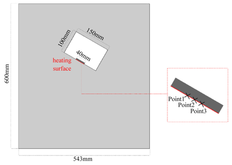
Figure 1. Schematic of two-dimensional computational geometry.
Processes 14 01741 g001
Figure 2. GCI analysis for mesh independence.
Processes 14 01741 g002
Figure 3. Transient comparison of wall temperature and void fraction at different points for various mesh models.
Processes 14 01741 g003
Figure 4. Schematic of computational mesh structure.
Processes 14 01741 g004
Figure 5. Sensitivity analysis for time step independence.
Processes 14 01741 g005
Figure 6. Transient evaluation of wall temperature and void fraction for case I.
Processes 14 01741 g006
Figure 7. Transient evaluation of wall temperature and void fraction using SST k-ω turbulence model.
Processes 14 01741 g007
Figure 8. Transient evaluation of wall temperature and void fraction coupled with Ranz–Marshall interfacial heat transfer model.
Processes 14 01741 g008
Figure 9. Transient evaluation of wall temperature and void fraction for case II.
Processes 14 01741 g009
Figure 10. Spatial distributions of void fraction at various temporal stages for case I.
Processes 14 01741 g010
Figure 11. Spatial distributions of void fraction at various temporal stages for case II.
Processes 14 01741 g011
Figure 12. Spatial distributions of void fraction at various temporal stages coupled with Ranz–Marshall model.
Processes 14 01741 g012
Figure 13. Comparison between experimental bubble morphologies and simulated steady-state vapor velocity distribution. The open circles indicate the bubble locations on the heated surface.
Processes 14 01741 g013
Figure 14. Comparison of experimental bubble layer thickness and simulated void fraction–velocity product for case I. The open circles indicate the bubble locations on the heated surface.
Processes 14 01741 g014aProcesses 14 01741 g014b
Figure 15. Comparison of experimental and simulated boiling curves under different modeling conditions.
Processes 14 01741 g015
Table 1. Summary of empirical correlations and sub-models for simulated variants.
Simulation
Variant
Turbulence Model and Near-Wall TreatmentBubble Dynamic CorrelationsInterfacial Heat Transfer
case I
(base model)
standard k-ε with
standard wall function
Dd: Tolubinsky & Kostanchu
fs: Cole
nA: Lemmert & Chawla
None
case IIstandard k-ε with standard wall functionDd: Kocamustafaogullari & Ishii
fs: Cole
nA: Kocamustafaogullari & Ishii
None
case I
with SST k-ω
SST k-ωsame as case INone
case I
with Ranz–Marshall
standard k-ε with standard wall functionsame as case IRanz–Marshall
sensitivity test
(Appendix A)
standard k-ε with
scalable wall function/enhanced wall treatment
same as case INone
Table 2. Parameter and results of mesh independence analysis based on GCI.
Number of Mesh ElementsMesh Size Along Heating Wall (mm)Average ΔTw
(K)
GCI (%)
i84042.863.4198
ii11,2802.003.41011.03
iii15,2541.603.40760.26
Table 3. Comparison of surface-averaged boiling parameters and heat flux partitioning between case I and case II at constant heat flux of 51,265.91 W/m2.
CaseDdfsnAqe
(%)
qq
(%)
qc
(%)
qv
(%)
I0.000571151.2229,374.28.4369.0322.543.25 × 10−8
II0.0046153.2106,497.82.3027.2170.496.67 × 10−9
Disclaimer/Publisher’s Note: The statements, opinions and data contained in all publications are solely those of the individual author(s) and contributor(s) and not of MDPI and/or the editor(s). MDPI and/or the editor(s) disclaim responsibility for any injury to people or property resulting from any ideas, methods, instructions or products referred to in the content.