A Method for Predicting Three Formation Pressures in Ultra-Deep Wells in the Southern Margin Based on Well–Seismic Data Fusion and Machine Learning

Abstract

Aiming at the challenges faced by ultra-deep wells in the southern margin of the Junggar Basin, such as strong uncertainty in formation information, difficulties in accurate prediction of three formation pressures, narrow safe density windows, and prominent downhole risks, this paper establishes a method for predicting three formation pressures with confidence levels and quantitatively evaluating drilling risks based on well–seismic fused data. Firstly, rock mechanics and in situ stress calculation models are optimized to characterize the strong uncertainty of deep formations. Then, high-precision well–seismic fused interval velocity is generated through multi-source data preprocessing, well–seismic data fusion, and construction of the MLP-TFT-MCMC hybrid model. On this basis, three formation pressures are calculated, and a pressure profile with confidence levels is constructed using an improved t-distribution. Verified by a field well case, the predicted results are consistent with actual data, providing technical support for the safe and efficient drilling of subsequent ultra-deep wells.

1. Introduction

With the deepening of oil and gas field exploration, oil and gas development at home and abroad has gradually expanded greatly, and the southern margin of Xinjiang’s Junggar region, located in front of the Tianshan Mountains and Bogda Mountains, is rich in oil and gas resources and has become an important strategic successor area for oil and gas development in the Junggar Basin [1]. However, the geological conditions in this area are extremely complex, and the drilling process faces the world-renowned problems of “one deep, one steep, one narrow, two thick, and three high”, leading to frequent downhole complexities and great difficulties in casing program design. How to quantitatively describe the uncertainty of deep complex formation information and conduct quantitative evaluation of potential risks before drilling is an urgent technical problem to be solved in this area, and accurate prediction of three formation pressures is the key [2,3,4].

Research on formation pressure prediction began in 1965. Initially, methods for predicting high-pressure formations based on shale resistivity and acoustic waves were developed and later evolved into a composite model that combines the Tau method and the Fillippone method for prediction based on 3D seismic data. The basic principle of these traditional methods is established on the normal compaction trend line derived from the effective stress principle: as the burial depth increases, the normal compaction trend line increases linearly and deviates when encountering abnormal pressure [5]. The main methods include the equivalent depth method, the Eaton method, the Bowers method, the Fillippone method, etc. [6,7,8]. These methods rely heavily on calibrated empirical coefficients and are mostly valid for single pressure-generation mechanisms such as undercompaction. They lack adaptability to deeply buried heterogeneous formations with coupled pressure-generation mechanisms, leading to large prediction errors and poor generalization in ultra-deep well scenarios [9,10].

In recent years, the rapid development of machine learning has provided new ideas for formation pressure prediction. For example, Yang Jin et al. [11] introduced a BP neural network to predict formation pressure based on seismic interval velocity; Keshavarzi and Jahan Bakhshi [12] applied backpropagation neural networks (BPNNs) and generalized regression neural networks (GRNNs) to accurately predict the pressure gradient of the Asmara Oilfield in Iran by inputting depth, permeability, rock density, and porosity; the Ahmed team [13] established two pore pressure gradient prediction models based on SVM and FN algorithms; Song Xianzhi et al. [14], considering that both drilling and formation deposition are sequential problems, proposed a method combining long short-term memory neural networks (LSTMs) and error backpropagation neural networks (BP) to predict formation pore pressure. However, existing machine learning models for formation pressure prediction are typically constructed using single-source or partial data as input, failing to fully exploit the complementary advantages of drilling, logging, mud logging, and seismic data. Meanwhile, the black-box nature of most machine learning models results in insufficient interpretability, which restricts their practical application and promotion in field engineering, such that these methods still need to be improved in terms of model interpretability and generalization ability, especially facing great challenges in new exploration areas where drilling data from existing wells are scarce.

Well–seismic data fusion technology and real-time updating technology for three formation pressures while drilling are key technologies to improve the accuracy of formation pressure prediction for wells to be drilled and ensure drilling engineering safety, and they have become research hotspots in the field of three formation pressure prediction in recent years. Early well–seismic data fusion technology was mainly used in geological exploration, focusing on basic geological research such as well–seismic calibration, reservoir identification, and fracture and fault discrimination. Yu Wenwen et al. [15] used the MLP deep learning algorithm to reconstruct acoustic time difference curves, effectively compensating for missing or distorted acoustic time difference data in some intervals, greatly improving the calibration effect of well–seismic integration, deepening the comprehensive geological research understanding based on well–seismic data, and providing more accurate basic data for subsequent formation pressure prediction.

Statistics play an important role in drilling geomechanics. Guan Zhichuan et al. [16,17] proposed a formation pressure prediction method with confidence levels, which quantitatively characterizes the uncertainty of formation information using confidence levels based on statistics of the distribution law of drilling geomechanical parameters in each formation, with strong interpretability, which is expected to solve the problem of quantitative evaluation of drilling risks in ultra-deep wells in the southern margin.

Conventional formation pressure prediction mostly relies on single logging or seismic data, suffering from insufficient vertical resolution, poor lateral representativeness, and an inability to quantify uncertainty. Although the formation pressure method with confidence levels can characterize formation uncertainty through probability statistics, traditional methods do not integrate well–seismic data and have insufficient prediction accuracy in small-sample, strongly heterogeneous formations. Therefore, this paper introduces well–seismic fusion technology and constructs a three formation pressure prediction method with confidence levels based on the MLP-TFT-MCMC hybrid model. The key research gap addressed herein is that conventional formation pressure prediction methods rely on single-source data, deterministic modeling, and fixed distribution assumptions which fail to quantify uncertainty or adapt to ultra-deep heterogeneous formations with strong heterogeneity, limited measured data, and complex pressure-generation mechanisms. Compared with traditional machine learning methods, the proposed framework avoids the black-box limitation of pure data-driven models and integrates physical prior knowledge; compared with deterministic statistical methods, it provides confidence intervals and uncertainty quantification. These improvements fill the gap of reliable pre-drilling pressure prediction under small-sample, strong-heterogeneity conditions in southern margin ultra-deep wells.

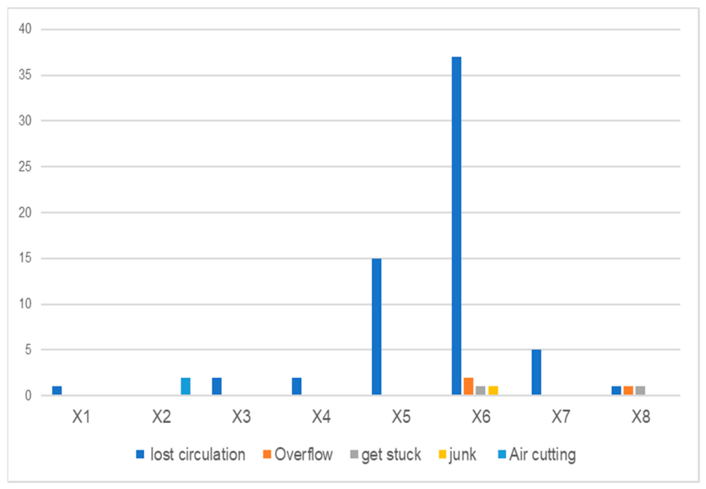
Statistics of downhole complexities in eight wells drilled in this area show that risks occur in almost every well, especially Well X6, which has the highest frequency. The most frequent downhole complexity is lost circulation, accounting for 89%. According to statistics by formation, complexities mostly occur in low-pressure-bearing formations of the Donggou Formation, high-pressure formations of the Qingshuihe Formation, low-pressure-bearing glutenite formations of the Kalazha Formation, and interbedded mudstone and sandstone of the Qigu Formation (Figure 1).

Figure 1. Statistics of complex situations in the southern margin area.

2. Methods

2.1. Existing Calculation Method for Three Formation Pressures with Confidence Levels

To address the difficulty in accurately predicting the three pressures (pore pressure, collapse pressure, and fracture pressure) of formations, the calculation of rock mechanical parameters, which mainly include elastic parameters and strength parameters, is particularly critical.

A uniform sign convention of positive for compression and negative for tension is adopted throughout this paper [18,19,20,21]. To simplify the mathematical model and facilitate subsequent quantitative and qualitative analysis of wellbore stresses, the following assumptions are specially made:

• The reservoir rock is treated as an isotropic medium.
• Stress disturbances caused by physicochemical reactions during fluid seepage are not considered.
• The rock is assumed to be a linearly elastic medium, and plastic deformation or irreversible deformation is not involved in the analysis.
• These assumptions can effectively reduce the complexity of stress calculation while ensuring the accuracy of core analysis, providing fundamental support for in-depth research in subsequent sections.

However, these assumptions have evident limitations in ultra-deep heterogeneous formations. Under high pressure, high temperature, and complex mineral composition, real formation rocks usually show anisotropy and inelastic behavior, which may cause prediction bias. In the following sections, sensitivity analysis and uncertainty quantification are used to evaluate the influence of anisotropy, and future research will further relax the assumptions of elasticity and isotropy by introducing anisotropic mechanical models [22,23,24,25,26].

Elastic parameters mainly characterize the deformation characteristics of rocks, including Young’s modulus and Poisson’s ratio, which can be divided into dynamic and static types. Static elastic parameters are generally measured through laboratory core tests, while dynamic elastic parameters are calculated based on acoustic interval transit time. Therefore, static elastic parameters can better reflect the real characteristics of rocks. However, in practical engineering, it is impossible to conduct tests on rocks at every depth, so it is necessary to convert dynamic elastic parameters into static ones.

Strength parameters of rocks mainly reflect the ultimate stress at which rocks are damaged, including uniaxial compressive strength and uniaxial tensile strength. Statistics show that the calculation models of rock mechanical parameters applicable to the southern margin area are shown in Table 1 [27,28].

Table 1. Rock mechanics parameter calculation model applicable to the southern margin area.

Rock Mechanics Parameters	Computational Model
Dynamic Young’s modulus	$E_d={\displaystyle \frac{\mathsf{\rho }{V_s}^2\left(3V_p^2-4V_s^2\right)}{V_p^2-V_s^2}}\times {10}^3$
Dynamic Poisson’s ratio	${\mu }_d={\displaystyle \frac{V_p^2-2V_s^2}{2\left(V_p^2-V_s^2\right)}}$
Conversion of dynamic and static elastic parameters	${\mathsf{\mu }}_s=A_1+K_1{\mathsf{\mu }}_d;E_s=A_2+K_2{E}_d$
Uniaxial compressive strength	$S_c=0.033{\rho }^2{V}_p^4{\displaystyle \frac{{\left(1+{\mathsf{\mu }}_d\right)}^2}{\left(1-{\mathsf{\mu }}_d\right)}}\left(1-2{\mathsf{\mu }}_d\right)\left(1+0.78V_{sh}\right)$
Uniaxial tensile strength	$S_t={\displaystyle \frac{S_c}{K}}$
Cohesion	$C=0.00544{\rho }^2{V}_p^4{\left({\displaystyle \frac{1+{\mu }_d}{1-{\mu }_d}}\right)}^2\left(1-2{\mu }_d\right)\left(1+0.78V_{\mathrm{sh}}\right)$
Internal friction angle	$\varphi =\arcsin \left(\left(V_p-1\right)/\left(V_p+1\right)\right)$

Note: $V_p$ is the longitudinal wave velocity, $\mathrm{k}\mathrm{m}/\mathrm{s}$; $V_s$. is the shear wave velocity, $\mathrm{k}\mathrm{m}/\mathrm{s}$; $E_d$ is the dynamic Young’s modulus, $\mathrm{M}\mathrm{P}\mathrm{a}$; ${\mu }_d$ is the dynamic Poisson’s ratio, no factor; $\rho$ is the density of the formation body, $\mathrm{g}/\mathrm{c}{\mathrm{m}}^3$; $E_s$ is the static Young’s modulus, MPa; ${\mu }_s$ is the static Poisson’s ratio, factorless; $S_c$ is the uniaxial compressive strength, $\mathrm{M}\mathrm{P}\mathrm{a}$; $S_t$ is the uniaxial tensile strength, $\mathrm{M}\mathrm{P}\mathrm{a}$; $V_{sh}$ is the muddy content, 0~1, no factor.

Changes in in situ stress can be used as an important indicator to identify abnormal formation pressure. In situ stress has a significant impact on rock skeleton stress and pore fluid properties and is a key factor to be considered in formation pressure prediction. Regarding the calculation of in situ stress, previous studies have established sufficient calculation models, such as the Huang Rongzun model, the Ge-style model, and the combined spring model, which have achieved good results in practical working conditions [29,30].

In situ stress mainly includes vertical in situ stress and horizontal in situ stress. Vertical in situ stress is calculated by the summation method, and horizontal in situ stress is calculated using Huang’s model. The models are shown in Table 2.

Table 2. Stress calculation model applicable to the southern margin region.

Ground Stress	Computational Model
Vertical stress	$G_0={\rho }_0+A{H}^B$
Horizontal stress	$\left\{\begin{array}{c}{\sigma }_H=({\displaystyle \frac{\mu }{1-\mu }}+{\gamma }_1)\left({\sigma }_v-\alpha P_p\right)+\alpha P_p\\ {\sigma }_h=({\displaystyle \frac{\mu }{1-\mu }}+{\gamma }_2)\left({\sigma }_v-\alpha P_p\right)+\alpha P_p\end{array}\right.$

Notes: All in situ stresses are expressed in terms of relative drilling fluid density. $G_0$ is the vertical in situ stress (overburden pressure), $\mathrm{g}/\mathrm{c}{\mathrm{m}}^3$; ${\rho }_0$ is the formation density at the upper mud surface, $\mathrm{g}/\mathrm{c}{\mathrm{m}}^3$; $H$ is the well depth below the upper mud surface, $\mathrm{m}$; ${\sigma }_H$ is the maximum horizontal in situ stress, $\mathrm{g}/\mathrm{c}{\mathrm{m}}^3$; ${\sigma }_h$ is the minimum horizontal in situ stress, $\mathrm{g}/\mathrm{c}{\mathrm{m}}^3$; $\mu$ is the static Poisson’s ratio, dimensionless; ${\sigma }_v$ is the vertical in situ stress, $\mathrm{g}/\mathrm{c}{\mathrm{m}}^3$; $\alpha$ is the effective stress coefficient, dimensionless; ${\gamma }_1 \mathrm{and}{ \gamma }_2$ are tectonic stress coefficients, dimensionless.

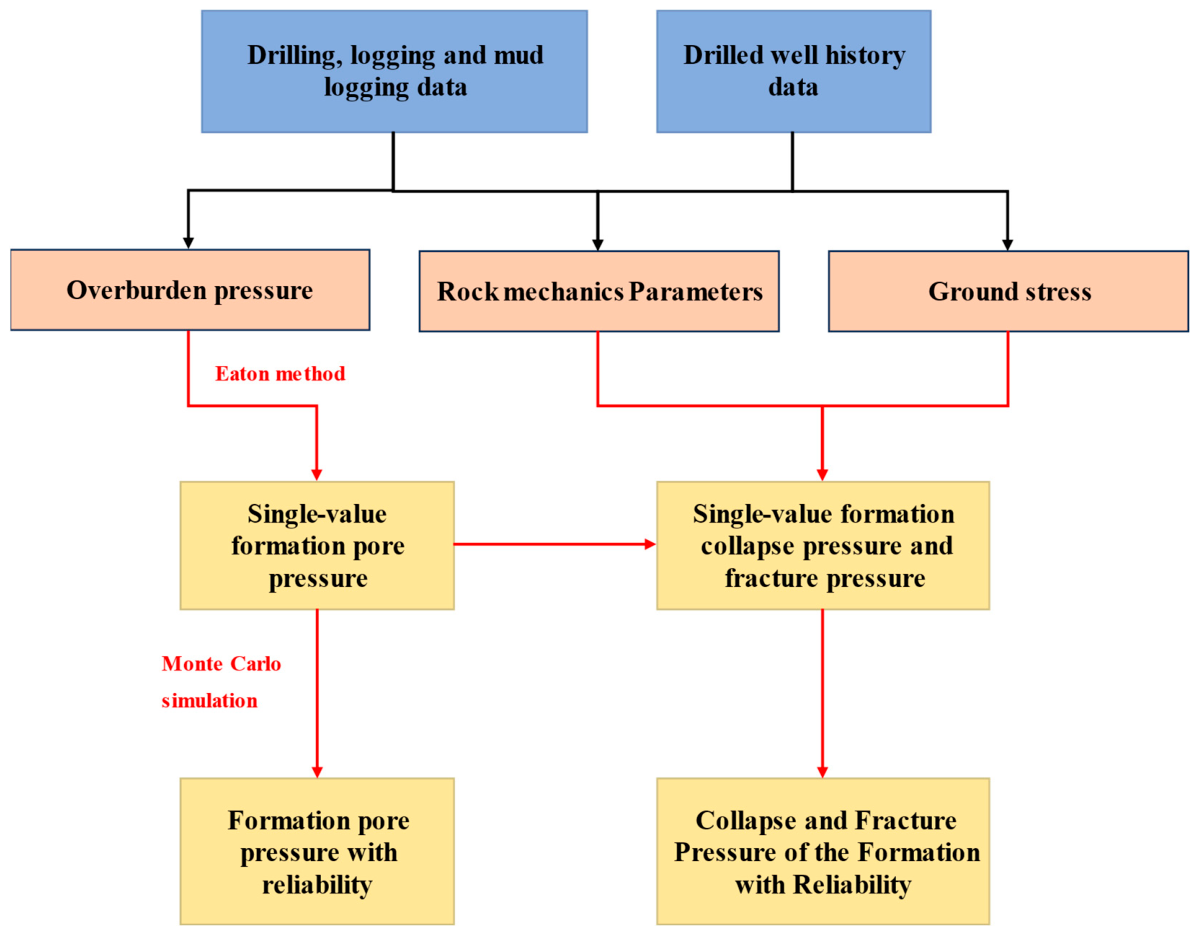
Through analysis of the subsequent outcomes, the K₂d, J₃q, and other formations have significant uncertainty. Single-value formation tri-pressure (pore pressure, collapse pressure, and fracture pressure) can no longer accurately characterize the characteristics of these formations. Therefore, this paper introduces a formation pressure prediction method with confidence levels. Taking the pore pressure with confidence levels as an example: first, the overburden pressure is calculated using the logging data, mud logging data, and well history data of existing wells in the region; then, the single-value formation pore pressure is obtained using the Eaton method; finally, the pore pressure with confidence levels is derived through Monte Carlo simulation. Taking the fracture pressure with confidence levels as an example: first, the maximum and minimum in situ stress, Poisson’s ratio, and uniaxial tensile strength are calculated using logging data, mud logging data, and well history data of existing wells in the region; then, the single-value formation fracture pressure is obtained in combination with the single-value pore pressure; finally, the fracture pressure with confidence levels is derived through Monte Carlo simulation. The calculation process is shown in Figure 2 [31,32,33].

Figure 2. Method for calculating formation tri-pressure with confidence levels.

2.2. Improved Method Based on Well–Seismic Fusion Data and T-Distributions

However, traditional formation tri-pressure calculation methods often rely on a single type of data for pressure prediction, and such single-source data cannot provide a comprehensive understanding of formation information. In this paper, we reasonably integrate seismic data, logging data, and other information, and use the high vertical resolution of logging curves to enhance the features of seismic data, which imposes more comprehensive macroscopic constraints, thereby further improving the prediction accuracy of formation tri-pressure. Furthermore, machine learning methods can effectively handle the heterogeneity between seismic and logging data, accurately capture the nonlinear relationship between them, and autonomously learn the inherent features and correlation rules of the two types of data. This breaks through the limitations of the linear assumptions in traditional methods, realizes the deep fusion of heterogeneous data, and further improves the accuracy and reliability of the fused data.

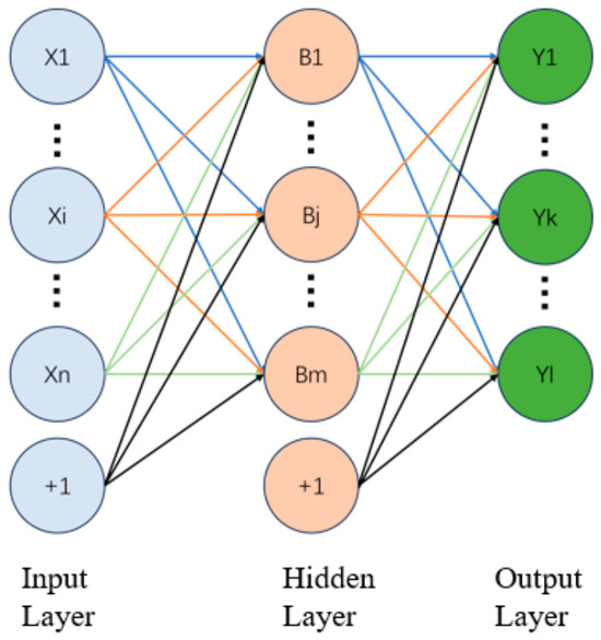
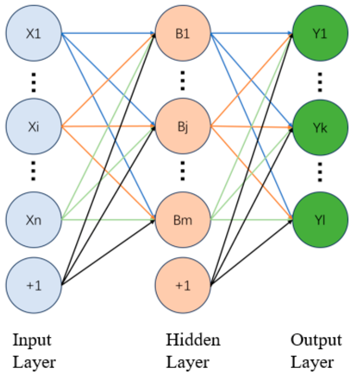
This paper focuses on adopting the MLP-TFT-MCMC hybrid model to fuse well and seismic data, giving full play to its strong capabilities in feature extraction and nonlinear fitting. The Multilayer Perceptron (MLP) consists of multiple layers of neurons, where each neuron is connected to those in the preceding and succeeding layers via weights. It mainly comprises three components: the input layer receives screened multi-source feature parameters; the hidden layer performs feature extraction on heterogeneous data through activation functions, effectively capturing the continuity of seismic data and the accuracy of logging data; finally, the output layer generates pre-drilling well–seismic fused data through dynamic weighting and biasing.

The pre-drilling well–seismic fused data, $F\left(x\right)$, is expressed as follows:

$$F(x)=G\left(b_2+W_2^T\left(f(b_1+W_1^{T}x)\right)\right)$$

where $x$ denotes the input layer, and the output of the hidden layer can be expressed as $\mathrm{f}\left({\mathrm{b}}_1+{{\mathrm{W}}_1}^{\mathrm{T}}\mathrm{x}\right)$; ${\mathrm{W}}_1$ and ${\mathrm{W}}_2$ represent the weights of the MLP model; and ${\mathrm{b}}_1$ and ${\mathrm{b}}_2$ denote the biases of the MLP model. The functions $f$ and G are sigmoid functions. A schematic diagram of the MLP model structure is shown in Figure 3.

Figure 3. Schematic diagram of MLP model structure.

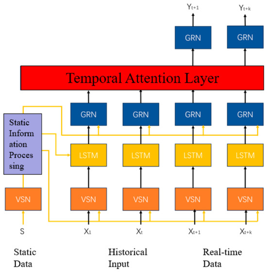
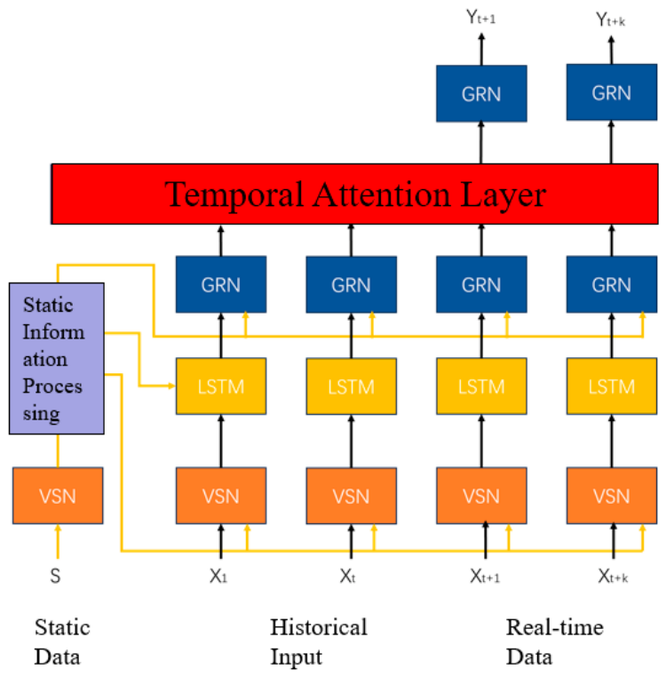
The Temporal Fusion Transformer (TFT) model is a deep learning model specially designed for time-series prediction. It integrates structures such as a Gated Residual Network (GRN), an attention mechanism, and residual connection, enabling it to capture long-term and short-term temporal dependencies, process multivariate time-series data, and quantify feature importance. This makes it well suited to the time-series characteristics of real-time updating of logging-while-drilling (LWD) data. First, the input layer hierarchically separates input data into temporal dynamic features and static features. A Variable Selection Network (VSN) assigns weights based on real-time data input at each time step.

$${\alpha }_t=\mathrm{Softmax}\left(W_v{h}_t+b_v\right)$$

Next is the core of the TFT: the Gated Residual Network (GRN), which mainly consists of a Gated Recurrent Unit (GRU) layer and a residual connection layer. As the core of the TFT for temporal feature extraction, the GRU replaces the traditional RNN structure and specifically addresses the vanishing gradient problem in long-sequence training of logging-while-drilling data.

$$z_t=\sigma (W_z{x}_t+U_z{h}_{t-1}+b_z); r_t=\sigma (W_r{x}_t+U_r{h}_{t-1}+b_r);$$

$${\tilde{h}}_t=\mathit{tanh}(W_h{x}_t+U_h(r_t\odot h_{t-1})+b_h)$$

The Gated Linear Unit (GLU) works together with the residual connection layer to ensure the stability of deep model training and the integrity of feature extraction, meeting the real-time updating requirements for complex formations. The temporal attention mechanism layer is designed for the real-time updating of well–seismic fused data, whose key function is to dynamically assign weights to data at different well depths. Finally, the feature fusion layer adapts to multi-source heterogeneous well–seismic data, integrating static features and temporal dynamic features to overcome the limitations of using single-type time-series data alone. A schematic diagram of the model structure is shown in Figure 4.

Figure 4. Schematic diagram of the TFT model structure.

Deterministic predictions from the MLP-TFT cannot reflect randomness, parameter uncertainty, or data noise, which are critical for safe drilling in ultra-deep formations. Therefore, probabilistic modeling is necessary to quantify uncertainty and provide confidence intervals. The MCMC method is introduced to realize posterior inference, uncertainty estimation, and closed-loop optimization of the TFT model, forming a complete probabilistic prediction system. Finally, the adopted Markov Chain Monte Carlo (MCMC) model, based on Markov chain theory and the Monte Carlo random sampling method, plays a core role in the MLP-TFT-MCMC hybrid model: it predicts the optimal forward exploration range and feedback-adjusts the parameters of the TFT model, forming a closed-loop regulation mechanism of TFT time-series processing–MCMC forward exploration and feedback–TFT parameter optimization, which adapts to the dynamic and forward-looking requirements of real-time updating of well–seismic fused data while drilling.

The specific mechanism and implementation steps are as follows:

(1)

Dynamic prior distribution setting: A dynamic weak-information prior distribution is constructed using real-time logging-while-drilling data and lithological rules. The state transition matrix of the Markov chain is given as follows, where π is the unique non-negative solution to the equation πP = π.

$$\begin{array}{l}(1)\underset{n\to \infty }{\lim }{P}_{ij}^n=\pi (j)\\ (2)\underset{n\to \infty }{\lim }{P}^n=\left(\begin{array}{ccccc}\pi (1)& \pi (2)& \cdots & \pi (j)& \cdots \\ \pi (1)& \pi (2)& \cdots & \pi (j)& \cdots \\ \cdots & \cdots & \cdots & \cdots & \cdots \\ \pi (1)& \pi (2)& \cdots & \pi (j)& \cdots \\ \cdots & \cdots & \cdots & \cdots & \cdots \end{array}\right)\\ (3)\pi (j)={\displaystyle \sum _{i=0}^{\infty }\pi }(i)P_{ij} \end{array}$$

$$\pi =[\pi (1),\pi (2),\dots ,\pi (j),\dots ],\hspace{1em}{\displaystyle \sum _{i=0}^{\infty }\pi }(i)=1$$

(2)

Markov chain construction and forward-looking prediction: A stationary Markov chain is established using the Metropolis–Hastings (MH) algorithm with time-series fused data from the TFT as input to realize probabilistic prediction of formation parameters for the interval to be drilled.

(3)

Sampling convergence test and feedback parameter extraction: Burn-in samples are removed, and the Gelman–Rubin test is used to verify convergence. Key features are extracted to adjust the time step and attention weights of the TFT.

(4)

Posterior inference and TFT parameter feedback adjustment: Posterior statistics are obtained from convergent samples to modify the gating coefficients and attention weights of the TFT, ensuring accurate real-time updates while drilling.

Taking the time-series fused data output by the TFT as the input base, this model combines real-time logging-while-drilling (LWD) data and formation lithology information, infers and predicts the formation characteristics of the forward exploration range in the interval to be drilled through prior-posterior probabilities and state transition matrix, and then reversely corrects the time step and core parameters of the TFT model, realizing the dynamic improvement of the real-time updating accuracy while drilling.

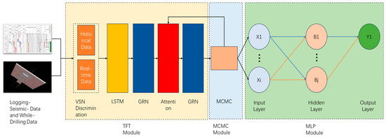
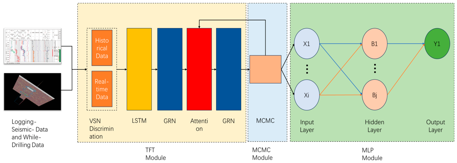
Finally, the single-value three formation pressures are calculated based on the well–seismic fused data generated by machine learning. The structure of the model is shown in Figure 5.

Figure 5. MLP-TFT-MCMC model structure.

In addition, the current mainstream vertical statistical calculation methods for formation tri-pressure that have credibility mostly adopt the normal distribution or uniform distribution as the core distribution model in the probability estimation stage. Combined with the actual geological conditions of deep formations in the southern margin block, such methods have obvious theoretical limitations. They cannot accurately characterize the true distribution of formation tri-pressure and exhibit poor adaptability. The specific deficiencies and improvement ideas are as follows.

The normal distribution is the most widely used probability estimation model. Its core principle is to assume that formation pressure samples follow a normal distribution. The mean and population variance are calculated based on samples, and the normal distribution probability density function is used to fit the sample distribution, thereby characterizing the distribution features of formation pressure. However, the application of this model relies on strict prerequisites: a large sample size and known population variance. This is significantly inconsistent with the actual working conditions of deep formations in the southern margin block, where measured pressure data are extremely scarce, representing a typical small-sample scenario. It not only fails to meet the large-sample requirement but also makes it difficult to obtain accurate population variance, resulting in considerable deviations between the probability fitting based on the normal distribution and the actual formation pressure distribution.

The uniform distribution serves as a supplementary probability estimation model. It assumes that formation pressure is uniformly distributed within the interval between the maximum and minimum measured values, independent of large samples and population variance. Nevertheless, this assumption contradicts the heterogeneity of deep formations in the southern margin block. The block features prominent lithological differences, large fluctuations in rock mechanical parameters and pressure distribution, and obvious concentration characteristics of pressure distribution. The equal-probability assumption of the uniform distribution cannot reflect such characteristics and thus also fails to accurately represent the true distribution law of formation tri-pressure.

To address the above theoretical deficiencies, this paper proposes introducing the t-distribution with adjustable degrees of freedom to improve the probability estimation module of the traditional vertical statistical method. The core improvement is to scientifically replace the normal distribution and uniform distribution based on the theoretical advantages of the t-distribution. The specific principle is as follows.

The probability density function of the original t-distribution is expressed as

$$f(x,n)={\displaystyle \frac{\Gamma \left(\frac{n+1}{2}\right)}{\sqrt{n\pi }\Gamma \left(\frac{n}{2}\right)}}{\left(1+{\displaystyle \frac{x^2}{n}}\right)}^{-{\displaystyle \frac{n+1}{2}}},\hspace{1em}-\infty <x<+\infty$$

where Γ(⋅) denotes the gamma function. For positive-integer arguments, Γ(k) = (k − 1)!, n is the sample size, and ν is the degree of freedom of the t-distribution. Its core adjustment rule is ν = n − 1, meaning that the degree of freedom adapts to the variation in formation pressure sample size. When the degree of freedom, ν, approaches infinity, the distribution approximates the normal distribution.

The improved expression is

$$f_T(x;\nu )={\displaystyle \frac{\Gamma \left(\frac{\nu +1}{2}\right)}{\sqrt{\nu \pi }\Gamma \left(\frac{\nu }{2}\right)}}{\left(1+{\displaystyle \frac{{(x-\overline{x})}^2}{\nu s^2}}\right)}^{-{\displaystyle \frac{\nu +1}{2}}}$$

where $\overline{x}$ is the mean of pressure samples within the sliding window, $\overline{x}={\displaystyle \frac{1}{n}}{\sum }_{i=1}^n{x}_i$, and s is the sample standard deviation within the sliding window, $s=\sqrt{{\displaystyle \frac{1}{n-1}}{\sum }_{i=1}^n{\left(x_i-\overline{x}\right)}^2}$.

Theoretically, the t-distribution can effectively compensate for the shortcomings of traditional distribution models. Its core advantages are reflected in three aspects: First, it does not require known population variance and can complete distribution fitting only using the sample mean and sample standard deviation within the sliding window, breaking through the strict prerequisites of large samples and known population variance for the normal distribution and perfectly matching the small-sample, scarce measured data conditions of deep formations in the southern margin block. Second, the degree of freedom can be adaptively adjusted. The smaller the sample size, the smaller the degree of freedom and the more significant the heavy-tailed characteristic of the t-distribution, which better fits the formation pressure distribution law in small-sample scenarios. Meanwhile, the degree of freedom can be further optimized by combining formation lithology, pressure-generating mechanisms and other features to adapt to pressure distribution fluctuations caused by formation heterogeneity. Third, it does not require a preset fixed distribution form and can autonomously fit the optimal probability distribution from measured samples. Compared with the prior assumptions of the normal and uniform distributions, it can more realistically reflect the randomness and uncertainty of deep formation pressure and accurately characterize the true distribution of formation tri-pressure.

2.3. Data Preprocessing

During drilling, logging and mud logging, data tend to contain considerable outliers and missing values, which can significantly affect model training results. Logging, mud logging, and logging-while-drilling (LWD) data have a high vertical resolution and can clearly reflect local microscopic characteristics, whereas seismic data have advantages in three-dimensional expansion and can effectively identify regional macroscopic characteristics. In this study, data from 8 drilled wells in the southern margin block are adopted, with a total of more than 100,000 data entries. Therefore, outlier removal and correlation analysis are performed on the raw data.

The main parameters are shown in Table 3 and Table 4.

Table 3. Extracted seismic attributes.

Serial Number	Seismic Attribute	Serial Number	Seismic Attribute	Serial Number	Seismic Attribute
1	3D curvature	15	Gradient magnitude	29	RMS amplitude
2	3D edge enhancement	16	Instantaneous bandwidth	30	Reflection intensity
3	Amplitude contrast	17	Interval velocity	31	Relative acoustic impedance
4	Apparent polarity	18	Instantaneous frequency	32	Remove bias
5	Average velocity	19	Instantaneous phase	33	Second derivative
6	Chaos	20	Instantaneous quality	34	Structural smoothing
7	Cosine of phase	21	Iso-frequency component	35	Sweetness
8	Dip deviation	22	Local flatness	36	Time gain
9	Dip illumination	23	Local structural azimuth	37	Trace AGC
10	Dominant frequency	24	Local structural dip	38	Trace AGC (iterative)
11	Edge evidence	25	Median filter	39	Trace gradient
12	Envelope	26	Original amplitude	40	t* attenuation
13	First derivative	27	Phase shift
14	Generalized spectral decomposition	28	Quadrature amplitude

Table 4. Logging, mud logging and logging-while-drilling data.

No.	Logging Data	No.	Mud Logging Data	No.	LWD Data
41	DEN	46	ROP	(LWD)
42	AC	47	WOB	56	LWD GR
43	GR	48	Rotary Speed	57	LWD AC
44	Resistivity	49	Torque	58	LWD DEN
45	Compensated Neutron	50	Outlet Temperature	Other LWD Data
		51	Inlet Temperature	59	PWD
		52	Hook Load	60	Near-Bit Rotary Speed
		53	Weight Indicator
		54	Outlet Density
		55	Inlet Density

These data are affected by many factors during acquisition, resulting in missing values and outliers, as well as serious noise spikes in the data curves. To eliminate such interference and retain data that can correctly represent formation properties, the unascertained filtering method and the five-point function smoothing method are adopted for data processing.

The unascertained filtering method calculates the unascertained degree of each data point, performs trend fitting using parameters within the neighborhood, and replaces outliers with the mathematical expectation [16,17]. Its formula is as follows:

$$\mathrm{A}=\left[\left[\underset{1⩽\mathrm{i}⩽\mathrm{n}}{\mathrm{m}\mathrm{i}\mathrm{n}}{\mathrm{X}}_{\mathrm{i}},\underset{1⩽\mathrm{i}⩽\mathrm{n}}{\mathrm{m}\mathrm{a}\mathrm{x}}{\mathrm{X}}_{\mathrm{i}}\right],\mathrm{\phi }\left(\mathrm{t}\right)\right]$$

$$\phi \left(t\right)=\left\{\begin{array}{l}{\displaystyle \frac{{\xi }_i}{{{\displaystyle \sum }}_{i=1}^n{\xi }_i}},t=X_i\left(i=1,2,\cdots n\right)\hfill \\ 0\hfill \end{array}\right.$$

where ${\xi }_i$ is the weight at each depth $X_i$.

Given the complex nonlinear relationships among drilling, logging, mud logging, and seismic data, it is necessary to consider actual formation lithology, abnormal high pressure, and other conditions. After comprehensive consideration, this paper adopts the Maximal Information Coefficient (MIC) method to analyze the correlation between data. The calculation formula is as follows:

$$\mathrm{MIC}\left[x,y\right]=\underset{\left|X\right|\left|Y\right|<\mathrm{B}}{\max }{\displaystyle \frac{I\left[X,Y\right]}{{\log }_2\left(\min \left(\left|X\right|,\left|Y\right|\right)\right)}}$$

$$I\left[X,Y\right]={\displaystyle \sum }_{X,Y}p\left(X,Y\right){\log }_2{\displaystyle \frac{p\left(X,Y\right)}{p\left(X\right)p\left(Y\right)\prime }}$$

where $\mathrm{MIC}\left[x,y\right]$ is the correlation coefficient between variables x and y; X and Y are the discrete vectors of variables x and y, respectively; B is the division threshold of discrete grids in two-dimensional space, which is generally the 0.6th power of the sample data size; and $p\left(X\right)$, $p\left(Y\right)$, and $p\left(X,Y\right)$ represent the probabilities that a data point is in the X-th column, Y-th row, and X-th column and Y-th row of the divided two-dimensional discrete grids, respectively.

3. Results

Rock mechanical parameters and in situ stress calculation models are used to calculate and statistically analyze the distribution of each formation group in the southern margin area, as shown in Table 5 and Table 6. It can be seen that the stress in the K2d is relatively concentrated and shows a downward trend, and all parameters of the J3q show a downward trend. This indicates that these two formations have significant uncertainty and are prone to drilling risks.

Table 5. Calculation results for Poisson’s ratio and Young’s modulus.

Formation	Poisson’s Ratio Range	Poisson’s Ratio Probability Maximum Value	Young’s Modulus Range (GPa)	Young’s Modulus Probability Maximum (GPa)
Q	0.26~0.33	0.305	11~35	11.4
N2d	0.20~0.35	0.290	7~50	13.5
N1t	0.24~0.32	0.260	12~47	18.3
N1j	0.24~0.31	0.270	13~45	26.5
E2-3a	0.24~0.34	0.316	15~45	17.3
E1-2z	0.25~0.31	0.265	17~34	31.2
K2d	0.23~0.28	0.252	25~48	35.7
Lmq + sjk	0.24~0.28	0.243	26~48	36.8
K1h	0.26~0.27	0.243	26~45	34.5
K1q	0.23~0.26	0.252	30~57	32.2

Table 6. Calculation results for in situ stress.

Formation	Maximum In Situ Stress (g/cm3)	Maximum Probability (g/cm3)	Minimum In Situ Stress (g/cm3)	Maximum Probability (g/cm3)
Q	1.75~2.26	2.11	1.49~2.03	1.79
N2d	1.69~2.20	2.01	1.21~2.02	1.46
N1t	1.69~2.05	1.86	1.21~1.78	1.45
N1j	1.74~2.05	1.86	1.25~1.80	1.53
E2-3a	1.74~2.27	2.09	1.12~2.01	1.80
E1-2z	1.75~2.20	1.88	1.21~1.97	1.39
K2d	1.56~1.91	1.78	1.09~1.75	1.35
Lmq + sjk	1.56~1.96	1.65	1.09~1.64	1.54
K1h	1.64~1.96	1.92	1.18~1.64	1.56
K1q	1.44~1.94	1.83	0.91~1.76	1.61

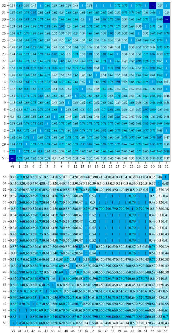
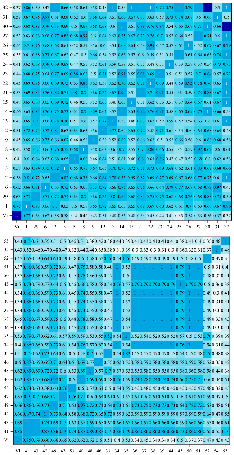
During the correlation analysis, complex seismic attributes used for fracture identification (Nos. 4, 7, 10, 11, 16, 18, 19, 20, and 28) were removed, and the remaining 46 logging, mud logging and seismic attributes were analyzed. Considering that the 46 × 46 matrix is excessively large, the correlation analysis with interval velocity was carried out in two separate steps.

Selecting an appropriate MIC threshold is critical for model prediction. An MIC threshold that is too low will result in excessive low-correlation features being included in model training and prediction, while an excessively high MIC threshold will leave too few available features. Generally, two features are considered to be highly correlated if the MIC value is greater than 0.5. In this study, parameters with an MIC value greater than 0.6 are selected. As shown in Figure 6, the final dataset consists of 10 optimized parameters, including interval transit time, gamma ray, formation density, rate of penetration (ROP), weight on bit (WOB), hook load, rotary speed, chaos, RMS amplitude, and 3D curvature. Each parameter corresponds to depth one-to-one, and the output is interval velocity. The logging-while-drilling (LWD) data mainly include LWD interval transit time and LWD gamma ray, which are updated in a constrained manner. A total of 334,543 data points from eight drilled wells in the southern margin block are used to construct the dataset, covering all depth points of these wells. Furthermore, the adoption of the MIC threshold of 0.6 effectively balances feature retention and redundant information elimination. It avoids introducing a large number of weakly correlated interfering features that may cause model overfitting under a lower threshold and also prevents the loss of valuable logging and geological characteristic information caused by an overly strict threshold. The 10 screened optimized parameters maintain good physical interpretability and nonlinear correlation with the target formation parameters, which can significantly improve the training efficiency, prediction accuracy and generalization stability of the subsequent MLP–TFT–MCMC prediction model.

Figure 6. Correlation analysis results.

To evaluate the prediction accuracy and temporal updating performance of the model, commonly used evaluation metrics include the Mean Absolute Error (MAE) and the Root Mean Squared Error (RMSE).

The Mean Absolute Error adopts the form of absolute error, which is more robust to outliers and can directly reflect the average prediction deviation of the model with clear physical significance:

$$\mathrm{MAE}={\displaystyle \frac{1}{N}}{\displaystyle \sum _{i=1}^N|}{y}_i-{\widehat{y}}_i|$$

The Root Mean Squared Error is the arithmetic square root of the Mean Squared Error, which has the same dimension as the original data and facilitates intuitive interpretation of the actual magnitude of the prediction error:

$$\mathrm{RMSE}=\sqrt{{\displaystyle \frac{1}{N}}{\displaystyle \sum _{i=1}^N{(y_i-{\widehat{y}}_i)}^2}}$$

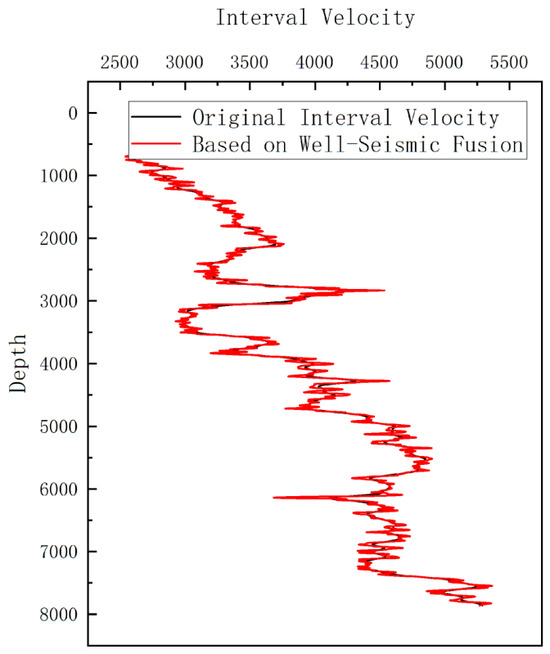
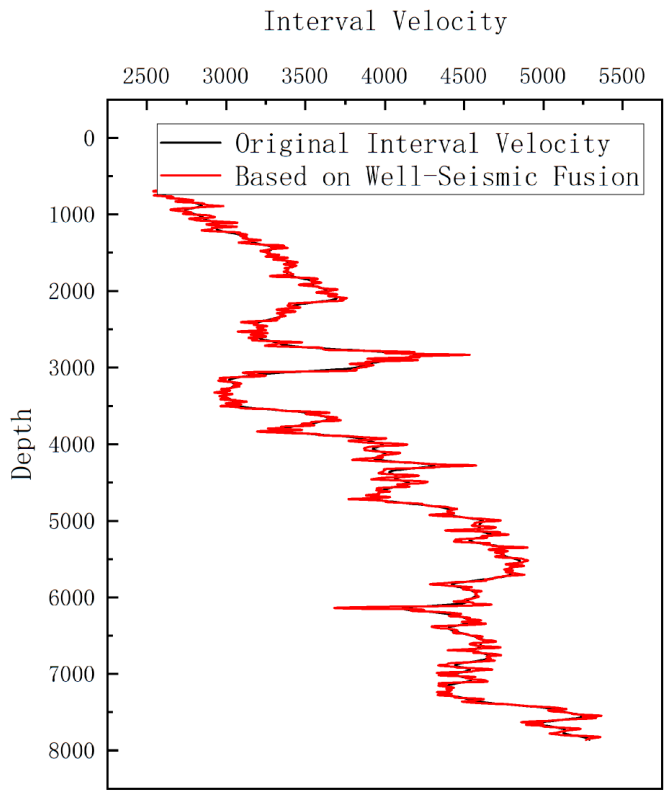
A comparison chart of the well–seismic fusion data and the data obtained via the traditional method described in the previous section is presented in Figure 7. It can be seen that the formation interval velocity constructed based on well–seismic fusion not only inherits the macroscopic continuity of seismic data in the vertical direction but also retains the high precision of logging and mud logging data. Quantitative error analysis shows that the well–seismic fusion method achieves a Mean Absolute Error (MAE) of 0.08 and a Root Mean Squared Error (RMSE) of 0.11, which are significantly lower than those of the conventional single-data approach. It can better reflect formation characteristics and lays a foundation for the subsequent uncertainty analysis of formation information.

Figure 7. Comparison chart of interval velocity constructed based on well–seismic fusion for well X.

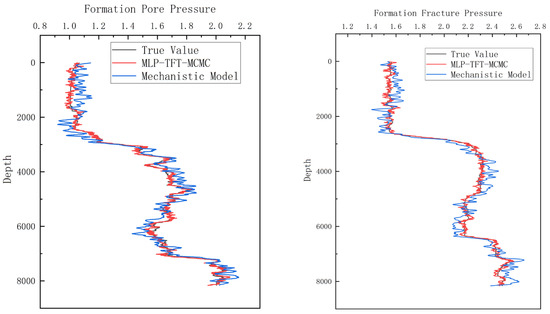
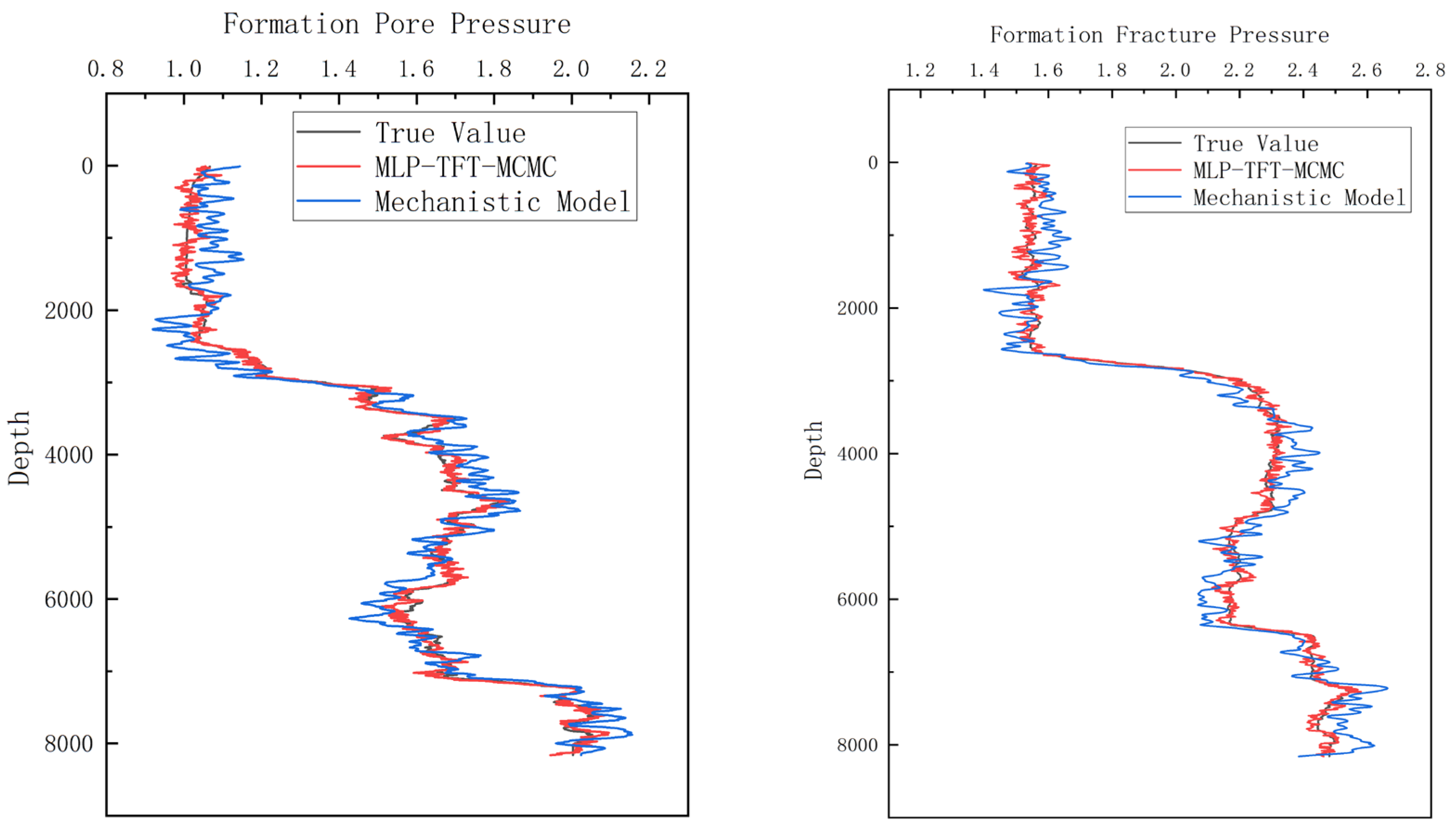
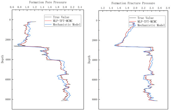
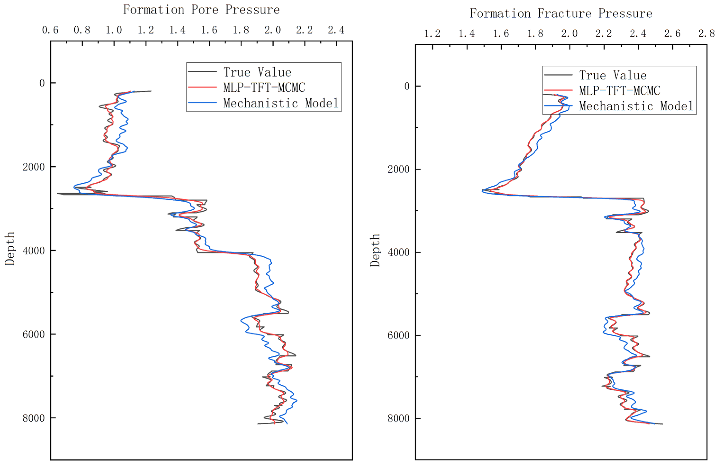
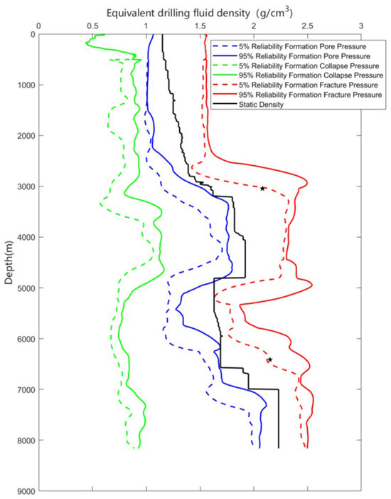
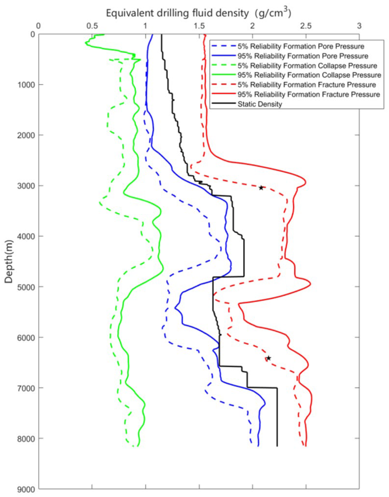
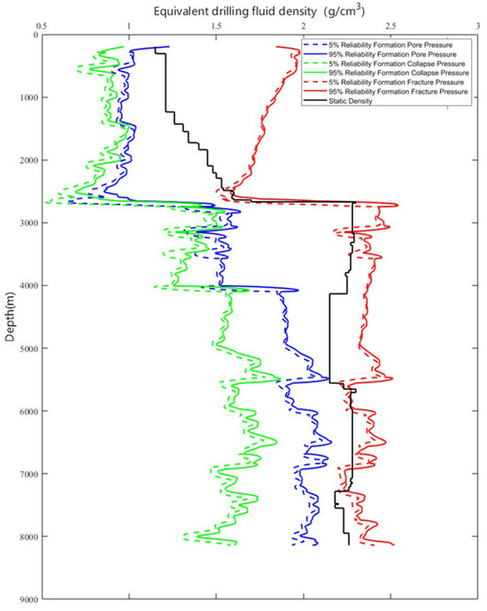
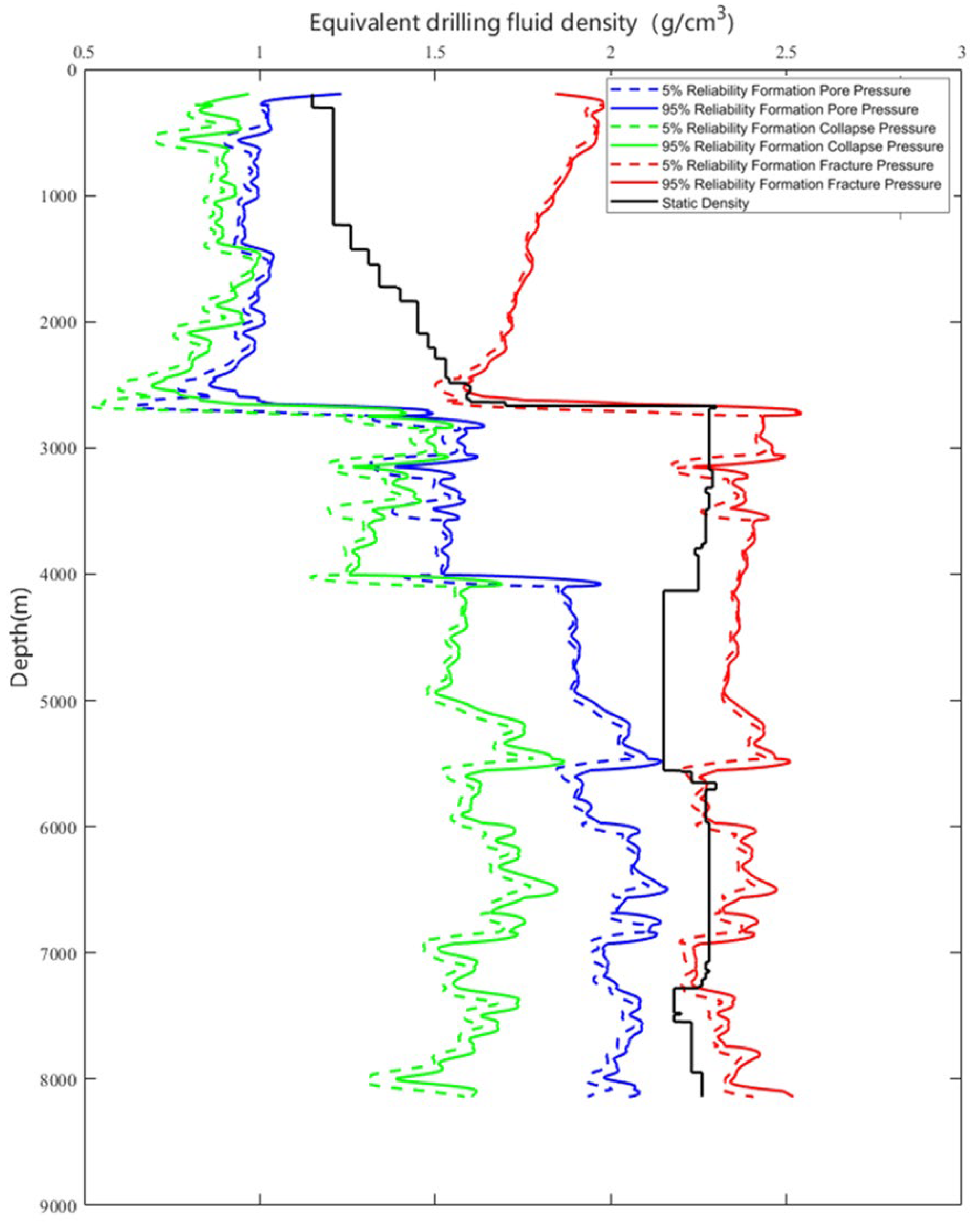
Here, the single-value formation pore pressure is taken as an example for verification. As shown in Figure 8 and Figure 9, the prediction based on the MLP-TFT-MCMC machine learning model and well–seismic fusion method is more accurate than that of the traditional mechanism model. Quantitative error evaluation indicates that the traditional mechanism model yields an MAE of 0.16 and an RMSE of 0.21, while the proposed hybrid model reduces the MAE to 0.05 and the RMSE to 0.07. Compared with the traditional mechanism model, the MAE is reduced by approximately 68.75% and the RMSE is reduced by approximately 66.67%, demonstrating a remarkable improvement in prediction accuracy. The improved method for predicting three formation pressures with confidence levels was applied to Well X in the southern margin area, and the results were verified against actual formation breakdown tests. The casing program of Well X is listed in Table 7. It was found that this method can accurately predict the three formation pressures, and the results are shown in Figure 10 and Figure 11.

Figure 8. Comparison of formation pore pressure and fracture pressure calculated by different methods in Well X.

Figure 9. Comparison of formation pore pressure and fracture pressure calculated by different methods in Well Y.

Table 7. X wellbore structure and drilling fluid density.

Schedule an Appointment	Depth/m	Drilling Fluid Density/(g/cm3)	Ground-Breaking Test
First spud	200	1.15
Second spud	2800	1.15–1.45
Third spud	5000	1.45–2	3175/2.25 (unfractured)
Fourth spud	6500	1.74–1.69
Fifth spud	7950	1.69–2.23	6604/2.4 (unfractured)

Figure 10. Formation tri-pressure with confidence level of Well X. Asterisk denotes measured pressure data points.

Figure 11. Formation tri-pressure with confidence level of Well Y.

4. Conclusions

Aiming at the prominent problems of high uncertainty in formation information and severe potential risks faced in ultra-deep well drilling in the southern margin of the Junggar Basin, the Fan Honghai and Huang Rongzun models were selected to calculate and analyze the rock mechanical parameters and in situ stress distributions of different formations in this area. It was found that formation information exhibits considerable uncertainty in the Donggou Formation and the lower part of the Qingshuihe Formation. Therefore, a formation pressure prediction method with confidence levels is introduced to quantitatively characterize the uncertainty of formation information. Furthermore, the confidence-based calculation method is improved by means of well–seismic fusion and the constructed MLP-TFT-MCMC hybrid model. Quantitative verification shows that the well seismic fused interval velocity achieves an MAE of 0.08 and an RMSE of 0.11. For formation pore pressure prediction, the traditional mechanism model delivers an MAE of 0.16 and an RMSE of 0.21, while the proposed hybrid model reduces the MAE to 0.05 and the RMSE to 0.07, representing a reduction of approximately 68.75% in MAE and 66.67% in RMSE. The applicability of the proposed method in this area is verified using formation breakdown test data and actual drilling fluid density from well history records.

In summary, the confidence-based prediction method for three formation pressures proposed in this paper provides an effective technical approach to alleviate the challenges of high formation information uncertainty and difficulty in precise risk prevention and control for ultra-deep wells in the southern margin of the Junggar Basin. With significantly reduced prediction errors and remarkably improved accuracy, this method offers a valuable theoretical reference and engineering support for the safe and efficient exploration and development of oil and gas resources in this region. It should be emphasized that this method is applicable to the southern margin ultra-deep wells with similar geological characteristics, and the prediction accuracy is supported by multi-well verification and statistical tests. Due to the constraints of assumptions and data conditions, the model still has certain limitations, and the conclusions are not universally extended to all geological scenarios. Further, this study has obvious limitations that need to be addressed. Firstly, the current model does not consider the influence of natural fractures, fault zones and related structural factors, which may affect the prediction accuracy in areas with complex structural conditions. Secondly, the applicability of the proposed method in scenarios with insufficient high-quality seismic data and ultra-deep formations has not been fully verified, and its adaptability in such complex environments remains to be further explored; these unresolved issues may lead to partial deviations in the conclusions under specific conditions. Future work should incorporate fault-controlled stress heterogeneity and frictional slip behavior into the modeling framework to better capture the coupled mechanical–hydraulic response near fault zones. Meanwhile, follow-up studies will collect more comprehensive data, expand the verification scope, and further test and improve the applicability of the method in scenarios with insufficient seismic data and ultra-deep complex formations so as to enhance the rigor and universality of the research results.

References

- He, L.C.; Tang, B. The Up-to-Date Technologies of Ultra-Deep Well Drilling in Junggar Basin and Suggestions for Further Improvements. Pet. Drill. Tech. 2022, 50, 1–8. [Google Scholar]
- Hottman, G.E.; Johnson, R.K. Estimation of Formation Pressures from Log-Derived Shale Properties. J. Pet. Technol. 1965, 17, 717–722. [Google Scholar] [CrossRef] [Scilit]
- Yu, J.Q.; Sun, X.P.; Yu, Y.C.; Li, X.; Li, X.M.; Xu, G.C. Research Progress on Deep Formation Pressure Prediction Technology. Mar. Orig. Pet. Geol. 2024, 29, 337–347. [Google Scholar]
- Liu, J.N. Discussion on Early Warning Technology for Oil Drilling Engineering Accidents. China Pet. Chem. Stand. Qual. 2020, 40, 159–162+165. [Google Scholar]
- Zhang, J.C. Research on Formation Pressure Prediction Based on Physics-Data Dual-Driven. Master’s Thesis, China University of Petroleum, Beijing, China, 2022. [Google Scholar]
- Shi, X.; Cai, J.; Cheng, Y.; Li, L. Estimating Pore Pressure in HPHT Wells in Yinggehai Basin, China Based on Hierarchical Eaton’s Method. Adv. Mater. Res. 2012, 347, 3–9. [Google Scholar] [CrossRef] [Scilit]
- Hutomo, P.S.; Rosid, M.S.; Haidar, M.W. Pore Pressure Prediction Using Eaton and Neural Network Method in Carbonate Field “X” Based on Seismic Data. IOP Conf. Ser. Mater. Sci. Eng. 2019, 546, 032017. [Google Scholar] [CrossRef] [Scilit]
- Oloruntobi, O.; Adedigba, S.; Khan, F.; Chunduru, R.; Butt, S. Overpressure Prediction Using the Hydro-Rotary Specific Energy Concept. J. Nat. Gas. Sci. Eng. 2018, 55, 243–253. [Google Scholar] [CrossRef] [Scilit]
- Fan, H.H. Discussion on Traditional Methods for Detecting Formation Pore Pressure from Log Data. Pet. Explor. Dev. 2003, 30, 72–74. [Google Scholar]
- Fan, H.H.; Zhang, C.J. Reasonable Calculation and Fitting Method of Overburden Pressure Gradient. Pet. Drill. Tech. 2002, 30, 6–8. [Google Scholar]
- Yang, J. Study on BP Network Prediction Method of Formation Pressure and Its Application. Oil Drill. Prod. Technol. 2003, 25, 13–15. [Google Scholar]
- Keshavarzi, R.; Jahanbakhshi, R. Real-Time Prediction of Pore Pressure Gradient Through an Artificial Intelligence Approach: A Case Study from One of Middle East Oil Fields. Eur. J. Environ. Civ. Eng. 2013, 17, 675–686. [Google Scholar] [CrossRef] [Scilit]
- Ahmed, A.; Elkatatny, S.; Ali, A.; Mahmoud, M.; Abdulraheem, A. New Model for Pore Pressure Prediction While Drilling Using Artificial Neural Networks. Arab. J. Sci. Eng. 2019, 44, 6079–6088. [Google Scholar] [CrossRef] [Scilit]
- Song, X.Z.; Yao, X.Z.; Li, G.S.; Xiao, L.; Zhu, Z. Calculation Method of Formation Pore Pressure Based on LSTM-BP Neural Network. Pet. Sci. Bull. 2022, 7, 12–23. [Google Scholar]
- Yu, W.W.; Wang, X.Y.; Done, J.X.; Lv, L.; Liu, Y.C. Well-Seismic Integration Technology Based on MLP Deep Learning Curve Reconstruction; Petroleum Geophysical Exploration Committee of China Petroleum Society. In Proceedings of the 2nd China Petroleum Geophysical Exploration Annual Conference; Overseas Business Department of Research Institute, BGP Inc.: Zhuozhou, China, 2024; Volume 2, pp. 124–127. [Google Scholar]
- Guan, Z.C.; Sheng, Y.N.; Xu, Y.Q.; Wang, Q.; Zhang, B. Dynamic Drilling Risk Assessment Method Based on PSO-Optimized BP Neural Network. J. Saf. Sci. Technol. 2017, 13, 5–11. [Google Scholar]
- Guan, Z.C.; Ke, K.; Lu, B.P. Method for Determining Casing Stages and Setting Depth under Pressure Uncertainty. J. China Univ. Pet. (Nat. Sci. Ed.) 2009, 33, 71–75. [Google Scholar]
- Sheng, Y.N.; Guan, Z.C.; Wei, K.; Zhao, T. Casing Program Optimization Method Based on Pre-Drilling Risk Prediction. Oil Drill. Prod. Technol. 2016, 38, 415–421. [Google Scholar]
- Lu, T.M.; Ye, C.; Lu, X.M.; Rong, K.S.; Liu, K.C.; Yao, X.Y.; Zhou, Z.N. Mechanism and Countermeasures of Borehole Instability in High-Temperature Organic Matter Reservoirs in Southern Margin of Junggar Basin. Xinjiang Oil Gas. 2022, 18, 26–31. [Google Scholar]
- Yang, H.; Chen, H.; Li, Y.L.; Sun, W.G.; Zhou, P.G. Optimization and Application of Strength Criteria for Mechanical Instability Evaluation of Drilling Borehole. Xinjiang Oil Gas. 2022, 18, 1–5. [Google Scholar]
- Shen, X.P.; Xiang, D.M.; Wu, X.Y. Integrated 3D In-Situ Stress and Single-Well Geomechanics Calculation and Application. Xinjiang Oil Gas. 2023, 19, 40–48. [Google Scholar]
- Li, Y.; Yang, J.; Yu, Q.; Liu, X.; Guo, W.; Miao, S. 3D coupled dynamic modeling of deep shaft excavation near a fault: Coseismic slip and seismic hazards. J. Rock. Mech. Geotech. Eng. 2025; in press.
- Li, Y. Spatial distribution of strain energy changes due to mining-induced fault coseismic slip: Insights from a rockburst at the Yuejin coal mine, China. Rock. Mech. Rock. Eng. 2025, 58, 1693–1706. [Google Scholar] [CrossRef] [Scilit]
- Li, Y.; Yang, J.; Gao, X. Fault slip amplification mechanisms in deep mining due to heterogeneous geological layers. Eng. Fail. Anal. 2025, 169, 109155. [Google Scholar] [CrossRef] [Scilit]
- Li, Y.; Fukuyama, E.; Yoshimitsu, N. Comprehensive 3-D modeling of mining-induced fault slip: Impact of panel length, panel orientation, and far-field stress orientation. Rock. Mech. Rock. Eng. 2025, 58, 5961–5979. [Google Scholar] [CrossRef] [Scilit]
- Li, Y.; Gao, X. Assessment of variations in shear strain energy induced by fault coseismic slip in deep longwall mining. Int. J. Coal Sci. Technol. 2025, 12, 3–16. [Google Scholar] [CrossRef] [Scilit]
- Lu, R. Study on Rock Mechanical Parameters and In-Situ Stress Characterization Methods of Shale Reservoirs. Master’s Thesis, China University of Geosciences, Beijing, China, 2021. [Google Scholar]
- Chen, M.; Jin, Y.; Zhang, G.Q. Rock Mechanics in Petroleum Engineering; Science Press: Beijing, China, 2008; pp. 21–27+303–305. [Google Scholar]
- Jing, Y.; Wang, T.; Zhang, B.; Zheng, Y.; Li, X.; Lu, N. Safety Risk Analysis of Well Control for wellbore with sustained annular pressure and Prospects for Technological Development. Chem. Technol. Fuels Oils 2025, 61, 110–119. [Google Scholar] [CrossRef] [Scilit]
- Zhang, B.; Zhao, J.; Sun, J.; Lu, N.; Liao, H.; Zhang, Q.; Sun, T. Explanation of Tie-Back Cement Sheath Leakage Caused by Microannulus in Ultra-Deep Gas Wells and Control Strategy. Energy Technol. 2026, 14, e202502342. [Google Scholar] [CrossRef] [Scilit]
- Xu, Y.Q.; He, B.L.; Wang, S.; Han, C.; Xiao, F.; Guan, Z.C.; Liu, K. Formation Pore Pressure Prediction Method Driven by Deep Learning and Eaton’s Method. J. China Univ. Pet. (Nat. Sci. Ed.) 2023, 47, 50–59. [Google Scholar]
- Xu, Y.Q.; Guan, Z.C.; Zhang, H.N.; Zhang, H.Z. Fine Casing Program Design Method Based on Formation Pressure Profile with Confidence Level. J. China Univ. Pet. (Nat. Sci. Ed.) 2014, 38, 72–77. [Google Scholar]
- Sheng, Y.N.; Guan, Z.C.; Zhao, T.F.; Ye, L. Study on Formation Pressure Calculation Method with Confidence Level. Sci. Technol. Eng. 2016, 16, 37–42. (In Chinese) [Google Scholar]
Disclaimer/Publisher’s Note: The statements, opinions and data contained in all publications are solely those of the individual author(s) and contributor(s) and not of MDPI and/or the editor(s). MDPI and/or the editor(s) disclaim responsibility for any injury to people or property resulting from any ideas, methods, instructions or products referred to in the content. |
© 2026 by the authors. Licensee MDPI, Basel, Switzerland. This article is an open access article distributed under the terms and conditions of the Creative Commons Attribution (CC BY) license.