Article

Data-Driven Analysis of the Effectiveness of Water Control Measures in Offshore Horizontal Wells

1
Caofeidian Operation Company, CNOOC (China) Co., Ltd., Tianjin 300000, China
2
Key Laboratory for Enhanced Oil Recovery, CNOOC Energy Technology & Services Limited, Tianjin 300452, China
3
CNOOC EnerTech-Drilling & Production Co., Tianjin 300452, China
4
State Key Laboratory of Offshore Oil and Gas Exploitation, Tianjin 300452, China
5
School of Petroleum and Natural Gas Engineering, Changzhou University, Changzhou 213164, China
*
Author to whom correspondence should be addressed.
Processes 2026, 14(1), 88; https://doi.org/10.3390/pr14010088
Submission received: 31 October 2025 / Revised: 8 December 2025 / Accepted: 16 December 2025 / Published: 26 December 2025

Abstract

Implementing effective water control measures in horizontal wells is essential for sustaining stable production in offshore oilfields. However, due to complex reservoir geological characteristics and diverse water control technologies, significant variability exists in the effectiveness of such measures, posing challenges for strategy selection. To address this gap, this study establishes a comprehensive and standardized multi-dimensional indicator system for describing treated wells, integrating geological, operational, and production parameters—an aspect seldom systematized in previous research. A major innovation of this work lies in developing a hybrid correlation evaluation framework that combines Pearson, Spearman, and canonical correlation analyses, enabling a more robust quantification of the relationships between influencing factors and water control effectiveness. This framework not only identifies the dominant indicators but also mitigates the limitations of single-method correlation analysis. Building upon these insights, the study proposes a machine learning-driven prediction system using Random Forest and Gradient Boosting algorithms, achieving classification accuracy exceeding 80% and effective regression prediction of measure duration. This represents a practical advancement over traditional empirical or single-feature decision approaches. The results reveal that overall field water cut percentage, 30-day pre-treatment water cut percentage, and daily liquid production are the key indicators governing treatment performance. Furthermore, water control measures in edge water reservoirs show significantly better performance than those in bottom water reservoirs. The developed prediction model provides a generalizable, data-driven decision-support tool, offering significant value for optimizing water control technologies in offshore horizontal wells.

1. Introduction

Offshore oilfield production faces a series of challenges, including premature water breakthrough in horizontal wells, severe water encroachment, and high water cut percentage. These issues severely impact the production efficiency and economic benefits of oilfields, urgently requiring effective water control measures for their resolution [1,2,3]. Due to their unique advantages in design and operation, horizontal wells have been widely applied in offshore oilfields. However, the problem of premature water breakthrough in horizontal wells continues to severely restrict oilfield production stability and economic benefits [4]. Therefore, adopting effective water control measures in horizontal wells to ensure long-term stable oilfield production has become a critical issue that urgently needs to be addressed.
In recent years, significant research advancements have been made both domestically and internationally regarding horizontal well water control technologies. Various technical means have been proposed to address water encroachment, such as water shutoff techniques, polymer gel plugging and mechanical water shutoff [5]. While these technologies have achieved some progress, their effectiveness is often influenced by multiple factors, including reservoir characteristics, wellbore structure, and production operations [6]. The actual conditions of different horizontal wells vary significantly, leading to considerable uncertainty in the effectiveness of water control and measures [7,8,9,10]. Therefore, conducting sensitivity analysis of key factors influencing the effectiveness of water control and measures is crucial for formulating more scientific and effective water control strategies.
Investigating the sensitivity of factors affecting the effectiveness of water control measures can not only provide an important basis for optimizing production schemes but also improve the application efficiency of water shutoff technologies and extend the production life of horizontal wells. By thoroughly analyzing these key factors, more precise and economical water control solutions can be tailored for different oilfields, thereby enhancing oilfield production performance and resource management levels.
The main innovations of this study are as follows:
(1)
A multi-dimensional data-driven evaluation framework is established for the first time to quantitatively assess the effectiveness of water control measures in offshore horizontal wells. By integrating geological, operational, and production parameters, the proposed method captures both static and dynamic influencing factors.
(2)
The study introduces a comprehensive correlation and sensitivity analysis approach combining Pearson, Spearman, and canonical correlation analyses, revealing the dominant variables that govern the effectiveness of different water control strategies.
(3)
A hybrid prediction model based on multiple machine learning algorithms (Logistic Regression, Random Forest, Gradient Boosting) is constructed to achieve high-accuracy effectiveness classification and duration regression prediction, offering data-driven decision support for offshore field management.
The overall structure of this paper is organized as follows: Section 3 describes the dataset construction and indicator system. Section 4 presents methods for analyzing sensitive factors and establishing machine learning models. Section 5 presents the sensitivity analysis of influencing factors and their correlation characteristics. Section 6 establishes the prediction models and analyzes their performance. Finally, Section 7 summarizes the main conclusions and provides suggestions for the optimization of water control measures.

2. Related Work

The challenge of water control in horizontal wells has been widely studied, with research evolving from engineering techniques and mechanistic modeling to more advanced data-driven approaches.
From a technological perspective, a variety of chemical and mechanical water shutoff methods have been developed. Randy [1] provided a comprehensive review of water shutoff and conformance improvement, summarizing key developments in wellbore isolation and reservoir conformance techniques. Sun [2] systematically discussed the mechanisms and field performance of horizontal well water shutoff methods, including polymer gels and chemical plugging agents. Abdullah [5] compared chemical and mechanical treatments in offshore applications, highlighting their advantages and limitations under different geological conditions. For specific challenges such as water coning in heavy oil reservoirs, Qu [6] investigated the use of soft polymer gels, demonstrating improved plugging performance and enhanced oil recovery in offshore cold production environments.
Mechanistic modeling and numerical simulation have been essential for understanding water invasion and relative permeability modification. Fatemeh [7] applied numerical models to analyze influencing factors and treatment efficiency, while Tileuberdi [8] summarized the technical difficulties of gel treatments in field implementation. In addition, Liu [11] examined segmented production and compound water control technologies in bottom-water reservoirs at ultra-high water cut percentage stages.
Despite these advances, the effectiveness of water control operations remains highly variable and dependent on complex, interrelated parameters. Few studies have systematically integrated multi-dimensional statistical sensitivity analysis with machine learning prediction for evaluating the effectiveness of water control measures in offshore horizontal wells. To address this gap, the present study develops a comprehensive indicator system and a closed-loop data-driven framework that connects factor sensitivity evaluation with predictive modeling, providing quantitative and interpretable decision support for water control measure optimization. Beyond the oil and gas domain, similar multi-indicator evaluation and optimization frameworks have been successfully applied in other resource-exploitation fields. For example, Zou [12] developed a Bayesian-network-based evaluation model combined with Cuckoo Search optimization to assess coordinated exploitation of coal and coalbed methane, demonstrating the broader applicability of data-driven intelligent evaluation approaches.

3. Sample Set Preparation

3.1. Data Sources

This study’s dataset was collected from 31 high water-cut old wells in off-shore oilfields where water control measures were implemented between 2007 and 2024. These oil wells are from an offshore oil field in northern China, with a well spacing of about 300 m, a horizontal section length of about 400 m, a permeability ranging from 2000 mD to 4500 mD, a viscosity ranging from 50 mPa · s to 350 mPa · s, and a bottom depth ranging from 2000 m to 3000 m. Relevant data were obtained from diverse sources, including daily well development data and reservoir geological parameters for each treated well. Specifically, the daily well development data include daily pre- and post-measure production figures for each well, encompassing daily oil output, daily water output, and water percentage. Reservoir geological parameters include information such as the sand body (sandstone), reservoir type, formation oil viscosity, and information on the positioning of the treated wells within the reservoir block. Following the collection of data, cleaning was performed to ensure precision. Through verification in consultation with the oilfield, missing values were filled, and outliers were rectified, ensuring data accuracy. Missing values were corrected using domain knowledge and temporal interpolation. Outliers were detected using the 1.5 × IQR rule and validated through field engineer consultation before being replaced or removed.

3.2. Establishment of Indicator System

Each treated well involves a large number of data indicators that need to be considered. When exploring the influencing factors of measure effectiveness and conducting sensitivity analysis, it is crucial to focus on those data indicators that significantly impact the performance of high water-cut wells. The accuracy of data mining is closely related to the quality of sample data. If too many irrelevant factors are analyzed simultaneously, it will not only increase workload and computational burden but also potentially lead to dimensionality overload [13]. Furthermore, incorporating irrelevant numerical indicators may introduce substantial interference and noise, thus affecting the accuracy of data mining results. Therefore, constructing a scientific and reasonable indicator system is particularly important. This not only ensures that crucial feature indicators are not overlooked but also reduces computational complexity while excluding irrelevant features [14,15].
Based on the actual collected data from treated wells in the oilfield, combined with expert practical experience and reservoir engineering theoretical knowledge, an indicator system for analyzing measure effectiveness was established. This system includes reservoir geological parameters, water control measures, 30-day production data before and after the measures, and a comparative analysis of production metrics pre- and post-intervention. Table 1 presents the definitions and ranges of these indicators. As shown in Table 1, reservoir geological parameters include reservoir type (edge water reservoir or bottom water reservoir) [16], sand body, and formation crude oil viscosity. There are nine categories of water control techniques: AICD, ICD + Particle Packing [17], Water Shutoff—ACP, Water Shutoff—Cement, Well Shut-in for Pressure Cone Management, Chemical Water Shutoff [18], Downhole Oil–water Separation, Open-Hole Compartmentalized Water Control, and Central Tubing Completion. The 30-day production data before and after the measures include daily liquid production, daily oil production, and water cut percentage. Comparisons of production data before and after the measures include daily liquid production reduction, daily water production reduction, water cut percentage comparison, daily oil increment (industry standard method) daily oil increment (net water cut percentage reduction method), and daily oil increment (constant liquid production method). In addition to the names of the indicators, Table 1 also provides their definitions and units. It is worth noting that taking into account the dynamic trends of the production curve before measures and the time-series patterns containing key predictive information may have a significant impact on the selection of water control measures and the evaluation of their effectiveness. However, due to the limitations of oilfield data collection, these considerations have not been included in the scope of this study. It is expected that more representative research results will be obtained in the future.

3.3. Construction of Indicator System

In response to the research needs, the collected 31 historical water control data were further processed and divided into three categories of information: geological development characteristics, water control measures characteristics, and measure effectiveness characteristics [19]. Specifically, the geological development characteristics include geological information related to reservoirs, sand bodies, and other factors; the water control measures characteristics involve the types of different processes used; and the measure effectiveness characteristics reflect the actual performance of various water control measures in practice. The relevant sample parameters are shown in Table 2.
To ensure objective and reproducible sample labeling, this study quantitatively defines the “effectiveness” and “validity” of water control measures. Effectiveness refers to the improvement observed within 30 days after the treatment and is classified as effective when both the water cut percentage decreases by at least 5 percentage points and the daily oil production increases by no less than 2 m3/d; otherwise, the measure is considered ineffective. Validity is defined as the continuous duration during which the treatment maintains its effect, measured by the number of days that the water cut percentage remains at least 3 percentage points lower than the pre-treatment level or the daily oil production remains at least 1 m3/d higher than before the treatment. These quantitative criteria minimize subjective judgment and ensure consistency in the evaluation of water control performance [20,21,22].

4. Methodology

4.1. Correlation and Sensitivity Analysis Methods

This section aims to identify and quantify the key factors that influence the effectiveness of water control measures. By employing correlation and sensitivity analysis methods, including Pearson, Spearman, and canonical correlation analyses, the interrelationships between geological, operational, and production parameters are systematically evaluated.
Pearson correlation coefficients (PCC) are suitable for normally distributed data exhibiting normal distribution. Spearman analysis is primarily used for variables failing to satisfy normality or for variables with an unknown distribution type. PCC are predominantly employed to assess linear relationships, whereas Spearman coefficients are chiefly applied to evaluate monotonic relationships [23,24].
Pearson correlation coefficients (PCC) indicate the intensity of linear associations between two variables. Higher absolute values denote stronger correlations, and the direction indicates the nature of the relationship. As summarized in Table 3, the magnitude of the coefficient is categorized to quantify the strength of the linear relationship, adapted from established statistical standards. Crucially, a coefficient ρX, Y = 0 signifies the absence of a linear relationship but does not imply independence, as the variables may still exhibit a strong non-linear or curvilinear association.
While Pearson correlation analysis is designed to measure the linear relationship between two variables, the Spearman method assesses their monotonic relationship. Unlike the Pearson approach, Spearman analysis is non-parametric and does not presuppose a linear association. Instead, it operates by converting variable values into ranks and then calculating the correlation based on these rank differences.
The Spearman correlation calculation formula is:
ρ s = 1 σ d i 2 n ( n 2 1 )
where d i is the rank difference for the i-th data pair, and n represents the total sample size.
The computational procedure involves first ranking the data for two parameters X and Y, subsequently marking the ranks of the sorted data as (X′, Y′). The values (X′, Y′) are referred to as ranks. In the formula, the difference in ranks is d i , and n represents the total observations points within the parameter. Ultimately, the equation can be solved to compute the correlation coefficient.
Canonical Correlation Analysis (CCA) is a multivariate statistical method used to study the correlation between two sets of variables. It constructs a composite index for each set of variables (called canonical variables) and then calculates the correlation coefficient between these canonical variables (called canonical correlation), revealing the overall correlation between the two sets of variables [25,26].
Let there be two sets of variables X and Y. The goal of CCA is to find two linear combinations (i.e., canonical variables):
Combination of independent variables:
X X 1 , X 2 , , X n U = a 1 X 1 + a 2 X 2 + + a n X n = a , X
Combination of dependent variables:
Y Y 1 , Y 2 , , Y n V = b 1 Y 1 + b 2 Y 2 + + b n Y n = b , Y
So that the correlation coefficient between U and V is maximized. This correlation coefficient is the canonical correlation. Multiple pairs of canonical variables can typically be extracted, each pair being uncorrelated with others and ranked according to their correlation coefficients from largest to smallest.

4.2. Machine Learning Model Construction and Algorithm Principles

Three representative algorithms—Random Forest (RF), and Gradient Boosting (GB), Logistic Regression (LR)—are utilized for comparative evaluation.

4.2.1. Random Forest

Random Forest is an ensemble learning algorithm that constructs multiple decision trees and combines their results for prediction. The core idea is to generate multiple training subsets through Bootstrap sampling and construct decision trees based on randomly selected feature subsets. Finally, the results are integrated through voting (for classification) or averaging (for regression), which effectively reduces overfitting risk and improves the model’s generalization ability. The final prediction output can be expressed as:
y ^ = 1 B i = 1 B T i x
where B is the number of decision trees (set to 100 in this study), and Ti(x) represents the prediction output of the i-th tree for sample i. Other hyperparameters follow the default settings of scikit-learn.

4.2.2. Gradient Boosting

Gradient Boosting is an iterative ensemble algorithm that sequentially trains a series of weak learners (usually decision trees), with each newly created tree aimed at fitting the residual (for regression) or negative gradient (for classification) between the current model predictions and the true labels. This algorithm efficiently captures the complex nonlinear relationships between variables. Its model output is the weighted sum of multiple weak learners:
F M x = m = 1 M γ m h m x
where M is the number of iterations (set to 100 in this study), hm(x) is the tree model generated in the m-th round, and γ m is the corresponding weight. The learning rate controls the contribution of each tree, with a value of 0.1 in this study.

4.2.3. Logistic Regression

Logistic Regression is a generalized linear model suitable for binary classification tasks. It maps a linear combination of features to the interval (0, 1) through the Sigmoid function, representing the probability that the sample belongs to the positive class:
P y = 1 x = 1 1 + e β 0 + β 1 x 1 + + β p x p
where β 0 , β 1 , , β p are the model coefficients to be estimated. L2 regularization is applied to mitigate overfitting, and the optimization objective function is:
min β i = 1 n y i log p i + 1 y i log 1 p i + λ β 2 2

5. Sensitivity Analysis of Influencing Factors

The analysis provides insights into which parameters most strongly affect water control performance, forming a scientific foundation for the development of predictive models in subsequent sections. Ultimately, this section clarifies the dominant influencing factors and establishes a quantitative basis for model input selection.

5.1. Quantitative Analysis of the Correlation of Measure Effectiveness Indicators

For the sample set of influencing factors on the effectiveness of water control measures, the relationships between each influencing factor and the effectiveness data parameters were initially unknown and ambiguous. This study employed Pearson and Spearman methods to quantify associations between contributing factors and measure effectiveness using coefficients. Building upon these approaches, a multi-factorial assessment was further conducted to more comprehensively assess the interactions among parameters more comprehensively [27]. Consequently, a canonical correlation analysis method was introduced to analyze the importance of each influencing factor on measure effectiveness and provide a quantitative relationship.
Although the model inputs are based on averaged production indicators during the 30 days prior to the treatment, it is acknowledged that static indicators may not fully capture the dynamic evolution of water cut percentage and production behavior. In offshore high–water-cut reservoirs, pre-measure production curves often contain short-term fluctuations caused by operational adjustments and measurement disturbances, which can obscure underlying trends when raw time-series data are directly used. To reduce noise under small-sample conditions and ensure consistent and stable feature representation, 30-day averaged indicators were selected as representative steady-state parameters for model training.
Nevertheless, certain dynamic trend descriptors—such as the rate of increase in water cut percentage, the slope of the liquid-production curve, or short-term volatility—may contain additional predictive information. These features were not included in the present study due to limited sample size and the associated risk of model overfitting. However, they represent an important direction for future improvement. Incorporating temporal-trend features or adopting time-series learning models will further enhance the model’s ability to capture pre-measure production dynamics.
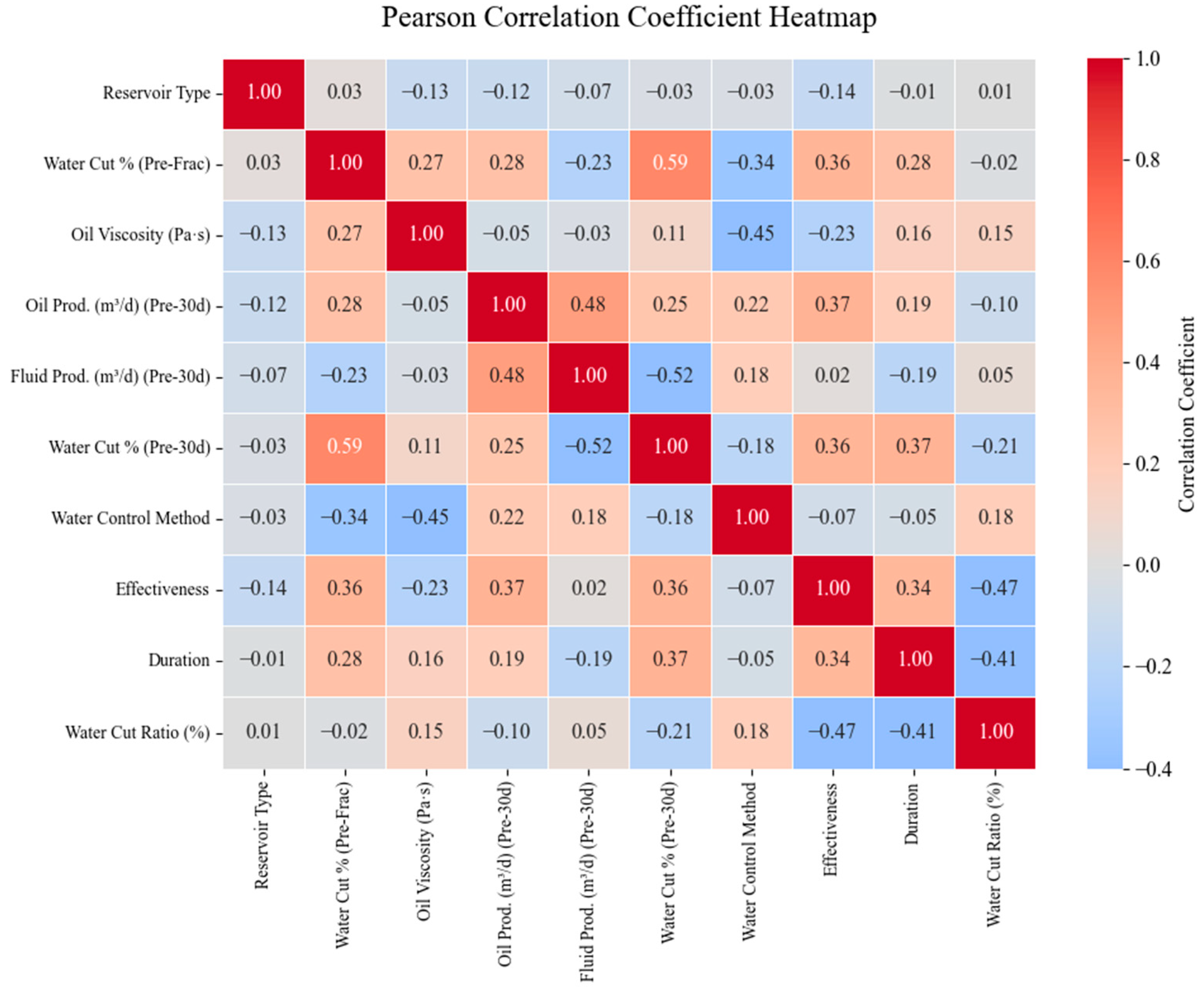
Based on the Pearson correlation analysis derived from Figure 1 and Table 3, four indicators exhibit positive correlations with effectiveness, while three demonstrate negative correlations. Quantitatively, most coefficients fall within a weak range (|r| < 0.4). Reservoir type (r = −0.14), oil production per day in the 30 days before the measure (r = 0.37), and water control technology (r = −0.07) all show very weak correlations with effectiveness (|r| < 0.2). In contrast, the oilfield’s comprehensive water cut percentage during the measure (r = 0.36), formation crude oil viscosity (r = −0.23), and the 30-day pre-measure water cut percentage (r = 0.36) exhibit relatively stronger—though still weak—correlations, with |r| values in the 0.23–0.36 range. Among all variables, the comprehensive water cut percentage, daily oil production, and pre-measure water cut percentage show the highest correlations with effectiveness.
For effective duration, four indicators show positive correlations and three show negative correlations. Five factors—including reservoir type (r = −0.01), oil viscosity (r = 0.16), daily oil production (r = 0.19), and water control method (r = −0.05)—exhibit very weak associations (|r| ≤ 0.2). The comprehensive water cut percentage (r = 0.28) and the 30-day pre-measure water cut percentage (r = 0.37) again show relatively stronger correlations, with |r| approaching 0.3. These two indicators therefore exhibit the strongest association with effective duration.
For water-cut-percentage comparison, four parameters show positive correlations and three show negative correlations. Most indicators fall within |r| < 0.2—for example, reservoir type (r = 0.01), oil viscosity (r = 0.15), daily oil production (r = −0.10), and water control method (r = 0.18). The only variable exceeding |r| = 0.2 is the 30-day pre-measure water cut percentage (r = −0.21), making it the indicator most strongly associated with the change in water cut after treatment.
Overall, Pearson correlation analysis indicates that the oilfield’s comprehensive water cut percentage (|r| = 0.28–0.36), formation crude oil viscosity (|r| = 0.15–0.23), and the 30-day pre-measure water cut percentage (|r| = 0.21–0.37) consistently exhibit the largest correlations with effectiveness, effective duration, and water-cut improvement.
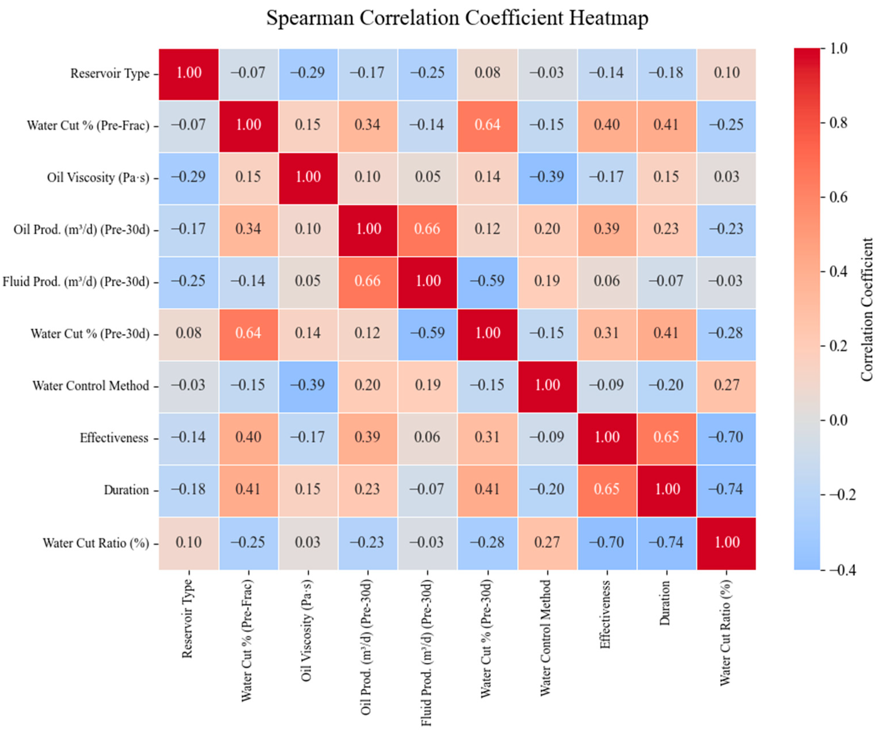
By studying the Spearman coefficients (Figure 2), several quantitative differences from the Pearson results can be observed. For example, the 30-day pre-measure water-cut percentage shows a higher monotonic correlation with effectiveness (rs = 0.31), duration (rs = 0.41), and water-cut ratio (rs = −0.28) compared with its Pearson values (0.36, 0.37, −0.21). Likewise, the water-cut percentage before fracturing exhibits stronger Spearman correlations with effectiveness and duration (rs = 0.40 and 0.41) than the corresponding Pearson values (0.36 and 0.28). Daily oil production 30 days before the measure also shows moderate monotonic correlations (rs = 0.39 with effectiveness; rs = 0.23 with duration), slightly higher than in Pearson analysis. In contrast, reservoir type continuously shows negligible monotonic correlation (|rs| ≤ 0.18).
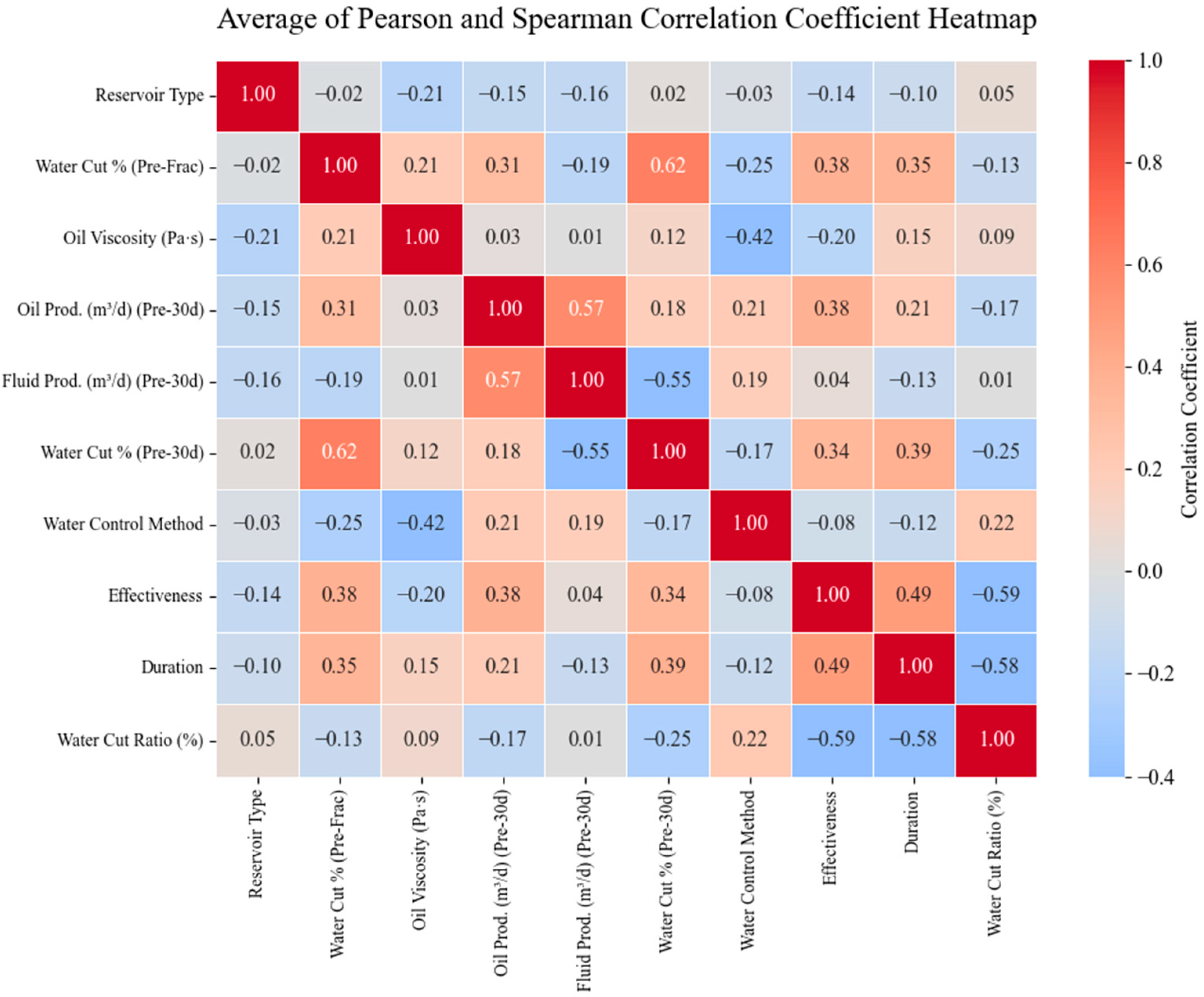
After averaging the Pearson and Spearman coefficients (Figure 3), the major influencing factors remain consistent, but the correlation magnitudes become smoother. The oilfield’s comprehensive water-cut percentage shows an averaged correlation of 0.38 with effectiveness and 0.35–0.39 with duration. The 30-day pre-measure water-cut percentage exhibits averaged correlations of 0.34 (effectiveness) and 0.39 (duration). Oil viscosity remains weakly associated (average |r| ≈ 0.12–0.21), while reservoir type and water control technology show very weak correlations (average |r| < 0.12). Overall, comprehensive water-cut percentage (average |r| = 0.35–0.38), daily oil production (average r = 0.21–0.38), and 30-day pre-measure water-cut percentage (average |r| = 0.34–0.39) demonstrate the strongest correlations with effectiveness and duration, consistent with the Pearson results, though still within the weak-to-moderate range.
For the correlation with effective duration, 4 indicators show a positive correlation, while 3 indicators show a negative correlation. Based on the quantitative Spearman results in Figure 2, the absolute correlation coefficients of reservoir type (|rs| = 0.18), formation crude oil viscosity (|rs| = 0.15), daily oil production in the 30 days before the measure (|rs| = 0.23), and water control technology (|rs| = 0.20) all fall within the 0–0.2 range in the averaged heatmap (Figure 3), indicating very weak correlations. In contrast, the three indicators—comprehensive water cut percentage of the oilfield during the measure (average |r| ≈ 0.35), daily liquid production during the 30-day pre-measure period (average |r| ≈ 0.13–0.19), and water cut percentage during the 30-day pre-measure period (average |r| ≈ 0.39)—show absolute correlation coefficients in the 0.2–0.4 interval, indicating weak correlations. Overall, the oilfield’s comprehensive water cut percentage at the time of measure implementation (rs = 0.41) and the 30-day pre-measure water cut percentage (rs = 0.41) exhibit the strongest associations with effective duration.
For the correlation with water cut percentage comparison, 4 indicators show a positive correlation, while 3 indicators show a negative correlation. According to the heatmap data, reservoir type (|r| = 0.05–0.10), comprehensive water cut percentage of the oilfield during the measure (|r| = 0.02–0.13), formation crude oil viscosity (|r| = 0.03–0.09), oil production per day in the 30 days before the measure (|r| = 0.10–0.17), and daily liquid production in the 30 days before the measure (|r| = 0.01–0.03) all show very weak correlations (0–0.2). Water cut percentage in the 30 days before the measure shows a stronger negative correlation with the water cut percentage comparison (Pearson r = −0.21; Spearman rs = −0.28; average |r| ≈ 0.25–0.28), while water control technology also shows weak correlation (average |r| = 0.22). Overall, the 30-day pre-measure water cut percentage and water control technology exhibit the strongest correlations with the water cut percentage comparison.
Through the combined Pearson and Spearman correlation analysis, the three indicators—comprehensive water cut percentage of the oilfield during the measure (average |r| ≈ 0.35–0.38), oil production per day in the 30 days before the measure (average |r| ≈ 0.21–0.38), and water cut percentage in the 30 days before the measure (average |r| ≈ 0.34–0.39)—show the strongest overall correlations with measure effectiveness (including effectiveness, effective duration, and water cut percentage comparison). Among these, the effectiveness is mainly influenced by the oilfield’s comprehensive water cut percentage during the measure (r = 0.36; rs = 0.40), daily oil production during the 30-day pre-measure period (r = 0.37; rs = 0.39), and the 30-day pre-measure water cut percentage (r = 0.36; rs = 0.31). The effective duration is most significantly correlated with the oilfield’s comprehensive water cut percentage during the measure (rs = 0.41) and the 30-day pre-measure water cut percentage (rs = 0.41). The 30-day pre-measure water cut percentage is the core influencing factor for the water cut percentage comparison (r = –0.21; rs = −0.28). Additionally, water control technology shows weak correlations (average |r| ≈ 0.18–0.22). Other indicators (such as reservoir type, oil viscosity, and daily liquid production) generally exhibit very weak correlations (|r| < 0.20).

5.2. Analysis of Measure Effectiveness in Different Reservoir Types

The differences in water invasion mechanisms between edge water reservoirs and bottom water reservoirs are key factors determining the effectiveness of water control measures. They each have distinct water invasion modes and water distribution, which leads to differentiated water control requirements.
In edge water reservoirs, water is mainly distributed on the sides of the reservoir, and the water invasion process typically progresses laterally. Because the water is located at the sides of the reservoir, the invasion speed is relatively slow and uniform [23]. Water control measures usually include profile control and chemical water shutoff technologies, which can effectively seal high-permeability streaks, thus delaying the water invasion speed and effectively controlling water expansion. By accurately identifying high-permeability zones and performing targeted sealing, water invasion in edge water reservoirs can remain relatively stable, and overall water flooding conditions are more controllable [24].
In contrast, for bottom water reservoirs, water is mainly located at the bottom of the reservoir, and the water invasion process is primarily characterized by vertical conical advancement. The vertical cone-shaped rise in water makes the invasion process more concentrated and rapid, easily influenced by production pressure differences, resulting in the formation of a water cone. To effectively control water, precise sealing of the bottom water rise channels near the wellbore is necessary, which requires higher technical demands. The sealing effect is often less stable compared to edge water reservoirs [28]. Therefore, bottom water reservoirs face higher technical challenges in water control.
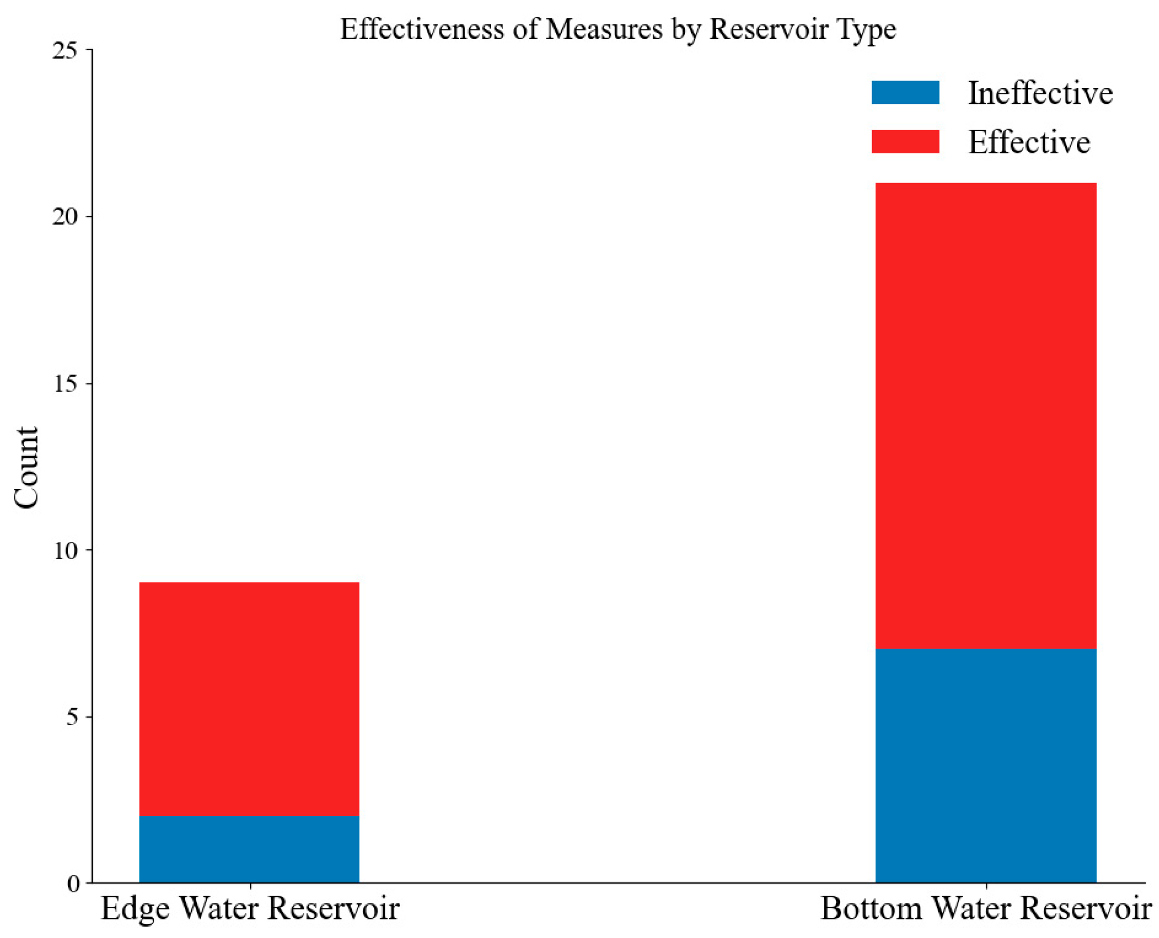
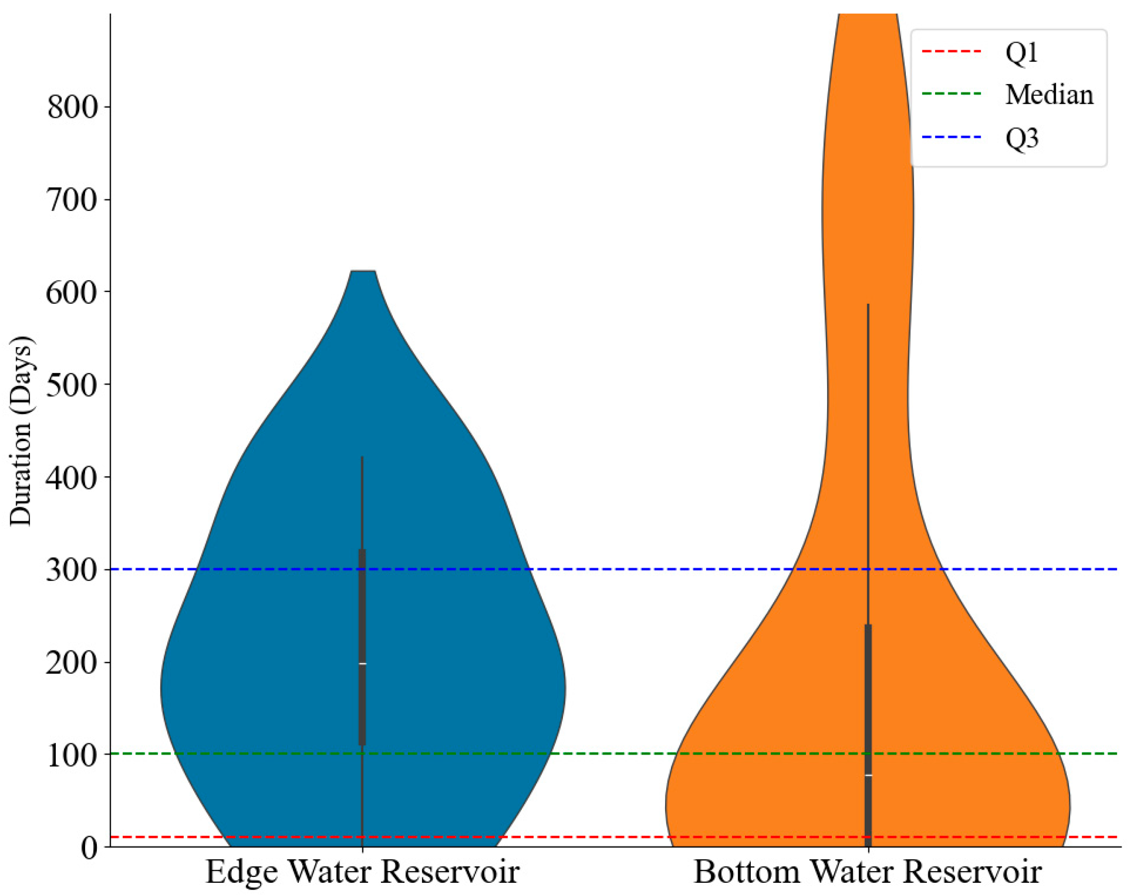
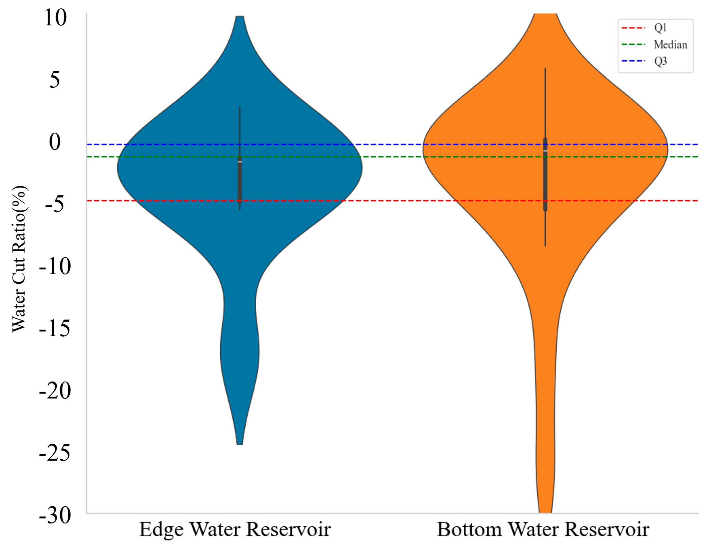
Through empirical analysis of the sample data, the comparison of water control measures for the two reservoir types was plotted as violin plots (Figure 4, Figure 5 and Figure 6), and the differences in water control effectiveness were analyzed.
As shown in Figure 4, in terms of effectiveness, bottom water reservoirs have a higher proportion of ineffective wells, approximately 25%, whereas edge water reservoirs have a 15% proportion of ineffective wells. The proportion of effective wells in bottom water reservoirs is lower, and some wells quickly become ineffective after showing results. This is closely related to the “re-cone” phenomenon, indicating that the water control measures in bottom water reservoirs are less stable than in edge water reservoirs, and the risk of ineffective wells is higher.
As shown in Figure 5, the duration of water control measures in edge water reservoirs is significantly longer than in bottom water reservoirs. The median effective duration for edge water reservoirs is concentrated between 400 and 600 days, while the effective duration for bottom water reservoirs is mainly concentrated below 200 days. More short-term duration outliers (<200 days) are observed in bottom water reservoirs, indicating that the water control effect in bottom water reservoirs is less stable and that the re-cone phenomenon is more common.
As shown in Figure 6, in terms of water cut percentage reduction, the distribution of the water cut percentage comparison in edge water and bottom water reservoirs shows some similarity, with the median concentrated between −10% and 0%, suggesting that both types of reservoirs can reduce the water cut percentage to some extent. However, the distribution range of water cut percentage in bottom water reservoirs is more dispersed, reflecting the higher volatility in the effectiveness of water control measures, which are less stable than in edge water reservoirs.
From the violin plots and data analysis results, it can be seen that the water control measures in edge water reservoirs are relatively stable. The effective duration of these measures is longer, with the median being more than 30% higher than in bottom water reservoirs. The proportion of ineffective wells is also lower. Overall, the water control effect in edge water reservoirs is more stable and carries a lower risk. In contrast, bottom water reservoirs are influenced by the water cone phenomenon, making water control measures more likely to experience re-cone formation, resulting in a shortened effective duration and significantly increased risk of ineffective wells. The heterogeneity and dynamic changes in the water cone in bottom water reservoirs are the fundamental causes of the volatility in water control effectiveness. Due to the strong heterogeneity of the water invasion process in bottom water reservoirs, the effectiveness of water control measures varies greatly, and significant differences are observed between different wells. As a result, the violin plot for bottom water reservoirs displays a “flat and wide” distribution. In edge water reservoirs, however, the water invasion path is relatively predictable, making the effectiveness of water control measures more consistent, with data distributions being relatively concentrated and showing less volatility.
For bottom water reservoirs, priority should be given to precise targeted water shutoff technologies, such as smart gels and liquid flow diverters. These technologies can effectively inhibit the formation of water cones and delay the water invasion process by optimizing the production pressure difference. Additionally, bottom water reservoirs require highly accurate water control techniques, so special attention must be given to the precise sealing of bottom water rise channels near the wellbore. For edge water reservoirs, a focus on high-dose deep-profile control can be effective in extending the duration of water control measures by sealing the dominant water flow channels. Since the water invasion path in edge water reservoirs is more predictable, the deep-profile control strategy can effectively delay water invasion and reduce the risk of measure failure.

5.3. Analysis of the Effectiveness of Different Water Control Technologies

In the process of reservoir development, controlling water invasion is crucial. Different water control technologies can be used based on the characteristics of water invasion. Table 4 shows an analysis of the mechanisms, advantages, and limitations of nine different water control technologies to better select the appropriate technology for different reservoir conditions [29,30].
Each water control technology has its unique mechanism and application scope. The specific selection should be based on reservoir characteristics (such as water invasion type, reservoir heterogeneity, etc.) and practical engineering needs [31,32].
Based on sample data, the effectiveness of different water control technologies was compared, and an analysis of effectiveness indicators (including effectiveness, effective duration, and water cut percentage comparison) was performed.
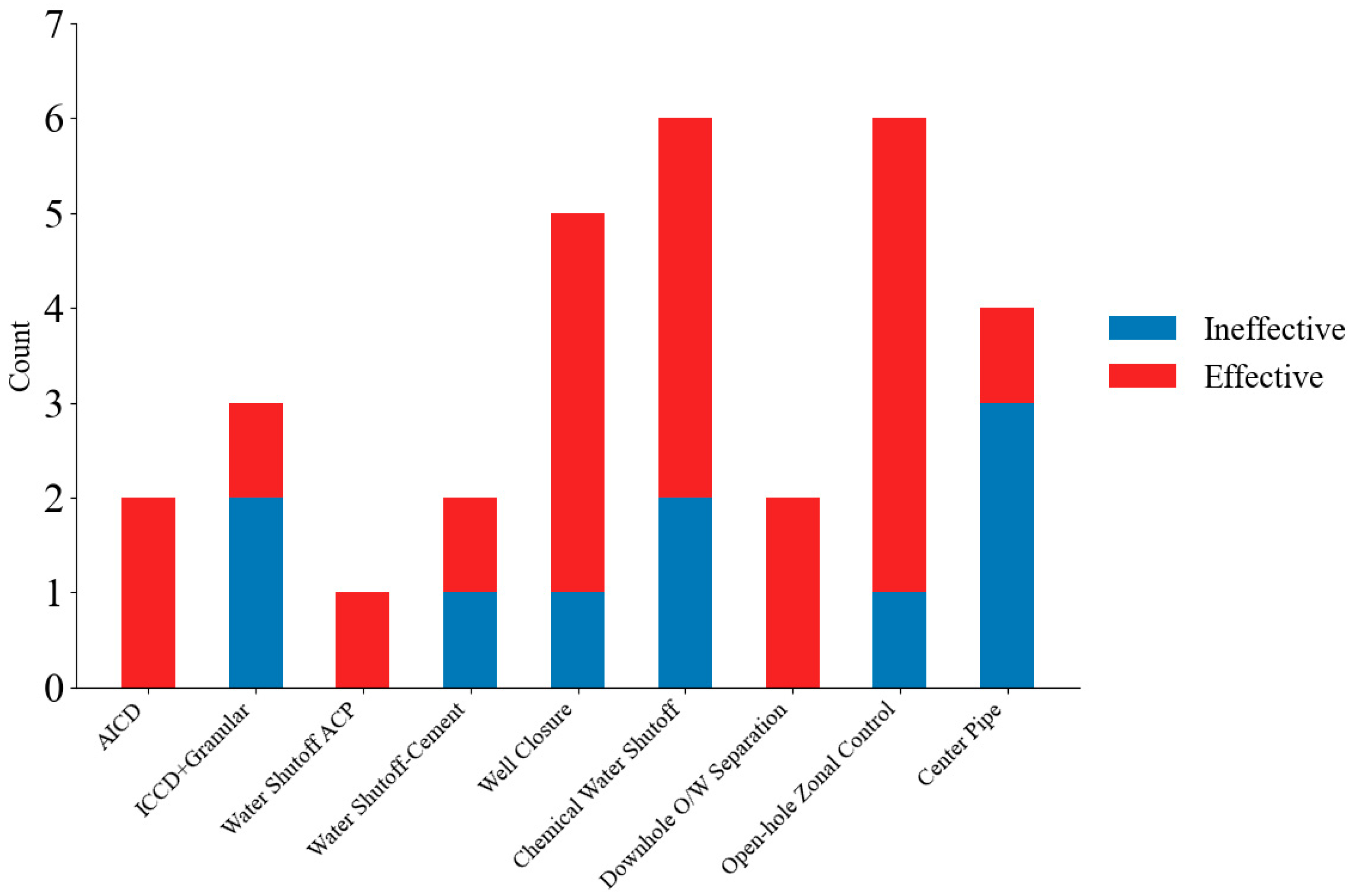
From the effectiveness data in Figure 7, it can be observed that the number of wells implementing shut-in pressure cone, openhole partition water control, and chemical water shutoff is the highest, accounting for 35%, and their effectiveness exceeds 60%, indicating that these technologies have a high potential for large-scale application. The effectiveness of AICD, water shutoff-ACP, and downhole oil-water separation is also high, all exceeding 75%, although the number of wells implementing these methods is lower. ICCD + particle filling and central pipe perform poorly, with more than 60% of ineffective wells, which is related to the high failure rates of equipment and high maintenance costs.
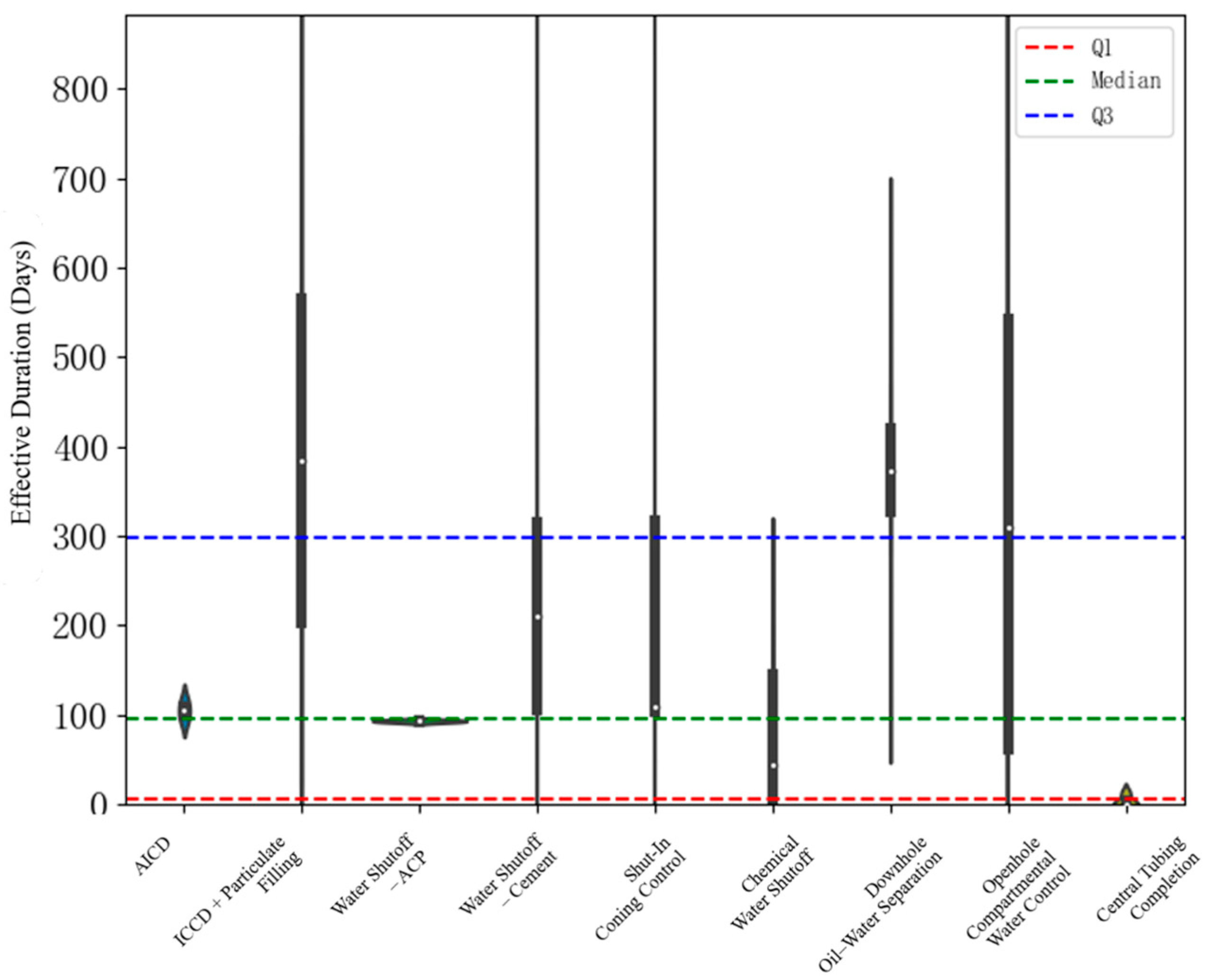
As shown in Figure 8, ICCD + particle filling has the longest effective duration, with a median value close to 400 days, demonstrating its advantage in long-term water control. Secondly, openhole partition water control also has a relatively long effective duration, with a median value of about 300 days. In contrast, AICD, water shutoff-ACP, chemical water shutoff, and central pipe have the shortest effective durations, all below 100 days, confirming that these methods are only suitable as temporary emergency measures.
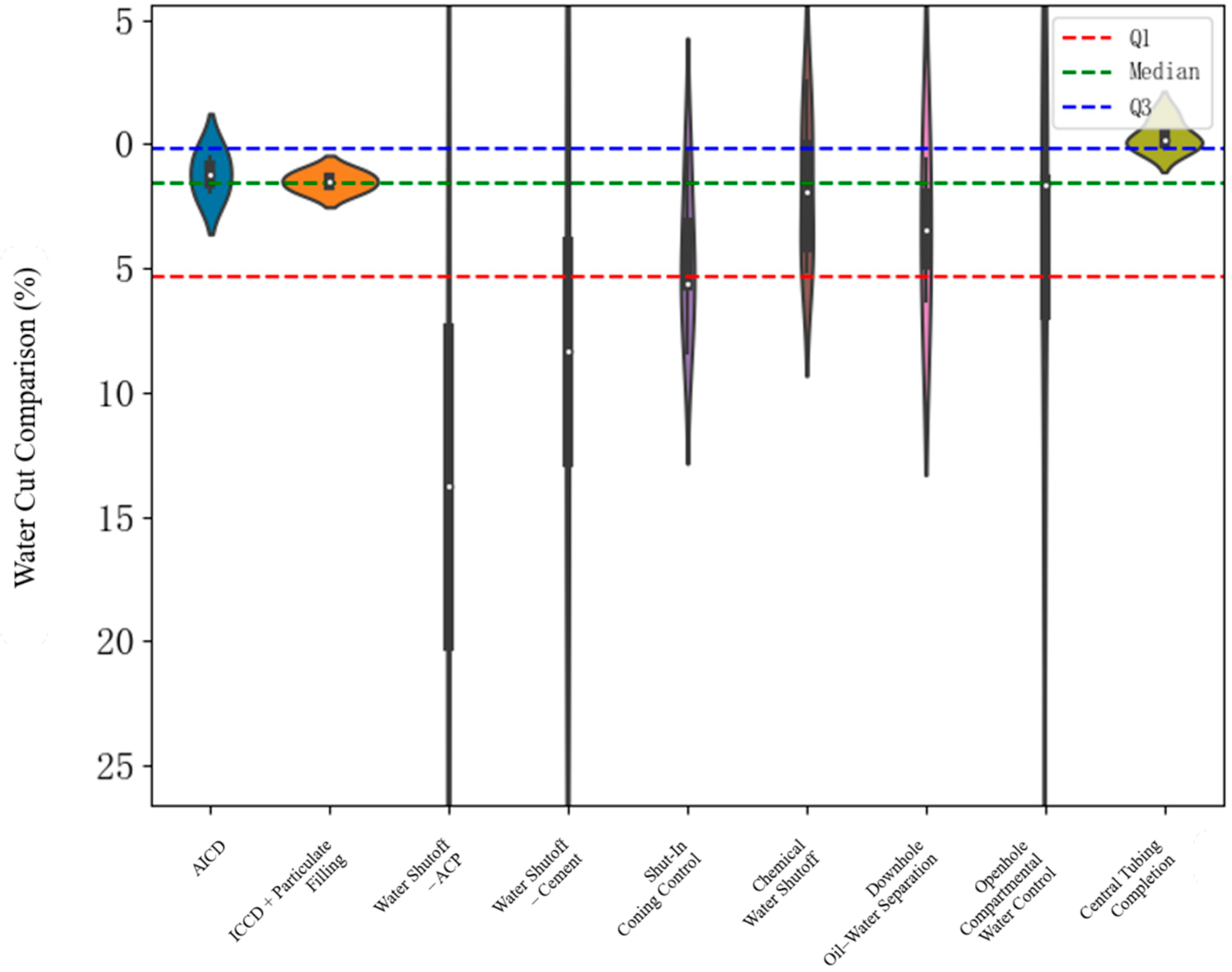
As shown in Figure 9, water shutoff-ACP and water shutoff-cement perform best in terms of water cut percentage reduction, with the median reduction for water shutoff-ACP ranging from −15% to −10%, and water shutoff-cement falling within this same range. Both data distributions are relatively concentrated, reflecting the stability of their effects. Chemical water shutoff and openhole partition water control have moderate reductions, around −10% to −5%. In contrast, shut-in pressure cone and central pipe have the smallest reductions, close to 0%, indicating that these two methods have weak effects and are ineffective in controlling water invasion.
Based on the above analysis, the effectiveness of various water control technologies can be classified, and optimization directions can be proposed. The strongly recommended technologies are: water shutoff-ACP and openhole partition water control. Water shutoff-ACP has the largest water cut percentage reduction (−15%) and the longest effective duration (>500 days), making it suitable for reservoirs with clearly defined high-permeability water channels, providing high stability and durability. Openhole partition water control is highly effective (>80%) and can be applied on a large scale, making it suitable for edge and bottom water reservoirs with openhole completions. The second-tier technologies are water shutoff-cement and chemical water shutoff. Water shutoff-cement has a significant water control effect in the short term but may fail over time, and it is recommended to enhance its performance with toughening agents to extend its effective duration. Chemical water shutoff has great potential, but a personalized formulation design for specific reservoirs is required to improve its stability and success rate. Shut-in pressure cone, central pipe, AICD, and ICCD + particle filling should be used with caution. Shut-in pressure cone and central pipe should only be used as emergency measures, with limited effects and not suitable for long-term application. AICD and ICCD + particle filling have small sample sizes and require further testing to verify their economic feasibility and applicability.
It should be noted that water shutoff-ACP and water shutoff-cement may cause damage to reservoir permeability, and it is recommended to optimize the toughness of the shutoff agents, such as adding flexible fibers, to reduce damage to the reservoir. The equipment stability of downhole oil–water separation is poor, with a high failure rate, so it is necessary to improve the equipment’s sand and scale resistance to ensure its long-term effectiveness. Openhole partition water control can be promoted on a large scale, but it has greater completion difficulty and higher costs, so it is recommended to use efficient completion tools to reduce overall costs and improve economic efficiency.

5.4. Canonical Correlation Analysis

Traditional bivariate correlation analyses can only assess the association between two single variables, failing to comprehensively capture the complex systemic nature of the factors influencing water control measures. The effectiveness of water control is the result of the combined action of multiple geological and dynamic production factors, and its evaluation involves multiple dimensions. Therefore, CCA is employed in this study to overcome this limitation.
As shown in Table 5, Table 6 and Table 7, based on sample data, two groups of variables were constructed: the independent variable group (reservoir parameters and production dynamics) and the dependent variable group (measure effectiveness), resulting in three pairs of canonical variables. The first pair passed the significance test (p = 0.047 < 0.05), with a canonical correlation of 0.619 (moderate correlation). The second pair (r = 0.492) and third pair (r = 0.323) did not pass the test (p > 0.05) and lack statistical significance.
Canonical variable for the independent variable group (U):
U = 0.227 × Reservoir Type − 0.575 × Field Average Water Cut During Measure + 0.397 × Reservoir Oil Viscosity − 0.590 × Production Liquid During the First 30 Days − 0.560 × Water Cut During the First 30 Days + 0.096 × Water Control Technology
Canonical variable for the dependent variable group (V):
V = −0.997 × Effectiveness − 0.276 × Effective Duration + 0.432 × Water Cut Comparison
Among the independent variables, the three indicators with the largest canonical loadings—daily liquid production during the first 30 days, field average water cut at the time of treatment, and water cut during the first 30 days—contribute most strongly to the canonical variable U. Water-control technology shows a comparatively minor contribution. For the dependent variable group, effectiveness dominates the canonical variable V, with a loading magnitude close to 1.
The first pair of canonical variables (U and V) captures the strongest linkage between geological/production characteristics and the effectiveness of water-control operations. The high loadings of pre-treatment water cut and early liquid production on U indicate that the severity of formation water invasion is the principal factor determining treatment outcomes. Meanwhile, V is mainly influenced by post-treatment water-cut reduction and effective duration, implying that the measurable response of water-control treatments is most sensitive to the initial level of water influx. This means that wells experiencing stronger pre-existing water invasion tend to exhibit more evident improvements after water-control interventions, whereas wells with relatively low initial water cut typically show limited enhancement. Therefore, the first canonical variable pair reflects the engineering relationship between water-invasion severity (U) and measure responsiveness (V), offering an interpretable basis for evaluating water-control potential under different reservoir and well conditions.

6. Water Control Measures Effect Prediction

The effectiveness of water control measures directly impacts the stable production and economic benefits of offshore oil fields. However, predicting the effectiveness of these measures is challenging due to the complex influence of factors such as reservoir geological characteristics, production dynamics, and process types. Based on the sensitivity analysis of key factors influencing the effectiveness of the measures in Section 3, a data-driven prediction model is constructed to achieve a quantitative prediction of the effectiveness of water control measures, providing support for measure optimization and decision-making.

6.1. Model Design

6.1.1. Model Input and Output

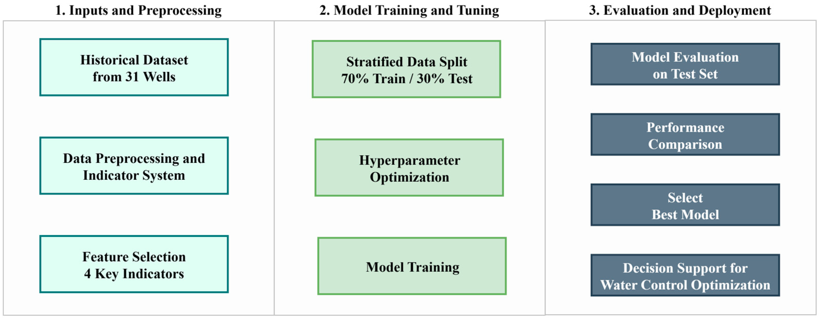
To effectively predict the effectiveness of water control measures, this study, building on the correlation analysis in Section 2, selected four key indicators most closely associated with effectiveness as model inputs: comprehensive water cut percentage of the oilfield during the measure, formation crude oil viscosity, daily liquid production 30 days before the measure and water cut percentage 30 days before the measure. These four characteristics together constitute a three-dimensional feature space encompassing both static geological information and recent dynamic production data. While the bivariate Pearson and Spearman analyses show a weak-to-moderate linear correlation for daily liquid production 30 days before the measure, the inclusion of this feature is justified by two primary factors: First, the Canonical Correlation Analysis identified it as a high-load component (−0.590) in the first canonical variable U1, indicating its strong systemic association with measure effectiveness 11. Second, from an engineering perspective, daily liquid production is a fundamental operational constraint, influencing both the technical feasibility and the economic scale of any water control operation, thus it must be retained in the final prediction system despite moderate individual correlation. The model’s prediction objective is a comprehensive evaluation of the measures after implementation, a typical binary classification problem. Therefore, the output is a binary label indicating whether the measures are “effective” or “ineffective.” The overall architecture of the model is shown in Figure 10.
The dataset is constructed based on samples from 31 historically treated wells and is partitioned into training and test sets in a 7:3 ratio to ensure the reliability of the model evaluation. Stratified sampling is used in the partitioning process to ensure that the ratio of “effective” to “ineffective” samples in the training and test sets remains consistent with that in the original dataset.

6.1.2. Prediction Algorithm Selection and Design

To compare the performance of different algorithms, this study uses three algorithms—Random Forest, Gradient Boosting, and Logistic Regression—to build the classification prediction model.

6.2. Model Construction and Validation

Based on the three classification algorithms, this study designed a prediction model that relies on four core indicators.
(1)
Model Training and Hyperparameter Optimization
To fully leverage the potential of each algorithm and avoid suboptimal results that might result from using default parameters, all models were optimized using cross-validation combined with grid search (GridSearchCV). Logistic regression primarily optimized the regularization parameter C; random forest optimized the number of trees (n_estimators) and depth (max_depth); and gradient boosting adjusted the learning rate (learning_rate), number of iterations, and tree depth. To achieve more stable and reliable performance evaluation, a 5-fold stratified cross-validation strategy was used. During the optimization process, all numerical features were normalized to eliminate the impact of dimensionality differences on model performance. AUC, accuracy, precision, recall, and F1-score were used as performance metrics.
(2)
Experimental Results and Analysis
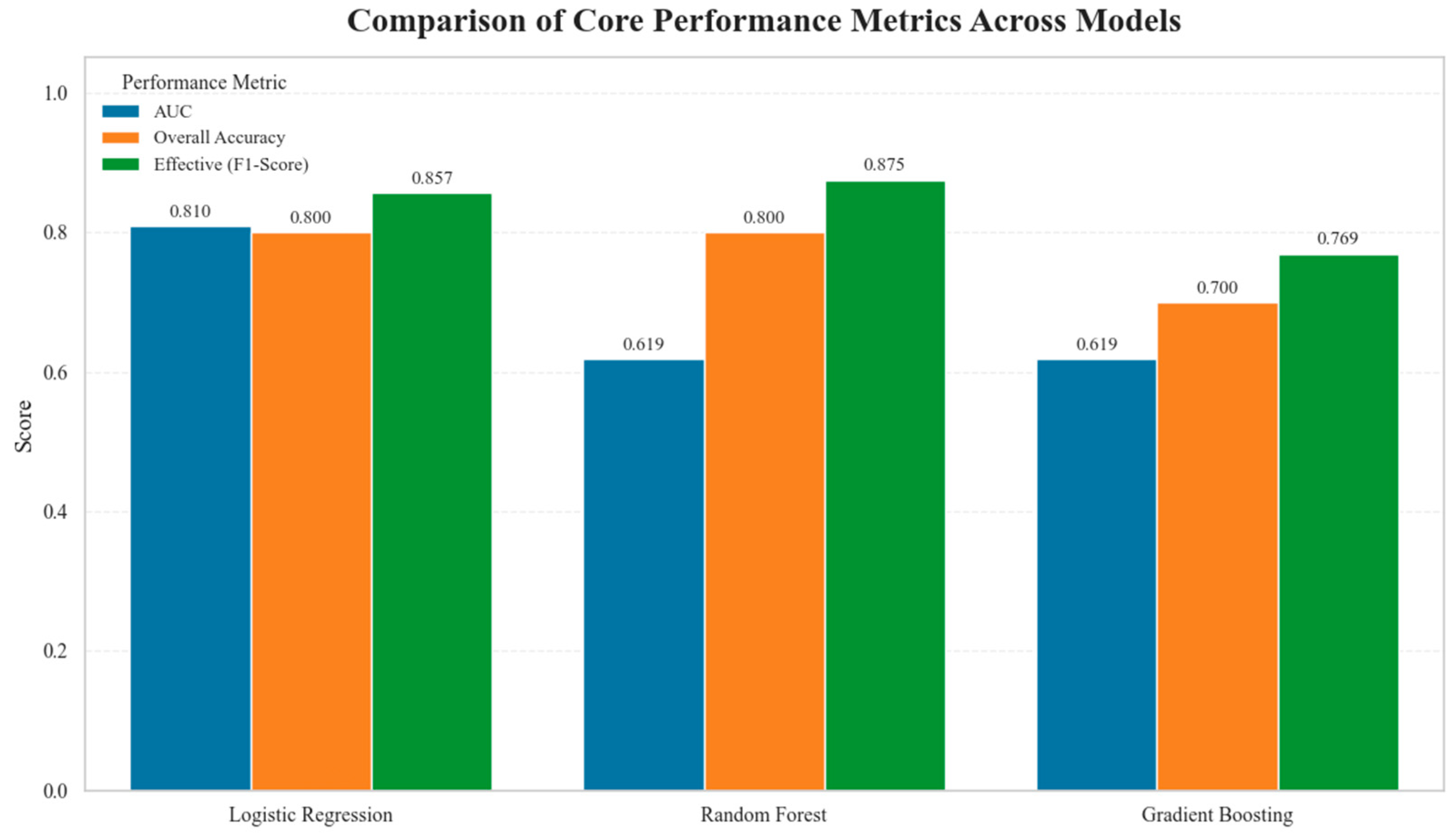
After parameter optimization, the performance of the three models on cross-validation and independent test sets is summarized in Table 8. As can be seen from the table, logistic regression has the highest cross-validation AUC (0.767) and the independent test set AUC reaches 0.81, which is the most robust overall. Although the accuracy of random forest is as high as 80%, its AUC is only 0.667, indicating that its classification probability distribution is not reliable enough. Gradient boosting has the weakest overall effect. It is noteworthy that while Random Forest and Gradient Boosting models theoretically possess stronger non-linear fitting capabilities, their suboptimal performance compared to Logistic Regression is primarily attributed to overfitting caused by the inherent small sample size (N = 31) of the dataset. Complex tree-based models tend to learn noise and irrelevant patterns present in sparse data, leading to low generalization ability as indicated by the poor AUC on the independent test set (0.667 for RF). For such scenarios, future strategies, such as increasing the regularization strength (for GB) or performing data augmentation (if feasible), are necessary to mitigate overfitting and improve reliability.
To more intuitively compare the performance of each model, Figure 11 shows their performance on core metrics. A low AUC indicates that the random forest’s ability and confidence in distinguishing “valid” from “invalid” samples is weak. In contrast, the high AUC value of logistic regression demonstrates its stronger discriminative ability. Random forest and gradient boosting, two theoretically more powerful models, performed poorly under the current small sample conditions.
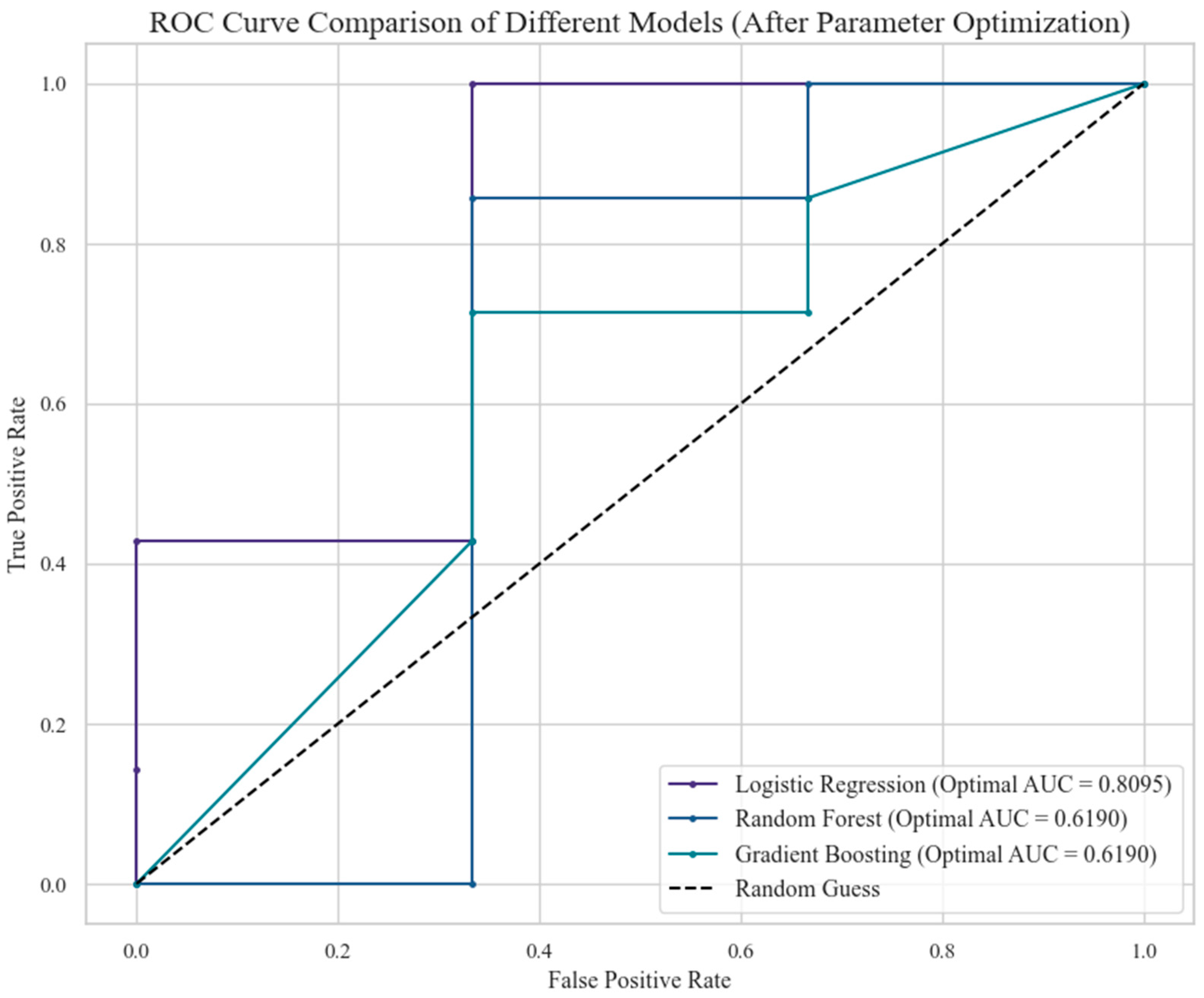
For the current task, a relatively simple linear model is sufficient to capture the primary relationship between the four key features and the effectiveness of the intervention. Although random forest achieved the same 80.00% accuracy as logistic regression on the test set, its area under the curve (AUC) was significantly lower, highlighting the limitations of evaluating models based solely on accuracy. As the gold standard for measuring a classifier’s comprehensive ranking and discrimination capabilities, AUC more accurately reflects a model’s generalization performance. To visually compare the various models’ abilities to distinguish between “effective” and “ineffective” samples, Figure 12 shows their receiver operating characteristic (ROC) curves on the test set. As can be seen, the ROC curve for logistic regression completely encompasses the curves for random forest and gradient boosting, demonstrating its strongest discriminative ability at all possible thresholds. This further confirms that, under the current small sample size conditions, the simpler logistic regression model can more stably capture the relationship between key features and the predicted target, avoiding the overfitting problem that can occur with more complex models.
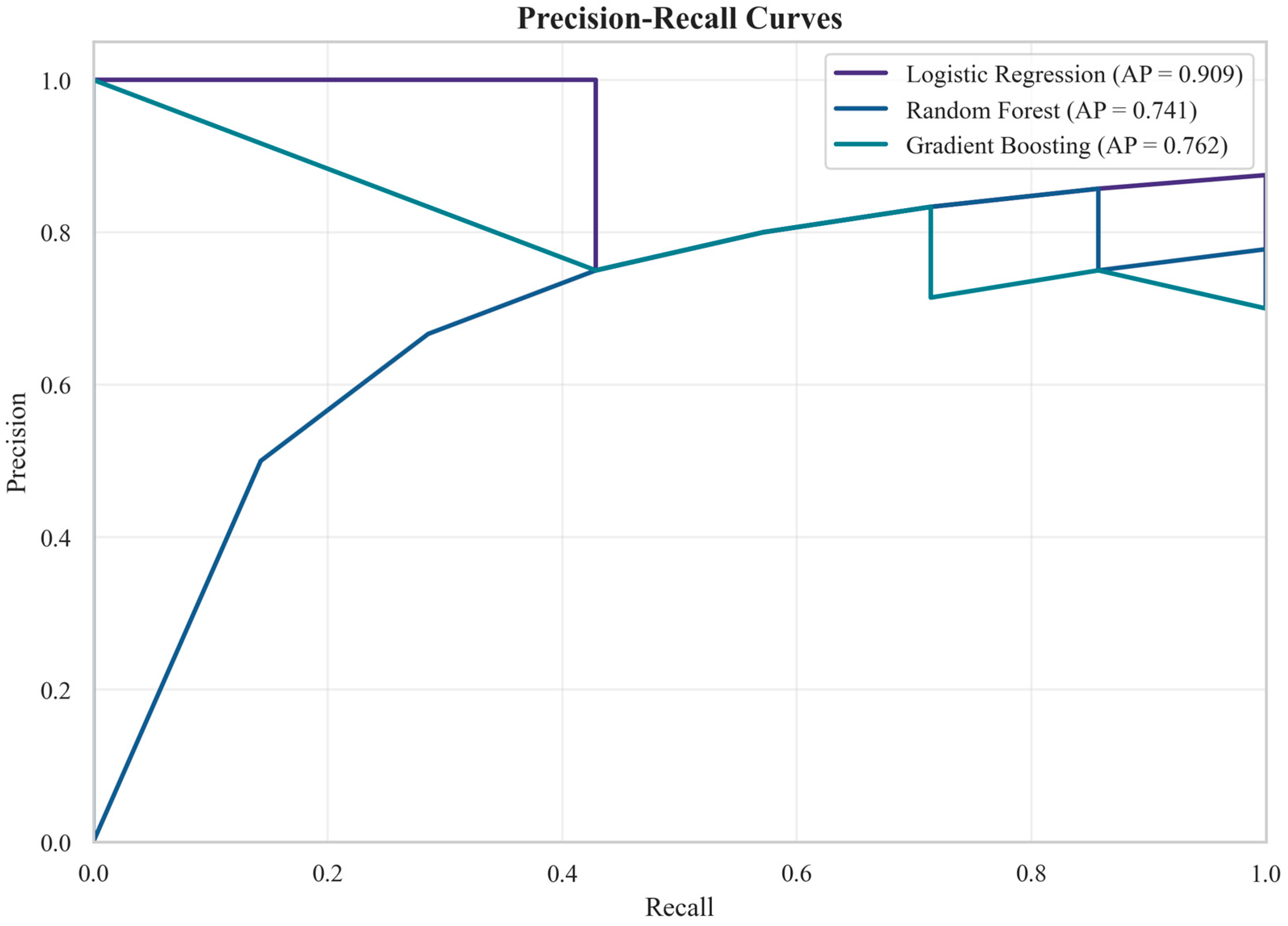
In addition to the ROC analysis, the precision–recall (P–R) curves provide further insight into the stability of the models under varying decision thresholds. Unlike ROC curves, which emphasize overall discrimination ability, P–R curves focus on the balance between the accuracy of positive predictions (precision) and the completeness of positive detection (recall).
As shown in Figure 13, the logistic regression model maintains consistently high precision even as recall increases, yielding the highest average precision (AP = 0.909). This indicates that the model can reliably identify effective cases while minimizing false positives. In contrast, random forest (AP = 0.741) and gradient boosting (AP = 0.762) display greater fluctuations in precision as recall rises, suggesting sensitivity to threshold changes and potential instability when class distributions are unbalanced.
These results highlight that, under small-sample and low-dimensional conditions, the simpler logistic regression model achieves a more stable precision–recall trade-off, which aligns with its superior AUC performance. Hence, it can provide more trustworthy predictions for the effectiveness of water control measures across diverse operating thresholds.
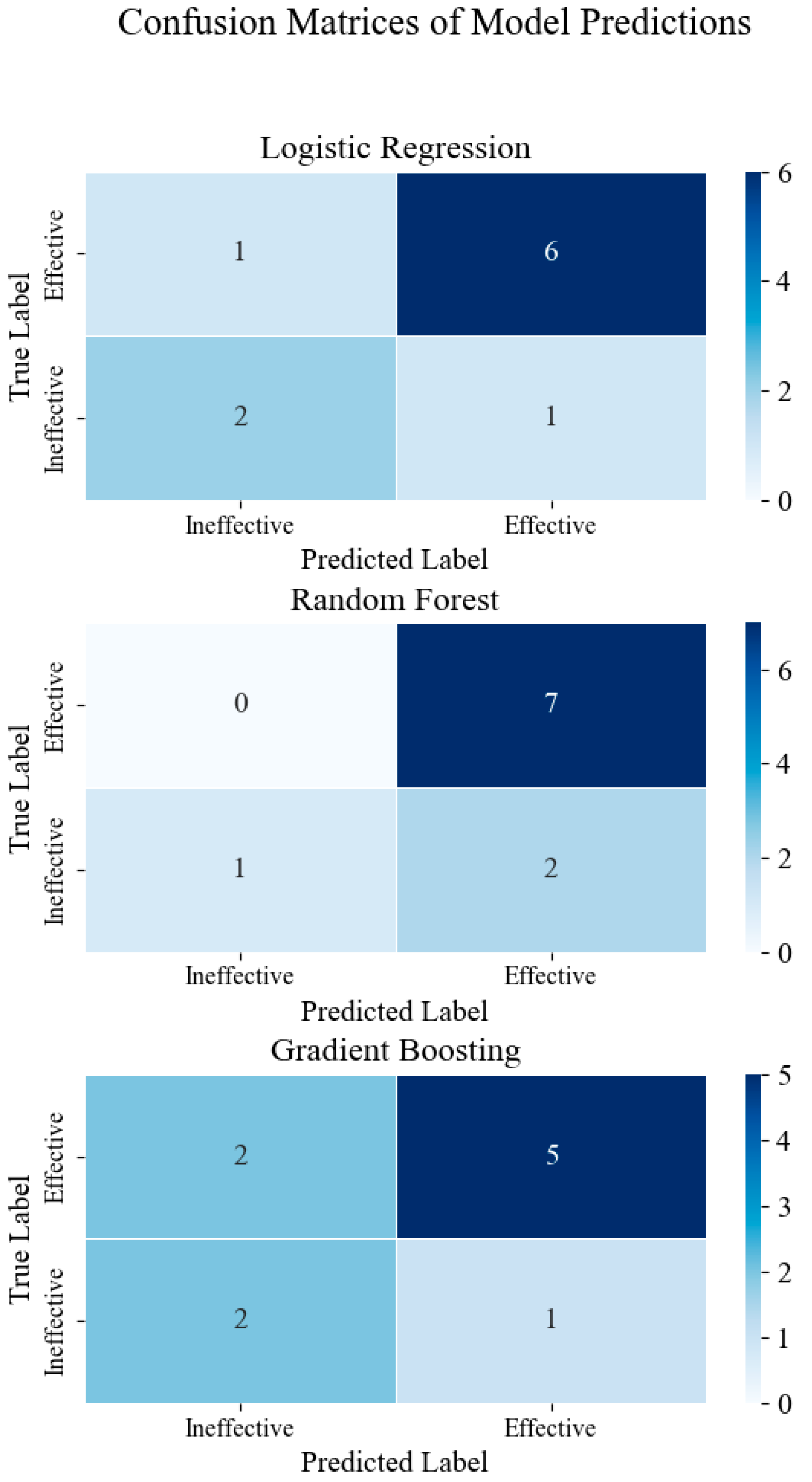
To further analyze the prediction behavior of each model, Figure 14 shows their confusion matrices on the test set. It can be seen that logistic regression achieves the best balance in correctly identifying “valid” and “invalid” samples.
Overall, logistic regression demonstrates the most robust and interpretable performance under small-sample and low-dimensional conditions. While random forest and gradient boosting theoretically possess higher representational power, their generalization ability is limited by data sparsity and feature redundancy. These results indicate that, for practical prediction of water control measure effectiveness, a linear model not only achieves stable accuracy but also provides valuable interpretability for engineering decision support.

7. Conclusions

This study systematically evaluates the implementation effects of water control measures and their key influencing factors through multi-dimensional statistical analysis and canonical correlation modeling. By combining reservoir characteristics and the adaptability of water control technologies, the following conclusions are drawn:
Water cut percentage is the core indicator affecting water control effectiveness. The study shows that comprehensive water cut percentage of the oilfield during the measure, water cut percentage 30 days before the measure, and daily liquid production 30 days before the measure are significantly correlated with the effectiveness of the measures.
The effectiveness duration of water control measures for edge water reservoirs is approximately 30% longer than for bottom water reservoirs, with a 10% lower ineffective well proportion. The primary reason for this difference is that water invasion in edge water reservoirs usually progresses laterally and is easier to control, while bottom water reservoirs are influenced by vertical water cones, making control more difficult.
Canonical correlation analysis reveals a moderate and significant correlation (ρ > 0.6) between reservoir production dynamics and water control measure effectiveness. Among these, the measure effectiveness is the core variable in the effectiveness response, indicating that the timeliness and stability of effectiveness play a crucial role in the success rate of water control.
The comparative analysis demonstrates that Logistic Regression is the best-performing model, yielding the highest performance with an AUC of 0.81 on both cross-validation and the independent test set. By contrast, Random Forest and Gradient Boosting show weaker performance under small-sample conditions, with unstable AUC values and lower robustness. These findings suggest that simpler linear models may provide more reliable diagnostic power than complex ensemble methods when data availability is limited.

Author Contributions

Conceptualization, F.L. and Q.L.; methodology, F.L.; software, F.L. and X.W.; validation, F.L.; formal analysis, F.L.; investigation, F.L.; resources, Y.H.; data curation, F.L. and X.W.; writing—original draft preparation, F.L.; writing—review and editing, C.Z.; visualization, C.Z.; funding acquisition, Q.L. All authors have read and agreed to the published version of the manuscript.

Funding

Project supported by the National Science and Technology Major Project of the Ministry of Science and Technology of China (No. 2024ZD1403800).

Data Availability Statement

Dataset available on request from the author.

Conflicts of Interest

Authors Fenghui Li and Yingxu He were employed by Caofeidian Operation Company, CNOOC (China) Co., Ltd. Authors Qiang Lu and Chunfeng Zheng were employed by CNOOC Energy Technology & Services Limited Key Laboratory for Enhanced Oil Recovery and CNOOC EnerTech-Drilling & Production Co. The remaining authors declare that the research was conducted in the absence of any commercial or financial relationships that could be construed as a potential conflict of interest.

References

  1. Seright, R.; Brattekas, B. Water shutoff and conformance improvement: An introduction. Pet. Sci. 2021, 18, 450–478. [Google Scholar] [CrossRef] [Scilit]
  2. Sun, X.; Bai, B. Comprehensive review of water shutoff methods for horizontal wells. Pet. Explor. Dev. 2017, 44, 1022–1029. [Google Scholar] [CrossRef] [Scilit]
  3. Bai, B.; Zhou, J.; Yin, M. A comprehensive review of polyacrylamide polymer gels for conformance control. Pet. Explor. Dev. 2015, 42, 525–532. [Google Scholar] [CrossRef] [Scilit]
  4. Okon, A.N.; Appah, D.; Akpabio, J.U. Water Coning Prediction Review and Control: Developing an Integrated Approach. J. Sci. Res. Rep. 2017, 14, 1–24. [Google Scholar] [CrossRef] [Scilit]
  5. Taha, A.; Amani, M. Overview of Water Shutoff Operations in Oil and Gas Wells; Chemical and Mechanical Solutions. ChemEngineering 2019, 3, 51. [Google Scholar] [CrossRef] [Scilit]
  6. Qu, J.; Wang, P.; You, Q.; Zhao, G.; Sun, Y.; Liu, Y. Soft Movable Polymer Gel for Controlling Water Coning of Horizontal Well in Offshore Heavy Oil Cold Production. Gels 2022, 8, 352. [Google Scholar] [CrossRef] [Scilit]
  7. Seifi, F.; Haghighat, F.; Nikravesh, H.; Kazemzadeh, Y.; Azin, R.; Osfouri, S. Using new chemical methods to control water production in oil reservoirs: Comparison of mechanical and chemical methods. J. Pet. Explor. Prod. Technol. 2024, 14, 2617–2655. [Google Scholar] [CrossRef] [Scilit]
  8. Das, H.S.; Das, D.K.; Maity, S.K.; Khatua, D.; Gupta, G.K.; Jalgham, R.T.T.; Akitsu, T.; Kaushik, A.; Bhattacharyya, S.; Roymahapatra, G. Challenges of Gel Treatment Application for Conformance Control. Eng. Sci. 2024, 31, 1238. [Google Scholar] [CrossRef] [Scilit]
  9. Ahmed, A.A.; Saaid, I.M.; Sambo, C.; Shafian, S.R.M.; Hamza, M.F. Experimental investigation and numerical simulation of relative permeability modifiers during water shut-off. Geoenergy Sci. Eng. 2023, 230, 212095. [Google Scholar] [CrossRef] [Scilit]
  10. Hu, J.; Zhang, G.; Jiang, P.; Wang, X.; Wang, L.; Pei, H. A new method of water control for horizontal wells in heavy oil reservoirs. Geoenergy Sci. Eng. 2023, 222, 211391. [Google Scholar] [CrossRef] [Scilit]
  11. Liu, X.; Song, H.; Zhao, L.; Zheng, Y.; Yang, N.; Qiu, D. Study on Optimal Water Control Methods for Horizontal Wells in Bottom Water Clastic Rock Reservoir. Fluid Dyn. Mater. Process. 2024, 20, 2377. [Google Scholar] [CrossRef] [Scilit]
  12. Zou, Q.; Chen, Z.; Cheng, Z.; Liang, Y.; Xu, W.; Wen, P.; Zhang, B.; Liu, H.; Kong, F. Evaluation and intelligent deployment of coal and coalbed methane coupling coordinated exploitation based on Bayesian network and cuckoo search. Int. J. Min. Sci. Technol. 2022, 32, 1315–1328. [Google Scholar] [CrossRef] [Scilit]
  13. Wang, X.; He, Y.; Li, F.; Wang, Z.; Dou, X.; Xu, H.; Fu, L. A working condition diagnosis model of sucker rod pumping wells based on deep learning. SPE Prod. Oper. 2021, 36, 317–326. [Google Scholar] [CrossRef] [Scilit]
  14. Liu, Y.; Zhang, Y.; Xue, B.; Lu, Y.; Wang, J.; Zhou, J.; Liu, T. Application of Binary Compound Water Control Technology in The Development of Horizontal Wells in Offshore Oil Fields. IOP Conf. Ser. Earth Environ. Sci. 2019, 384, 012111. [Google Scholar] [CrossRef] [Scilit]
  15. Wang, D.; Li, Y.; Ma, L.; Yu, F.; Liu, S.; Qi, T.; Jiang, S. Evaluation of the Effectiveness and Adaptability of a Composite Water Control Process for Horizontal Wells in Deepwater Gas Reservoirs. Front. Earth Sci. 2022, 10, 906949. [Google Scholar] [CrossRef] [Scilit]
  16. Mathiesen, V.; Aakre, H.; Werswick, B.; Elseth, G. The Autonomous RCP Valve—New Technology for Inflow Control in Horizontal Wells. In Proceedings of the SPE Offshore Europe Oil and Gas Conference and Exhibition, Aberdeen, UK, 6–8 September 2011. SPE-145737-MS. [Google Scholar] [CrossRef] [Scilit]
  17. Seright, R.S.; Lane, R.H.; Sydansk, R.D. A Strategy for Attacking Excess Water Production. SPE Prod. Facil. 2003, 18, 158–169. [Google Scholar] [CrossRef] [Scilit]
  18. Boyun, G.; Lee, R.L.-H. A Simple Approach to Optimization of Completion Interval in Oil/Water Coning Systems. SPE Reserv. Eng. 1993, 8, 249–255. [Google Scholar] [CrossRef] [Scilit]
  19. Wang, X.; Yu, W.; Xie, Y.; He, Y.; Xu, H.; Chu, X.; Li, C. Numerical Simulation of the Dynamic Behavior of Low Permeability Reservoirs Under Fracturing-Flooding Based on a Dual-Porous and Dual-Permeable Media Model. Energies 2024, 17, 6203. [Google Scholar] [CrossRef] [Scilit]
  20. Ahn, S.; Lee, K.; Choe, J.; Jeong, D. Numerical approach on production optimization of high water-cut well via advanced completion management using flow control valves. Pet. Explor. Prod. Technol 2023, 13, 1611–1625. [Google Scholar] [CrossRef] [Scilit]
  21. Obino, V.; Yadav, U. Application of polymer based nanocomposites for water shutoff—A review. Fuels 2021, 2, 304–322. [Google Scholar] [CrossRef] [Scilit]
  22. Xie, K.; Wu, Z.; Li, X.; Cao, W.; Yang, E.; Mei, J.; Gao, M.; Yuan, S. A review of research progress of in situ polyacrylamide gel for profile control and water plugging. Phys. Fluids 2025, 37, 091303. [Google Scholar] [CrossRef] [Scilit]
  23. Gu, P. A Study on Listening Comprehension Anxiety in Chinese Junior Middle School Students Based on the Pearson Correlation Analysis. In Proceedings of the 2021 2nd International Conference on Artificial Intelligence Education (ICAIE), Dali, China, 18–20 June 2021; pp. 332–335. [Google Scholar] [CrossRef] [Scilit]
  24. Janse, R.J.; Hoekstra, T.; Jager, K.J.; Zoccali, C.; Tripepi, G.; Dekker, F.W.; van Diepen, M. Conducting correlation analysis: Important limitations and pitfalls. Clin. Kidney J. 2021, 14, 2332–2337. [Google Scholar] [CrossRef] [Scilit]
  25. Uurtio, V.; Monteiro, J.M.; Kandola, J.; Shawe-Taylor, J.; Fernandez-Reyes, D.; Rousu, J. A Tutorial on Canonical Correlation Methods. ACM Comput. Surv. 2017, 50, 1–33. [Google Scholar] [CrossRef] [Scilit]
  26. Nimon, K.; Henson, R.K.; Gates, M.S. Revisiting Interpretation of Canonical Correlation Analysis: A Tutorial and Demonstration of Canonical Commonality Analysis. Multivar. Behav. Res 2010, 45, 702–724. [Google Scholar] [CrossRef] [Scilit]
  27. Wang, X.; Rui, C.; Liu, H. Analysis of Sensitive Factors for Sidetrack Drilling in Water-Flooded Oil Reservoirs: Data Mining Based on Actual Field Data. Front. Energy Res. 2023, 11, 1250336. [Google Scholar] [CrossRef] [Scilit]
  28. Alfarge, D.K.; Wei, M.; Bai, B. Numerical simulation study of factors affecting relative permeability modification for water-shutoff treatments. Fuel 2017, 207, 226–239. [Google Scholar] [CrossRef] [Scilit]
  29. Bin Marta, E.S.; Hammouda, M.M.M.S.; Tantawy, M.A.; Khamis, M.A.; Wahba, A.M. Diagnosing and Controlling Excessive Water Production: State-of-the-Art Review. J. Pet. Min. Eng. 2024, 25, 9–25. [Google Scholar] [CrossRef] [Scilit]
  30. Hayavi, M.T.; Kalantariasl, A.; Malayeri, M.R. Application of polymeric relative permeability modifiers for water control purposes: Opportunities and challenges. Geoenergy Sci. Eng. 2023, 231, 212330. [Google Scholar] [CrossRef] [Scilit]
  31. Zhang, D.; Li, Y.; Zhang, Z.; Li, F.; Liu, H. Research and Practice on Implementing Segmented Production Technology of Horizontal Well during Extra-High Water Cut Stage with Bottom Water Reservoir. Processes 2024, 12, 1142. [Google Scholar] [CrossRef] [Scilit]
  32. Yang, Y.; Li, F.; Zhang, W.; Li, X.; Pei, B. The continuous pack-off technology: A novel water-control method and application to offshore horizontal wells of limestone reservoir. J. Pet. Sci. Eng. 2022, 211, 110137. [Google Scholar] [CrossRef] [Scilit]
Figure 1. Pearson correlation coefficient heatmap.
Processes 14 00088 g001
Figure 2. Spearman correlation coefficient heatmap.
Processes 14 00088 g002
Figure 3. Pearson Spearman correlation coefficient average heatmap.
Processes 14 00088 g003
Figure 4. Measure Effectiveness.
Processes 14 00088 g004
Figure 5. Effective Duration.
Processes 14 00088 g005
Figure 6. Water cut percentage Comparison.
Processes 14 00088 g006
Figure 7. Effectiveness of Measures.
Processes 14 00088 g007
Figure 8. Effective Duration of Measures.
Processes 14 00088 g008
Figure 9. Comparison of Water cut percentage Before and After Measures.
Processes 14 00088 g009
Figure 10. Overall Architecture of Data-Driven Prediction Workflow.
Processes 14 00088 g010
Figure 11. Comparison of core performance indicators of each model.
Processes 14 00088 g011
Figure 12. Comparison of ROC curves of different models.
Processes 14 00088 g012
Figure 13. Precision–Recall curves of different models.
Processes 14 00088 g013
Figure 14. Confusion Matrices of Model Predictions.
Processes 14 00088 g014
Table 1. Indicator System.
TypeIndicator NameIndicator Meaning
Reservoir Geological ParametersSand BodyRefers to the stratigraphic section composed of sand particles, typically having good porosity and permeability, which is the main reservoir for oil and gas storage./
Reservoir TypeThe classification of reservoirs based on the distribution of water within the reservoir, divided into edge water reservoirs and bottom water reservoirs./
Reservoir Crude Oil ViscosityThe resistance to flow of oil in the reservoir.mPa · s
Water Shutoff and Control MeasuresWater Shutoff TechnologiesAICD (Autonomous Inflow Control Device): An intelligent completion device that autonomously regulates flow resistance according to fluid properties, thereby improving inflow profile control.
ICCD + Particulate Filling: A fixed-choke inflow control device integrated into gravel-packed sand-control completions to enhance inflow regulation and delay water breakthrough.
Water Shutoff—ACP: A delayed crosslinked polymer-clay composite plugging agent designed to seal high-permeability water channels and improve shutoff effectiveness.
Water Shutoff—Cement: Application of oilwell cement slurry to seal water-producing intervals, providing low-cost isolation with high compressive strength.
Shut-in Coning: A pressure management technique that suppresses upward water cone development by periodically shutting in wells to reduce drawdown.
Chemical Water Shutoff: The use of chemical agents, such as polymers or gels, for selective plugging of water-bearing zones to enhance reservoir conformance.
Downhole Oil–Water Separation: Downhole centrifugal or gravity-based technology that separates oil and water within the wellbore, enabling water reinjection and independent oil production.
Openhole Compartmental Water Control: Deployment of expandable packers in open-hole horizontal sections to divide the borehole into multiple isolated compartments for targeted water control.
Central Tubing Completion: Installation of a small-diameter tubing inside the casing to create a dual annulus-tubing flow channel, reducing production pressure differences at low cost.
/
Production Data Before and After MeasuresDaily Liquid ProductionThe daily production of liquid (oil + water) of the well 30 days before and after the measure.m3/d
Daily Oil ProductionThe daily production of oil of the well 30 days before and after the measure.m3/d
Water Cut PercentageThe percentage proportion of water in the produced liquid on a daily basis.%
Comparison of Production Data Before and After MeasuresDaily Liquid Production ReductionThe decrease in daily liquid output after the water-shutoff measure compared to before the measure.m3/d
Daily Water Production ReductionThe decrease in daily water production after the water-shutoff measure compared to before the measure.m3/d
Water Cut Percentage ComparisonThe decrease in water cut after the water cut percentage measure compared to before.%
Daily Oil Increment (Industry Standard Method)Daily oil increase = Post-measure daily oil − Predicted pre-measure daily oil.m3/d
Daily Oil Increment (Net Water Cut Reduction Method)Daily oil increase = Post-measure daily liquid × (Pre-measure water cut percentage − Post-measure water cut percentage)/(1 − Post-measure water cut percentage).m3/d
Daily Oil Increment (Constant Liquid Production Method)Daily oil increase = Post-measure daily oil − [Pre-measure daily oil × (Post-measure daily liquid/Pre-measure daily liquid)].m3/d
Table 2. Sample Set.
Geological Development CharacteristicsWater Control MeasuresMeasure Effectiveness
Sand BodyWater Shutoff TechnologyEffectiveness situation
Formation Crude Oil Viscosity
Fieldwide comprehensive water cut (%) at the time of the measure
Reservoir Type (Edge Water/Bottom Water)Validity period
Daily Liquid Production 30 days Before Measure (m3/d)
Daily Oil Production 30 days Before Measure (m3/d)Water Cut Comparison
Water Cut 30 Days Before Measure (%)
Table 3. Classification and Evaluation of Pearson Correlation Coefficients.
Pearson Correlation CoefficientRelationship Between VariablesDegree of Correlation (Strength)
ρX, Y = 1Perfect Positive Linear CorrelationVery Strong
0.8 < ρX, Y < 1.0Strong Positive Linear CorrelationVery Strong
0.6 < ρX, Y < 0.8Positive Linear CorrelationStrong
0.4 < ρX, Y < 0.6Weak Positive Linear CorrelationModerate
0.2 < ρX, Y < 0.4Very Weak Positive Linear CorrelationWeak
0 < ρX, Y < 0.2Negligible Positive Linear CorrelationVery Weak or No Correlation
ρX, Y = 0Absence of a Linear RelationshipVery Weak or No Correlation
−0.2 < ρX, Y < 0Negligible Negative Linear CorrelationVery Weak or No Correlation
−0.4 < ρX, Y < −0.2Very Weak Negative Linear CorrelationWeak
−0.6 < ρX, Y < −0.4Weak Negative Linear CorrelationModerate
−0.8 < ρX, Y < −0.6Strong Negative Linear CorrelationStrong
−1.0 < ρX, Y < −0.8Very Strong Negative Linear CorrelationVery Strong
ρX, Y = −1Perfect Negative Linear CorrelationVery Strong
Table 4. Characteristics of Water Control Technologies.
Technology TypeMechanismAdvantagesLimitations
AICD (Autonomous Inflow Control Device)Adaptive inflow regulation based on fluid viscosity contrastPrecise autonomous water control, no surface intervention requiredStrongly dependent on reservoir fluid properties; relatively high cost
ICCD + Particulate FillingInflow control completion device combined with particulate packing to regulate inflow profileDelays water breakthrough; enhances flow stability in horizontal and multilateral wellsLimited applicability to specific well configurations
Water Shutoff—ACPPolymer gel-cement composite plugging agent that seals high-permeability channelsHigh mechanical strength; extended effective durationRisk of formation damage; potential impairment of reservoir permeability
Water Shutoff—CementCement-based plugging of water-bearing channelsLow cost; high compressive strengthBrittle; susceptible to cracking; poor adaptability to heterogeneous formations
Shut-In Coning ControlTemporary well shut-in to reduce drawdown and induce collapse of the water coneSimple operation; no direct costEffect is temporary; high risk of water re-coning after production resumption
Chemical Water ShutoffInjection of polymer gels or cross-linked agents for selective water pluggingEffective in complex pore networks; capable of deep reservoir penetrationRequires sophisticated formulation design; variable treatment success
Downhole Oil–Water SeparationDownhole centrifugal or membrane-based separation of oil and waterReal-time water control; preserves reservoir integrityHigh equipment failure rate; elevated maintenance cost
Openhole Compartmental Water ControlSegmented isolation and filling in openhole completions to suppress localized water breakthroughSuitable for uncased wells; broad applicability across heterogeneous reservoirsTechnically challenging completion; elevated operational risk
Central Tubing CompletionOptimized concentric tubing structure to regulate production pressure differentialsLow cost; straightforward implementationOnly mitigates apparent water cut percentage; does not eliminate fundamental water invasion mechanisms
Table 5. Canonical Loadings for Set 1.
Variable123
Reservoir Type0.227−0.038−0.154
Comprehensive Water Cut of the Oilfield During the Measure−0.5750.6060.032
Formation Crude Oil Viscosity (mPa · s)0.3970.527−0.265
Daily Liquid Production During the First 30 Days (m3/d)−0.5900.276−0.003
Daily Oil Production During the First 30 Days (m3/d)−0.059−0.2760.498
Water Cut During the First 30 Days (%)−0.5600.431−0.604
Water Control Technology0.0960.2070.422
Table 6. Canonical Loadings for Set 2.
Variable123
Effectiveness−0.9970.025−0.067
Effective Duration−0.2760.642−0.716
Water Cut Comparison (%)0.4320.4340.790
Table 7. Canonical Correlation.
Canonical VariableCorrelationEigenvalueWilks’ StatisticFNumerator dfDenominator dfSignificance p
10.6190.6220.4181.02721.00060.8510.047
20.4920.3200.6790.78412.00044.0000.663
30.3230.1160.8960.5355.00023.0000.747
Table 8. Performance comparison of different prediction models.
ModelCross-Validation Mean AUCIndependent Test Set AUCTest Set Accuracy
Logistic Regression0.76670.809580.00%
Random Forest0.70000.666780.00%
Gradient Boosting0.68330.619060.00%
Disclaimer/Publisher’s Note: The statements, opinions and data contained in all publications are solely those of the individual author(s) and contributor(s) and not of MDPI and/or the editor(s). MDPI and/or the editor(s) disclaim responsibility for any injury to people or property resulting from any ideas, methods, instructions or products referred to in the content.