Article

Automated Detection of Shading Faults in Photovoltaic Modules Using Convolutional Neural Networks and I–V Curves

by
Jesus A. Arenas-Prado
1,
Angel H. Rangel-Rodriguez
1,
Juan P. Amezquita-Sanchez
1,
David Granados-Lieberman
2,
Guillermo Tapia-Tinoco
3 and
Martin Valtierra-Rodriguez
1,*
1
ENAP-RG, CA-Sistemas Dinámicos y Control, Facultad de Ingeniería, Universidad Autónoma de Querétaro, Campus San Juan del Río, Río Moctezuma 249, Col. San Cayetano, San Juan del Río 76807, Querétaro, Mexico
2
ENAP-RG, Departamento de Ingeniería Electromecánica, Tecnológico Nacional de México, Instituto Tecnológico Superior de Irapuato, El Copal km 12.5, Irapuato 36821, Guanajuato, Mexico
3
ENAP-RG, Departamento de Ingeniería Agrícola, Universidad de Guanajuato, Irapuato-Silao km. 9, Ex-Hacienda El Copal, Irapuato 36500, Guanajuato, Mexico
*
Author to whom correspondence should be addressed.
Processes 2025, 13(9), 2999; https://doi.org/10.3390/pr13092999
Submission received: 25 July 2025 / Revised: 11 September 2025 / Accepted: 17 September 2025 / Published: 19 September 2025

Abstract

Renewable energy technologies play a key role in mitigating climate change and advancing sustainable development. Among these, photovoltaic (PV) systems have experienced significant growth in recent years. However, shading, one of the most common faults in PV modules, can drastically degrade their performance. This study investigates the application of convolutional neural networks (CNNs) for the automated detection and classification of shading faults, including multiple severity levels, using current–voltage (I–V) curves. Four scenarios were simulated in Simulink: a healthy module and three levels of shading severity (light, moderate, and severe). The resulting I–V curves were transformed into grayscale images and used to train and evaluate several custom-designed CNN architectures. The goal is to assess the capability of CNN-based models to accurately identify shading faults and discriminate between severity levels. Multiple network configurations were tested, varying image resolution, network depth, and filter parameters, to explore their impact on classification accuracy. Furthermore, robustness was evaluated by introducing Gaussian noise at different levels. The best-performing models achieved classification accuracies of 99.5% under noiseless conditions and 90.1% under a 10 dB noise condition, demonstrating that CNN-based approaches can be both effective and computationally lightweight. These results underscore the potential of this methodology for integration into automated diagnostic tools for PV systems, particularly in applications requiring fast and reliable fault detection.

1. Introduction

Renewable energy technologies are essential for addressing climate change while also providing significant economic and environmental benefits [1]. Among these, photovoltaic (PV) systems have experienced rapid global growth due to their capacity to generate clean and sustainable electricity [2]. However, maintaining the long-term efficiency and reliability of PV installations remains a critical challenge, as they are inherently vulnerable to a range of operational and environmental faults. Failures in PV modules can lead to substantial energy losses, increased maintenance costs, and, in severe cases, safety risks such as fire hazards resulting from overheating [3,4]. Therefore, continuous monitoring and early fault detection are crucial to ensuring optimal performance, reducing operational downtime, and extending system lifespan [2,5]. To better frame the fault landscape, two complementary categories [6,7]: (i) usual degradation, i.e., material-level ageing mechanisms intrinsic to PV modules (e.g., encapsulant discoloration/delamination, corrosion, microcracks, among others), and (ii) environmental issues, i.e., site/operation-driven effects such as dust/soiling, water droplets, bird fouling, and partial shading, have to be taken into account. Recent reviews synthesize the prevalence and mechanisms of the former and motivate modern, data-driven monitoring [6], while controlled studies quantify the latter (e.g., partial shading can reduce power by ≈33.7%, 45.1%, and 92.6% for ¼, ½, and ¾ coverage; dust and bird fouling depress output; water droplets may transiently improve power via cooling) [7]. This categorization strengthens the case for continuous monitoring even under nominal operating conditions.
PV modules are exposed to various stressors that may result in diverse types of faults, including electrical connection issues, bypass diode malfunctions, mechanical damage such as glass breakage or microcracks, hot spots, and shading [6,7]. Several works have highlighted the importance of understanding PV module reliability and degradation mechanisms at the material level. Köntges et al. [8] reviewed common module failures such as delamination, microcracks, and potential-induced degradation, while Virtuani et al. [9] discussed ageing of crystalline silicon modules under real operating conditions. Similarly, Meyer and van Dyk [10] analyzed the reliability and degradation of PV performance parameters over time, emphasizing the direct link between material-level deterioration and system-level faults. Among these, shading is particularly common and can occur due to environmental factors such as nearby trees, buildings, or the accumulation of dust. Even partial shading can severely impact the energy output of a PV array due to the non-linear electrical behavior of series-connected modules [8]. Although other interconnections exist Serie-Parallel, Bridge-Linked, Honey-Comb, Total Cross Tied, series remains the most used because it raises DC voltage for the inverter, reduces current, and simplifies balance of system, while matching the typical internal construction of modules [11,12,13]. Moreover, shading can induce localized overheating, contributing to hot spot formation and permanent damage to PV cells [14], where microcracks and diode failures further degrade system performance over time [8]. To detect such faults, traditional diagnostic methods, such as thermal imaging or electrical parameter evaluation, have been proposed; however, while effective, they are often costly, labor-intensive, and impractical for large-scale PV deployments [15,16,17]. As an alternative, current–voltage (I–V) characteristic curves are widely used, as they capture the electrical behavior of PV modules under different conditions and can reveal fault-specific patterns [15,18,19]. However, the manual interpretation of these curves is time-consuming and requires specialized expertise. Furthermore, manual inspections are prone to human error and cannot provide real-time monitoring capabilities, underscoring the need for automated, accurate, and scalable fault detection solutions [20].
Therefore, various automatic fault detection approaches based on I–V curve analysis have been developed in recent years. In [21], a diagnostic system was proposed using five indicators, i.e., equivalent thermal voltage, I–V curve inflexion factor, maximum power point factor, equivalent series resistance, and fill factor, combined with a normalization process and a fuzzy logic-based classification scheme. In [19], a low-cost and robust fault detection and classification method was presented for shading faults, relying on real electrical measurements, where current, voltage, and power features were extracted from both healthy and faulty conditions; voltage and power were normalized with respect to panel efficiency, and the resulting features were subsequently analyzed using Principal Component Analysis. Similarly, the authors in [22] proposed a method based on standard error analysis of I–V curves to identify shading faults. In [23], a diagnostic approach was introduced by quantifying the wave-shape distortion in array power through skewness analysis of current and voltage measurements. Additionally, in [6], the fractal dimension of the I–V curve was used as a fault-sensitive metric for PV performance evaluation. While these approaches have demonstrated solid performance and insightful metrics, their effectiveness often depends on careful feature engineering and may be limited when facing highly variable or noisy data, scenarios where intelligent algorithms could offer improved generalization and automation capabilities.
In this regard, other works have explored the use of artificial neural networks (ANNs) for fault diagnosis, leveraging their capability to learn complex input–output relationships and generalize from data. ANNs have become popular in PV applications due to their self-learning capabilities, robustness to noise, and suitability for pattern recognition in nonlinear systems [24,25,26,27,28]. For example, in [29], a set of multilayer feedforward perceptrons was used to diagnose partial shading based on variations in power and current. In [30], a kernel-based extreme learning machine for a single-hidden-layer feedforward network was proposed for similar diagnostic purposes. Beyond conventional ANN architectures, convolutional neural networks (CNNs) have also gained traction for PV fault diagnosis. CNNs can learn discriminative features directly from raw data, eliminating the need for manual feature engineering [28]. These models have shown high performance when applied to image-based data such as thermal imaging, electroluminescence (EL), and I–V curve representations [6]. In addition to earlier applications, Deitsch et al. [31] successfully classified defective PV cells in electroluminescence images using CNNs, while Latoui and Daachi [32] demonstrated the real-time monitoring of partial shading in large-scale PV plants with lightweight CNN architectures. These contributions strengthen the evidence supporting CNNs as an effective tool for automated PV fault detection. Compared to traditional model-based techniques, which often require precise knowledge of system parameters and suffer from limited adaptability, deep learning approaches, particularly CNNs, offer greater robustness to variability in environmental and operational conditions [28,33]. Several studies have reported excellent classification accuracies for identifying shading, cracks, hotspots, and other anomalies in PV systems [33,34,35,36]. A hybrid algorithm by combining the symmetrized dot pattern (SDP) with a CNN for PV module fault recognition is presented in [33]. In [34], the use of thermographic non-destructive tests supported by CNNs is also presented. A lightweight CNN optimized with an energy valley algorithm and combined with wavelet transforms was employed for fault diagnosis in grid-connected PV systems [35]. In [36], real-time monitoring of partial shading in large-scale PV plants was achieved using AlexNet, a deep pre-trained CNN architecture. Despite these advancements, there remains a need to further explore the potential of CNN-based models, particularly focusing on custom-designed, lightweight architectures tailored by developers rather than relying on computationally expensive pre-trained networks such as AlexNet. Simple yet effective CNN models may provide a better balance between accuracy, computational cost, and scalability, especially in real-world applications where resource constraints and real-time performance are critical. Furthermore, while many existing CNN-based approaches rely on thermal or electroluminescence imaging, leveraging I–V curve data offers a non-invasive, low-cost, and highly informative alternative. Since I–V curves inherently capture the electrical behavior of PV modules under various fault conditions, their direct use as input to CNN models allows efficient fault characterization without the need for manual feature extraction or auxiliary imaging systems.
In this context, the present study proposes a lightweight and efficient CNN-based approach for the automated detection of shading faults in PV modules. Unlike other deep learning strategies that rely on pre-trained and computationally intensive models, the proposed method explores the use of custom-designed CNN architectures for fault classification from I–V curve data. The I–V curves, simulated in Simulink under four operating conditions: healthy, and three levels of shading severity (light, moderate, and severe), were transformed into image representations and used as input for training and evaluation. This strategy leverages the diagnostic richness of I–V curves, which inherently reflect the electrical behavior and health condition of PV modules. This study investigates the influence of network depth, input resolution, and filter parameters on classification performance, as well as the robustness of the models under different noise levels. The proposed models achieved classification accuracies of 99.5% under noiseless conditions and 90.1% under 10 dB Gaussian white noise, confirming their reliability even in non-ideal measurement scenarios. Given their simplicity and effectiveness, the CNN architectures developed in this work show strong potential for deployment in I–V curve tracers as part of real-time, low-cost diagnostic systems for PV applications.

2. Theoretical Background

This section provides an overview of key concepts related to PV modules, I–V curve analysis, shading faults, and CNNs.

2.1. Photovoltaic Panels

PV technology enables the conversion of light energy into direct current (DC) electricity using semiconductor materials. When incident photons reach a solar cell, they are absorbed only if their energy exceeds the semiconductor band gap; the fraction absorbed further depends on the absorption coefficient α(λ), the optical path length (cell thickness and/or light-trapping), and front-surface/encapsulation losses (reflection, metallization shading, parasitic absorption). A first-order description is given by Beer–Lambert’s law:
A λ   1 R ( λ 1 exp α λ d  
where R is reflectance and d is thickness.
Absorbed photons create electron–hole pairs. In a p–n junction (or p–i–n) device, the built-in electric field across the depletion region separates carriers (drift), while minority carriers generated in the quasi-neutral regions diffuse to the junction and are collected if their diffusion length exceeds the distance to the space-charge region. The result is a light-generated current that flows through the external circuit and delivers power to the load. Recombination (radiative and non-radiative) competes with collection and sets the dark (diode) current [36,37,38,39].

2.2. Current–Voltage (I–V) Curves

A single solar cell is commonly modeled electrically as a current source, a diode, and resistances, while PV modules consist of multiple such cells arranged in series-parallel configurations. The I–V curve of a cell or module provides essential information about its electrical behavior under given irradiance and temperature conditions. In the single-diode five-parameter model (1D5P), the I–V curve is described by the following:
I = I p h I 0 e x p q V + I R s n k T 1 V + I R s R s h
where Iph is the light-generated current, I0 is the diode saturation current, Rs/Rsh is the series/shunt resistances, n is the ideality factor, and T is the temperature [10,11,40]. In this framework, a finite negative slope near Isc (short-circuit current) arises from Rsh (leakage paths), whereas a finite slope near Voc (open-circuit voltage) is governed by Rs and the diode term [11,40]. The simplified 1D3P response, perfectly flat at Isc and vertical at Voc, is recovered only in the limit Rs→0, Rsh→∞ [11,21]. As Figure 1 exhibits non-zero slopes at both ends, the 1D5P model has been adopted for use in the present analysis and simulations. For parameter identification, endpoint differentials around Isc and Voc together with the MPP are widely used to estimate Rsh, Rs, and diode parameters directly from I–V data [11,21].
This setup allows accurate characterization of the PV device’s performance and supports the identification of anomalies such as degradation, mismatch, or fault conditions, which typically manifest as distortions or changes in the shape and geometry of the I–V curve [11].

2.3. Shading Faults

Shading faults are among the most common and detrimental issues affecting PV module performance. These faults can be classified as uniform or non-uniform [41]. Uniform shading occurs when all cells or modules receive evenly reduced sunlight, leading to a proportional decrease in output current and voltage. Common causes include nearby structures, moving clouds, and accumulated dirt. In contrast, non-uniform shading occurs when certain cells or modules receive sunlight unevenly, which can create localized hotspots and significantly reduce power output efficiency. This phenomenon is particularly harmful when shaded cells are forced into reverse bias, causing them to dissipate power as heat rather than generate electricity, ultimately leading to thermal degradation and permanent damage [42,43].
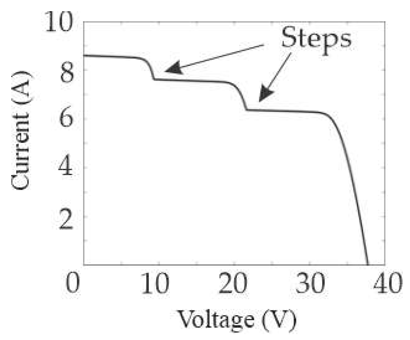
The presence of shading faults can be effectively diagnosed through analysis of the I–V curve, which exhibits characteristic changes in shape when such faults occur. In particular, as shown in Figure 2, non-uniform shading often results in the appearance of multiple steps or inflection points along the I–V curve [6,17,43], deviating from the smooth, single-knee profile seen in healthy modules. These distortions are caused by the activation of bypass diodes that limit reverse bias stress on shaded cells. As a result, the I–V curve may exhibit sudden drops in current or sharp changes in slope, signaling the existence and severity of partial shading. By analyzing these geometric changes, it is possible to not only detect the presence of shading but also to estimate its impact on the power output of the PV system.

2.4. Convolutinal Neural Networks

The diagnostic potential of I–V curves lies in their shape, which changes depending on the type and severity of faults, such as those caused by shading. Since these geometric deformations can be subtle or nonlinear, CNNs are well suited to this task, as they excel at recognizing patterns and local features in image-like data, making them ideal for the automatic analysis of I–V curves treated as visual patterns.
CNNs have significantly advanced deep learning by enabling high-accuracy image recognition and automatic feature extraction, reducing the need for manual engineering of features. This section provides an overview of CNN architecture and their mathematical foundations. CNNs are a class of deep neural networks specifically designed for spatially correlated data, such as images or structured matrices derived from time-series signals. A typical CNN consists of multiple stacked layers, including convolutional layers, pooling layers, and fully connected layers, which work together to extract hierarchical features from the input data [44]. The convolutional layer is the core component of a CNN, where feature extraction occurs. It applies a set of trainable filters (also called kernels) to the input data. Each filter slides across the input performing element-wise multiplications and summations, resulting in a feature map [45]. The number of filters (typically ranging from 4 to 128 or more per layer) and their kernel size (e.g., 3 × 3, 5 × 5, 8 × 8) are key architectural parameters that affect the network’s capacity to capture patterns at different scales. Mathematically, the convolution operation between an input image X and a filter W can be expressed as follows:
Y i , j = m n X i m , j n W m , n
where Y(i, j) is the output feature map at position (i, j) and W(m, n) represents the kernel weights. Following the convolution, pooling layers are applied to reduce the spatial dimensions of the feature maps, improving computational efficiency and enhancing translational invariance. The most common types are max pooling, which selects the highest value in a local window, and average pooling, which computes the mean value [46].
Toward the end of the architecture, fully connected layers aggregate the extracted features and map them to output predictions. The final classification is usually obtained through a softmax (for multi-class problems) or sigmoid (for binary classification) activation function [47].
CNN training involves optimizing the weights through backpropagation and gradient descent, guided by a loss function such as categorical cross-entropy or mean squared error [48]. The weight update rule is typically defined as follows:
W t + 1 = W t η L W
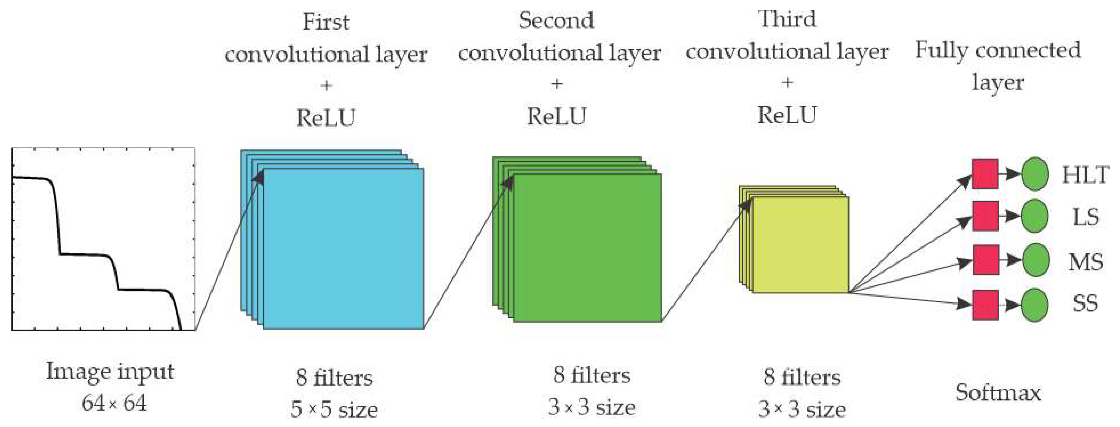
where η is the learning rate and L is the loss function. Common optimization algorithms include Stochastic Gradient Descent (SGD), Adam, and Root Mean Square Propagation RMSprop, which adaptively adjust learning rates to improve convergence speed and stability [49]. Figure 3 shows an example of a typical CNN.

3. Methodology

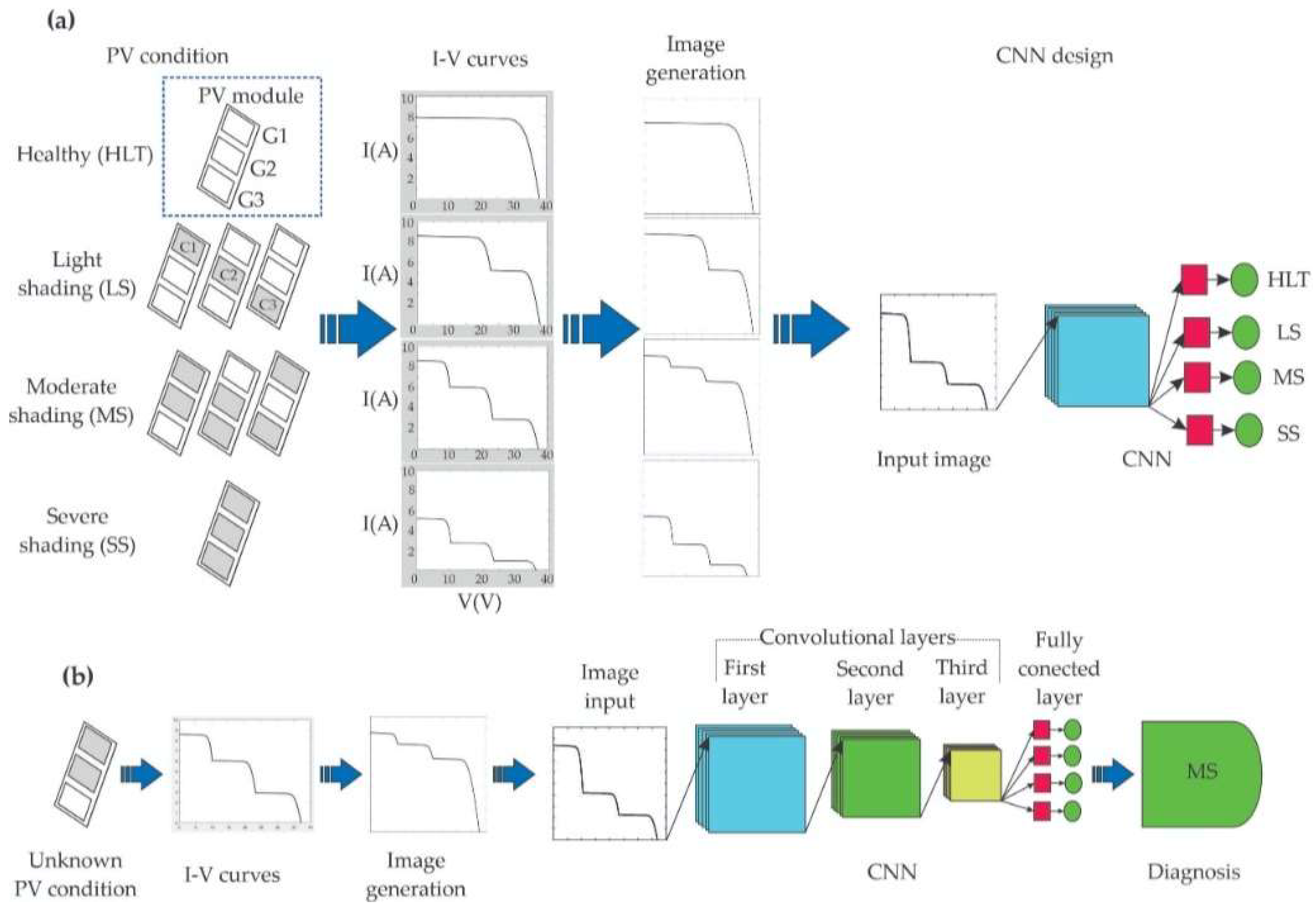
Figure 2 presents the proposed methodology for classifying shading conditions in PV modules using I–V curves and CNNs. As shown in Figure 4a, the system architecture includes a Simulink-based PV model composed of three groups of solar cells, labeled G1, G2, and G3 and highlighted within a blue rectangle. The objective is to classify into four different operating conditions: healthy (HLT), light shading (LS), moderate shading (MS), and severe shading (SS). These conditions are simulated by varying the irradiance levels applied to the cell groups. The HLT condition corresponds to all three groups receiving uniform irradiance, meaning that no significant environmental obstructions or dominant degradation effects are present. LS is defined when one of the three cell groups in the PV module (three possible cases: C1, C2, or C3) is subjected to reduced irradiance (represented by a gray block in Figure 4a). This situation may arise from environmental factors such as mild soiling or dust, thin cloud edges, or partial obstructions. MS occurs when two groups are shaded, mainly due to environmental issues, degradation, or localized shadows caused by string-level obstacles or dense soiling. Finally, SS refers to the case when all three groups are under shading, which may result from severe environmental and degradation effects, such as extensive cracks or hot-spots. It is important to note that for each shading scenario, the irradiance levels can differ between groups, resulting in distinct electrical behaviors and corresponding I–V curve shapes.
Each I–V curve generated under these scenarios is then converted into a grayscale image, forming the basis of the input dataset for CNN training and validation. Representative examples of these I–V curves are shown in Figure 5. To ensure a lightweight implementation, several custom-designed CNN architectures were evaluated by varying input resolution, filter sizes and counts, number of layers, and other hyperparameters. The goal was to find a balance between classification accuracy and model complexity. Once a suitable configuration was identified, the trained CNN was deployed following the procedure shown in Figure 4b: the I–V curve of an unknown PV module is acquired, transformed into an image, and analyzed by the CNN to determine the corresponding shading condition. The I–V image dataset was partitioned into 70% training, 15% validation, and 15% test, stratified by class (HLT/LS/MS/SS) and noise condition (noiseless, 10 dB); a fixed random seed was used. All augmentations were performed after the split to prevent leakage. Unless otherwise stated, performance is reported on the held-out test set. The next section details the technical specifications of the PV model, the simulation parameters, and the quantitative results.

4. Experimentation and Results

4.1. Experiment Setup

The experimental implementation models a standard 60-cell crystalline-silicon PV module wired as three series substrings, each substring comprising 20 cells in series, with one bypass diode connected antiparallel across each 20-cell substring. Thus, 60 series-connected cells form the module; under partial shading of any substring, its bypass diode activates and produces the characteristic step in the I–V curve observed in Figure 6, while the remaining substrings continue to deliver current. The authors intentionally adopted a series configuration at the module level because (i) it reflects how commercial modules are actually constructed (series substrings with bypass diodes), (ii) it meets typical inverter/MPPT voltage requirements while minimizing I2R losses, and (iii) it preserves the diagnostic signatures in the I–V curves (e.g., step regions due to bypass-diode activation) that the proposed CNN leverages. Note that the approach remains applicable regardless of the array interconnection used in the field (SP, BL, HC, or TCT).
Figure 6 presents the Simulink-based model of the PV module. Each group of 20 series-connected cells includes bypass diodes that enable current flow in the presence of shading or damage, ensuring continued power delivery. The module is connected to a variable DC voltage source to enable I–V curve acquisition under different irradiance conditions (Ir1, Ir2, and Ir3).
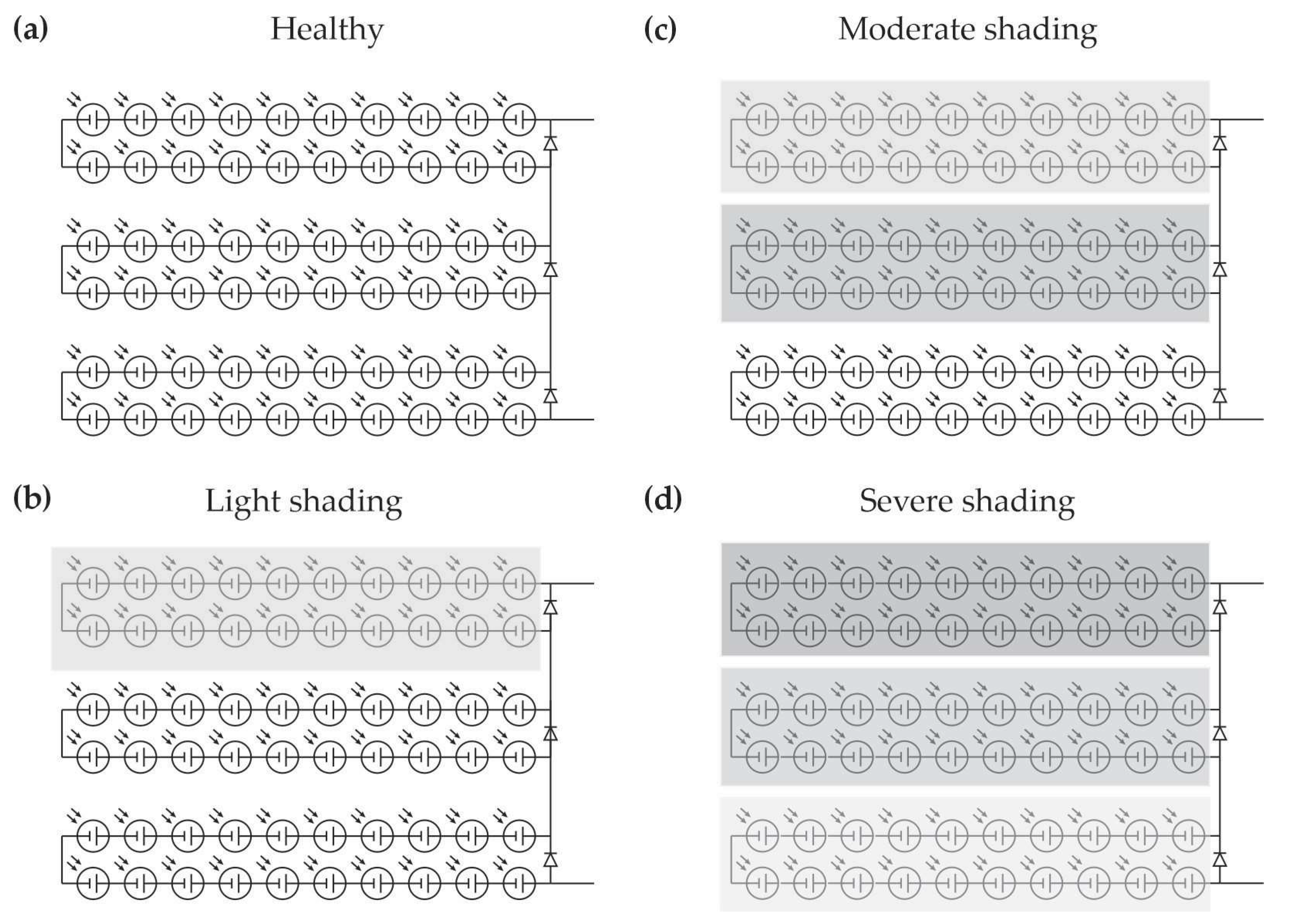
To evaluate the system’s response, four operating conditions are simulated by varying the irradiance applied to each of the three groups of cells. Figure 7 illustrates the specific shading patterns used in each scenario:
  • HLT: All three sections of 20 cells each receive uniform irradiance values (1000 W/m2 in Figure 4), representing the baseline performance of the module. Under uniform high irradiance, no bypass diode conducts. Consequently, the I–V curve exhibits a single knee with nominal Isc and Voc, and a high fill factor. The HLT label is assigned when all substrings remain forward-biased and no step features appear in the curve [11,40].
  • LS: A reduction in irradiance is applied to one section (either cells 1–20, 21–40, or 41–60), simulating partial obstruction such as mild dirt accumulation or small object shadows. Due to the non-uniform irradiance, the current produced by the shaded section cannot reach the total module current, causing its bypass diode to conduct. Therefore, the I–V curve exhibits a single shallow step corresponding to this partial bypass [10,11].
  • MS: Two of the three sections are subjected to reduced irradiance. For example, string 2 (cells 21–40) receives 300 W/m2, while string 3 (cells 41–60) receives 600 W/m2. This configuration simulates more significant power loss and uneven shadowing. In this case, the shaded substrings are reverse-biased when the total current exceeds their maximum output, activating their bypass diodes and producing two steps in the I–V curve [11,40].
  • SS: All three sections are shaded, each with different irradiance levels to reflect highly variable conditions. This setup represents the most critical degradation scenario for power output and voltage stability. Substrings are bypassed as their diodes conduct when their current limits are exceeded, and the I–V curve shows two steps along with a substantial reduction in voltage and power [40,41].
These varying irradiance levels, shading scenarios, and even extreme variations in the I–V curves are intentionally induced in the Simulink model of Figure 6 to generate a wide range of curve shapes (different classes). These curves are subsequently used for training and validating the CNN, as the main goal of this work is to test its performance in differentiating among the classes. The complete dataset includes 1000 I–V curves for each class, with irradiance values randomly selected, considering 1000 W/m2 as the maximum irradiance level. All simulations, data preprocessing, and CNN training/validation were executed exclusively on CPU (laptop with 2.30 GHz CPU, 16 GB RAM, 64-bit OS) in MATLAB R2024a (Deep Learning Toolbox); no GPU acceleration was used.

4.2. CNN Results

One of the central goals of this study was to investigate whether custom-designed CNNs, when carefully configured through systematic experimentation, could achieve high classification performance for partial shading conditions in PV modules, without relying on complex architectures or optimization algorithms. Instead of employing techniques like Bayesian search or genetic algorithms, this work demonstrates that iterative, structured testing of basic architectural parameters can be sufficient to achieve excellent results, while preserving simplicity and interpretability.
The decision to use custom CNNs is justified by the fact that shading-induced changes in I–V curves are relatively subtle and highly structured. This allows CNNs, even with shallow depths, to capture meaningful features without the need for transfer learning or pre-trained models. Moreover, this strategy simplifies deployment in low-power embedded systems, aligning with the ultimate objective of building lightweight, real-time diagnostic tools.
The model development followed a progressive refinement strategy. The process began with a single convolutional layer to explore the effects of varying the number of filters and their size. Then, additional convolutional layers were added one by one, optimizing the architecture incrementally. Finally, the image resolution was reduced to analyze the impact on classification performance and computational efficiency. This staged approach ensured transparency in the architectural design and facilitated interpretation of performance gains.

4.2.1. Evaluation of the Convolutional Layers

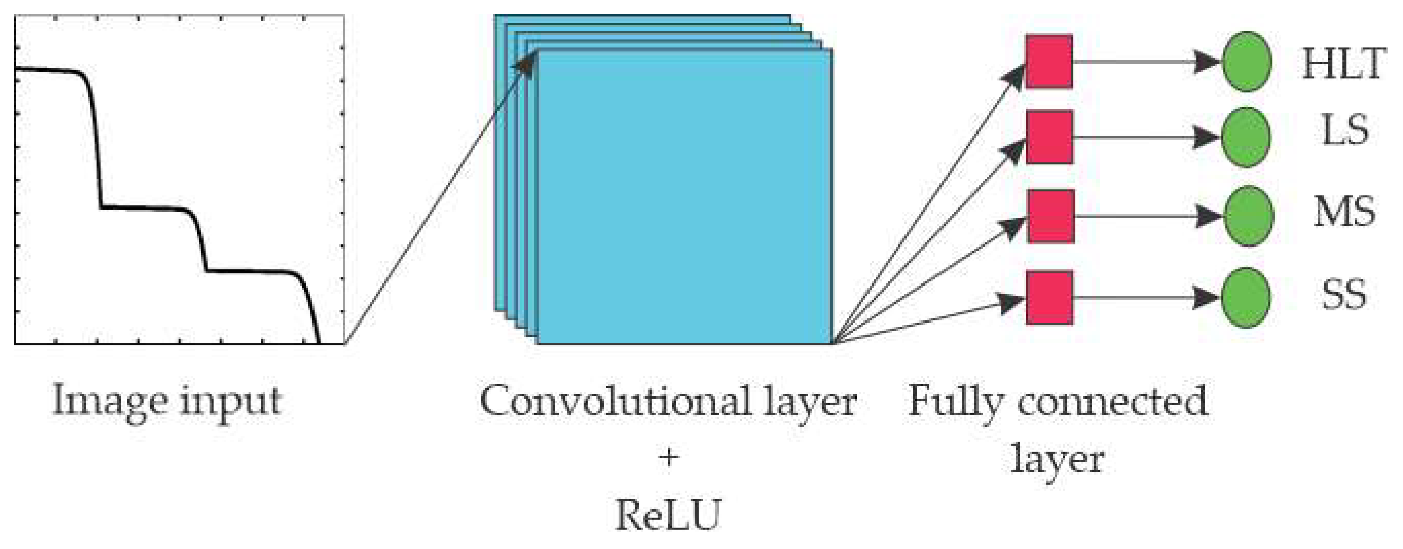
The initial stage of the CNN design involved testing single-layer architectures to evaluate their ability to discriminate between the four shading conditions: healthy, light, moderate, and severe. Each convolutional layer uses the ReLU (Rectified Linear Unit) activation function to introduce non-linearity, followed by max-pooling operations to reduce spatial dimensions while preserving the most salient features [50]. At the output layer, the network consists of four neurons, each corresponding to one of the shading categories (see Figure 8). These output neurons are activated according to the predicted condition of the PV module, which is carried out through a SoftMax activation function, which converts the output logits into probability scores for each class. The model was trained using the Adam optimizer with a learning rate of 0.001, ensuring efficient and stable convergence during training [50].
To assess the performance of the first convolutional layer, two key hyperparameters are systematically varied:
  • Number of filters: 4, 8, 16, and 32
  • Filter sizes: 3 × 3, 5 × 5, and 8 × 8
As shown in Table 1, the configuration using eight filters of size 5 × 5 achieved the highest classification accuracy, reaching 95.8% (indicated by a green rectangle). While the 8 × 8 filter was also evaluated and showed comparable performance, the 5 × 5 filters yielded slightly better results, possibly due to a better spatial feature capture; additionally, smaller filters were preferred to reduce complexity. It is worth noting that the results shown in Table 1 are average values obtained over five runs, with a maximum standard deviation of 0.16%, indicating high consistency and robustness of the model’s performance. Furthermore, the low standard deviation indicates that the classification results are stable across runs and that there is minimal or null overlap between configurations, reinforcing the reliability of the selected architecture.
These specific values were selected to explore a range of complexity levels: a small number of filters allows for fast execution and low computational cost, while larger filter sizes capture more global features in the I–V curve images. This systematic exploration demonstrates that even without optimization algorithms, an efficient architecture can be derived through guided testing of reasonable configurations.
After selecting the best configuration for a single-layer CNN, the architecture was extended by progressively adding convolutional layers to evaluate the impact of network depth on classification performance. In this phase, configurations with two, three, and four convolutional layers were systematically explored.
To design the two-layer architecture, the selected configuration from the first layer (eight filters of 5 × 5) was maintained, while the second layer was varied in terms of number and size of filters. Table 2 presents the performance of these configurations, with the best result obtained using eight filters of size 3 × 3, achieving an accuracy of 96.9%. This result highlighted that adding a second layer allowed the network to capture more abstract features while maintaining relatively low computational complexity.
Subsequently, a third convolutional layer was introduced. The first and second layers were fixed using the selected settings from the previous stage (eight filters of 5 × 5 and eight filters of 3 × 3, respectively), and the third layer was varied. As shown in Table 3, the best configuration used eight filters of 3 × 3 in the third layer, increasing classification accuracy to 99.5%. These results demonstrate that a deeper network can significantly enhance performance by enabling hierarchical feature extraction.
Finally, a fourth convolutional layer was evaluated to assess whether further depth could improve classification. The first three layers used the previously selected parameters, while the fourth layer was tested with several combinations of filter numbers and sizes, similarly to earlier stages. However, the addition of a fourth layer did not improve performance and led to increased training complexity. This can be attributed to the relatively low complexity of the classification task and the limited resolution of the input images, which do not require very deep architectures to achieve high performance.
It is worth noting that throughout all experiments with two to four layers, the number of filters remained at eight for the first three layers, indicating that this number provided a good balance between model capacity and feature extraction. Regarding filter sizes, the optimal configuration consistently used a larger filter (5 × 5) in the first layer, followed by smaller filters (3 × 3) in subsequent layers. This design allows the network to first extract coarse-grained spatial features and then progressively refine these representations at finer scales, which is a common and effective strategy in CNN design. Figure 9 shows the final CNN architecture.

4.2.2. Evaluation of Image Resolution

After improving the CNN architecture using 512 × 512 input images, an additional evaluation was conducted to analyze the impact of reducing image resolution on classification accuracy. The goal was to minimize computational cost without significantly affecting performance. The following resolutions were tested: 256 × 256, 128 × 128, 64 × 64, and 32 × 32. Figure 10 illustrates examples of I–V curve images at these different resolutions, included for demonstrative purposes to visually highlight the progressive reduction in spatial detail.
It is important to note that when the input image size is modified, the previously selected architecture, specifically, the number of layers, filters, and filter sizes, could require adjustments, as these parameters are often influenced by the scale and level of detail in the input data. Nevertheless, in this study, the same CNN configuration was retained to ensure a fair comparison across different resolutions and to isolate the impact of input size alone. In this regard, the model demonstrated high robustness, maintaining accuracy above 99% even at 64 × 64 resolution, and only a moderate drop at 32 × 32 (see Table 4).
These findings suggest that the architecture, although initially tuned for high-resolution inputs, generalizes well across different resolutions. This can be attributed to the relatively simple nature of the classification task, detecting four well-defined shading patterns, as well as the effectiveness of the feature extraction layers in capturing the essential characteristics of the I–V curves despite reduced spatial detail.
The configuration using 64 × 64 images was selected as the final input resolution, as it offers a suitable trade-off between accuracy and computational efficiency, making it suitable for implementation in real-time embedded systems with limited resources.

4.2.3. Final Configuration and Training Performance

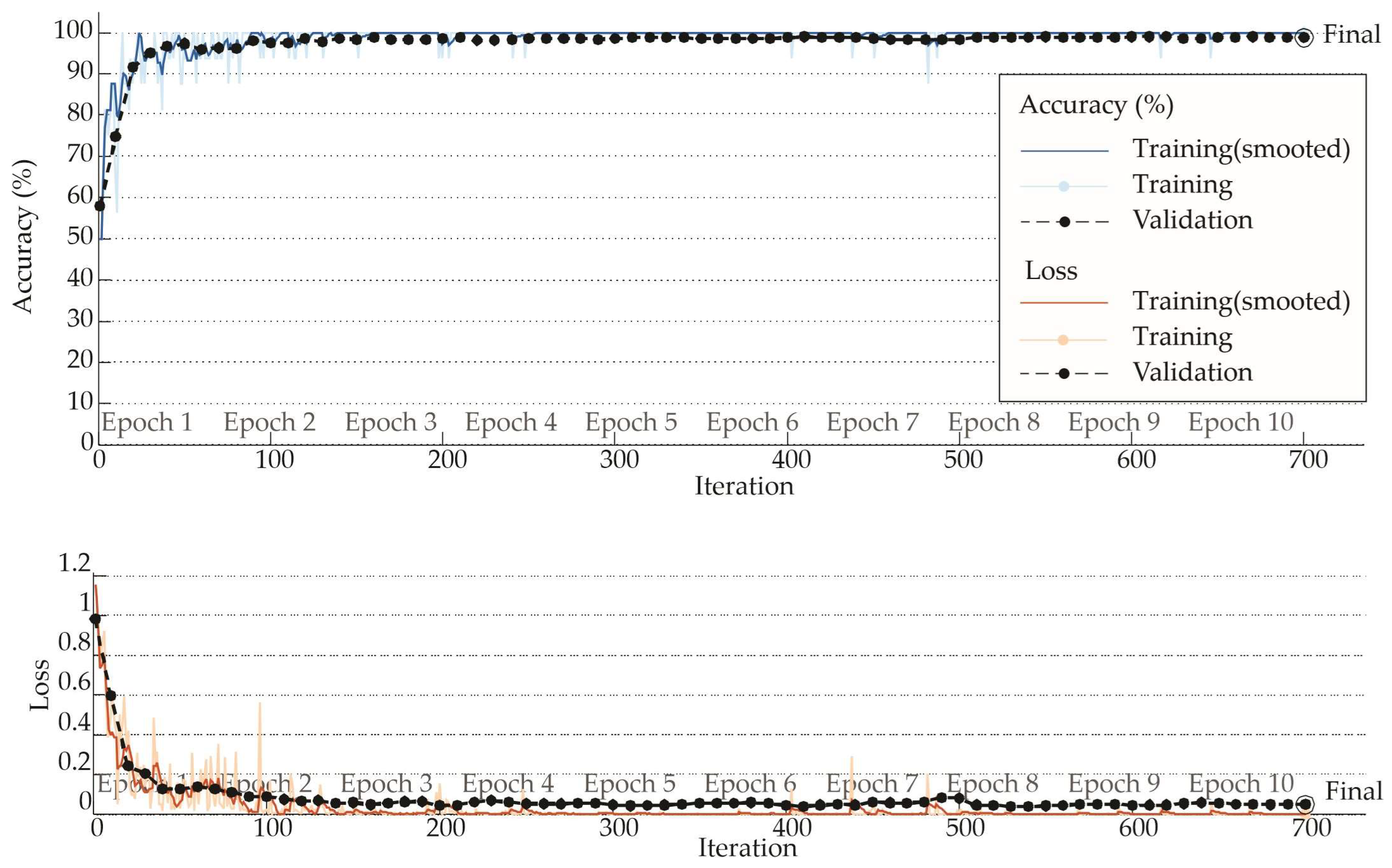
Figure 11 presents the training and validation accuracy and loss curves for the selected configuration. This final model consists of the following:
  • Input resolution: 64 × 64 pixels.
  • CNN structure: three convolutional layers with eight filters (first layer: 5 × 5, second: 3 × 3, third: 5 × 5).
  • Stride and padding: stride = 1, same padding for all layers.
  • Pooling: two max-pooling layers with pool size 2 × 2.
  • Activation functions: ReLU for convolutional layers and softmax for classification.
  • Cross-validation: k-fold used, with k = 5, to ensure robustness of results.
  • Training parameters: batch size = 32, epochs = 10, optimizer = Adam, learning rate = 0.001, early stopping not applied due to convergence in under 10 epochs.
  • Conventional dataset split: 70% training, 15% validation, 15% testing.
Table 5 shows the remaining CNN settings.
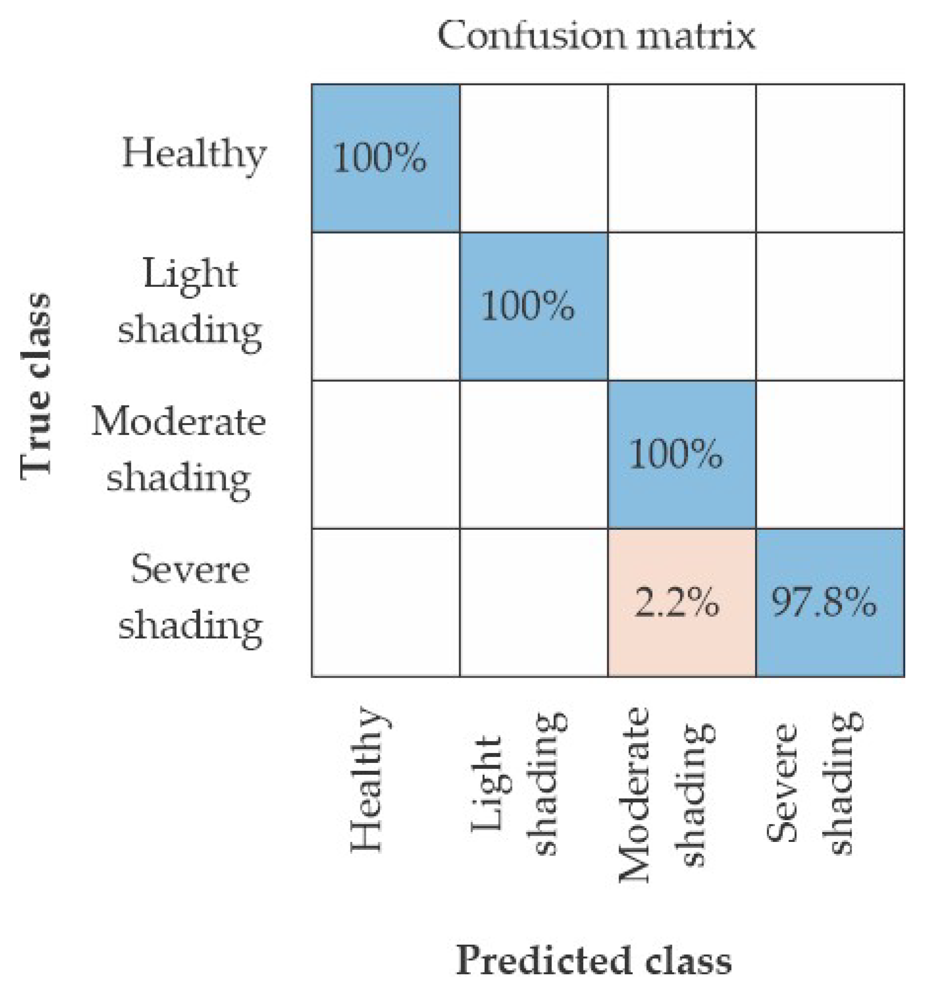
The confusion matrix in Figure 12 confirms the effectiveness of the classification, with nearly all test samples correctly identified, obtaining an average accuracy of 99.5%. As can be observed, classification errors occurred only in the moderate shading condition; that is, some severe shading cases were misclassified as moderate shading. However, this is not critical, as it still indicates a faulty condition and remains closer to the severe category. These results support the conclusion that custom CNN architectures, when properly tuned through systematic experimentation, offer a competitive and efficient solution for real-time diagnostics in solar PV systems.
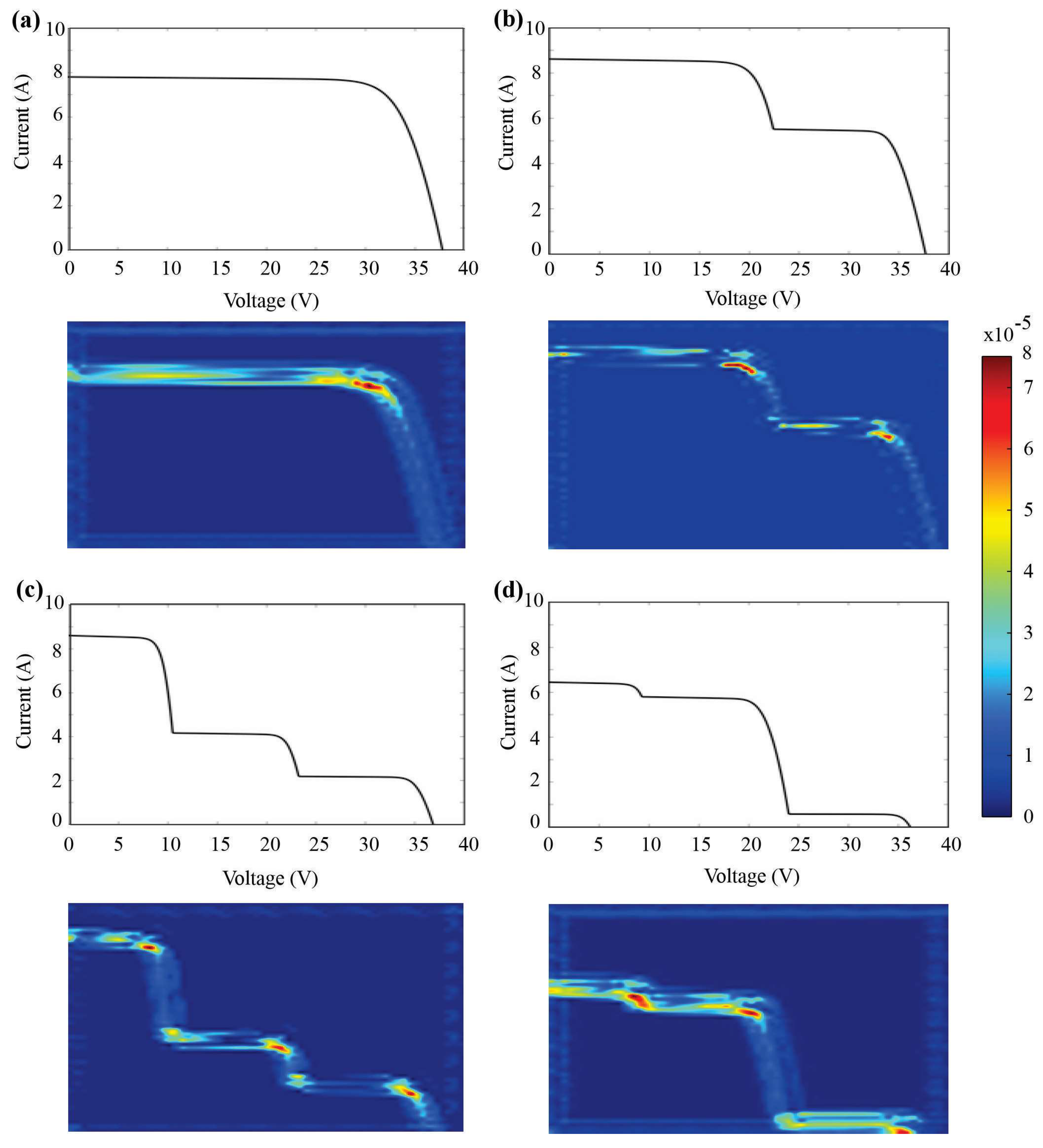
The final CNN is deliberately compact (≈104 parameters), which limits memorization. The training and validation curves in Figure 11 overlap closely with no late-epoch divergence, indicating a small generalization gap during optimization. Additionally, 5-fold (k = 5) cross-validation confirmed stable performance across folds. Performance is reported on a held-out test split (15%) unseen during training/validation, achieving 99.5% under noiseless conditions and 90.1% at 10 dB SNR (Section 4.4), which evidences robustness to distributional perturbations. Moreover, Gradient-Weighted Class Activation Mapping (Grad-CAM), as will be discussed in the next subsection, highlights that the model focuses on physically meaningful I–V inflection regions (e.g., step zones from bypass-diode activation), reinforcing that the classifier leverages diagnostic structure rather than spurious artifacts.
In addition to the confusion matrix analysis, global performance metrics were calculated to provide a more comprehensive evaluation of the model. The proposed CNN achieved an overall accuracy of 98.96%, with macro-precision, macro-recall, and macro-F1 scores of 98.08%, 97.92%, and 97.91%, respectively. When weighted by class support, the precision, recall, and F1-score reached 99.04%, 98.96%, and 98.96%, respectively. These results confirm that the proposed architecture maintains balanced and robust performance across all shading severity conditions, further reinforcing its suitability for real-time PV fault diagnosis.

4.3. Gradient-Weighted Class Activation Mapping (Grad-CAM) Results

To enhance the interpretability of the proposed CNN model and better understand how it distinguishes between healthy and shaded PV module conditions, Grad-CAM is applied [51]. Grad-CAM is a visualization technique that produces class-discriminative heatmaps highlighting the regions of the input that most influence the network’s decisions. In the context of this study, Grad-CAM helps reveal which segments of the I–V curve images contribute the most to the classification of each condition. Understanding which regions of the I–V curve drive the CNN’s classification can be crucial for building trust in automated diagnostic systems, particularly in safety-critical or high-reliability applications such as solar energy monitoring. Additionally, explainability methods like Grad-CAM can help verify that the model is learning relevant features rather than relying on spurious correlations.
Figure 13 presents the Grad-CAM visualizations for four representative I–V curves: (a) healthy, (b) light shading, (c) moderate shading, and (d) severe shading. According to the color intensity bar, the most activated regions, those contributing most to the classification, are located in portions of the curve where slope changes occur. These inflection points are directly related to the electrical distortions caused by shading. In contrast, regions of the curve where the slope is constant or nearly linear exhibit minimal contribution to the classification process. This behavior confirms that the CNN has learned to focus on physically meaningful features associated with fault conditions.

4.4. Robustness Evaluation Under Noisy Conditions

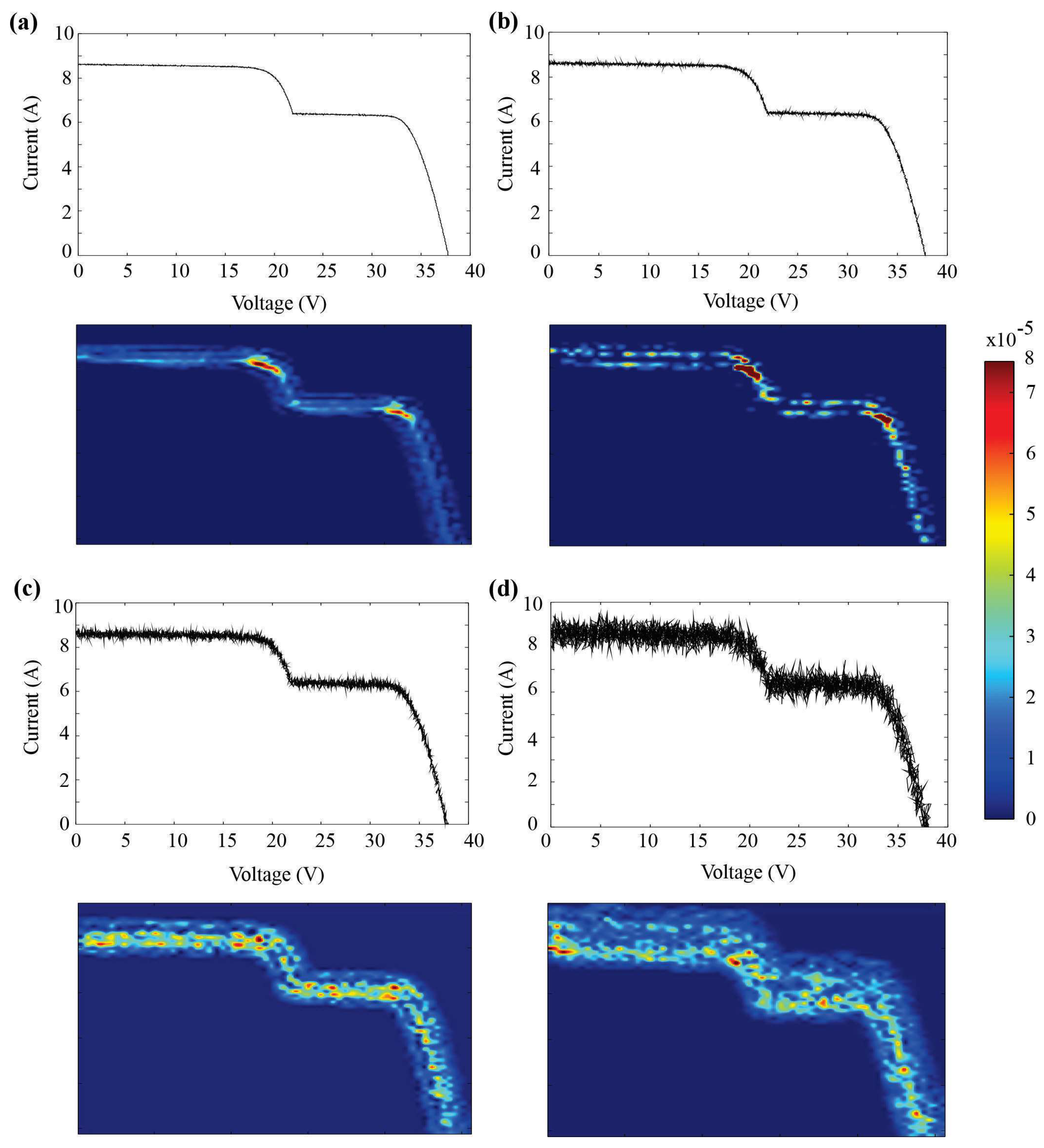
To assess the robustness and noise immunity of the proposed CNN-based classification model, an additional set of experiments was conducted using I–V curves contaminated with different levels of noise in real-world scenarios; measurement noise can be introduced by environmental factors, sensor imperfections, or electronic interference in data acquisition systems. In photovoltaic systems, such noise may arise from temperature fluctuations, panel soiling, inverter switching transients, or electromagnetic interference from nearby electrical equipment [11]. To simulate these conditions, white Gaussian noise was added to the test signals at four different signal-to-noise ratio (SNR) levels: 40 dB, 30 dB, 20 dB, and 10 dB. Among these, 10 dB represents the most severe case, which is intentionally exaggerated and may not be realistic but serves to evaluate the model’s limits.
Figure 14 illustrates examples of I–V curves affected by each noise level: (a) 40 dB, (b) 30 dB, (c) 20 dB, and (d) 10 dB. It can be observed that as the noise level increases (i.e., SNR decreases), the curve distortion becomes more evident, potentially affecting the model’s decision-making. In the same figure, the Grad-CAM visualizations are included to reveal how the CNN makes its predictions. These activation maps show that regions corresponding to inflection points or slope changes in the I–V curves, caused by shading, contribute most to the decision process. Even at higher noise levels, although the prominence of these key areas diminishes, they still contribute meaningfully, demonstrating the model’s ability to maintain classification performance despite increasing noise.
Additionally, Figure 15 presents the classification accuracy results across different noise levels. For this evaluation, 15% of the I–V curves used during testing (as described in Section 3) were contaminated with the aforementioned noise levels. The resulting classification accuracies were 99.4%, 97.2%, 94.4%, and 90.1% for 40 dB, 30 dB, 20 dB, and 10 dB, respectively. Notably, the performance at 40 dB was nearly identical to the noise-free case, indicating that mild noise does not significantly affect the CNN’s reliability. Even under the most severe noise condition (10 dB), the model maintained an accuracy of 90.1%, demonstrating its high robustness and ability to generalize despite substantial signal degradation.

5. Discussion

This study demonstrates that custom-designed CNNs offer a viable and effective solution for classifying different shading conditions in PV modules using I–V curves as input. These curves are typically obtained using specialized measurement devices such as I–V curve tracers, implying that the proposed CNN-based diagnostic approach could be directly integrated into such systems to automate fault detection and classification. This automation can reduce the likelihood of human error in visual inspection or manual interpretation, streamline field diagnostics, and enable early detection of performance issues in PV installations [2,11].
A modular Simulink-based simulation platform was used to emulate a segmented PV module composed of three parallel strings. This design allowed for precise and systematic manipulation of irradiance across the module, enabling the simulation of four representative shading conditions: HLT, LS, MS, and SS. By varying irradiance levels, the model accurately mimicked real-world effects such as soiling, partial obstruction from nearby objects, or cloud shadows. Unlike physical experimental setups, the use of a simulation model offers controlled and repeatable testing scenarios [43], eliminates environmental noise, and enables exhaustive exploration of edge cases that would be impractical or costly to replicate in physical hardware.
A series of progressively refined CNN architectures were developed and tested. The initial single-layer CNN with eight filters of size 5 × 5 yielded an average accuracy of 95.8%, showing the feasibility of using compact models for this classification task. A two-layer CNN, building on the optimal first-layer configuration, improved performance to 96.8% (average). Adding a third convolutional layer further boosted average accuracy to 99.5%, confirming that deeper networks can capture more abstract and complex features in I–V curve images. Importantly, these improvements were achieved while maintaining a low computational load, with the final architecture remaining lightweight and efficient compared to traditional, pre-trained models such as AlexNet [32]. A key finding of this study is that high classification accuracy can be retained even with significantly reduced input image resolution. Reducing image size from 512 × 512 to 64 × 64 pixels led to the highest accuracy of 99.5% (average), suggesting that essential features for classification, such as slope changes in I–V curves, are preserved even at lower resolutions. This result highlights the suitability of the proposed method for embedded applications and real-time diagnostic systems, where processing speed and memory efficiency are crucial.
To assess the model’s robustness to measurement noise, Gaussian noise with varying intensity was added to the I–V curves. The results showed that the CNN maintained high classification performance under noisy conditions, i.e., 90.1% (average), with only minor degradations observed at the highest noise levels (10 dB). This robustness reinforces the practicality of the approach for deployment in real environments, where electrical measurements are often affected by sensor noise, electromagnetic interference, and fluctuations in operating conditions [11]. Explainability was addressed using gradient-weighted class activation mapping (Grad-CAM). The heatmaps revealed that the CNN focuses primarily on the inflection zones of the I–V curve, regions where slope changes occur due to shading-induced anomalies. These results confirm that the CNN is learning meaningful features, rather than overfitting to irrelevant artifacts. This automatic feature extraction parallels the use of handcrafted indicators in traditional diagnostic techniques and represents a key advantage of deep learning approaches. It is worth noting that to adapt the proposed CNN to multi-fault classification, modifications to the output layer would be required to accommodate additional fault classes. Importantly, Grad-CAM analysis has shown that the network primarily focuses on slope changes in the I–V curves, which are key features affected by various types of PV faults. This indicates that the architecture can generalize effectively to other fault types, providing interpretable visualizations that could support human-in-the-loop diagnosis in real-time monitoring scenarios.
Although CNNs are a well-established deep learning technique, their simplicity, robustness, and proven ability to extract spatial features make them highly suitable for the analysis of I–V curve images. The novelty of this work does not lie in proposing a new algorithm but in demonstrating that lightweight, custom-designed CNNs can achieve state-of-the-art accuracy while remaining computationally efficient and practical for embedded PV diagnostic applications. Unlike other approaches that rely on complex, pre-trained models requiring transfer learning and extensive computational resources, the proposed lightweight architecture achieves comparable or even superior performance at a significantly lower computational cost. This efficiency makes it particularly suitable for integration into portable I–V tracers or low-power microcontrollers, thereby enabling on-site, real-time health monitoring in remote solar installations and in low-cost diagnostic systems.
In general, compact CNN architectures such as MobileNet-V2 and ShuffleNet-V2 are widely recognized as lightweight; however, they were originally designed for large-scale RGB image classification (ImageNet) and still involve millions of parameters and high computational cost [52,53,54]. In contrast, the proposed custom-designed CNNs are specifically tailored for grayscale I–V curve images, requiring two orders of magnitude fewer parameters while preserving accuracy, which makes them suitable for real-time deployment in embedded PV diagnostic systems. Similarly, classical approaches based on machine learning are not directly comparable, since they rely on handcrafted feature extraction rather than end-to-end learning from images.
Despite these promising results, this study has some limitations. The approach has been validated on simulated I–V data, which, while realistic and informative, does not capture all the complexities of real-world PV systems, such as temperature variations, aging effects, inverter behavior, sensor drift, or other hardware-induced nonidealities. These aspects were not considered in this work, as the primary objective was to design and evaluate a custom CNN specifically tailored for detecting and classifying shading faults. Future work will focus on validating the model with field data, expanding the scope to include additional fault types (e.g., hotspot formation, degradation), and exploring optimization algorithms, such as genetic algorithms or particle swarm optimization, to automatically tune the CNN architecture. Moreover, hardware implementation on low-cost embedded systems will be explored to transition from simulation to practical deployment in intelligent PV monitoring platforms. This staged approach ensures that the current study provides a proof-of-concept for the effectiveness of lightweight, task-specific CNNs, while acknowledging the need for further validation under more diverse real-world conditions.

6. Conclusions

This work investigates the potential of custom-designed CNNs for the automated classification of shading conditions in PV modules using I–V curves as input data. These curves, typically acquired through I–V tracers or integrated monitoring systems, provide a compact yet informative representation of the module’s electrical behavior. By exploring CNNs specifically tailored for this task, rather than relying on complex pre-trained architectures, this study contributes to an emerging area of research with limited prior exploration. The results demonstrate that even simple CNN architectures can effectively learn and differentiate subtle variations in curve morphology induced by partial shading.
A key strength of the proposed approach lies in its robustness and reduced computational structure. The CNN maintained high classification accuracy under varying image resolutions and different levels of additive noise (up to 10 dB), achieving a maximum accuracy of 99.5% with input images of only 64 × 64 pixels. This highlights the feasibility of applying the method in real-time and embedded applications where memory and processing power are constrained. Furthermore, Grad-CAM visualizations revealed that the network focuses on physically relevant inflection zones in the I–V curves, confirming that the CNN extracts meaningful features rather than learning spurious correlations.
The development of a modular Simulink-based simulation platform allowed for the systematic and repeatable emulation of different shading scenarios, i.e., healthy, light, moderate, and severe, ensuring a controlled evaluation framework. While the findings are encouraging, the current study is based solely on simulated data. Future research will focus on validating the approach using field-acquired I–V measurements, extending the method to detect additional fault types, and exploring optimization techniques for automatic CNN tuning. Ultimately, the integration of lightweight CNNs into portable I–V tracers or embedded devices could enable low-cost, real-time diagnostic systems, supporting the advancement of intelligent and autonomous solar energy technologies. Future research will focus on validating the approach using field-acquired I–V measurements, extending the method to detect additional fault types such as hotspots, cracked cells, and bypass diode failures, and exploring optimization techniques such as genetic algorithms, particle swarm optimization, or Bayesian optimization for automatic CNN architecture tuning. An experimental test bench is being developed to induce controlled shading levels and obtain realistic I–V curves, followed by data collection under real operating conditions. This staged process will enable stronger validation and facilitate practical deployment in PV monitoring scenarios.

Author Contributions

Conceptualization, J.A.A.-P., A.H.R.-R. and M.V.-R.; methodology, J.A.A.-P., A.H.R.-R. and M.V.-R.; software, formal analysis, resources, and data curation, J.A.A.-P. and A.H.R.-R.; writing—review and editing, all authors; supervision, project administration, and funding acquisition, J.P.A.-S., D.G.-L., G.T.-T. and M.V.-R. All authors have read and agreed to the published version of the manuscript.

Funding

This research was supported by the “Modelado y análisis de fallas en celdas solares por sombreado parcial” project funded under the “Convocatoria 2025: Proyectos de Investigación Científica, Desarrollo Tecnológico e Innovación”.

Data Availability Statement

The original contributions presented in this study are included in the article. Further inquiries can be directed to the corresponding author.

Acknowledgments

Thanks to the “Secretaría de Ciencia, Humanidades, Tecnología e Innovación (SECIHTI)—México” that partially financed this research under the scholarships 169320 and 830903 given to Jesus A. Arenas-Prado and Angel H. Rangel-Rodriguez, respectively, and the support given to David Granados-Lieberman, Guillermo Tapia-Tinoco, Juan P. Amezqui-ta-Sanchez, and Martin Valtierra-Rodriguez through the “Sistema Nacional de Investigadoras e Investigadores (SNII)–SECIHTI–México”.

Conflicts of Interest

The authors declare no conflict of interest.

Abbreviations

The following abbreviations are used in this manuscript:
PVPhotovoltaic
CNNConvolutional neural network
ANNArtificial neural network
DCDirect current
HLTHealthy
LSLight shading
MSModerate shading
ReLUSevere shading
Grad-CAMGradient-weighted class activation mapping
SNRSignal-to-noise ratio

References

  1. Sayed, E.T.; Olabi, A.G.; Alami, A.H.; Radwan, A.; Mdallal, A.; Rezk, A.; Abdelkareem, M.A. Renewable energy and energy storage systems. Energies 2023, 16, 1415. [Google Scholar] [CrossRef]
  2. Obeidat, F. A comprehensive review of future photovoltaic systems. Sol. Energy 2018, 163, 545–551. [Google Scholar] [CrossRef]
  3. Uddin, M.; Kazemi, A. A Fault Detection Scheme Utilizing Convolutional Neural Network for PV Solar Panels with High Accuracy. In Proceedings of the 2022 IEEE 1st Industrial Electronics Society Annual On-Line Conference (ONCON), Indian Institute of Technology Kharagpur, Virtual Conference, Kharagpur, India, 9–11 December 2022; pp. 1–5. [Google Scholar] [CrossRef]
  4. Khan, M.; Khan, A.; Ahmad, Z.; Khan, S.; Mohammed, A. A Model-Based Approach for Detecting and Identifying Faults on the D.C. Side of a P.V. System Using Electrical Signatures from I-V Characteristics. PLoS ONE 2022, 17, e0260771. [Google Scholar] [CrossRef]
  5. Lin, W.-T.; Chang, C.-M.; Huang, Y.-C.; Wu, C.-C.; Kuo, C.-C. Fault Diagnosis in Solar Array I-V Curves Using Characteristic Simulation and Multi-Input Models. Appl. Sci. 2024, 14, 5417. [Google Scholar] [CrossRef]
  6. Khan, Z.U.; Khan, A.D.; Khan, K.; Al Khatib, S.A.K.; Khan, S.; Khan, M.Q.; Ullah, A. A Review of Degradation and Reliability Analysis of a Solar PV Module. IEEE Access 2024, 12, 185036–185054. [Google Scholar] [CrossRef]
  7. Mustafa, R.J.; Gomaa, M.R.; Al-Dhaifallah, M.; Rezk, H. Environmental Impacts on the Performance of Solar Photovoltaic Systems. Sustainability 2020, 12, 608. [Google Scholar] [CrossRef]
  8. Köntges, M.; Kurtz, S.; Packard, C.; Jahn, U.; Berger, K.A.; Kato, K.; Friesen, T.; Liu, H.; Van Iseghem, M. Review of Failures of Photovoltaic Modules; Report IEA-PVPS T13-01:2014; International Energy Agency Photovoltaic Power Systems Programme: Paris, France, 2014. [Google Scholar]
  9. Virtuani, A.; Pavanello, D.; Friesen, T.; Caccivio, M.; Leanza, G.; Ballif, C. The Ageing of Crystalline Silicon Photovoltaic Modules: Materials and Performance. Renew. Energy 2021, 163, 1891–1907. [Google Scholar]
  10. Meyer, E.L.; van Dyk, E.E. Assessing the Reliability and Degradation of Photovoltaic Module Performance Parameters. IEEE Trans. Reliab. 2004, 53, 83–92. [Google Scholar] [CrossRef]
  11. Luque, A.; Hegedus, S. (Eds.) Handbook of Photovoltaic Science and Engineering; Wiley: Chichester, UK, 2003. [Google Scholar]
  12. Villalva, M.G.; Gazoli, J.R.; Filho, E.R. Comprehensive Approach to Modeling and Simulation of Photovoltaic Arrays. IEEE Trans. Power Electron. 2009, 24, 1198–1208. [Google Scholar] [CrossRef]
  13. Vieira, R.G.; de Araújo, F.M.U.; Dhimish, M.; Guerra, M.I.S. A Comprehensive Review on Bypass Diode Application on Photovoltaic Modules. Energies 2020, 13, 2472. [Google Scholar] [CrossRef]
  14. Özkalay, E.; Valoti, F.; Caccivio, M.; Virtuani, A.; Friesen, G.; Ballif, C. The Effect of Partial Shading on the Reliability of Photovoltaic Modules in the Built-Environment. EPJ Photovolt. 2024, 15, 7. [Google Scholar] [CrossRef]
  15. Zbib, B.; Al-Sheikh, H. Fault Detection and Diagnosis of Photovoltaic Systems through I-V Curve Analysis. In Proceedings of the 2020 International Conference on Electrical, Communication, and Computer Engineering (ICECCE), Istanbul, Turkey, 12–13 June 2020; pp. 1–6. [Google Scholar] [CrossRef]
  16. Fadhel, S.; Migan, A.; Delpha, C.; Diallo, D.; Bahri, I.; Trabelsi, M.; Mimouni, M. Data-Driven Approach for Isolated PV Shading Fault Diagnosis Based on Experimental I-V Curves Analysis. In Proceedings of the 2018 IEEE International Conference on Industrial Technology (ICIT), Lyon, France, 20–22 February 2018; pp. 927–932. [Google Scholar] [CrossRef]
  17. Hopwood, M.; Stein, J.; Braid, J.; Seigneur, H. Physics-Based Method for Generating Fully Synthetic IV Curve Training Datasets for Machine Learning Classification of PV Failures. Energies 2022, 15, 5085. [Google Scholar] [CrossRef]
  18. Lu, S.; Wang, M.-H.; Wei, S.-E.; Liu, H.D.; Wu, C.-C. Photovoltaic Module Fault Detection Based on a Convolutional Neural Network. Processes 2021, 9, 1635. [Google Scholar] [CrossRef]
  19. Fadhel, S.; Delpha, C.; Diallo, D.; Bahri, I.; Migan, A.; Trabelsi, M.; Mimouni, M. PV Shading Fault Detection and Classification Based on I-V Curve Using Principal Component Analysis: Application to Isolated PV System. Sol. Energy 2018, 179, 1–10. [Google Scholar] [CrossRef]
  20. Pierdicca, R.; Malinverni, E.; Piccinini, F.; Paolanti, M.; Felicetti, A. Deep Convolutional Neural Network for Automatic Detection of Damaged Photovoltaic Cells. In Proceedings of the ISPRS—International Archives of the Photogrammetry, Remote Sensing and Spatial Information Sciences, Göttingen, Germany, 10–12 May 2018; Volume XLII-2, pp. 893–900. [Google Scholar] [CrossRef]
  21. Spataru, S.; Sera, D.; Kerekes, T.; Teodorescu, R. Diagnostic method for photovoltaic systems based on light I–V measurements. Sol. Energy 2015, 119, 29–44. [Google Scholar] [CrossRef]
  22. Bressan, M.; El Basri, Y.; Gutierrez, A.; Alonso, C. A Shadow Fault Detection Method Based on the Standard Error Analysis of I-V Curves. Renew. Energy 2016, 99, 1181–1190. [Google Scholar] [CrossRef]
  23. Zabihi, A.; Sadeghkhani, I.; Fani, B. A partial shading detection algorithm for photovoltaic generation systems. J. Sol. Energy Res. 2021, 6, 678–687. [Google Scholar]
  24. Yuan, Z.; Xiong, G.; Fu, X. Artificial Neural Network for Fault Diagnosis of Solar Photovoltaic Systems: A Survey. Energies 2022, 15, 8693. [Google Scholar] [CrossRef]
  25. Hopwood, M.; Gunda, T.; Seigneur, H.; Walters, J. Neural Network-Based Classification of String-Level IV Curves from Physically-Induced Failures of Photovoltaic Modules. IEEE Access 2020, 8, 161480–161487. [Google Scholar] [CrossRef]
  26. Nehme, B.; M’Sirdi, N.; Namaane, A.; Akiki, T. Analysis and Characterization of Faults in PV Panels. Energy Procedia 2017, 111, 1020–1029. [Google Scholar] [CrossRef]
  27. Haque, A.; Kurukuru, V.S.B.; Khan, M.; Khan, I.; Jaffery, Z. Fault Diagnosis of Photovoltaic Modules. Energy Sci. Eng. 2019, 7, 622–644. [Google Scholar] [CrossRef]
  28. Mehta, S.; Azad, A.P.; Chemmengath, S.A.; Raykar, V.; Kalyanaraman, S. DeepSolarEye: Power Loss Prediction and Weakly Supervised Soiling Localization via Fully Convolutional Networks for Solar Panels. In Proceedings of the 2018 IEEE Winter Conference on Applications of Computer Vision (WACV), Lake Tahoe, NV, USA, 12–15 March 2018; pp. 333–342. [Google Scholar]
  29. Salem, F.; Awadallah, M.A. Detection and assessment of partial shading in photovoltaic arrays. J. Electr. Syst. Inf. Technol. 2016, 3, 23–32. [Google Scholar] [CrossRef]
  30. Chen, Z.; Wu, L.; Cheng, S.; Lin, P.; Wu, Y.; Lin, W. Intelligent fault diagnosis of photovoltaic arrays based on optimized kernel extreme learning machine and IV characteristics. Appl. Energy 2017, 204, 912–931. [Google Scholar] [CrossRef]
  31. Deitsch, S.; Christlein, V.; Berger, S.; Buerhop-Lutz, C.; Maier, A.; Gallwitz, F.; Riess, C. Automatic Classification of Defective Photovoltaic Module Cells in Electroluminescence Images Using Convolutional Neural Networks. Sol. Energy 2019, 185, 455–468. [Google Scholar] [CrossRef]
  32. Latoui, A.; Daachi, M.E.H. Real-time monitoring of partial shading in large PV plants using Convolutional Neural Network. Sol. Energy 2023, 253, 428–438. [Google Scholar] [CrossRef]
  33. Wang, M.-H.; Lin, Z.-H.; Lu, S.-D. A Fault Detection Method Based on CNN and Symmetrized Dot Pattern for PV Modules. Energies 2022, 15, 6449. [Google Scholar] [CrossRef]
  34. Cipriani, G.; D’Amico, A.; Guarino, S.; Manno, D.; Traverso, M.; Di Dio, V. Convolutional Neural Network for Dust and Hotspot Classification in PV Modules. Energies 2020, 13, 6357. [Google Scholar] [CrossRef]
  35. Teta, A.; Korich, B.; Bakria, D.; Hadroug, N.; Rabehi, A.; Alsharef, M.; Bajaj, M.; Zaitsev, I.; Ghoneim, S.S.M. Fault detection and diagnosis of grid-connected photovoltaic systems using energy valley optimizer based lightweight CNN and wavelet transform. Sci. Rep. 2024, 14, 18907. [Google Scholar] [CrossRef]
  36. Nelson, J. The Physics of Solar Cells; Imperial College Press: London, UK, 2003. [Google Scholar]
  37. Green, M.A. Solar Cells: Operating Principles, Technology, and System Applications; Prentice Hall: Englewood Cliffs, NJ, USA, 1982. [Google Scholar]
  38. Würfel, P.; Würfel, U. Physics of Solar Cells: From Basics to Advanced Concepts, 3rd ed.; Wiley-VCH: Weinheim, Germany, 2016. [Google Scholar]
  39. Markvart, T.; Castañer, L. (Eds.) Practical Handbook of Photovoltaics, 2nd ed.; Elsevier: Oxford, UK, 2012. [Google Scholar]
  40. Sera, D.; Teodorescu, R.; Rodriguez, P. Photovoltaic Module Diagnostics by Series Resistance Monitoring and Temperature and Rated Power Estimation. In Proceedings of the 2008 34th Annual Conference of IEEE Industrial Electronics (IECON), Orlando, FL, USA, 10–13 November 2008; pp. 2195–2199. [Google Scholar] [CrossRef]
  41. Maghami, M.R.; Mutambara, A.G.O. Challenges associated with hybrid energy systems: An artificial intelligence solution. Energy Rep. 2023, 9, 924–940. [Google Scholar] [CrossRef]
  42. Khalil, I.U.; Ul-Haq, A.; Mahmoud, Y.; Jalal, M.; Aamir, M.; Ahsan, M.U.; Mehmood, K. Comparative analysis of photovoltaic faults and performance evaluation of its detection techniques. IEEE Access 2020, 8, 26676–26700. [Google Scholar] [CrossRef]
  43. Bhimrao, B.; Vishwakarma, S. Study of partial shading effect on solar module using MATLAB. Int. J. Adv. Res. Electr. Electron. Instrum. Eng. 2017, 6, 5303–5308. [Google Scholar]
  44. LeCun, Y.; Bengio, Y.; Hinton, G. Deep learning. Nature 2015, 521, 436–444. [Google Scholar] [CrossRef] [PubMed]
  45. Krizhevsky, A.; Sutskever, I.; Hinton, G.E. ImageNet classification with deep convolutional neural networks. Adv. Neural Inf. Process. Syst. 2012, 25, 1097–1105. [Google Scholar] [CrossRef]
  46. Zeiler, M.D.; Fergus, R. Visualizing and understanding convolutional networks. Eur. Conf. Comput. Vis. 2014, 8689, 818–833. [Google Scholar]
  47. Goodfellow, I.; Bengio, Y.; Courville, A. Deep Learning; MIT Press: Cambridge, MA, USA, 2016. [Google Scholar]
  48. Rumelhart, D.E.; Hinton, G.E.; Williams, R.J. Learning representations by back-propagating errors. Nature 1986, 323, 533–536. [Google Scholar] [CrossRef]
  49. Kingma, D.P.; Ba, J. Adam: A method for stochastic optimization. In Proceedings of the International Conference on Learning Representations, San Diego, CA, USA, 7–9 May 2015. [Google Scholar]
  50. Lujan-Olalde, A.G.; Rangel-Rodriguez, A.H.; Perez-Sanchez, A.V.; Valtierra-Rodriguez, M.; Machorro-Lopez, J.M.; Amezquita-Sanchez, J.P. Graphical Empirical Mode Decomposition–Convolutional Neural Network-Based Expert System for Early Corrosion Detection in Truss-Type Bridges. Infrastructures 2025, 10, 177. [Google Scholar] [CrossRef]
  51. Selvaraju, R.R.; Cogswell, M.; Das, A.; Vedantam, R.; Parikh, D.; Batra, D. Grad-cam: Visual explanations from deep networks via gradient-based localization. In Proceedings of the IEEE international conference on computer vision, Venice, Italy, 22–29 October 2017; pp. 618–626. [Google Scholar]
  52. Sandler, M.; Howard, A.; Zhu, M.; Zhmoginov, A.; Chen, L. Mobilenetv2: Inverted residuals and linear bottlenecks. In Proceedings of the IEEE conference on computer vision and pattern recognition, Salt Lake City, UT, USA, 18–23 June 2018; pp. 4510–4520. [Google Scholar]
  53. Ma, N.; Zhang, X.; Zheng, H.-T.; Sun, J. Shufflenet v2: Practical guidelines for efficient cnn architecture design. In Proceedings of the European conference on computer vision (ECCV), Munich, Germany, 8–14 September 2018; pp. 116–131. [Google Scholar]
  54. Brockmann, S.; Schlippe, T. Optimizing convolutional neural networks for image classification on resource-constrained microcontroller units. Computers 2024, 13, 173. [Google Scholar] [CrossRef]
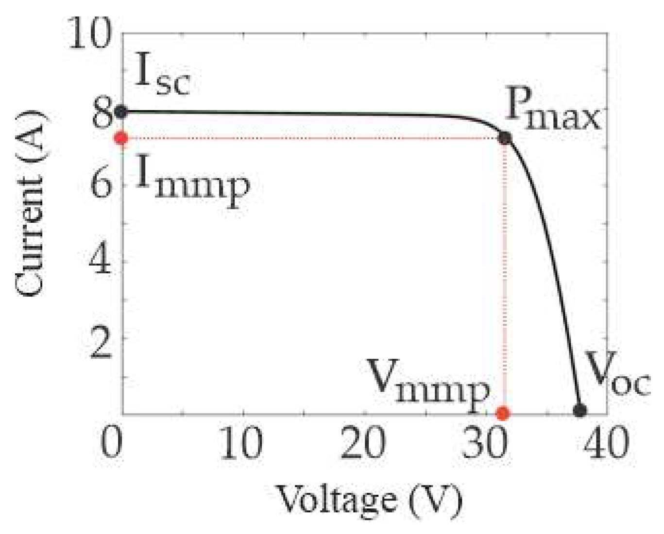
Figure 1. Typical PV module I–V curve with finite slopes near Isc (driven by Rsh) and near Voc (influenced by Rs and the diode term), consistent with the 1D5P model. The red dots indicate the short-circuit current (Isc), the maximum power point (Pmpp), and the open-circuit voltage (Voc). The red dotted lines highlight the current (Impp) and voltage (Vmpp) values at the maximum power point.
Processes 13 02999 g001
Figure 2. I–V curve for a shading fault.
Processes 13 02999 g002
Figure 3. Illustration of a CNN architecture. A, B, and C represent the number of filters, while a, b, and c denote the size of the filters.
Processes 13 02999 g003
Figure 4. Overview of the proposed methodology: (a) CNN design using simulated I–V curves; (b) classification process for unknown PV conditions.
Processes 13 02999 g004
Figure 5. Representative I–V curves corresponding to the four simulated operating conditions.
Processes 13 02999 g005
Figure 6. Simulink model of the photovoltaic module composed of three groups of 20 series-connected cells with bypass diodes.
Processes 13 02999 g006
Figure 7. Representation of the partial shading configurations for the four simulated conditions: (a) HLT, (b) LS, (c) MS, and (d) SS. Different shades of gray represent different irradiance levels.
Processes 13 02999 g007
Figure 8. Architecture of the CNN with a single convolutional layer.
Processes 13 02999 g008
Figure 9. Final CNN architecture with three convolutional layers.
Processes 13 02999 g009
Figure 10. Examples of different image sizes.
Processes 13 02999 g010
Figure 11. Accuracy and loss graphs. The circle highlights the final value of the training curve.
Processes 13 02999 g011
Figure 12. Confusion matrix for the final CNN configuration.
Processes 13 02999 g012
Figure 13. Grad-CAM visualizations for different PV module conditions: (a) HLT, (b) LS, (c) MS, and (d) SS.
Processes 13 02999 g013
Figure 14. Examples of I–V curves contaminated with different levels of white Gaussian noise: (a) 40 dB, (b) 30 dB, (c) 20 dB, and (d) 10 dB. Each subplot also includes Grad-CAM visualizations highlighting the CNN’s most relevant decision-making regions.
Processes 13 02999 g014
Figure 15. Classification accuracy of the CNN model under different noise levels.
Processes 13 02999 g015
Table 1. Performance of CNN configurations with a single convolutional layer. The green border highlights the best-performing value in the comparison.
Single LayerFilter Size
3 × 35 × 58 × 8
Number of filters492.1%92.9%93.1%
894.6%95.8%95.6%
1691.5%93.3%95.2%
3292.1%93.7%95.4%
Table 2. Performance of CNN configurations with two convolutional layers. The green border highlights the best-performing value in the comparison.
Two LayersFilter Size
3 × 35 × 58 × 8
Number of filters496.2%95.8%96.1%
896.9%96.0%96.2%
1695.6%96.0%95.9%
3296.2%94.7%96.1%
Table 3. Performance of CNN configurations with three convolutional layers. The green border highlights the best-performing value in the comparison.
Three LayersFilter Size
3 × 35 × 58 × 8
Number of filters496.4%97.1%97.1%
899.5%99.1%99.2%
1698.7%99.3%98.9
3296.0%97.5%98.1
Table 4. Classification accuracy for each image size. The green border indicates the highest-performing value in the comparison.
Image SizeAccuracy
51299.54%
25699.46%
12899.51%
6499.58%
3294.54%
Table 5. CNN settings.
Results
Validation accuracy99.5%
Training finishingMax epoch completed
Training cycle
Epoch10 of 10
Iteration700 of 700
Iteration per epoch70
Maximum iteration700
Validation
Frequency10 iterations
Other information
Hardware resourceSingle GPU
Learning rate scheduleConstant
Learning rate0.001
Activation functionsReLU and softmax
OptimizerAdam
Disclaimer/Publisher’s Note: The statements, opinions and data contained in all publications are solely those of the individual author(s) and contributor(s) and not of MDPI and/or the editor(s). MDPI and/or the editor(s) disclaim responsibility for any injury to people or property resulting from any ideas, methods, instructions or products referred to in the content.