Abstract
Emerging power electronic devices like soft open points (SOPs) and electric springs (ESs) play a vital role in enhancing active distribution network (ADN) efficiency. SOPs enable flexible active/reactive power control, while ESs improve demand-side management and voltage regulation. This paper proposes a two-stage stochastic programming model to optimize ADN’s operation by coordinating these fast-response devices with legacy mechanical equipment. The first stage determines hourly setpoints for conventional devices, while the second stage adjusts SOPs and ESs for intra-hour control. To handle ES nonlinearities, a hybrid data–knowledge approach combines knowledge-based linear constraints with a data-driven multi-layer perceptron, later linearized for computational efficiency. The resulting mixed-integer second-order cone program is solved using commercial solvers. Simulation results show the proposed strategy effectively reduces power loss by 42.5%, avoids voltage unsafety with 22 time slots, and enhances 4.3% PV harvesting. The coordinated use of SOP and ESs significantly improves system efficiency, while the proposed solution methodology ensures both accuracy and over 60% computation time reduction.
1. Introduction
With the global shift toward renewable energy and the collective commitment to carbon neutrality, the installation of distributed renewable generators has been accelerating at an unprecedented rate. According to data from the International Renewable Energy Agency [1], 585 GW of renewable energy capacity was added worldwide in 2024, with China accounting for approximately 63.8% of this total. At the distribution grid level, projections suggest that by the end of 2025, China could deploy over 500 GW of renewable generators and more than 120 million charging infrastructure units to support its 2060 carbon neutrality target [2]. This transition from fossil fuels to cleaner, distributed energy sources presents both opportunities and challenges for the dynamic operation of power distribution networks. Meanwhile, the inherent uncertainty and variability of renewable energy, particularly widely adopted photovoltaic (PV) systems, pose significant challenges to voltage regulation, power loss reduction, and overall system efficiency. Consequently, traditional passive distribution networks are being reconfigured into active distribution networks (ADNs), which incorporate real-time monitoring [3], intelligent dispatch [4], and flexible control enabled by advanced power electronic interfaces and distributed energy resources (DERs).
In this context, enhancing operational efficiency has become a critical objective for the secure and economic operation of ADNs. Efficient operation not only ensures the optimal utilization of renewable resources and controllable assets such as on-load tap changers (OLTCs) and capacitor banks (CBs) but also supports the network in maintaining fine regulation under uncertain operating conditions [5]. To address the operational challenges introduced by stochastic-generated renewable energy while maintaining system efficiency, power-electronics-based technologies have been increasingly explored in recent years. Among them, soft open points (SOPs) and electric springs (ESs) have emerged as two promising solutions for enhancing the operational efficiency of ADNs.
A SOP is a power electronic device that replaces traditional mechanical tie-switches at normally open points in distribution networks [6], as shown in Figure 1. Both terminals of SOP are voltage source converters (VSCs), and are decoupled by the DC capacitance. Owing to the DC isolation, each terminal of SOP can be controlled independently, thus enabling fast and continuous control of active and reactive power flow between two terminals, improving voltage profiles, reducing network losses, and facilitating higher DER penetration. Preliminary studies have investigated the application of SOPs in distribution system operation. For instance, ref. [7] integrates SOPs to enhance voltage stability and reduce losses, while the author of [8] employs SOP for imbalance mitigation in ADNs. In [9], a coordinated control strategy between SOPs and energy storage systems is proposed to improve operational flexibility. Under normal operating conditions, SOPs have demonstrated effectiveness in network reconfiguration and optimal power flow management [10]. Furthermore, stochastic and robust optimization techniques have been applied to optimize SOP placement and operation under renewable generation uncertainty [11,12,13].
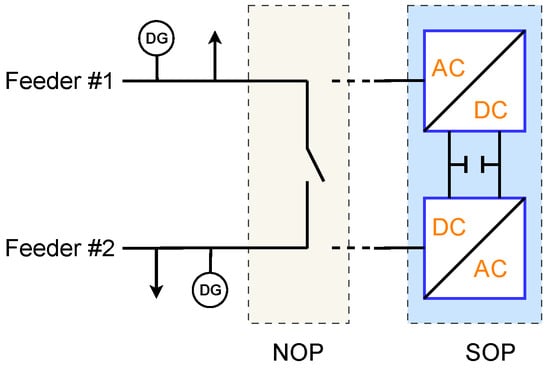
Figure 1.
Schematic diagram of SOP installation in distribution network.
ES is an advanced power electronics apparatus deployed on the demand side, installed between a distribution bus and non-critical loads (NLs). The main structure of ES is a voltage source inverter (VSI), making it both cost-effective and highly responsive in voltage and reactive power control, as shown in Figure 2. Unlike conventional compensators, the ES exclusively regulates reactive power, eliminating the need for costly active power converters [14]. When combined with NLs, the series structure forms a smart load (SL), operating in parallel with critical loads (CLs) to enhance grid efficiency [15]. In ADN with ESs, NLs refer to electric loads that can undertake relatively wide voltage and power variations. On the other hand, CLs require a stable power and voltage supply. By adjusting the voltages of ESs and NLs, ESs can provide real-time voltage support and absorb surplus renewable energy. This makes ES particularly suitable for applications in systems with high penetration of distributed PV units. The concept was first introduced in [16], where the fundamental operating principle and circuit topology were established. Since then, various control strategies have been developed to improve ES performance. Droop and distributed control methods are proposed in [17,18] for voltage regulation in low-voltage networks with high PV integration. In [19], ESs are utilized to improve ADNs’ efficiency through loss reduction and voltage flattening. Additional benefits of ESs include enhanced system flexibility [20], resilience [21], imbalance mitigation [22], and frequency support [23].
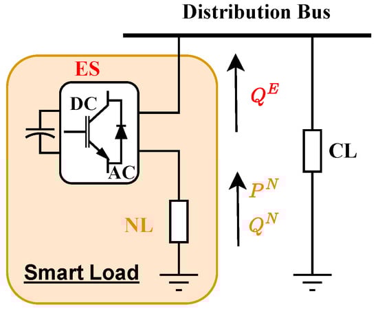
Figure 2.
Schematic diagram of ES installation in distribution network.
While both SOPs and ESs contribute to voltage regulation and operational efficiency, they operate at different levels of the distribution system: SOPs act at the network level by controlling inter-feeder power flows, whereas ESs function at the demand side by modulating end-user load consumption. Existing studies typically treat SOPs and ESs in isolation, with limited focus on their coordinated operation across multiple timescales under stochastic renewable generation. Therefore, to bridge this gap, this paper proposes a two-stage stochastic coordination framework that jointly dispatches SOPs and ESs to enhance ADN operational efficiency while accounting for uncertainties. The key contributions are summarized as follows:
- A two-stage stochastic programming model is proposed to enhance operational efficiency in ADNs with hourly and intra-hour timescale coordination control. The model accounts for uncertainties in PV output and load demand to improve solution robustness. The hourly-stage control is realized by operating legacy mechanical devices (OLTC and CB) as “here-and-now” first-stage actions. The intra-hour stages are realized by joint dispatch of SOPs and ESs to act as “wait-and-see” second-stage actions to compensate for the first-stage solutions.
- A computationally efficient solution methodology that convexifies non-convex power flow and SOP capacity constraints, while employing a data–knowledge hybrid-driven approach for ES modeling is proposed. A multi-layer perceptron (MLP) learns the nonlinear ES operational characteristics and is subsequently linearized using mixed-integer programming. Finally, the optimization problem is reformulated into a tractable mixed-integer second-order cone programming model (MISOCP) that can be handled reliably and efficiently with commercial solvers.
Numerical simulations are conducted based on the IEEE 33-bus distribution system, revealing that the proposed two-stage stochastic coordination strategy effectively enhances the operational efficiency of ADNs. The hybrid solution methodology reduces computational burden while maintaining high solution accuracy.
The rest of the paper is organized as follows: Section 2 gives the problem formulation, organized into a two-stage stochastic programming model. Section 3 details the solution methodology. The case study in Section 4 validates the proposed approach. Lastly, Section 5 finalizes this paper with conclusions.
2. Problem Formulation
2.1. Objective and System Modeling
2.1.1. Objective Function
ADN is designated to deliver power to electric loads in the network, requiring high efficiency on power delivery and high-quality voltage regulation. To enhance operational efficiency, we formulate the optimization problem comprising two key ideas: minimizing active power losses and flattening bus voltage profiles, as follows:
where and are weighting parameters; and are resistance and squared magnitude of the current through branch ; and is the duration of the decision time slot. and are non-negative slack variables representing upper voltage violation and lower voltage violation, respectively. corresponds to the objective of reducing total power loss to improve power delivery efficiency. In contrast, quantifies the cumulative voltage deviation from a desired control range, and is defined via soft constraints with slack variables, as given in (2)–(4).
For instance, when the bus voltage lies within the desired control threshold , slack variables and are zero, indicating no violation. However, if the voltage exceeds this range, the corresponding slack variable becomes positive, quantifying the deviation. Note that the calculation of voltage deviation takes the squared magnitudes for a better link to the power flow modeling.
2.1.2. Modeling of Active Distribution Network
The DistFlow model [24] is often leveraged to describe radial distribution networks:
where and denote active and reactive power injection in bus j and time t, respectively. and denote the active and reactive power through the branch at time t, respectively. The branch set with is defined to describe the topology of the network, which consists of buses. The subscript denotes that bus k is one of the son nodes of bus j in the radial network. The bus voltage and line current are determined by and , respectively. Equations (5) and (6) present the nodal and branch power relationship. Equations (7) and (8) give the calculation of bus voltage and line current, respectively.
Equations (9) and (10) present the active power and reactive power injection at each bus, respectively. represents the active power generated by PV arrays at bus j and time t. represents the reactive power compensation from CB at bus j and time t. and represent the active power output of SOP and active power demand of electric loads, respectively. and represent the reactive power output of SOP and the reactive power demand of electric loads, respectively. and represent the active and reactive power demand of ES-based smart load, respectively.
2.1.3. Modeling of Legacy Devices
Grid-owned legacy devices are incorporated for the regulation services. Constraints (11)–(13) correspond to the modeling of OLTC, and constraints (14) and (15) correspond to the modeling of CB.
Constraint (11) denotes the voltage of the bus with OLTC connection. represents the base voltage of bus j; is the squared value of OLTC tap positions, and is calculated via Equation (12); and and represent the minimum tap position and the difference between each tap position, respectively. The binary variable indicates whether the s-th tap of the OLTC at bus j is active at time t. For instance, for an OLTC with ten taps and voltage regulation function, is 0.95 p.u. and is 0.1 p.u. Logic constraint (13) ensures proper action of OLTC taps, guaranteeing that the tap position does not exceed the maximum tap number .
Constraint (14) denotes the reactive power compensated by CB at bus j and at time t. denotes the reactive power capability of each CB step unit, and the binary variable denotes the on/off status of the s-th CB unit. Similarly to (13), logic constraint (15) ensures the proper function of each CB step unit.
2.1.4. Modeling of SOP
In distribution networks, especially large-scale distribution networks, the loss of SOP is relatively negligible compared to the overall system losses; therefore, this work does not consider the loss of SOP. So the active power balance between SOP terminals can be governed as in (16). For reactive power compensation, each terminal of the SOP operates independently within its respective capacity limits [25], as in (17) and (18).
Additionally, the apparent power at both terminals must comply with the SOP’s total capacity limitation, as follows:
2.1.5. Modeling of ES
As the penetration of ESs increases across distribution networks, their collective regulation capability significantly improves grid performance. Based on the derivation in [19], the ES voltage and power regulation effect characteristics are modeled as follows:
where Equation (21) corresponds to the voltage regulation effect of ES; Equation (22) and Equation (23) represent the active and reactive power demand of the ES-based SL, respectively; and represent the voltage and impedance of the NL; denotes the power factor of the NL; and the reactive power compensation from ES is . Note that in Equation (22), the active power of SL is the same as the active power of NL since ES purely compensates reactive power.
Furthermore, to ensure operational safety, the voltage of the NL must stay within its permissible variation limits, and the output of the ES must not exceed its capacity constraints, as follows:
2.1.6. System Operation Constraints
To ensure safe operation of ADN, nodal voltage constraints and line thermal constraints have to be considered in the optimization model formulation, as follows:
where and correspond to the lower and upper safe limit for bus voltage, respectively; corresponds to the thermal limit of the distribution branch.
The imported active and reactive power from the upper transmission grid must satisfy the capacity limits of the substation node to avoid overloading of ADN, as follows:
where and refer to the active and reactive power at the substation node, respectively.
2.2. Proposed Two-Stage Stochastic Coordination Strategy
For practical operation, the increasing penetration of renewable energy generation, particularly distributed PV, introduces significant operational challenges for distribution networks due to the inherent variability and uncertainty of their power output. As described in Equation (30), the actual PV power output may deviate from its forecast by an uncertain term , which follows a zero-mean Gaussian distribution with variance :
Similarly, load demand may also deviate from its forecast . These stochastic fluctuations can cause rapid voltage variations, which conventional mechanical devices (OLTC and CB) are unable to mitigate due to their slow and discrete response, potentially degrading network performance and operational efficiency [26]. In contrast, as state-of-the-art power electronic devices, SOPs and ESs offer fast, continuous control, enabling voltage regulation.
To leverage the complementary strengths of legacy mechanical devices and fast-responding power electronics, this paper proposes a two-stage stochastic coordination framework, as illustrated in Figure 3. The conventional hourly operation period is divided into four 15-minute intervals, establishing a two-timescale coordination strategy: long-term (1 h) for OLTC and CB dispatch and short-term (15 min) for SOP and ES control. The long-timescale decisions (OLTC taps, CB switching) are treated as first-stage (“here-and-now”) variables, fixed for the entire hour. The short-timescale responses (SOP active/reactive power output, ES reactive support) are second-stage (“wait-and-see”) actions, adjusted dynamically to compensate for intra-hour uncertainties. The overall problem is formulated as a two-stage stochastic program, as follows:
where is the deterministic cost of the first-stage decision; is the stochastic cost of second-stage decisions; u denotes the first-stage decisions in the feasible set ; and represent second-stage decisions under uncertainty data , constrained to the set . The second-stage problem is defined as: , where denotes the objective of the second-stage problem. The first-stage decision u is made before the actual realization of the random variable . The second-stage decision is made after is observed to compensate for the first-stage decision as a recourse action.
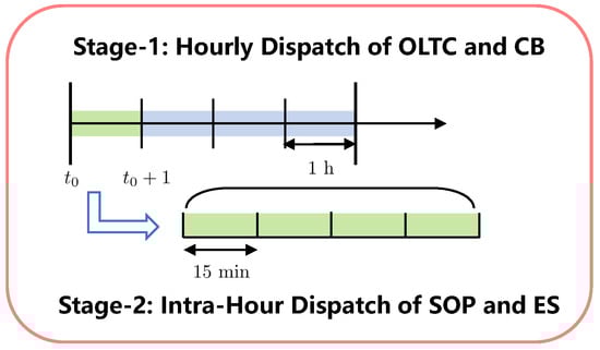
Figure 3.
Proposed two-stage stochastic coordination framework.
The constraint refers to the feasible set that determines the first-stage solution, while the constraint set refers to the feasible set that determines the second-stage solutions with optimized first-stage solutions, as follows:
By far, the proposed optimization problem is modeled as a two-stage stochastic programming model, enabling coordinated control across timescales to address both hourly trends (via OLTC and CB) and intra-hour fluctuations(via joint dispatch of SOPs and ESs).
3. Solution Methodology
The inclusion of nonlinear constraints for SOP (19) and (20) and ESs (21) and (22), alongside the non-convex power flow constraints (8), renders the optimization model (31) a computationally intensive mixed-integer nonlinear program (MINLP) with non-smooth expectations. To address this computational burden, we propose a hybrid strategy that ultimately allows the two-stage stochastic programming problem to be cast as an MISOCP model, enabling efficient solution via commercial optimization software.
3.1. Convexification of Constraints
The non-convex power flow constraint (8) is an equality constraint and has been shown in [27] that it can be relaxed into an inequality form that maintains exactness provided certain mild conditions are met, as follows:
3.2. Data-Driven Modeling for ES
3.2.1. Variable Substitution
Before laying out the data-driven method for replicating the nonlinear ES model, we first substitute the voltage of NL with its squared value such that the nonlinear dimension of original ES modeling and constraints can be reduced. The voltage constraint for ES, originally Equation (21), can be reformulated as follows:
The active power of SL can be represented as follows:
Meanwhile, the voltage tolerance of NL is replicated with its squared form, as follows:
Then, the modeling and constraints for ES application are composed of refined ES voltage constraints (38), refined SL active power constraints (39), SL reactive power constraints (23), refined NL voltage tolerance constraints (40), as well as ES capacity constraints (25). Thus, ES modeling is reformulated into a set of linear constraints and a nonlinear constraint (38).
3.2.2. Data-Driven MLP
Due to the existence of the nonlinear constraint (38), the computation cost of (31) is still high, and the guarantee of optimality is still hindered. Herein, we propose a data-driven method to replicate the refined nonlinear ES voltage constraint (38).
The MLP, as a feed-forward neural network, is capable of capturing intricate input–output relationships through hierarchical transformations. As shown in Figure 4, the MLP is typically made up of one input layer, multiple hidden layers, and one output layer. The input layer receives the input feature vector, the hidden layers transform inputs via learnable weights and an activation function (usually nonlinear), e.g., ReLU, and then, the output layer produces the final prediction. The depth and width of the network are two key architectural dimensions that govern the approximation capability of MLP [28].
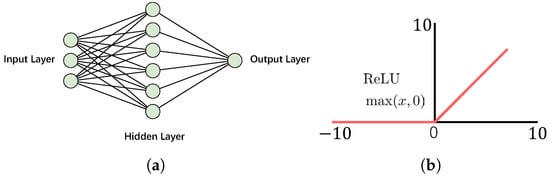
Figure 4.
(a) Structure diagram of an MLP. (b) Activation function of ReLU.
The input vector and output for the MLP network of ES are defined as follows:
Then, the regression procedure maps from input to output, as follows:
where and represent the output of the -th layer and n-th layer, respectively. represents the linear mapping result of each layer. represents the final output of the MLP. For each layer of the MLP, and are learnable parameters to be trained, which signify the weighting matrix and bias vector of the n-th layer, respectively.
As per the MLP trained for ES, Equations (41) and (42) define the input and output layers. Equations (43)–(45) describe its internal operations. Crucially, both the inputs and outputs of this MLP align with the controllable variables within the established optimization model. Consequently, a well-trained MLP can effectively approximate the nonlinear ES voltage constraint (38) with high accuracy.
3.2.3. MLP Reformulation
Despite the fact that the trained MLP model (41)–(45) for ES exhibits low nonlinearity and proves highly practical, the computational complexity of the optimization problem (31) remains substantial. This difficulty stems from the inherent non-convexity introduced by the ReLU activation functions in (44). Herein, we introduce a set of binary variables , a set of auxiliary variables , and a sufficiently large positive constant M to linearize the nonlinear constraints [29]:
Note that Equation (46) replaces the original linear mapping Equation (43), while constraints (47) and (48) serve as linear approximations of the ReLU activation function (44). This reformulation enables the representation of the ES models using linear physical constraints set {(23), (25), (39), (40)} and a linearized data-driven MLP model {(41), (42), (45), (48)}, thereby facilitating more efficient optimization and analysis.
3.3. Problem Reformulation
After convexifying the constraints and employing data-driven modeling for ES, all nonlinear and non-convex constraints have been reformulated into tractable formulas. Then, with forecast data and the probability distribution functions of PV output and load demand, the scenario method can be deployed to handle the two-stage stochastic programming problem, as follows:
where denotes the probability mass of scenario . Refined first-stage decision constraints set (50) and refined second-stage decision constraints set (51) are defined as follows:
4. Case Study and Analysis
The case study is conducted on the modified IEEE 33-bus test system, as illustrated in Figure 5a. An OLTC is connected at the substation node with a 10% voltage regulation range. A CB with 300 kVar reactive power compensation capability is installed at bus 25. Five 700 kW PV plants are integrated into the network. Two SOPs, each rated at 500 kVA (with 300 kVar reactive power capability), are placed between buses 11 and 21. Eight ESs are distributed across the system. NLs and CLs are assumed in a 70:30 ratio [30], with NLs tolerating up to 10% voltage variation as per (40). Note that the load is predefined and remains constant, regardless of voltage changes. The objective function weights are set to 0.833 and 0.167 for the respective terms. The prediction errors of PV and load demand follow the Gaussian distribution with standard deviations of 10% and 5%, respectively. A total of 1000 Monte Carlo scenarios are generated and reduced to 20 representative scenarios using a distance-based reduction method. Table 1 presents the remaining parameters. Figure 5b shows the 15-minute profiles of the PV output and load demand in the test system. The nominal power of the load is predefined and remains constant irrespective of voltage fluctuations. Consequently, the actual load is determined by multiplying the nominal power by the load ratios provided in Figure 5b.
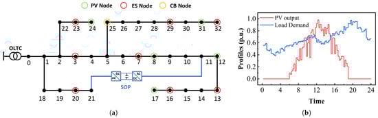
Figure 5.
(a) The modified IEEE 33-bus test system. (b) The 15 min profiles of PV output and load demand.

Table 1.
Parameter setup.
The training dataset for the ES voltage constraints is generated using the full ES model. Specifically, voltage pairs are randomly sampled within the bounds defined by the NL voltage constraint (24) and the system voltage limit (26). These voltage pairs, along with the load impedance angle , are input to the ES voltage equation (21) to compute the corresponding reactive power output . Over 10,000 feasible data samples are collected for training and testing the ES MLP model. During generation, any sample violating the ES capacity constraint (25) is discarded to ensure feasibility.
The optimization model is gathered with CVXPY 1.7 and solved with Gurobi 12.0. The regression MLP is constructed using PyTorch 2.7.1 with a batch size of 128 and 600 epochs. All numerical experiments are conducted on an Intel (R) i5-10210U 1.6 GHz CPU with 16 GB of memory.
4.1. Regulation Performance
First, the regulation performance of the proposed two-stage stochastic coordination strategy is evaluated by comparing it with two benchmark cases: (1) an ADN without any regulation schemes and (2) an ADN employing only hourly dispatch of OLTC and CBs. Figure 6 illustrates the voltage profiles across the test system under these different cases, where red and blue dashed lines refer to the safe and flattening limits, respectively.
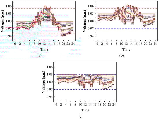
Figure 6.
Voltage profiles under different scenarios. (a) ADN without regulation. (b) ADN with hourly regulation of OLTC and CB. (c) ADN with the proposed two-stage stochastic coordination strategy.
As shown in Figure 6a, in the absence of regulation, bus voltages violate both the safe upper limit during periods of high PV generation and the lower limit during peak demand periods. This highlights significant voltage security challenges in unregulated ADN operations. When hourly dispatch of OLTC and CB is applied, as in Figure 6b, voltage violations—particularly at the lower (safe and flattening) bounds—are significantly mitigated, showing high voltage quality. This improvement arises because the OLTC maintains a higher secondary-side voltage during peak load periods, supporting voltage levels across the network. However, during peak generation periods, due to the intermittent and stochastic nature of PV generation within intra-hour intervals, the fixed-hourly OLTC and CB settings cannot adapt dynamically, limiting their ability to suppress overvoltages during rapid PV output fluctuations. Moreover, the constant reactive power injection from CBs can lead to overcompensation during periods of reduced load or high PV output, resulting in intra-hour overvoltage violations. It is worth noting that control of OLTC and CB creates a foundational platform for the second-stage operation of SOPs and ESs. Notably, in the absence of regulation, there are 21 instances of 15 min violations of 56 violations of flattening limits. With Stage 1 alone, these violations are reduced to 41, representing a reduction of 26.8%. This improvement underscored the critical contribution of Stage 1 to voltage flattening.
Figure 6c shows the voltage profiles of the test system based on the proposed approach, demonstrating that the two-stage stochastic coordination framework effectively leverages SOPs and ESs for intra-hour regulation on a 15 min timescale, complementing the hourly OLTC/CB actions. Under this strategy, all bus voltages remain strictly within the prescribed safety limits—neither exceeding the upper bound nor falling below the lower bound. Furthermore, the secondary objective , which promotes voltage flattening, ensures that all node voltages are maintained within ±3% of the nominal value. This tight regulation reflects a high degree of voltage quality control and demonstrates the strategy’s capability to achieve not only voltage security but also superior voltage stability and quality.
Figure 7 presents a comparison of power losses in the test network under different operational scenarios. As shown, power loss reaches its peak during high-demand periods due to heavy loading on the distribution lines. Similarly, during periods of peak PV generation, reverse power flow can also lead to increased losses. In the absence of any regulation, power losses are the highest across all time intervals, exceeding those observed under both the hourly regulation scheme and the proposed two-stage strategy. Both during peak demand and peak generation periods, the proposed strategy achieves the lowest power loss. Moreover, throughout the remaining operating periods, it consistently maintains lower losses compared to the other cases.
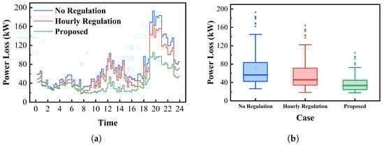
Figure 7.
(a) Power loss in the networks under different scenarios. (b) Statistical analysis of power loss.
As shown in Figure 7b, in the unregulated case, the maximum, minimum, and average power losses reach 193.1 kW, 26.3 kW, and 71.3 kW, respectively, resulting in a total power loss of 1710.4 kWh over 24 h. Such high losses significantly reduce system efficiency, leading to higher operational costs. With hourly regulation by OLTC and CB, losses are reduced to 164.0 kW (maximum), 18.4 kW (minimum), and 59.8 kW (average), yielding a total loss of 1435.2 kWh, which is a reduction of 16.1% compared to the unregulated case. This demonstrates that hourly control can effectively help to mitigate losses, not only improving operational efficiency but also setting the stage for further loss minimization in Stage 2, which highlights the synergistic effect between the two stages and greatly contributes to the ADN operation.
However, the proposed two-stage stochastic coordination strategy further reduces the maximum, minimum, and average power losses to 104.5 kW, 17.3 kW, and 41.0 kW, respectively. The total power loss is reduced to 983.5 kWh, representing a 42.5% reduction compared to the unregulated case and a 31% reduction compared to hourly regulation. This substantial improvement highlights the superior operational efficiency enabled by the proposed strategy.
4.2. Comparative Analysis
Then, we conduct a comparative analysis to demonstrate the advantages of two-stage stochastic coordination over a single-stage strategy, and another comparative analysis to demonstrate the benefit of joint dispatch over independent dispatch of SOP or ES.
4.2.1. Comparison with Single-Stage Strategy
The proposed strategy in (49) is a two-stage stochastic programming model that explicitly accounts for intra-hour uncertainties in PV output and load demand. It leverages the fast response capabilities of ESs and SOP to mitigate rapid fluctuations within each hour. In contrast, the single-stage strategy neglects the expectation term in (49), thereby ignoring intra-hour uncertainties in the decision-making process. As a result, the dispatch of OLTC, CB, SOP, and ES remains fixed throughout the hour, and ESs and SOPs are not dynamically adjusted in real time.
Figure 8 illustrates the voltage profiles of the test system under 200 random scenarios (generated via Monte Carlo simulation) from 13:00 to 14:00, where red and blue dashed lines refer to the safe and flattening limits, respectively. Since the single-stage strategy does not account for potential intra-hour variations in load and PV generation, it adopts a riskier operating point: the secondary-side voltage of the OLTC is set to 1.01 p.u., and the CB provides a fixed reactive power compensation of 300 kVar. Consequently, the maximum bus voltages approach the voltage flattening upper bound of 1.03 p.u. Without adaptive adjustment from ESs and SOPs, approximately 8.5% of the scenarios exceed the safety limit (1.05 p.u.), and around 45% violate the flattening limit (1.03 p.u.), demonstrating that the single-stage approach fails to handle intra-hour variability due to its neglect of uncertainty.
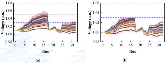
Figure 8.
Voltage profiles of different strategies under random scenarios. (a) Single-stage strategy. (b) Proposed two-stage stochastic coordination strategy.
In stark contrast, the proposed two-stage stochastic coordination strategy incorporates second-stage uncertainty realizations into the first-stage decisions, resulting in a more conservative and robust solution. It sets the OLTC secondary voltage to 1.00 p.u. and the CB compensation to 200 kVar, thereby reducing the initial voltage stress. Under random scenarios, ESs and SOP adaptively respond to intra-hour fluctuations based on real-time monitoring, ensuring that all bus voltages remain within both the safety bounds (0.95–1.05 p.u.) and the tighter flattening bounds (0.97–1.03 p.u.).
It can be concluded that the single-stage strategy fails to fully exploit the fast response characteristics of power electronic devices and does not consider intra-hour uncertainties, leading to significant voltage violations during the hour. In contrast, the proposed two-stage stochastic programming model integrates the potential realizations of second-stage uncertainties, significantly enhancing regulation performance and operational robustness. The hourly dispatch of OLTC and CB establishes a robust foundation for the intra-hour control actions conducted by SOPs and ESs in Stage 2. This conservative first-stage solution significantly supports the intra-hour adjustments, ensuring that uncertainties are effectively managed. By enabling ESs and SOPs to rapidly adapt to intra-hour variations, their dynamic response capabilities are fully utilized, greatly contributing to operational efficiency enhancement in ADNs.
4.2.2. Benefit Analysis on Joint Dispatch of SOP and ES
The benefit brought by the joint dispatch of SOP and ES on enhancing the operational efficiency of ADN is analyzed by comparing it with two different schemes. The hourly dispatches are all conducted by the OLTC and CB, while the following schemes realize the second-stage (intra-hour) dispatches:
- Scheme A:
- Intra-hour regulation solely based on SOP.
- Scheme B:
- Intra-hour regulation solely based on ESs.
- Scheme C:
- Intra-hour regulation based on joint dispatch of SOP and ESs (proposed).
Scheme A and Scheme B correspond to the optimization problem in (49) without ESs and without SOP, respectively. In contrast, the proposed Scheme C utilizes the full model, incorporating both SOP and ESs. The voltage violation ratio is computed as the total duration of violations divided by the overall simulation time.
As shown in Table 2, relying solely on hourly regulation via OLTC and CB results in voltage violations exceeding the safety limit for 9.3% of the time, posing significant risks to system security. Although Scheme A reduces these violations to 6.2%, it still fails to eliminate them entirely and cannot meet the stricter voltage flattening requirement, which remains violated for 12.5% of the time. In contrast, Scheme B, utilizing eight distributed ESs, completely eliminates both safety and flattening limit violations. This superior performance can be attributed to the spatial flexibility and rapid response capabilities of distributed ESs, which offer greater regulation flexibility compared to a single SOP. Then, with the joint dispatch of eight ESs and SOP (proposed Scheme C), voltage regulation performance remains excellent, with zero voltage violations under both criteria and all bus voltages kept within the desired flattening bounds at all times.
Table 2.
Comparison of regulation schemes for the modified IEEE 33-bus Test System.
Regarding network power losses, Scheme A and Scheme B achieve reductions of 10.95% and 18.12%, respectively, compared to the hourly-only scheme. In contrast, the proposed joint dispatch reduces losses by 31.47%, significantly outperforming both Scheme A and Scheme B. This indicates that coordinating ESs and SOP yields lower power loss than relying solely on either device alone.
Compared to Scheme A, which solely depends on SOP for intra-hour regulation, the proposed scheme considers ESs for cooperation, thus realizing no voltage violations and lower losses. Compared to Scheme B, which solely depends on ESs for intra-hour regulation, the proposed scheme incorporates SOP for cooperation, thus achieving even lower power loss. Overall, the proposed joint dispatch scheme outperforms both Scheme A and Scheme B. The joint dispatch of SOP and ES not only ensures operational safety but also significantly enhances the overall operational efficiency of ADNs. It demonstrates superior performance in both voltage regulation and power loss reduction compared to using SOP or ES independently.
In conclusion, the above comparative analyses demonstrate that the proposed two-stage stochastic coordination strategy significantly improves intra-hour voltage regulation, ensures operational robustness, and minimizes power losses while maintaining zero voltage violations. By leveraging the fast response capabilities of SOP and ESs to complement the slower OLTC and CB actions, the strategy effectively bridges temporal gaps in control. This synergistic coordination paves the way for more reliable and efficient management of ADNs.
4.3. Algorithm Validation
Further, this section gives validation for the proposed solution algorithm from two perspectives: the performance of the trained MLP in characterizing ES and the computational efficiency of the reformulated MISOCP model.
The MLP is trained offline using collected operation data and is used to approximate the nonlinear ES voltage constraints. In this study, we employ a shallow MLP architecture consisting of 3 neurons in the input layer, 15 neurons in a single hidden layer, and 1 neuron in the output layer. Training is performed using the stochastic gradient descent (SGD) optimizer on a standard CPU. The average training time is approximately 50 s, which is negligible in the context of offline model development. Figure 9 illustrates the training loss and prediction accuracy of the MLP. As shown, the training loss decreases rapidly and converges to a small value, indicating effective learning. Figure 9b presents the prediction errors for both capacitive and inductive operating modes of the ES. The maximum prediction errors are below 0.8 kVar, while the average errors do not exceed 0.2 kVar for either mode. These results demonstrate that the trained MLP accurately captures the nonlinear operational characteristics of ESs, enabling high-fidelity representation within the optimization framework. Given the high accuracy achieved with such a lightweight network, the overall complexity of the data-driven MLP is very low.
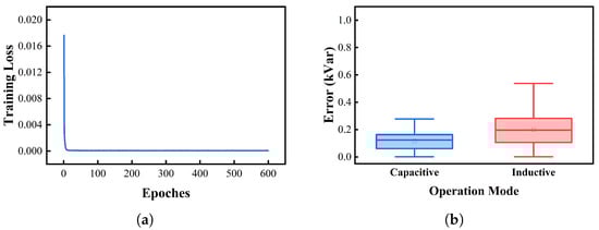
Figure 9.
(a) Training loss of the MLP. (b) Prediction errors of the MLP in characterizing ES of capacitive mode and inductive mode.
By replicating the ES nonlinear constraint with the well-trained MLP and applying convexification techniques to the power flow and SOP constraints, the original MINLP problem is reformulated as a tractable MISOCP. This reformulated model is solved using the commercial solver Gurobi. For comparison, the original MINLP is solved using two approaches: (1) the BARON solver, which employs a duality-based branch-and-bound algorithm for the MINLP model; (2) Gurobi’s built-in spatial branching method with outer approximation, which is a global optimization method [31].
MINLP is generally NP-hard and requires exponential time in the worst case. The global optima of MINLP cannot be guaranteed. As shown in Table 3, due to the presence of multiple scenarios, inherent nonlinearity, and non-convexity, BARON fails to converge and returns an infeasible solution, highlighting the computational difficulty of the original MINLP formulation. Gurobi’s spatial branching method successfully obtains a solution within 275 s, providing a globally optimal approximation of MINLP.
Table 3.
Convergence and solving efficiency of different methods.
In contrast, even though the MISOCP problem is still NP-hard in general, it is known to be polynomially solvable in the case of convex problems if all nonlinear constraints are second-order cone representable. Based on the modern branch-and-bound method and accelerating methods, the MISOCP empirically has better scalability than the MINLP solution. The structured convexity enables MISOCP frameworks to grow polynomially with problem size, while MINLP often exhibits exponential growth in runtime due to the challenges of exploring nonlinear and non-convex solution spaces. As shown in Table 3, the proposed MISOCP approach achieves convergence in only 101.2 s, with an average deviation of just 0.1% from the reference global objective value obtained by Gurobi. This represents a reduction in computation time of over 60%, while maintaining extremely high solution accuracy. These results demonstrate that the proposed methodology significantly alleviates the computational burden and ensures robust convergence, making it highly effective for solving the two-stage stochastic coordination strategy in ADNs. The computational convergence also demonstrates the lower complexity of MISOCP over MINLP, improving tractability compared to solving the original MINLP directly.
Overall, the proposed MISOCP solution with linearized MLP demonstrates significantly reduced computational complexity, allowing the use of off-the-shelf solvers with improved tractability compared to solving the original MINLP directly.
5. Conclusions
This paper presents a two-stage stochastic coordination approach to enhance the operational efficiency of ADNs by optimizing legacy mechanical devices with joint dispatch of SOPs and ESs. The proposed framework optimizes hourly setpoints for conventional devices in the first stage, while SOPs and ESs provide intra-hour adjustments to mitigate fluctuations in the second stage. To address the nonlinearities in ES modeling, a hybrid data–knowledge methodology is employed, integrating knowledge-based linear constraints with a data-driven MLP model, which is subsequently linearized for computational efficiency. The resulting MISOCP formulation ensures tractable and reliable optimization. Simulation results demonstrate that the proposed strategy effectively reduces power losses, mitigates voltage violations, and enhances renewable energy integration. The coordinated operation of SOPs and ESs significantly improves system efficiency and responsiveness. Compared to the single-stage strategy, the proposed strategy enhances the solution robustness of intra-hour regulations. The hybrid modeling approach maintains high computational accuracy with reasonable solver times. Future work will investigate the scalability of this method for larger distribution networks and more efficient methods for reducing the number of binary variables.
Author Contributions
Conceptualization, L.C. and J.G.; methodology, L.C., J.G. and L.L.; software, L.C.; validation, L.C., J.G. and K.-W.L.; formal analysis, K.-W.L. and L.W.; investigation, L.L.; writing—original draft, J.G. and L.W.; writing—review and editing, L.C. and L.W.; supervision, K.-W.L.; project administration, K.-W.L. and L.W. All authors have read and agreed to the published version of the manuscript.
Funding
This research was supported by the National Natural Science Foundation of China (62001169) and the Guangdong 2025 Basic and Applied Basic Research Project (SL2024A04J01736).
Data Availability Statement
The raw data supporting the conclusions of this article will be made available by the authors on request.
Conflicts of Interest
The authors declare no conflicts of interest.
References
- Saeed, S.; Siraj, T. Global Renewable Energy Infrastructure: Pathways to Carbon Neutrality and Sustainability. Sol. Energy Sustain. Dev. J. 2024, 13, 183–203. [Google Scholar] [CrossRef]
- Jin, Y.; Zhang, S.; Sarkis, J.; Zhao, J. Multiple Roads to Carbon Neutrality in China. IEEE Eng. Manag. Rev. 2025, 53, 12–16. [Google Scholar] [CrossRef]
- Lin, J.; Wan, C.; Song, Y.; Huang, R.; Chen, X.; Guo, W.; Zong, Y.; Shi, Y. Situation awareness of active distribution network: Roadmap, technologies, and bottlenecks. CSEE J. Power Energy Syst. 2016, 2, 35–42. [Google Scholar] [CrossRef]
- Zhao, J.; Wu, Z.; Long, H.; Sun, H.; Wu, X.; Chan, C.; Shahidehpour, M. Optimal Operation Control Strategies for Active Distribution Networks Under Multiple States: A Systematic Review. J. Mod. Power Syst. Clean Energy 2024, 12, 1333–1344. [Google Scholar] [CrossRef]
- Yu, Q.; Wang, Q.; Li, W.; Liu, F.; Shen, Z.; Ju, J. Two-Layer Collaborative Architecture for Distributed Volt/Var Optimization and Control in Power Distribution Systems. IEEE Access 2019, 7, 173344–173357. [Google Scholar] [CrossRef]
- Jiang, X.; Zhou, Y.; Ming, W.; Yang, P.; Wu, J. An overview of soft open points in electricity distribution networks. IEEE Trans. Smart Grid 2022, 13, 1899–1910. [Google Scholar] [CrossRef]
- Li, P.; Ji, H.; Wang, C.; Zhao, J.; Song, G.; Ding, F.; Wu, J. Coordinated control method of voltage and reactive power for active distribution networks based on soft open point. IEEE Trans. Sustain. Energy 2017, 8, 1430–1442. [Google Scholar] [CrossRef]
- Li, P.; Ji, H.; Wang, C.; Zhao, J.; Song, G.; Ding, F.; Wu, J. Optimal operation of soft open points in active distribution networks under three-phase unbalanced conditions. IEEE Trans. Smart Grid 2017, 10, 380–391. [Google Scholar] [CrossRef]
- Li, J.; Zhang, Y.; Lv, C.; Liu, G.; Ruan, Z.; Zhang, F. Coordinated Planning of Soft Open Points and Energy Storage Systems to Enhance Flexibility of Distribution Networks. Appl. Sci. (2076-3417) 2024, 14, 8309. [Google Scholar] [CrossRef]
- Cao, W.; Wu, J.; Jenkins, N.; Wang, C.; Green, T. Benefits analysis of soft open points for electrical distribution network operation. Appl. Energy 2016, 165, 36–47. [Google Scholar] [CrossRef]
- Han, C.; Rao, R.R.; Cho, S. Stochastic Operation of multi-terminal soft open points in distribution networks with distributionally robust chance-constrained optimization. IEEE Trans. Sustain. Energy 2024, 16, 81–94. [Google Scholar] [CrossRef]
- Liu, H.; Li, J.; Zhang, S.; Ge, S.; Yang, B.; Wang, C. Distributionally robust co-optimization of the demand-side resources and soft open points allocation for the high penetration of renewable energy. IET Renew. Power Gener. 2022, 16, 713–725. [Google Scholar] [CrossRef]
- Ji, H.; Wang, C.; Li, P.; Ding, F.; Wu, J. Robust operation of soft open points in active distribution networks with high penetration of photovoltaic integration. IEEE Trans. Sustain. Energy 2018, 10, 280–289. [Google Scholar] [CrossRef]
- Luo, X.; Akhtar, Z.; Lee, C.K.; Chaudhuri, B.; Tan, S.C.; Hui, S.Y.R. Distributed voltage control with electric springs: Comparison with STATCOM. IEEE Trans. Smart Grid 2014, 6, 209–219. [Google Scholar] [CrossRef]
- Lee, C.K.; Liu, H.; Tan, S.C.; Chaudhuri, B.; Hui, S.Y.R. Electric spring and smart load: Technology, system-level impact, and opportunities. IEEE J. Emerg. Sel. Top. Power Electron. 2020, 9, 6524–6544. [Google Scholar] [CrossRef]
- Hui, S.Y.; Lee, C.K.; Wu, F.F. Electric springs—A new smart grid technology. IEEE Trans. Smart Grid 2012, 3, 1552–1561. [Google Scholar] [CrossRef]
- Lee, C.K.; Chaudhuri, N.R.; Chaudhuri, B.; Hui, S.R. Droop control of distributed electric springs for stabilizing future power grid. IEEE Trans. Smart Grid 2013, 4, 1558–1566. [Google Scholar] [CrossRef]
- Chen, X.; Hou, Y.; Hui, S.R. Distributed control of multiple electric springs for voltage control in microgrid. IEEE Trans. Smart Grid 2016, 8, 1350–1359. [Google Scholar] [CrossRef]
- Gong, J.; Lao, K.W. Electric spring for two-timescale coordination control of voltage and reactive power in active distribution networks. IEEE Trans. Power Deliv. 2024, 39, 1864–1876. [Google Scholar] [CrossRef]
- Liang, L.; Hou, Y.; Hill, D.J. Enhancing flexibility of an islanded microgrid with electric springs. IEEE Trans. Smart Grid 2017, 10, 899–909. [Google Scholar] [CrossRef]
- Liang, L.; Hou, Y.; Hill, D.J.; Hui, S.Y.R. Enhancing resilience of microgrids with electric springs. IEEE Trans. Smart Grid 2016, 9, 2235–2247. [Google Scholar] [CrossRef]
- Yan, S.; Tan, S.C.; Lee, C.K.; Chaudhuri, B.; Hui, S.R. Electric springs for reducing power imbalance in three-phase power systems. IEEE Trans. Power Electron. 2014, 30, 3601–3609. [Google Scholar] [CrossRef]
- Yang, Y.; Tan, S.C.; Hui, S.Y. Voltage and frequency control of electric spring based smart loads. In Proceedings of the 2016 IEEE Applied Power Electronics Conference and Exposition (APEC), Long Beach, CA, USA, 20–24 March 2016; IEEE: New York, NY, USA, 2016; pp. 3481–3487. [Google Scholar]
- Baran, M.; Wu, F.F. Optimal sizing of capacitors placed on a radial distribution system. IEEE Trans. Power Deliv. 1989, 4, 735–743. [Google Scholar] [CrossRef]
- Bai, L.; Jiang, T.; Li, F.; Chen, H.; Li, X. Distributed energy storage planning in soft open point based active distribution networks incorporating network reconfiguration and DG reactive power capability. Appl. Energy 2018, 210, 1082–1091. [Google Scholar] [CrossRef]
- Xu, Y.; Dong, Z.Y.; Zhang, R.; Hill, D.J. Multi-timescale coordinated voltage/var control of high renewable-penetrated distribution systems. IEEE Trans. Power Syst. 2017, 32, 4398–4408. [Google Scholar] [CrossRef]
- Low, S.H. Convex relaxation of optimal power flow—Part I: Formulations and equivalence. IEEE Trans. Control Netw. Syst. 2014, 1, 15–27. [Google Scholar] [CrossRef]
- Maton, M.; Bogaerts, P.; Vande Wouwer, A. Hybrid dynamic models of bioprocesses based on elementary flux modes and multilayer perceptrons. Processes 2022, 10, 2084. [Google Scholar] [CrossRef]
- Chen, G.; Zhang, H.; Hui, H.; Dai, N.; Song, Y. Scheduling thermostatically controlled loads to provide regulation capacity based on a learning-based optimal power flow model. IEEE Trans. Sustain. Energy 2021, 12, 2459–2470. [Google Scholar] [CrossRef]
- Wang, J.; Lao, K.W.; Dai, N.; Liu, H.; Chi, Y.; Wang, Q.; Song, Y. A low-order steady-state model of electric springs for conservation voltage reduction in active distribution networks with renewables. IEEE Trans. Power Deliv. 2022, 39, 363–377. [Google Scholar] [CrossRef]
- Locatelli, M.; Schoen, F. (Global) Optimization: Historical notes and recent developments. EURO J. Comput. Optim. 2021, 9, 100012. [Google Scholar] [CrossRef]
Disclaimer/Publisher’s Note: The statements, opinions and data contained in all publications are solely those of the individual author(s) and contributor(s) and not of MDPI and/or the editor(s). MDPI and/or the editor(s) disclaim responsibility for any injury to people or property resulting from any ideas, methods, instructions or products referred to in the content. |
© 2025 by the authors. Licensee MDPI, Basel, Switzerland. This article is an open access article distributed under the terms and conditions of the Creative Commons Attribution (CC BY) license (https://creativecommons.org/licenses/by/4.0/).