Virtual Model Development and Control for an EV3 BallBot Robotic System

Abstract

In this paper, the virtual model development and control for a BallBot Robotic System (BRS) are addressed. A virtual three-dimensional (3-D) EV3 BRS (EV3BRS) model is here developed through the Simscape^™ Multibody^™ environment from a BRS designed using the kit LEGO^® MINDSTORMS^® EV3. The mathematical model from the BRS is obtained through the Euler–Lagrange approach and used as the foundation to develop the EV3BRS Simscape^™ model. The electrical model for the motors is derived through Kirchhoff’s laws. To verify the dynamics of the EV3BRS Simscape^™ model, a Takagi–Sugeno Fuzzy Controller (TSFC) is designed using the Parallel Distributed Compensation (PDC) technique. Control gains are computed via Linear Matrix Inequalities (LMIs). To test the EV3BRS Simscape^™ model under disturbances, an input voltage anomaly is considered. So, adding an $H_{\infty }$ attenuation to the TSFC ensures that the EV3BRS Simscape^™ model faces these kind of anomalies. Simulation results confirm that the TSFC with $H_{\infty }$ attenuation improves the performance under anomalies at the input in contrast with the nominal TSFC, although this latter can maintain the body of the system near the upright position also. The dynamics from the EV3BRS Simscape^™ model here developed allow us to realize how the real system will behave.

1. Introduction

The underactuated systems are characterized by having more Degrees of Freedom (DoF) than control inputs. There are several reasons why a system could become underactuated, e.g., failure in one or more of the actuators. Still, some systems are naturally underactuated, namely, Ball-Beam, Translational Oscillator with a Rotational Actuator (TORA), Acrobot, Two-Wheeled Self-Balancing robot, etc., and one of these systems is the BallBot Robotic System (BRS), or in a shorter form, ballbot. The BRS is an inverted pendulum-type robot that balances itself on top of a ball; this ball acts as a spherical wheel and allows the BRS to move omnidirectionally. According to [1], since the BRS must actively balance, it is said to have dynamic equilibrium which allows a greater maneuverability than robots with passive equilibrium. The main control objective is to maintain the body of the BRS in the upright position, i.e., aligned with the vertical, but in some cases, trajectory tracking is sought.

In [2], a BRS with two wheels placed orthogonally was used. To maintain the body balanced, a Linear Quadratic Regulator (LQR) is implemented (this prototype of BRS was also used in [1,3]). A different type of prototype of BRS with three wheels placed at $120deg$ between each other is developed in [4]. In this case, a state feedback controller was implemented to maintain the BRS balanced. To take advantage of the maneuverability of the BRS, a BRS large enough to transport a person was developed in [5] (this latter also known as ballsegway). A PD controller was used to achieve the control objective.

Developing a BRS, as those discussed above, can require a lot of time and resources; an alternative is to design and build the BRS using a simpler platform like LEGO^® MINDSTORMS^® (LEGO Group, Billund, Denmark). This platform allows a more economic development of a BRS and adds the benefit of reconfiguring the body of the BRS to raise or lower the center of mass. Another advantage of using LEGO^® MINDSTORMS^® is that most LEGO^® pieces are already modeled and freely available on online repositories, which allows for a simpler and faster development of the virtual model of the BRS. The first prototype of a BRS using LEGO^® MINDSTORMS^® NXT, known as the NXT BRS (NXTBRS), is shown in [6], but this is not the only BRS developed using this kit; different NXTBRSs are shown in [7,8]. The newer version of the LEGO^® MINDSTORMS^® kit is the LEGO^® MINDSTORMS^® EV3, which is also used in the development of BRS, known as the EV3 BRS (EV3BRS). In [9,10], an EV3BRS was developed based on the NXTBRS proposed in [7]; in [11], an EV3BRS was developed but also based on the BRS proposed in [4]. Several controllers have been implemented on the NXTBRS and the EV3BRS. In [6,7,8], linear controllers were implemented while a fuzzy adaptive controller for the EV3BRS was designed in [10]. In [9], a Takagi–Sugeno Fuzzy Model (TSFM) for the EV3BRS was designed based on the model proposed in [7], from which a Takagi–Sugeno Fuzzy Controller (TSFC) was implemented on the same EV3BRS.

With the improvement of Computer-Aided Design (CAD), then it is possible to construct a three-dimensional (3-D) model of the BRS that more accurately approximates the real system since this software can consider real material properties as well as its complex dynamics. One of these tools is Simscape^™ Multibody^™ 7.7 (R2023a) (Mathworks, Natick, MA, USA), previously known as SimMechanics^®, which specializes in modeling and simulation of 3-D mechanical systems like suspensions, robotic manipulators, construction machinery, etc., but with the interaction of Simscape^™ Multibody^™ with the rest of the components of Simscape^™ 5.5 (R2023a) (Mathworks, Natick, MA, USA), actuators for the systems can be modeled, like motors from a robotic system or the hydraulic piston from an excavator. In the case of the BRS, a simple model similar to the prototype presented in [4] was developed in [12], while a more detailed model is presented in [13]. For the prototypes similar to the one in [7], no model in Simscape^™ has been reported in the literature; the same can be said for the EV3BRS and NXTBRS.

The contributions from this work are threefold: (1) design of a 3-D model of the EV3BRS in the Simscape^™ 5.5 (R2023a) environment, (2) implementation of a TSFC on the EV3BRS Simscape^™ model, and (3) implementation on the EV3BRS Simscape^™ model of a TSFC with $H_{\infty }$ attenuation.

The manuscript is organized as follows: Section 2 shows the detailed process of the design of the EV3BRS (TecNM/Instituto Tecnológico de La Laguna, Torreón, México) Simscape^™ model. The mathematical model of the EV3BRS as well as the design of the TSFCs are shown in Section 3. Simulation results from the performance of the TSFCs on the EV3BRS Simscape^™ model are included in Section 4. In Section 5, the discussion is presented, and, finally, in Section 6, the conclusion is drawn.

2. Modeling of the EV3BRS in the Simscape^™  Environment

Since the EV3BRS is composed of multiple solids, an assembly using SOLIDWORKS^® Premium 2019 SP5.1 (Waltham, MA, USA) is first conducted and then exported to the Simscape^™ environment through the Simscape^™ Multibody^™ Link plugin. The EV3BRS comprises a body mounted on top of a rigid ball, with the control torques between the body and the ball applied through the wheels. The components from LEGO^® MINDSTORMS^® EV3 kit that are used in the EV3BRS are described below.

2.1. The LEGO^® MINDSTORMS^® EV3 Kit

The EV3BRS prototype for which the virtual model is proposed is based on the NXTBRS prototype proposed by [7]; a similar EV3BRS prototype was used in [9]. The EV3BRS is composed of the LEGO^® MINDSTORMS^® EV3 components, including the EV3 intelligent brick, EV3 gyro sensor, and the large EV3 servo motor. These components are described as follows.

2.1.1. EV3 Intelligent Brick

This component, shown in Figure 1a, serves as the main processing unit providing the computational resources for executing control algorithms and interfacing with other LEGO^® sensors and actuators. It is equipped with a $300[MHz]$ ARM9 processor (Texas Instruments, Dallas, TX, USA), $64MB$ of RAM (Offtek Ltd., Solihull, UK), $16MB$ of flash memory, and supports USB, Bluetooth, and Wi-FI connections.

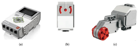
Figure 1. Components of the LEGO^® MINDSTORMS^® EV3 kit: (a) EV3 intelligent brick, (b) EV3 gyro sensor, (c) large EV3 servo motor.

2.1.2. EV3 Gyro Sensor

These sensors can be seen in Figure 1b, and are capable of detecting angular velocity up to a rate of ±440°/s. They have an accuracy of 3° on a 90° turn, and possess a 1 KHz sample rate.

2.1.3. Large EV3 Servo Motor

In Figure 1c, the large EV3 servo motor is shown. These direct current motors provide actuation to the system, and include an internal encoder to measure the angular displacement of the motor shaft. Although this motor has a gearbox, the encoder provides the angular position after the reduction of the gearbox. The motor has a maximum angular velocity of 170 rpm, a dynamic torque of 0.2 Nm, and a static torque of 0.4 Nm.

2.2. SOLIDWORKS^® Assembly of the EV3BRS

The EV3BRS is composed of a single EV3 intelligent brick, two EV3 gyro sensors, and two large EV3 servo motors. In Figure 2, the generalized coordinates of the EV3BRS are shown. As stated in [1], it is convenient to choose the generalized coordinates in such way that these be directly related with measurable signals; so, in this case, the angular displacement of the body in both planes ($q_{1x}$ y $q_{1y}$ ) and the angular position of the wheels in both planes ($q_{2x}$ and $q_{2y}$) are chosen.

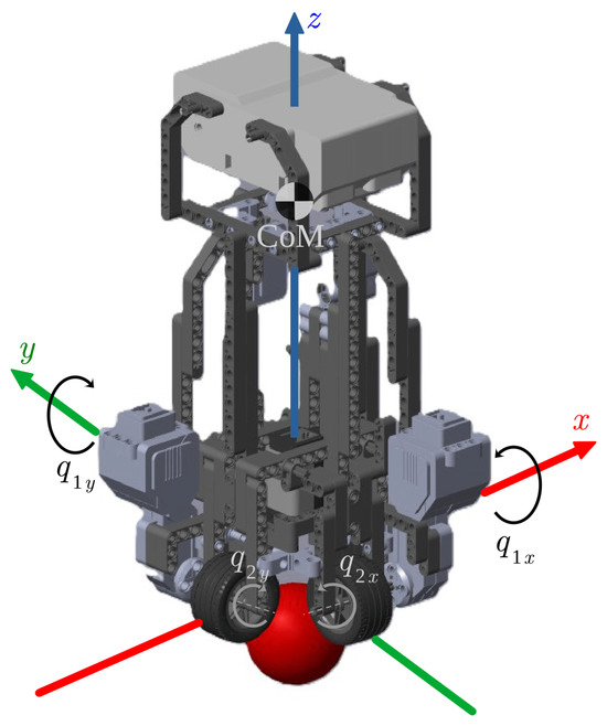
Figure 2. Generalized coordinates of the EV3BRS.

As previously stated, LEGO^® MINDSTORMS^® is a widely known brand, and many pieces are already designed and available in repositories, so the majority of LEGO^® pieces used in the assembly are obtained from the projects [14,15,16]. The only pieces designed in SOLIDWORKS^® by the authors are those shown in Figure 3.

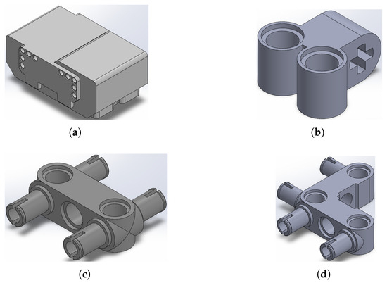
Figure 3. Pieces designed by the authors: (a) LEGO^®’s EV3 Brick, (b) LEGO^®’s piece 32291, (c) LEGO^®’s piece 48989, (d) LEGO^®’s piece 55615.

The assembly of the EV3BRS is based on the NXTBRS, proposed by [7], which is very similar to that used in [9]. One of the properties of the Simscape^™ Multibody^™ Link plugin is that the mating relationships defined in SOLIDWORKS^® are exported as joints to Simscape^™, but mates defined in subassemblies will be interpreted as rigid transforms, that is to say, rigidly attached. Since the body is considered rigid, only the mates of the wheels are defined in the assembly. Figure 4 shows the subassemblies for the body and the wheels.

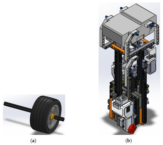
Figure 4. Subassemblies used for the overall assembly of the EV3BRS: (a) subassembly of the EV3BRS’s wheels, (b) subassembly of the EV3BRS’s body.

The finished assembly of the EV3BRS is shown in Figure 5.

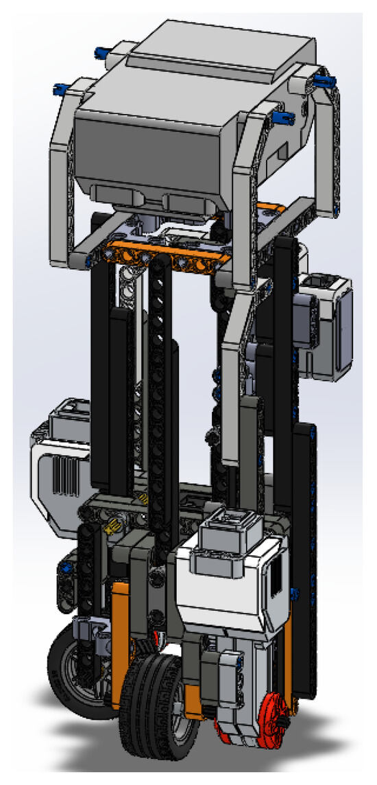
Figure 5. Entire assembly of the EV3BRS in SOLIDWORKS^®.

2.3. Simscape^™ Model of the EV3BRS

As stated previously, the assembly of the EV3BRS is exported to Simscape^™ through the Simscape^™ Multibody^™ Link plugin, giving as a result the diagram in Figure 6. It can be seen that the body of the EV3BRS is rigidly connected to the World Frame and therefore, the only thing allowed to move are the wheels. To model the entire system, the ball, the floor, and the DoF from the ball and body need to be added.

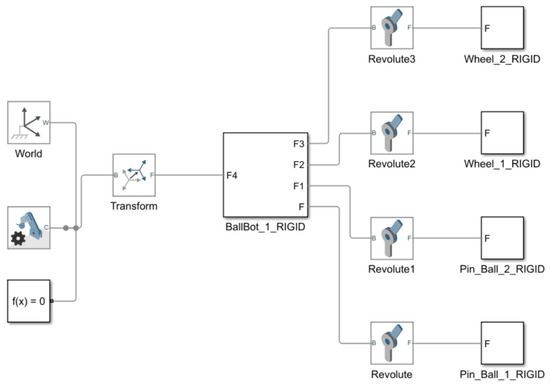
Figure 6. Unmodified EV3BRS model in Simscape^™.

In Figure 7, the whole model of the EV3BRS in Simscape^™ is shown. It can be seen that the model is divided into different areas which are described next.

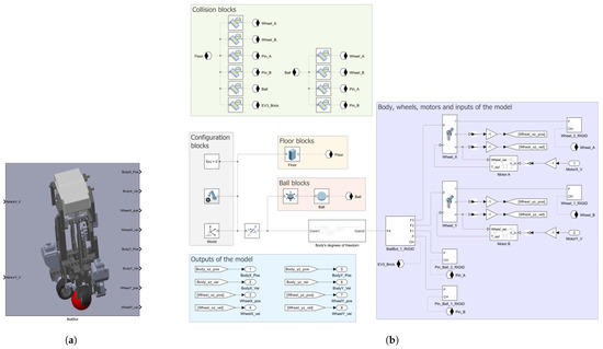
Figure 7. Comprehensive model of the EV3BRS in Simscape^™: (a) main subsystem for the EV3BRS virtual model, (b) elements of the subsystem divided into areas according to their purpose.

2.3.1. Configuration Blocks

These blocks serve as the source for parametric configuration as a starting point for the simulation. The Solver Configuration block defines the required parameters for the solver. The Mechanism Configuration block acts as the source of uniform gravity for the simulation. In our model, the gravity is defined pointing downwards along the vertical z-axis as $\left[xyz\right]=[00-9.80665][\mathrm{m}/{\mathrm{s}}^2]$. Finally, the World Frame serves as the main reference frame for the model and it is used to define all the remaining frames in the model.

2.3.2. Floor Blocks

The EV3BRS needs a surface on top of which it can move; in other words, it needs a floor. The floor is directly attached to the World Frame and consists of a Brick Solid with dimensions $\left[xyz\right]=\left[10100.01\right]\left[\mathrm{m}\right]$. The geometry of this block is exported to be used with the Collision blocks.

2.3.3. Ball Blocks

The ball is defined using the Spherical Solid block with a radius of $0.0256\left[\mathrm{m}\right]$ and, like the floor, its geometry is exported to the Collision blocks. The DoF of the ball are given through the 6-DOF Joint. It can be noticed that before the 6-DOF Joint, a Rigid Transform block is used. This latter block is used to elevate the ball $3.2\left[\mathrm{cm}\right]$ from the World Frame, in order to prevent that the ball stars “inside” the floor, that is to say, submerged inside the floor.

2.3.4. Outputs of the Model

These blocks are simply the states of the system measured from the joints of the model. The units for the outputs are given in $\left[\mathrm{rad}\right]$, for position, and $[\mathrm{rad}/\mathrm{s}]$, for the velocity.

2.3.5. Body, Wheels, Motors, and Inputs to the Model

The body and wheels are the same blocks and subsystems obtained from the Simscape^™ Multibody^™ Link plugin, but the geometry of the wheels, pins, and EV3 brick are exported to the Collision blocks. The position and velocity of the wheels are measured directly from the joints provided by the plugin.

As previously stated, the large EV3 servo motors are direct current motors with a gearbox and an encoder. Because the encoder provides the angular position of the gearbox output, the gear reduction is not model. The motor is modeled in Simscape^™ where the output shaft behavior reflects the measured encoder position. In Figure 8, the model of the motors is shown and its parameters are given in Table 1. These values are obtained from [17,18], and are also reported in [9,19]. It must be noticed that only the viscous friction is considered; the remaining parameters for the Rotational Friction are set to zero.

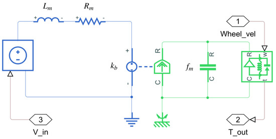
Figure 8. Motor’s model in Simscape^™.

Table 1. Motor’s parameters.

Parameter	Notation	Value	Units
Armature inductance	$L_m$	$4.94$	mH
Armature resistance	$R_m$	$6.69$	$\mathrm{\Omega }$
Body–Motor friction coefficient	$f_m$	$0.0022$	$\mathrm{N}·\mathrm{m}·\mathrm{s}/\mathrm{rad}$
Back EMF constant	$k_b$	$0.468$	$\mathrm{V}·\mathrm{s}/\mathrm{rad}$
Torque constant	$k_t$	$0.317$	$\mathrm{N}·\mathrm{m}/\mathrm{A}$
Moment of inertia	$I_M$	$1\times {10}^{-5}$	$\mathrm{Kg}·{\mathrm{m}}^2$

The inputs of the model are the motor input voltages. These are expected to be Simulink^® 10.7 (R2023a) (Mathworks, Natick, MA, USA) input signals, so they must be converted into physical signals, namely Simscape^™ signals, before they can interact with the model of the motors. This last task is performed through the Simulink-PS Converter block.

2.3.6. Collision Blocks

To model the collision, the Spatial Contact Force block is used. This block allows one to model the collision force between two bodies as well as the friction between them. The blocks used for the collisions with the floor are left with the default parameters. Instead, about the collisions with the ball, only the coefficients of friction are changed; specifically, the Coefficient of Static Friction is set to $0.70005$ while the Coefficient of Dynamic Friction is set to $0.7$. It must be noticed that these coefficients were obtained heuristically.

2.3.7. Body’s DoF

This subsystem contains all the blocks that define the DoF for the body and these are shown in Figure 9. Unlike the ball, the body obtains its DoF from several blocks; this is performed in order to have straight access to the body’s angular position and velocity. The measurements of these states are given in physical signals, and similarly to the inputs of the model, these must be converted to Simulink^® output signals, which can be accomplished through the PS-Simulink Converter block.

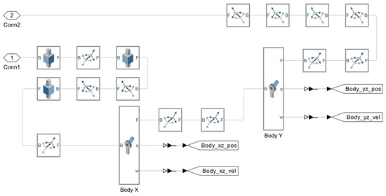
Figure 9. Blocks of the body’s DoF subsystem.

3. Mathematical Model and Control Design

3.1. Mathematical Model

The mathematical model of the EV3BRS discribed below was proposed by [7] and it was also used in [9,10,19]. This model considers the assumptions proposed in [2]:

• The EV3BRS is composed of two parts: a rigid body on top of a rigid ball.
• The movement of the roll and pitch planes are uncoupled and the equations of motion between the two planes are identical (See Figure 10b).
  

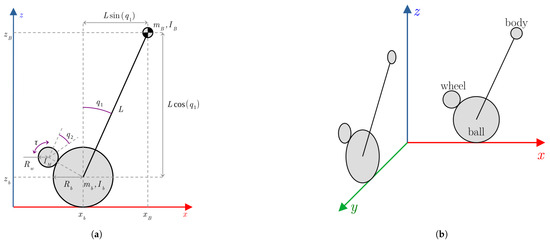  Figure 10. Simplified model of the EV3BRS: (a) simplified model for the $x-z$ plane, (b) diagram that shows the $x-z$ and $y-z$ planes as identical and uncoupled.
• The control torques are applied between the body and the ball using the wheels.
• Only viscous friction is considered.
• There is no slip between the ball and the wheels.

3.1.1. Dynamic Model

The simplified model for the $x-z$ plane is shown in Figure 10a. As stated in [1], it is convenient to choose the generalized coordinates in such way that these be directly related with measurable signals; so, in this case the angular displacement of the body ($q_1$) and wheels ($q_2$) are chosen.

The mathematical model is derived using the Euler–Lagrange method and can be expressed as follows:

$$\mathit{M}\left(\mathit{q}\right)\ddot{\mathit{q}}+\mathit{C}(\mathit{q},\dot{\mathit{q}})\ddot{\mathit{q}}+\mathit{g}\left(\mathit{q}\right)+\mathit{f}\left(\dot{\mathit{q}}\right)=\mathit{\tau },$$

(1)

where $\mathit{q}={\left[q_1{q}_2\right]}^{\top }$, $\mathit{\tau }={\left[\tau 0\right]}^{\top }$ is the control input vector, and $\tau \in \mathbb{R}$ is the input torque control. $\mathit{M}\left(\mathit{q}\right)\in {\mathbb{R}}^{2\times 2}$ is the inertia matrix, $\mathit{C}(\mathit{q},\dot{\mathit{q}})\in {\mathbb{R}}^{2\times 2}$ is the centripetal and Coriolis force matrix, $\mathit{g}\left(\mathit{q}\right)\in {\mathbb{R}}^2$ is the gravity vector, and $\mathit{f}\left(\dot{\mathit{q}}\right)\in {\mathbb{R}}^2$ is the friction vector. The elements of the matrices and vectors previously stated are the following:

$$\mathit{M}\left(\mathit{q}\right)=\left[\begin{array}{cc}{m}_{11}& m_{12}\\ m_{21}& m_{22}\end{array}\right];\mathit{C}(\mathit{q},\dot{\mathit{q}})=\left[\begin{array}{cc}{c}_{11}& 0\\ c_{21}& 0\end{array}\right];\mathit{g}\left(\mathit{q}\right)=\left[\begin{array}{c}{g}_1\\ 0\end{array}\right];\mathit{f}\left(\dot{\mathit{q}}\right)=\left[\begin{array}{c}{f}_1\\ f_2\end{array}\right],$$

where

$$\begin{array}{cccccc}\hfill m_{11}& =I_B+I_M+I_b+m_B{L}^2+m_B{R}_b^2+m_b{R}_b^2+2m_{B}L{R}_{b}cos\left(q_1\right),\hfill & \hfill c_{11}& =-m_{B}L{R}_{b}sin\left(q_1\right){\dot{q}}_1,\hfill & \hfill f_1& =f_{B_g}{\dot{q}}_1,\hfill \\ \hfill m_{12}& =I_M+I_{b}N+m_{B}N{R}_b^2+m_{b}N{R}_b^2+m_{B}LN{R}_{b}cos\left(q_1\right),\hfill & \hfill c_{21}& =-m_{B}LN{R}_{b}sin\left(q_1\right){\dot{q}}_1,\hfill & \hfill f_2& =f_{B_b}{\dot{q}}_2,\hfill \\ \hfill m_{21}& =m_{12},\hfill & \hfill g_1& =-gL{m}_{B}sin\left(q_1\right),\hfill & \hfill & \\ \hfill m_{22}& =I_M+I_b{N}^2+m_b{R}_b^2{N}^2+m_B{R}_b^2{N}^2.\hfill & \hfill & & \hfill & \end{array}$$

The notation and values from these last parameters are given in Table 2. The mass of both body and ball as well as the radius of the ball and wheels were measured experimentally. The distance to the center of mass is taken from [7]. The moments of inertia of the body and ball are extracted from [6,7]. The moments of inertia were also used in [9,19].

Table 2. Parameters of the EV3BRS.

Parameter	Notation	Value	Units
Body mass	$m_B$	$0.75$	Kg
Ball mass	$m_b$	$0.014$	Kg
Ball radius	$R_b$	$0.0256$	m
Wheel radius	$R_w$	$0.02141$	m
Distance to the center of mass	L	$0.1956$	m
Body moment of inertia	$I_B$	${\displaystyle \frac{m_B{L}^2}{3}}$	$\mathrm{Kg}·{\mathrm{m}}^2$
Ball moment of inertia	$I_b$	${\displaystyle \frac{2m_B{R}_b^2}{3}}$	$\mathrm{Kg}·{\mathrm{m}}^2$
Gear ratio	N	$-{\displaystyle \frac{R_w}{R_b}}$	-
Body–Ball friction coefficient	$f_{B_b}$	$0.0022$	$\mathrm{N}·\mathrm{m}·\mathrm{s}/\mathrm{rad}$
Body–Floor friction coefficient	$f_{B_g}$	0	$\mathrm{N}·\mathrm{m}·\mathrm{s}/\mathrm{rad}$
Gravity acceleration	g	$9.81$	$\mathrm{m}/{\mathrm{s}}^2$

3.1.2. Dynamic of the Motor

The model proposed by [7] takes into account a simplified model for the motors (see Figure 11); the inductance and friction are considered negligible (i.e., $L_a\approx 0$ and $f_m\approx 0$), so the control input vector is given by

$$\mathit{\tau }=\left[\begin{array}{c}0\\ \tau \end{array}\right]=\left[\begin{array}{c}0\\ {\displaystyle \frac{k_t\left(v-k_b{\dot{q}}_2\right)}{R_m}}\end{array}\right].$$

(2)

where v is the input voltage for the motor.

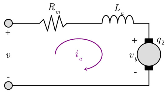
Figure 11. Simplified model for the motor.

3.1.3. State Space Representation

Defining the state vector $\mathit{x}={\left[x_1{x}_2{x}_3{x}_4\right]}^{\top }={\left[q_1{q}_2{\dot{q}}_1{\dot{q}}_2\right]}^{\top }$, the control input $u=v$, and using (2), the model (1) can be rewritten as

$$\dot{\mathit{x}}=\left[\begin{array}{cccc}0& 0& 1& 0\\ 0& 0& 0& 1\\ 0& 0& \mathrm{\Delta }\left(m_{12}{c}_{12}-m_{22}{c}_{11}-m_{22}{f}_{B_g}\right)& \mathrm{\Delta }{m}_{12}\left(f_{B_b}+{\displaystyle \frac{k_t{k}_b}{R_m}}\right)\\ 0& 0& \mathrm{\Delta }\left(m_{21}{c}_{11}-m_{11}{c}_{12}+m_{21}{f}_{B_g}\right)& -\mathrm{\Delta }{m}_{11}\left(f_{B_b}+{\displaystyle \frac{k_t{k}_b}{R_m}}\right)\end{array}\right]\mathit{x}+\left[\begin{array}{c}0\\ 0\\ -\mathrm{\Delta }{m}_{12}{\displaystyle \frac{k_t}{R_m}}\\ \mathrm{\Delta }{m}_{11}{\displaystyle \frac{k_t}{R_m}}\end{array}\right]v+\left[\begin{array}{c}0\\ 0\\ -\mathrm{\Delta }{m}_{22}{g}_1\\ \mathrm{\Delta }{m}_{21}{g}_1\end{array}\right],$$

(3)

where

$$\mathrm{\Delta }={\displaystyle \frac{1}{det\left[M\left(\mathit{q}\right)\right]}}={\displaystyle \frac{1}{m_{11}{m}_{22}-m_{12}{m}_{21}}}.$$

(4)

3.2. Linear Quadratic Regulator (LQR)

According to [20], the LQR is an optimal control that aims to minimize the cost function

$$\mathit{J}={\int }_0^{\infty }\left\{{\mathit{x}}^{\top }\mathit{Q}\mathit{x}+{\mathit{u}}^{\top }\mathit{R}\mathit{u}\right\}d\tau ,$$

(5)

where $Q=Q^{\top }\ge 0$ and $R=R^{\top }>0$. To design an LQR, the algebraic Riccati equation must be solved:

$$\mathit{P}\mathit{A}+{\mathit{A}}^{\top }\mathit{P}-\mathit{P}\mathit{B}{\mathit{R}}^{-1}{\mathit{B}}^{\top }\mathit{P}+\mathit{Q}=\mathbf{0},$$

(6)

resulting in a control feedback gain vector

$${\mathit{K}}_{\mathit{lqr}}={\mathit{R}}^{-1}{\mathit{B}}^{\top }\mathit{P}$$

(7)

with the state feedback control law

$$\mathit{u}={\mathit{K}}_{\mathit{lqr}}\mathit{x}.$$

(8)

3.2.1. Linearization of the EV3BRS’s Model Around $\left|x_1\right|=0$

Since the LQR is a linear controller, to obtain the feedback gain vector, the nonlinear model (3) is linearized around $\left|x_1\right|=0$. Using small-angle linearization for $\left|x_1\right|=0$ ($cos\left(x_1\right)\approx 1$ and $sin\left(x_1\right)\approx x_1$), the linear model takes the form

$$\dot{\mathit{x}}={\mathit{A}}_1\mathit{x}+{\mathit{B}}_{1}v=\left[\begin{array}{cccc}0& 0& 1& 0\\ 0& 0& 0& 1\\ -{\mathrm{\Delta }}_{1}W{m}_{22}& 0& 0& {\mathrm{\Delta }}_1{m}_{12}^{*}\left(f_{B_b}+{\displaystyle \frac{k_t{k}_b}{R_m}}\right)\\ {\mathrm{\Delta }}_{1}W{m}_{12}^{*}& 0& 0& -{\mathrm{\Delta }}_1{m}_{11}^{*}\left(f_{B_b}+{\displaystyle \frac{k_t{k}_b}{R_m}}\right)\end{array}\right]\mathit{x}+\left[\begin{array}{c}0\\ 0\\ -{\mathrm{\Delta }}_1{m}_{12}^{*}{\displaystyle \frac{k_t}{R_m}}\\ {\mathrm{\Delta }}_1{m}_{11}^{*}{\displaystyle \frac{k_t}{R_m}}\end{array}\right]v,$$

(9)

where

$$\begin{array}{cccc}\hfill m_{11}^{*}& =I_B+I_M+I_b+m_B{L}^2+m_B{R}_b^2+m_b{R}_b^2+2m_{B}L{R}_b,\hfill & \hfill W& =-gL{m}_B,\hfill \\ \hfill m_{12}^{*}& =I_M+I_{b}N+m_{B}N{R}_b^2+m_{b}N{R}_b^2+m_{B}LN{R}_b,\hfill & \hfill {\mathrm{\Delta }}_1& ={\displaystyle \frac{1}{m_{11}^{*}{m}_{22}-{\left(m_{12}^{*}\right)}^2}}.\hfill \end{array}$$

Given the parametric values from Table 1 and Table 2, the model (9) takes the form

$$\dot{\mathit{x}}=\left[\begin{array}{cccc}0& 0& 1& 0\\ 0& 0& 0& 1\\ 123.938359& 0& 0& -20.401434\\ 1204.484501& 0& 0& -264.663167\end{array}\right]\mathit{x}+\left[\begin{array}{c}0\\ 0\\ 39.658405\\ 514.479463\end{array}\right]v.$$

(10)

3.2.2. LQR for the EV3BRS

Solving the algebraic Riccati equation is a complex part of the LQR design; to simplify this process, the MATLAB^® 9.14 (R2023a) command lqr is used. Defining

$$\mathit{Q}=\left[\begin{array}{cccc}1500& 0& 0& 0\\ 0& 10& 0& 0\\ 0& 0& 10& 0\\ 0& 0& 0& 1\end{array}\right],R=1,$$

(11)

using (10), the feedback gain vector obtain from the command lqr is

$${\mathit{K}}_{\mathit{lqr}}=\left[\begin{array}{cccc}255.16& -3.1623& 44.915& -2.7984\end{array}\right].$$

(12)

3.3. Takagi–Sugeno Fuzzy Model (TSFM)

A TSFM describes a system as a set of fuzzy if–then rules [21,22]. Using the local approximation in fuzzy partition spaces approach, each rule is linked to a local linear system obtained from the linearization around selected interest points. Then, the overall TSFM is derived by fuzzy blending of the local linear systems. The i-th rule of a TSFM takes the form

$$\begin{array}{c}\mathbf{Model} \mathit{i}\mathbf{-th} \mathbf{rule}:\hfill \\ \mathbf{IF}{z}_1\mathrm{is}{M}_{i1}\mathrm{and}\dots z_p\mathrm{is}{M}_{ip},\hfill \\ \mathbf{THEN}\left\{\begin{array}{c}\dot{\mathit{x}}={\mathit{A}}_i\mathit{x}+{\mathit{B}}_i\mathit{u},\hfill \\ \mathit{y}={\mathit{C}}_i\mathit{x}\hfill \end{array}\right.\hfill \end{array},i=1,2,\dots ,r;$$

(13)

where $M_{ij}$ are fuzzy sets, $\mathit{x}\in {\mathbb{R}}^n$ is the state vector, $\mathit{y}\in {\mathbb{R}}^q$ is the output vector, $\mathit{u}\in {\mathbb{R}}^m$ is the input vector, ${\mathit{A}}_i\in {\mathbb{R}}^{n\times n}$ is the state matrix, ${\mathit{B}}_i\in {\mathbb{R}}^{n\times m}$ is the input matrix, ${\mathit{C}}_i\in {\mathbb{R}}^{q\times n}$ is the output matrix, $z_1,\dots ,z_p$ are known premise variables, and r is the number of rules. Defining $\mathit{z}={\left[z_1\dots z_p\right]}^{\top }\in {\mathbb{R}}^p$, the final outputs of the TSFM, given a pair of $\left(\mathit{x},\mathit{u}\right)$, are inferred as follows:

$$\begin{array}{cc}\hfill \dot{\mathit{x}}& =\sum _{i=1}^r{h}_i\left(\mathit{z}\right)\left\{{\mathit{A}}_i\mathit{x}+{\mathit{B}}_i\mathit{u}\right\},\hfill \\ \hfill \mathit{y}& =\sum _{i=1}^r{h}_i\left(\mathit{z}\right){\mathit{C}}_i\mathit{x},\hfill \end{array}$$

(14)

where $w_i\left(\mathit{z}\right)={\prod }_{j=1}^p{M}_{ij}\left(z_j\right)$, with $M_{ij}(·)$ as the grade of membership of $z_j$ in $M_{ij}$, and

$$h_i\left(\mathit{z}\right)={\displaystyle \frac{w_i\left(\mathit{z}\right)}{{\sum }_{i=1}^r{w}_i\left(\mathit{z}\right)}}$$

(15)

the normalized weight of the i-th rule.

3.3.1. Linearization of the EV3BRS’s Model Around $\left|x_1\right|={\displaystyle \frac{\pi }{12}}$

In order to derive the TSFM of the EV3BRS, the nonlinear model (3) is linearized around $\left|x_1\right|=0$ and $\left|x_1\right|={\displaystyle \frac{\pi }{12}}$. The system has already been linearized around $\left|x_1\right|=0$, as shown in (10). Now, for $\left|x_1\right|={\displaystyle \frac{\pi }{12}}$ the following is considered:

$$cos\left(x_1\right)\approx cos\left({\displaystyle \frac{\pi }{12}}\right),sin\left(x_1\right)\approx {\displaystyle \frac{sin\left(\frac{\pi }{12}\right)}{\frac{\pi }{12}}}{x}_1={\xi }_1{x}_1.$$

(16)

Thus, the local linear model takes the form

$$\dot{\mathit{x}}={\mathit{A}}_2\mathit{x}+{\mathit{B}}_{2}v=\left[\begin{array}{cccc}0& 0& 1& 0\\ 0& 0& 0& 1\\ -{\mathrm{\Delta }}_{2}W{\xi }_1{m}_{22}& 0& 0& {\mathrm{\Delta }}_2{m}_{12}^{**}\left(f_{B_b}+{\displaystyle \frac{k_t{k}_b}{R_m}}\right)\\ {\mathrm{\Delta }}_{2}W{\xi }_1{m}_{12}^{**}& 0& 0& -{\mathrm{\Delta }}_2{m}_{11}^{**}\left(f_{B_b}+{\displaystyle \frac{k_t{k}_b}{R_m}}\right)\end{array}\right]\mathit{x}+\left[\begin{array}{c}0\\ 0\\ -{\mathrm{\Delta }}_2{m}_{12}^{**}{\displaystyle \frac{k_t}{R_m}}\\ {\mathrm{\Delta }}_2{m}_{11}^{**}{\displaystyle \frac{k_t}{R_m}}\end{array}\right]v,$$

(17)

where

$$\begin{array}{cc}\hfill m_{11}^{**}& =I_B+I_M+I_b+m_B{L}^2+m_B{R}_b^2+m_b{R}_b^2+2m_{B}L{R}_{b}cos\left({\displaystyle \frac{\pi }{12}}\right),\hfill \\ \hfill m_{12}^{**}& =I_M+I_{b}N+m_{B}N{R}_b^2+m_{b}N{R}_b^2+m_{B}LN{R}_{b}cos\left({\displaystyle \frac{\pi }{12}}\right).\hfill \end{array}$$

Again, using the parametric values from Table 1 and Table 2, Equation (17) takes the form

$$\dot{\mathit{x}}=\left[\begin{array}{cccc}0& 0& 1& 0\\ 0& 0& 0& 1\\ 106.078267& 0& 0& -17.130803\\ 999.8752898& 0& 0& -227.865513\end{array}\right]\mathit{x}+\left[\begin{array}{c}0\\ 0\\ 33.300615\\ 442.948402\end{array}\right]v.$$

(18)

3.3.2. EV3BRS’s TSFM

Since the model (3) is only linearized around two points, the TSFM is only comprised of two rules. Defining ${\mathit{C}}_1={\mathit{C}}_2=\left[1000\right]$, the rules of the TSFM are the following:

$$\begin{array}{c}\mathbf{Model}\mathbf{1}\mathbf{st}\mathbf{rule}:\hfill \\ \mathbf{IF}\left|x_1\right|\mathrm{is}\mathrm{about}0,\hfill \\ \mathbf{THEN}\left\{\begin{array}{cc}\hfill & \dot{\mathit{x}}={\mathit{A}}_1\mathit{x}+{\mathit{B}}_{1}v,\hfill \\ \hfill & \mathit{y}={\mathit{C}}_1\mathit{x}\hfill \end{array}\right.\hfill \end{array}$$

(19)

$$\begin{array}{c}\mathbf{Model}\mathbf{2}\mathbf{nd}\mathbf{rule}:\hfill \\ \mathbf{IF}\left|x_1\right|\mathrm{is}\mathrm{about}{\displaystyle \frac{\pi }{12}},\hfill \\ \mathbf{THEN}\left\{\begin{array}{cc}\hfill & \dot{\mathit{x}}={\mathit{A}}_2\mathit{x}+{\mathit{B}}_{2}v,\hfill \\ \hfill & \mathit{y}={\mathit{C}}_2\mathit{x}\hfill \end{array}\right.\hfill \end{array}$$

(20)

These rules can be expressed in the form of (14) using the membership functions shown in Figure 12. So, the TSFM of the EV3BRS takes the form

$$\begin{array}{cc}\hfill \dot{\mathit{x}}& =\sum _{i=1}^2{h}_i\left(\left|x_1\right|\right)\left\{{\mathit{A}}_i\mathit{x}+{\mathit{B}}_{i}v\right\},\hfill \\ \hfill \mathit{y}& =\sum _{i=1}^2{h}_i\left(\left|x_1\right|\right){\mathit{C}}_i\mathit{x},\hfill \end{array}$$

(21)

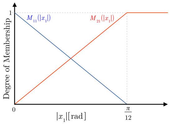
Figure 12. Membership functions of the EV3BRS’s TSFM.

3.4. Takagi–Sugeno Fuzzy Control (TSFC)

To design a TSFC, the Parallel Distributed Compensation (PDC) technique is used [22]. A feedback control law $\mathit{u}=-{\mathit{K}}_i\mathit{x}$, where ${\mathit{K}}_i\in {\mathbb{R}}^{m\times n}$ is the i-th feedback gain vector, can be applied to stabilize each local linear system of the TSFM. Thus, the PDC comprises of the same amount of rules as the TSFM and also shares its fuzzy sets. Then, the PDC can be described as a set of rules given in the following form:

$$\begin{array}{c}\mathbf{Control}\mathbf{i}\mathbf{-th}\mathbf{rule}:\hfill \\ \mathbf{IF}{z}_1\mathrm{is}{M}_{i1}\mathrm{and}\dots z_p\mathrm{is}{M}_{ip},\hfill \\ \mathbf{THEN}\mathit{u}=-{\mathit{K}}_i\mathit{x}\hfill \end{array}\hspace{1em},\hspace{1em}i = 1, 2,\dots , r;$$

(22)

Using the same membership functions as in the TSFM, the overall PDC can be described in the form

$$\mathit{u}=-\sum _{i=1}^r{h}_i\left(z\right){\mathit{K}}_i\mathit{x}.$$

(23)

3.4.1. Stable TSFC

To determine the feedback gain vector $K_i$ that ensures global stability, the following theorem must be satisfied.

Theorem 1

([23]). The TSFM (14) with the PDC control law (23) is globally asymptotically stable if there exist matrices $\mathit{X}={\mathit{X}}^{\top }>0$, and ${\mathit{M}}_i,i=1,2,\dots ,r$, such that

$${\mathbf{\Gamma }}_{ij}=\mathit{X}{\mathit{A}}_i^{\top }+{\mathit{A}}_i\mathit{X}-{\mathit{M}}_j^{\top }{\mathit{B}}_i^{\top }-{\mathit{B}}_i{\mathit{M}}_j,$$

satisfies the following conditions:

$$\begin{array}{c}\hfill {\mathbf{\Gamma }}_{ii}<0,\\ \hfill {\mathbf{\Gamma }}_{ij}+{\mathbf{\Gamma }}_{ji}<0,\end{array}$$

(24)

for $i=1,2,\dots ,r$ and $j=i+1,i+2,\dots ,r$. If these conditions are satisfied, the PDC gains are ${\mathit{K}}_i={\mathit{M}}_i{\mathit{X}}^{-1},i=1,2,\dots ,r$.

Proof. 

See [23]. □

Applying Theorem 1 to the TSFM (21) of the EV3BRS, the following Linear Matrix Inequalities (LMIs) must be solved:

$$\begin{array}{cc}\hfill {\mathbf{\Gamma }}_{11}& <0\hfill \end{array}$$

(25)

$$\begin{array}{cc}\hfill {\mathbf{\Gamma }}_{22}& <0\hfill \end{array}$$

(26)

$$\begin{array}{cc}\hfill {\mathbf{\Gamma }}_{12}+{\mathbf{\Gamma }}_{21}& <0\hfill \end{array}$$

(27)

where

$$\begin{array}{cc}\hfill {\mathbf{\Gamma }}_{11}& =\mathit{X}{\mathit{A}}_1^{\top }+{\mathit{A}}_1\mathit{X}-{\mathit{M}}_1^{\top }{\mathit{B}}_1^{\top }-{\mathit{B}}_1{\mathit{M}}_1\hfill \end{array}$$

(28)

$$\begin{array}{cc}\hfill {\mathbf{\Gamma }}_{22}& =\mathit{X}{\mathit{A}}_2^{\top }+{\mathit{A}}_2\mathit{X}-{\mathit{M}}_2^{\top }{\mathit{B}}_2^{\top }-{\mathit{B}}_2{\mathit{M}}_2\hfill \end{array}$$

(29)

$$\begin{array}{cc}\hfill {\mathbf{\Gamma }}_{12}& =\mathit{X}{\mathit{A}}_1^{\top }+{\mathit{A}}_1\mathit{X}-{\mathit{M}}_2^{\top }{\mathit{B}}_1^{\top }-{\mathit{B}}_1{\mathit{M}}_2\hfill \end{array}$$

(30)

$$\begin{array}{cc}\hfill {\mathbf{\Gamma }}_{21}& =\mathit{X}{\mathit{A}}_2^{\top }+{\mathit{A}}_2\mathit{X}-{\mathit{M}}_1^{\top }{\mathit{B}}_2^{\top }-{\mathit{B}}_2{\mathit{M}}_1\hfill \end{array}$$

(31)

Using the YALMIP toolbox and choosing the SeDuMi 1.3.7 solver with the adaptative self-differentiation method to solve the LMIs, the following matrices are obtained:

$$\begin{array}{cc}\hfill \mathit{X}& =\left[\begin{array}{cccc}0.014396& 0.00032416& -0.080298& -0.0029134\\ 0.00032416& 25.382& -0.0015091& -0.42286\\ -0.080298& -0.0015091& 0.44804& 0.019218\\ -0.0029134& -0.42286& 0.019218& 0.076509\end{array}\right],\hfill \\ \hfill {\mathit{M}}_1& =\left[\begin{array}{cccc}0.035395& 0.21844& -0.19866& -0.04262\end{array}\right],\hfill \\ \hfill {\mathit{M}}_2& =\left[\begin{array}{cccc}0.03426& 0.21847& -0.1923& -0.042139\end{array}\right].\hfill \end{array}$$

Thus, the feedback gain vectors are

$$\begin{array}{cc}\hfill {\mathit{K}}_1& =\left[\begin{array}{cccc}56.01& -0.0061596& 9.6323& -0.87776\end{array}\right],\hfill \end{array}$$

(32)

$$\begin{array}{cc}\hfill {\mathit{K}}_2& =\left[\begin{array}{cccc}61.681& -0.0068506& 10.665& -0.91864\end{array}\right].\hfill \end{array}$$

(33)

Therefore, using the membership functions from Figure 12, the PDC control law can be expressed in the form

$$v=-\sum _{i=1}^2{h}_i\left(\left|x_1\right|\right)K_i\mathit{x}.$$

(34)

3.4.2. TSFC with $H_{\infty }$ Attenuation

Performance criteria can be added to the control using extra LMIs [22,23]. Consider the TSFM (14) with external disturbance $\mathit{d}\in {\mathbb{R}}^l$, i.e.,

$$\begin{array}{cc}\hfill \dot{\mathit{x}}& =\sum _{i=1}^r{h}_i\left(\mathit{z}\right)\left\{A_i\mathit{x}+B_i\mathit{u}+E_i\mathit{d}\right\},\hfill \\ \hfill \mathit{y}& =\sum _{i=1}^r{h}_i\left(\mathit{z}\right)C_i\mathit{x}.\hfill \end{array}$$

(35)

Disturbance rejection can be achieved by minimizing $\gamma$ subject to

$$\underset{\mathit{d}\ne 0}{sup}{\displaystyle \frac{∥\mathit{y}∥}{∥\mathit{d}∥}}\le \gamma .$$

To add disturbance rejection to the PDC control law, the following theorem must be satisfied (it should be noted that ${\mathit{I}}_a\in {\mathbb{R}}^{a\times a}$ denotes an identity matrix)

Theorem 2

([23]). The TSFM (35) with PDC control law (23) is globally asymptotically stable and the disturbance $\mathit{d}$ is attenuated by at least γ, if there exist matrices $X>0$, and $M_i,i=1,2,\dots ,r$, such that

$${\mathbf{\Gamma }}_{ij}=\left[\begin{array}{ccc}\mathit{X}{\mathit{A}}_i^{\top }+{\mathit{A}}_i\mathit{X}-{\mathit{M}}_j^{\top }{\mathit{B}}_i^{\top }-{\mathit{B}}_i{\mathit{M}}_j& {\mathit{E}}_i& \mathit{X}{\mathit{C}}_i^{\top }\\ {\mathit{E}}_i^{\top }& -\gamma {\mathit{I}}_l& {\mathbf{0}}_{l\times q}\\ {\mathit{C}}_{i}X& {\mathbf{0}}_{q\times l}& -{\mathit{I}}_q\end{array}\right]$$

satisfies the conditions (24). If these conditions are satisfied, the PDC gains are ${\mathit{K}}_i={\mathit{M}}_i{\mathit{X}}^{-1},i=1,2,\dots ,r$.

Proof. 

See [23]. □

Considering the following input voltage disturbance:

$$d_1=\left\{\begin{array}{cc}0\hfill & t<5\hfill \\ -0.5+1.5sin\left(2t\right)+0.05t\hfill & 5\le t\le 15\hfill \\ 0\hfill & t>15\hfill \end{array}\right.\left[V\right],$$

(36)

the model (3) can be modified to include this disturbance as an input of the system. Thus, the EV3BRS’s model with input anomalies is then given as

$$\dot{\mathit{x}}=\left[\begin{array}{cccc}0& 0& 1& 0\\ 0& 0& 0& 1\\ 0& 0& \mathrm{\Delta }\left(m_{12}{c}_{12}-m_{22}{c}_{11}-m_{22}{f}_{B_g}\right)& \mathrm{\Delta }{m}_{12}\left(f_{B_b}+{\displaystyle \frac{k_t{k}_b}{R_m}}\right)\\ 0& 0& \mathrm{\Delta }\left(m_{21}{c}_{11}-m_{11}{c}_{12}+m_{21}{f}_{B_g}\right)& -\mathrm{\Delta }{m}_{11}\left(f_{B_b}+{\displaystyle \frac{k_t{k}_b}{R_m}}\right)\end{array}\right]\mathit{x}+\left[\begin{array}{c}0\\ 0\\ -\mathrm{\Delta }{m}_{12}{\displaystyle \frac{k_t}{R_m}}\\ \mathrm{\Delta }{m}_{11}{\displaystyle \frac{k_t}{R_m}}\end{array}\right](v+d)+\left[\begin{array}{c}0\\ 0\\ -\mathrm{\Delta }{m}_{22}{g}_1\\ \mathrm{\Delta }{m}_{21}{g}_1\end{array}\right].$$

(37)

To form the TSFM of the EV3 with the anomaly added, the model (37) must be linearized around $\left|x_1\right|=0$ and $\left|x_1\right|={\displaystyle \frac{\pi }{12}}$. Linearizing around $\left|x_1\right|=0$

$$\dot{\mathit{x}}={\mathit{A}}_1\mathit{x}+{\mathit{B}}_{1}v+{\mathit{E}}_{1}d=\left[\begin{array}{cccc}0& 0& 1& 0\\ 0& 0& 0& 1\\ -{\mathrm{\Delta }}_{1}W{m}_{22}& 0& 0& {\mathrm{\Delta }}_1{m}_{12}^{*}\left(f_{B_b}+{\displaystyle \frac{k_t{k}_b}{R_m}}\right)\\ {\mathrm{\Delta }}_{1}W{m}_{12}^{*}& 0& 0& -{\mathrm{\Delta }}_1{m}_{11}^{*}\left(f_{B_b}+{\displaystyle \frac{k_t{k}_b}{R_m}}\right)\end{array}\right]\mathit{x}+\left[\begin{array}{c}0\\ 0\\ -{\mathrm{\Delta }}_1{m}_{12}^{*}{\displaystyle \frac{k_t}{R_m}}\\ {\mathrm{\Delta }}_1{m}_{11}^{*}{\displaystyle \frac{k_t}{R_m}}\end{array}\right]v+\left[\begin{array}{c}0\\ 0\\ -{\mathrm{\Delta }}_1{m}_{12}^{*}{\displaystyle \frac{k_t}{R_m}}\\ {\mathrm{\Delta }}_1{m}_{11}^{*}{\displaystyle \frac{k_t}{R_m}}\end{array}\right]d,$$

(38)

Then, linearizing around $\left|x_1\right|={\displaystyle \frac{\pi }{12}}$

$$\dot{\mathit{x}}={\mathit{A}}_2\mathit{x}+{\mathit{B}}_{2}v+{\mathit{E}}_{2}d=\left[\begin{array}{cccc}0& 0& 1& 0\\ 0& 0& 0& 1\\ -{\mathrm{\Delta }}_{2}W{\xi }_1{m}_{22}& 0& 0& {\mathrm{\Delta }}_2{m}_{12}^{**}\left(f_{B_b}+{\displaystyle \frac{k_t{k}_b}{R_m}}\right)\\ {\mathrm{\Delta }}_{2}W{\xi }_1{m}_{12}^{**}& 0& 0& -{\mathrm{\Delta }}_2{m}_{11}^{**}\left(f_{B_b}+{\displaystyle \frac{k_t{k}_b}{R_m}}\right)\end{array}\right]\mathit{x}+\left[\begin{array}{c}0\\ 0\\ -{\mathrm{\Delta }}_2{m}_{12}^{**}{\displaystyle \frac{k_t}{R_m}}\\ {\mathrm{\Delta }}_2{m}_{11}^{**}{\displaystyle \frac{k_t}{R_m}}\end{array}\right]v+\left[\begin{array}{c}0\\ 0\\ -{\mathrm{\Delta }}_2{m}_{12}^{**}{\displaystyle \frac{k_t}{R_m}}\\ {\mathrm{\Delta }}_2{m}_{11}^{**}{\displaystyle \frac{k_t}{R_m}}\end{array}\right]d.$$

(39)

Using the membership functions depicted in Figure 12, (37) can be represented in a form similar to (35):

$$\begin{array}{cc}\hfill \dot{\mathit{x}}& =\sum _{i=1}^2{h}_i\left(\mathit{z}\right)\left\{{\mathit{A}}_i\mathit{x}+{\mathit{B}}_{i}v+{\mathit{E}}_{i}d\right\},\hfill \\ \hfill \mathit{y}& =\sum _{i=1}^2{h}_i\left(\mathit{z}\right){\mathit{C}}_i\mathit{x},\hfill \end{array}$$

(40)

To satisfy Theorem 2 the LMIs (25), (26), and (27) must be solved considering

$$\begin{array}{cc}\hfill {\mathbf{\Gamma }}_{11}& =\left[\begin{array}{ccc}\mathit{X}{\mathit{A}}_1^{\top }+{\mathit{A}}_1\mathit{X}-{\mathit{M}}_1^{\top }{\mathit{B}}_1^{\top }-{\mathit{B}}_1{\mathit{M}}_1& {\mathit{E}}_1& \mathit{X}{\mathit{C}}_1^{\top }\\ {\mathit{E}}_1^{\top }& -\gamma & 0\\ {\mathit{C}}_1\mathit{X}& 0& -1\end{array}\right]\hfill \end{array}$$

(41)

$$\begin{array}{cc}\hfill {\mathbf{\Gamma }}_{22}& =\left[\begin{array}{ccc}\mathit{X}{\mathit{A}}_2^{\top }+{\mathit{A}}_2\mathit{X}-{\mathit{M}}_2^{\top }{\mathit{B}}_2^{\top }-{\mathit{B}}_2{\mathit{M}}_2& {\mathit{E}}_2& \mathit{X}{\mathit{C}}_2^{\top }\\ {\mathit{E}}_2^{\top }& -\gamma & 0\\ {\mathit{C}}_2\mathit{X}& 0& -1\end{array}\right]\hfill \end{array}$$

(42)

$$\begin{array}{cc}\hfill {\mathbf{\Gamma }}_{12}& =\left[\begin{array}{ccc}\mathit{X}{\mathit{A}}_1^{\top }+{\mathit{A}}_1\mathit{X}-{\mathit{M}}_2^{\top }{\mathit{B}}_1^{\top }-{\mathit{B}}_1{\mathit{M}}_2& {\mathit{E}}_1& \mathit{X}{\mathit{C}}_1^{\top }\\ {\mathit{E}}_1^{\top }& -\gamma & 0\\ {\mathit{C}}_1\mathit{X}& 0& -1\end{array}\right]\hfill \end{array}$$

(43)

$$\begin{array}{cc}\hfill {\mathbf{\Gamma }}_{21}& =\left[\begin{array}{ccc}\mathit{X}{\mathit{A}}_2^{\top }+{\mathit{A}}_2\mathit{X}-{\mathit{M}}_1^{\top }{\mathit{B}}_2^{\top }-{\mathit{B}}_2{\mathit{M}}_1& {\mathit{E}}_2& \mathit{X}{\mathit{C}}_2^{\top }\\ {\mathit{E}}_2^{\top }& -\gamma & 0\\ {\mathit{C}}_2\mathit{X}& 0& -1\end{array}\right]\hfill \end{array}$$

(44)

Using the same solver and toolbox as in the nominal TSFC, the following matrices are obtained:

$$\begin{array}{cc}\hfill \mathit{X}& =\left[\begin{array}{cccc}9.7698& -0.7885& -54.368& 0.67473\\ -0.7885& 52167& 4.4033& -159.11\\ -54.368& 4.4033& 302.57& -3.5886\\ 0.67473& -159.11& -3.5886& 4.6188\end{array}\right],\hfill \\ \hfill {\mathit{M}}_1& =\left[\begin{array}{cccc}22.538& 79.74& -120.54& 63.723\end{array}\right],\hfill \\ \hfill {\mathit{M}}_2& =\left[\begin{array}{cccc}21.921& 80.165& -117.81& 55.758\end{array}\right].\hfill \end{array}$$

Thus, the PDC gains are

$$\begin{array}{cc}\hfill {\mathit{K}}_1& =\left[\begin{array}{cccc}4.4841\times {10}^5& -9.9688& 80536& -3262.3\end{array}\right],\hfill \end{array}$$

(45)

$$\begin{array}{cc}\hfill {\mathit{K}}_2& =\left[\begin{array}{cccc}3.7559\times {10}^5& -8.348& 67458& -2731.9\end{array}\right].\hfill \end{array}$$

(46)

Since the control law itself has not changed, the form (34) holds.

Additional unmodeled anomalies are introduced to assess the robustness of the controller. The first additional anomaly consists of a series of small torque pulses with an amplitude of $0.15[Nm]$ applied to the body, simulating an external disturbance. The second anomaly consists of uniform noise limited to $\pm 0.01[rad]$ that is applied to the angular displacement of the wheels, representing sensor inaccuracies. Figure 13 shows the anomalies considered in the simulation.

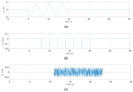
Figure 13. Anomalies considered: (a) input anomaly, (b) external anomaly, (c) noise anomaly.

4. Results

4.1. LQR on Simscape^™

As previously stated, the LQR control is simulated to serve as a benchmark for comparison against the TSFC and the TSFC with $H_{\infty }$ attenuation. To implement the LQR, the control law (8) with feedback gain vector (12) is used. The simulation is carried out using the Simulink^® model shown in Figure 14. Since the maximum voltage that the EV3 intelligent brick can provide to the motors is $\pm 8.3\left[V\right]$, a saturation block is added. To simulate the system, the solver daessc with variable step is used. The simulation is started from initial conditions ${\mathit{x}}_{\mathit{xz}}\left(0\right)={\left[0000\right]}^{\top }[deg]$ for the $x-z$ plane, and ${\mathit{x}}_{\mathit{yz}}\left(0\right)={[-5000]}^{\top }[deg]$ for the $y-z$ plane.

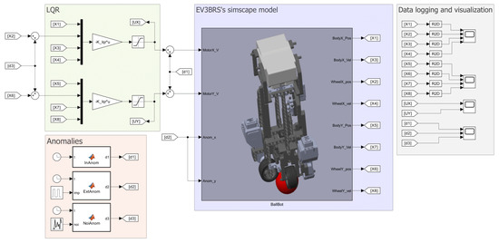
Figure 14. Implementation of the LQR to the EV3BRS’s Simscape^™ model.

The behavior of the angular position of the body is shown in Figure 15a and Figure 16a, corresponding to the $x-z$ plane and the $y-z$ plane, respectively. The angular position of the wheels is presented in Figure 15c for the $x-z$ plane and in Figure 16c for the $y-z$ plane. In all of the above figures, the beginning and end of the anomalies are denoted by vertical dashed lines: red for the input anomaly, black for the external anomaly, and magenta for the sensor noise anomaly. In Figure 17, the control signal for both planes can be seen. Since the tracking task is outside of the scope for this work, the displacement in the $x-y$ plane is not taken into consideration; thus, the TSFC successfully achieves the control objective.

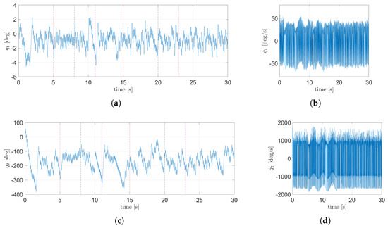
Figure 15. State dynamics corresponding to the $x-z$ plane using the LQR: (a) angular position of the body, (b) angular velocity of the body, (c) angular position of the wheel, (d) angular velocity of the wheels.

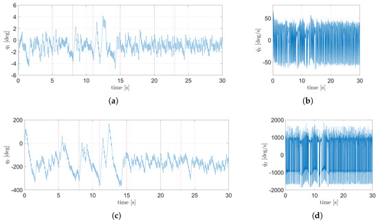
Figure 16. State dynamics corresponding to the $y-z$ plane using the LQR: (a) angular position of the body, (b) angular velocity of the body, (c) angular position of the wheel, (d) angular velocity of the wheels.

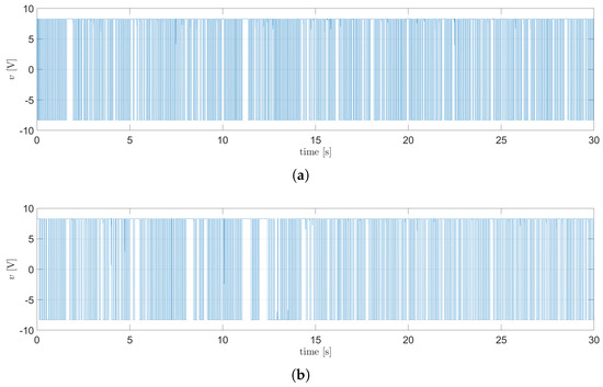
Figure 17. Control signals for the motors using the LQR: (a) signal for the $x-z$ plane, (b) signal for the $y-z$ plane.

4.2. Nominal TSFC on Simscape^™

The control law (34) with PDC gains (32) and (33) is applied to the EV3BRS Simscape^™ model as shown in Figure 18. To conduct the simulation, the same solver, saturation, and initial conditions from the LQR are used.

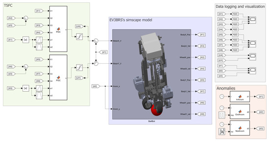
Figure 18. Implementation of the whole TSFC to the EV3BRS’s Simscape^™ model.

The evolution from the states of the system in the $x-z$ plane are shown in Figure 19, while the states corresponding to the $y-z$ plane can be seen in Figure 20. From Figure 19a and Figure 20a, it can be seen that the TSFC can maintain the body of the EV3BRS balanced over the ball (i.e., near the upright position). Figure 19c and Figure 20c show the angular displacement of the wheels. The control signal for each motor is shown in Figure 21. As mentioned above, the displacement in the $y-z$ plane is not taken into account, so the nominal TSFC fulfills the control objective. A video of the animation for this simulation is attached in the Supplementary Materials (Video S1).

Figure 19. State dynamics corresponding to the $x-z$ plane using the nominal TSFC: (a) angular position of the body, (b) angular velocity of the body, (c) angular position of the wheel, (d) angular velocity of the wheels.

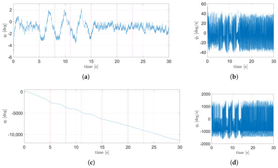
Figure 20. State dynamics corresponding to the $y-z$ plane using the nominal TSFC: (a) angular position of the body, (b) angular velocity of the body, (c) angular position of the wheel, (d) angular velocity of the wheels.

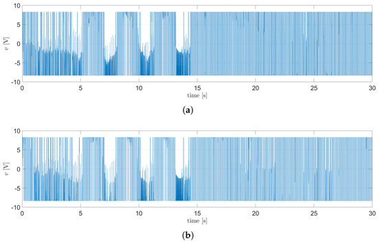
Figure 21. Control signals for the motors using the nominal TSFC: (a) signal for the $x-z$ plane, (b) signal for the $y-z$ plane.

4.3. TSFC with $H_{\infty }$ Attenuation

In order to robustify the performance of the TSFC in presence of input anomaly and the two unmodeled anomalies, the $H_{\infty }$ attenuation is invoked, where the gains (45) and (46) are consider. The same Simulink^® model, initial conditions, solver, and saturation imposed from the nominal TSFC are used. In Figure 22, the dynamic of the states corresponding to the $x-z$ plane are shown, while Figure 23 shows the dynamic of the states from the $y-z$ plane. Figure 22a and Figure 23a show the angular displacement of the body, and it can be seen that the anomalies generate smaller oscillation compared with the nominal TSFC. The angular position of the wheel can be seen in Figure 22c and Figure 23c. In Figure 22 and Figure 23 the red dotted line denotes the begging and end of the disturbance. The control signals for both planes can be seen in Figure 24. From Figure 22a and Figure 23a, it can be concluded that the control objective is achieved since the TSFC is able to maintain the body near the upright position. A video of the animation for this simulation is attached in the Supplementary Materials (Video S2).

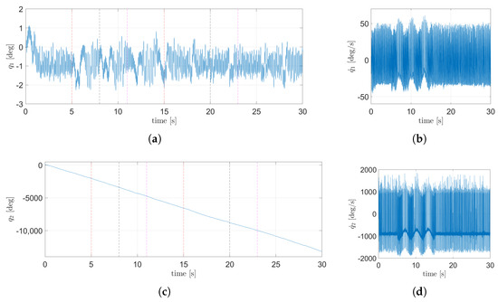
Figure 22. State dynamics corresponding to the $x-z$ plane using the TSFC with $H_{\infty }$ attenuation: (a) angular position of the body, (b) angular velocity of the body, (c) angular position of the wheel, (d) angular velocity of the wheels.

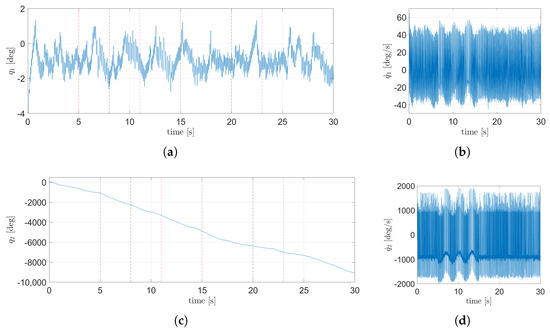
Figure 23. State dynamics corresponding to the $y-z$ plane using the TSFC with $H_{\infty }$ attenuation: (a) angular position of the body, (b) angular velocity of the body, (c) angular position of the wheel, (d) angular velocity of the wheels.

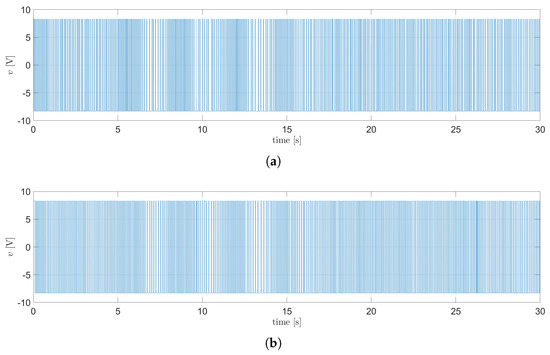
Figure 24. Control signals for the motors using the TSFC with $H_{\infty }$ attenuation: (a) signal for the $x-z$ plane, (b) signal for the $y-z$ plane.

The attenuation of the disturbance is better seen when the performance of the LQR, nominal TSFC, and the TSFC with $H_{\infty }$ attenuation is compared. Figure 25a compares the body position dynamics for plane $x-z$, while Figure 25b compares the wheel position dynamics for the same plane. Similarly, Figure 26a,b shows the corresponding dynamics for the $y-z$ plane. In Figure 25a and Figure 26a, it can be observed how the presence of anomalies induces oscillations in the angular position of the body; it must be stated that most of these oscillations are induced by the input anomaly. Figure 25b and Figure 26b shows that, under the LQR, the angular position of the wheel experiences less drift compared with the other two controllers. Table 3 compares the RMS of the input voltage and error of the angular position of the body, and the maximum error from the three controllers.

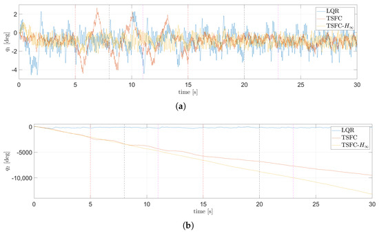
Figure 25. Comparison of the LQR, nominal TSFC, and the TSFC with $H_{\infty }$ attenuation in the $x-z$ plane: (a) angular position dynamics of the body, (b) angular position dynamics of the wheel.

Figure 26. Comparison of the LQR, nominal TSFC, and the TSFC with $H_{\infty }$ attenuation in the $y-z$ plane: (a) angular position dynamics of the body, (b) angular position dynamics of the wheel.

Table 3. Quantitative index performance.

Index *	LQR	TSFC	TSFC-${\mathit{H}}_{\mathit{\infty }}$
$\mathit{x}-\mathit{z}$  plane
$RMS\left\{e_1\right\}\left[deg\right]$	$1.430762$	$1.295060$	$\mathbf{1}.\mathbf{039813}$
$max\left\{\left|e_1\right|\right\}\left[deg\right]$	$4.571500$	$4.418068$	$\mathbf{2}.\mathbf{290599}$
$RMS\left\{v\right\}\left[V\right]$	$8.229351$	$\mathbf{7}.\mathbf{835870}$	$8.236432$
$\mathit{y}-\mathit{z}$  plane
$RMS\left\{e_1\right\}\left[deg\right]$	$1.541170$	$1.358083$	$\mathbf{1}.\mathbf{172947}$
$max\left\{\left|e_1\right|\right\}\left[deg\right]$	$5.072078$	$5.074775$	$\mathbf{5}.\mathbf{072075}$
$RMS\left\{v\right\}\left[V\right]$	$8.242265$	$\mathbf{7}.\mathbf{909134}$	$8.238710$

* $e_1=0-x_1$

5. Discussion

In summary, this work details the procedure to develop the model of the EVBRS by using the Simscape^™ environment. The use of the Simscape^™ Multibody^™ Link plugin is essential to the development of the model since it allows the design of the body of the EV3BRS to take place in SOLIDWORKS^®. Taking advantage of the popularity of LEGO^® MINDSTORMS^®, the design of most of the pieces that comprise the body is already achieved, and thus, only four pieces needed to be designed before making the assembly in SOLIDWORKS^® and exporting it to the Simscape^™ environment.

Using the EV3BRS’s Simscape^™ model allows the tuning of control gains without risking the physical platform and, although it is beyond the scope of this work, the displacement in the $x-y$ plane should be taken into consideration when preparing an area for experimental evaluation. The Simscape^™ model may be used to delimit such displacement. Importantly, this model is expected to produce simulation results that more closely match experimental behavior, and because no other EV3BRS Simscape^™ model has been reported in the literature, the model here developed can be considered a first virtual testbed that allows a more accurate control development.

All the controllers evaluated are able to fulfill the control objective, even under the presence of anomalies. It can be seen from Figure 25 and Figure 26 that the input anomaly produces the most significant effect in the angular displacement of the body, as it induces the largest oscillations. The LQR is used as a benchmark to compare the performance of the fuzzy controllers against a classical controller. Although the fuzzy controllers preform better than the LQR, the latter surpasses the fuzzy controllers in the drift of the wheels. This means that when under the LQR, the displacement on the $x-y$ plane is less than when using a fuzzy controller. The nominal TSFC has a better balance of the body when under normal conditions, but when anomalies are introduced, its performance worsens. In order to improve the behavior of the TSFC under the presence of anomalies, the $H_{\infty }$ approach is exploited. Simulation results confirm that the effect of the anomalies is reduced when the TSFC with $H_{\infty }$ attenuation is used.

6. Conclusions

From our study, the TSFC with $H_{\infty }$ attenuation has shown improvement in the performance of the EV3BRS Simscape^™ model under not only anomalies at the input, but also unmodeled anomalies. This enhanced disturbance rejection highlights the $H_{\infty }$ attenuation methodology as a way to improve control resilience.

The Simscape^™ model of the EV3BRS here developed provides a safe environment for testing and tuning different control methodology, without any risk to the physical platform. This virtual model can also be used in the development of controllers who aim to solve the trajectory tracking problem.

To the best of our knowledge, the literature does not report the development of a virtual model for a BRS developed using LEGO^® components, particularly with EV3 hardware. Since the results obtained with this virtual model are expected to be more exact, the development of this virtual model allows for a more realistic simulation of a low-cost prototype developed with EV3 components.

Although the prototype here considered is intended primarily for research purposes, the maneuverability of a BRS can be exploited in the creation of a personal transportation system, which could enhance the mobility of individuals with disabilities.

The virtual model here presented can also be considered a first step towards the development of a digital twin of the EV2BRS.

References

- Schearer, E.M. Modeling Dynamics and Exploring Control of a Single-Wheeled Dynamically Stable Mobile Robot with Arms. Master’s Thesis, Carnegie Mellon University, Pittsburgh, PA, USA, 2006. [Google Scholar]
- Hollis, R. BALLBOTS. Sci. AM. 2006, 18, 58–63. [Google Scholar] [CrossRef]
- Lauwers, T.; Kantor, G.; Hollis, R. One Is Enough! In Robotics Research. Springer Tracts in Advanced Robotics; Thrun, S., Brooks, R., Durrant-Whyte, H., Eds.; Springer: Berlin/Heidelberg, Germany, 2007; pp. 327–336. [Google Scholar] [CrossRef]
- Kumagai, M.; Ochiai, T. Development of a robot balancing on a ball. In Proceedings of the 2008 International Conference on Control, Automation and Systems, Seoul, Republic of Korea, 14–17 October 2008; IEEE: New York, NY, USA, 2008; pp. 433–438. [Google Scholar] [CrossRef]
- Pham, D.B.; Kim, H.; Kim, J.; Lee, S.G. Balancing and Transferring Control of a Ball Segway Using a Double-Loop Approach [Applications of Control]. IEEE Control Syst. Mag. 2018, 38, 15–37. [Google Scholar] [CrossRef]
- Yamamoto, Y. NXT Ballbot Model–Based Design–Control of a Self–Balancing Robot on a Ball, Built with LEGO Mindstorm NXT, 1st ed.; Cybernet Systems: Tokyo, Japan, 2009. [Google Scholar]
- Fong, J.; Uppill, S. 899: Ballbot. Bachelor’s Thesis, University of Adelaide, Adelaide, Australia, 2009. [Google Scholar]
- Sanchez-Prieto, S.; Arribas-Navarro, T.; Gomez-Plaza, M.; Rodriguez-Polo, O. A Monoball Robot Based on LEGO Mindstorms [Focus on Education]. IEEE Control Syst. Mag. 2012, 32, 71–83. [Google Scholar] [CrossRef]
- Enemegio, R.; Jurado, F.; Villanueva-Tavira, J. Experimental Evaluation of a Takagi-Sugeno Fuzzy Controller for an EV3 Ballbot System. Appl. Sci. 2024, 14, 4103. [Google Scholar] [CrossRef]
- Hernandez, R.; Jurado, F. Adaptive Neural Sliding Mode Control of an Inverted Pendulum Mounted on a Ball System. In Proceedings of the 2018 15th International Conference on Electrical Engineering, Computing Science and Automatic Control (CCE), Mexico City, Mexico, 5–7 September 2018; IEEE: New York, NY, USA, 2018. [Google Scholar] [CrossRef]
- Maly, J. Usage of the LEGO Mindstorms EV3 Robot- Design and Realization of the “Ball riding robot” for the Promotion of the Faculty. Bachelor’s Thesis, Czech Technical University in Prague, Prague, Czech Republic, 2018. [Google Scholar]
- Iemolo, R. Considerations About the Development of a Ballbot System. Master’s Thesis, Politecnico di Torino, Turín, Italy, 2018. [Google Scholar]
- García-Luengo, O. Diseño, Implementación y Control de un Prototipo de BallBot. Master’s Thesis, Universitat Politècnica de València, Valencia, Spain, 2022. [Google Scholar]
- Parker, B. GrabCAD Community. Available online: https://grabcad.com/library/lego-the-don-open-rescue-1 (accessed on 19 March 2025).
- Zdelarec, I. GrabCAD Community. Available online: https://grabcad.com/library/lego-wheels-1 (accessed on 19 March 2025).
- Downs, A. GrabCAD Community. Available online: https://grabcad.com/library/lego-nxt-light-sensor (accessed on 19 March 2025).
- Akmal, M.A.; Jamin, N.F.; Ghani, N.M.A. Fuzzy logic controller for two wheeled EV3 LEGO robot. In Proceedings of the 2017 IEEE Conference on Systems, Process and Control (ICSPC), Meleka, Malaysia, 15–17 December 2017; IEEE: New York, NY, USA, 2018; pp. 135–139. [Google Scholar] [CrossRef]
- Dionizio, J.I. Desenvolvimento de Tarefas para Robo Segway Controlado por Regulador Linear Quadrático (LQR). Bachelor’s Thesis, Universidade Federal de Ouro Preto, Ouro Preto, Brazil, 2022. [Google Scholar]
- Ortiz, I.; Jurado, F.; Ollervides-Vazquez, E.J. Discrete–Time Linear Quadratic Regulator for a NXT Ballbot System. In Proceedings of the 2022 International Conference on Mechatronics, Electronics and Automotive Engineering (ICMEAE), Cuernavaca, Mexico, 5–9 December 2022; IEEE: New York, NY, USA, 2024. [Google Scholar] [CrossRef]
- Lavretsky, E.; Wise, K.A. Robust and Adaptive Control, 1st ed.; Springer: London, UK, 2013; pp. 51–72. [Google Scholar]
- Wang, L.X. A Course in Fuzzy Systems and Control; Prentice-Hall International: Englewood Cliffs, NJ, USA, 1997; pp. 265–275. [Google Scholar]
- Tanaka, K.; Wang, H.O. Fuzzy Control Systems Design and Analysis: A Linear Matrix Inequality Approach; John Wiley & Sons: New York, NY, USA, 2001; pp. 5–81. [Google Scholar]
- Lendek, Z.; Guerra, T.M.; Babuška, R.; De Schutter, B. Stability Analysis and Nonlinear Observer Design Using Takagi-Sugeno Fuzzy Models; Springer: Berlin/Heidelberg, Germany, 2010; pp. 5–41. [Google Scholar]
Disclaimer/Publisher’s Note: The statements, opinions and data contained in all publications are solely those of the individual author(s) and contributor(s) and not of MDPI and/or the editor(s). MDPI and/or the editor(s) disclaim responsibility for any injury to people or property resulting from any ideas, methods, instructions or products referred to in the content. |
© 2025 by the authors. Licensee MDPI, Basel, Switzerland. This article is an open access article distributed under the terms and conditions of the Creative Commons Attribution (CC BY) license (https://creativecommons.org/licenses/by/4.0/).