Abstract
Horizontal well fracturing is vital for low-permeability tight oil reservoirs, but multi-fracture effectiveness is hampered by stress shadowing and fluid-rock interactions, particuarly in optimizing fracture geometry and conductivity under different sequencing strategies. While previous studies have addressed aspects of pore pressure and stress effects, a comprehensive comparison of sequencing strategies using fully coupled models capturing the intricate seepage–stress–damage interactions remains limited. This study employs a novel 2D fully coupled XFEM model to quantitatively evaluate three fracturing approaches: simultaneous, sequential, and alternating. Numerical results demonstrate that sequential and alternating strategies alleviate stress interference, increasing cumulative fracture length by 20.6% and 26.1%, respectively, versus conventional simultaneous fracturing. Based on the research findings, fracture width reductions are 30.44% (simultaneous), 18.78% (sequential), and 7.21% (alternating). As fracture width directly governs conductivity—the critical parameter determining hydrocarbon flow efficiency—the alternating strategy’s superior width preservation (92.79% retention) enables optimal conductivity design. These findings provide critical insights for designing fracture networks with targeted dimensions and conductivity in tight reservoirs and offer a practical basis to optimize fracture sequencing design.
1. Introduction
Horizontal well multistage hydraulic fracturing has become the fundamental enabling technique for economically viable production from unconventional reservoirs. This technology revolutionizes resource recovery by creating extensive fracture networks in low-permeability formations through precisely controlled fluid injection and proppant placement [1,2]. Achieving optimal fracture networks requires understanding how rock/fluid properties and operational parameters influence fracture geometry. Current technologies include the following:
- Simultaneous fracturing: All fractures propagate concurrently;
- Sequential fracturing: Fractures propagate sequentially;
- Alternating fracturing: Peripheral fractures initiate first, followed by central clusters.
The initiation and extension of hydraulic fractures inevitably modify the surrounding stress distribution. This phenomenon, termed the “stress shadow” effect, significantly impedes fracture growth by inducing stress reorientation. Consequently, fracture apertures narrow and propagation trajectories deviate due to the perturbed stress state. Key influencing factors include cluster spacing, background stress conditions, and stimulation sequencing. For modeling fractures in quasi-brittle to ductile formations, the cohesive zone method (CZM) was employed to capture both fracture nucleation and development [3,4,5,6]. Based on the method, the non-planar fractures will repel or attract each other in the model. Studies applying this methodology demonstrate that while stress shadows suppress the propagation of adjacent fractures, elevated pumping rates not only ensure uniform fracture initiation across all perforations but also reduce ineffective clusters by enhancing propagation probability [7,8,9,10]. In addition, nonuniform cluster spacing could obviously improve the extent of the middle fractures, and achieve a more uniform distribution of the fractures [11,12,13,14]. While cohesive zone methods (CZM) successfully model fracture propagation, their predefined paths limit complex fracture network simulation. The Extended Finite Element Method (XFEM) provides a superior framework, particularly for simulating stress-shadow-induced nonplanar fracture interactions (e.g., attraction or repulsion). Through enrichment functions, XFEM enables arbitrary fracture propagation without remeshing while reducing computational costs by >40% compared to adaptive mesh methods. Building upon the XFEM framework pioneered by Réthoré et al. [15] for fluid–solid interactions in porous media, subsequent studies integrated fracture flow dynamics into 2D propagation models [16]. Gordeliy and Peirce [17,18,19] advanced this approach through level set-enhanced XFEM formulations for hydraulic fracture simulation. While Mohammadnejad and Khoei [20,21] established a fully coupled XFEM-Biot model for cohesive cracks in multiphase media, their work focused exclusively on single-fracture scenarios.
Although current research on fracturing sequences, stress shadow effects, pore pressure mechanisms, and fracture interactions has achieved significant depth, notable limitations persist [22,23]. Early investigations primarily focused on how sequencing influences fracture propagation but frequently employed oversimplified models—such as purely mechanical formulations neglecting coupling among seepage, stress, and damage processes [24]. This simplification compromises prediction accuracy, particularly regarding pore pressure evolution [25,26,27]. Furthermore, inadequate consideration of rock damage evolution during fracture extension remains prevalent. As noted by Chang et al. [28], while models effectively simulate stress field variations, the omission of pore pressure effects and damage progression yields incomplete simulations. Another research stream examines the effects of pore pressure and stress shadows on fracture aperture; the latter phenomenon alters near-field stresses through prior fractures, thereby influencing subsequent fracture trajectories and widths. Studies utilizing 3D mechanical models capture interaction mechanisms yet typically lack systematic comparisons across sequencing strategies and exhibit limited precision in quantifying length/width variations [29,30].
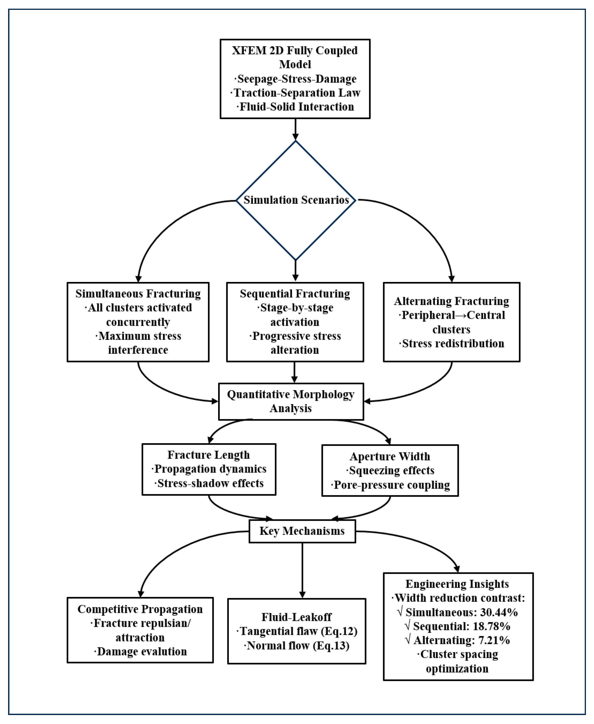
This study advances prior research through a comprehensive 2D fully coupled seepage–stress–damage model based on the Extended Finite Element Method (XFEM). We systematically quantify three fundamental fracturing sequences—simultaneous, sequential, and alternating—comparing their performance in fracture propagation length and aperture width. The work aims to (i) elucidate the mechanistic superiority of alternating sequences in mitigating fracture width reduction and (ii) deliver actionable engineering guidance for optimized stimulation design. Through comparative numerical simulations, the proposed methodology establishes quantitative benchmarks for fracture geometry evolution, providing theoretical foundations for efficient tight gas reservoir development. Scheme 1 is shown as follows:
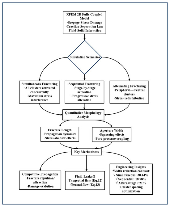
Scheme 1.
Research methodology framework for fracture sequence optimization.
2. Methodology
2.1. XFEM Approximation
The 2D XFEM framework provides superior quantification of fracture geometry (length/aperture width) across three sequencing strategies by (1) isolating near-wellbore stress competition mechanisms governing initial propagation, (2) enabling the computationally efficient parametric analysis of sequencing variables, (3) streamlining the parameterization of planar fracture metrics by eliminating 3D confounding factors, and (4) visually clarifying width reduction patterns under stress interference—collectively establishing high-fidelity benchmarks for sequencing optimization.
In hydraulic fracture simulations, fracture growth is characterized using the Heaviside step function combined with 2D linear elastic asymptotic displacement fields near the fracture tip. This approach permits the arbitrary positioning of fracture discontinuities relative to the base finite element grid, enabling progressive fracture advancement simulations while eliminating remeshing requirements during propagation. The approximation for a displacement vector function u with the partition of unity enrichment is
In this equation, are the standard nodal shape functions, is the nodal displacement vector for the continuous solution domain, signifies the product of the nodal enriched degree of freedom vector. The Heaviside function is represented by and denotes the product of the nodal enriched degree of freedom vector, while corresponds to the fracture-tip functions associated with elastic asymptotic behavior. Crucially, in the XFEM framework, the global nodes preserve the continuous solution term. For fracture-crossing nodes, enrichment with the Heaviside function is essential. Moreover, nodes in close proximity to the fracture tip necessitate asymptotic enrichment to accurately capture the stress intensity factors and ensure the solution’s accuracy near the tip.
are expressed as
The asymptotic tip functions operate within a local polar coordinate system originating at the fracture tip, where aligns with the fracture tangent.
These functions resolve elastostatic crack-tip singularities while accommodating displacement discontinuities across fracture surfaces. Notably, their applicability extends beyond isotropic elastic media.
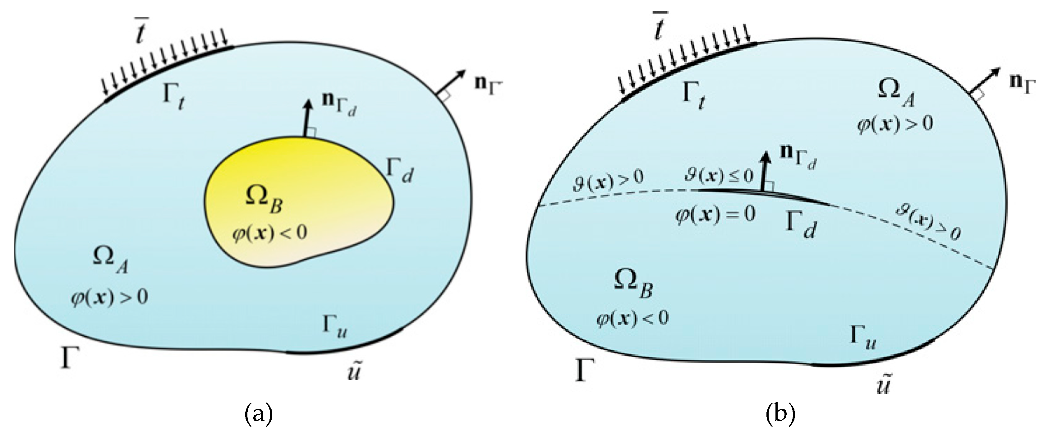
For interface evolution tracking, the level set method represents interfaces as zero-isosurfaces of higher-dimensional functions governed by hyperbolic conservation laws. Consider domain partitioned into subdomains and with interface . As Figure 1 illustrates, closed interfaces traverse entirely (e.g., material boundaries); open interfaces partially penetrate (e.g., crack fronts). The signed distance function provides the most frequent level set representation:
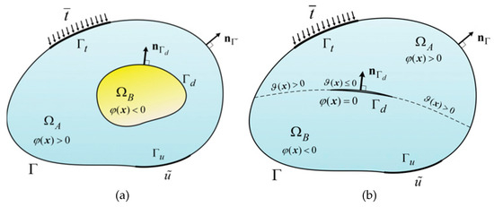
Figure 1.
Phase-field modeling of discontinuities: (a) diffuse interface; (b) sharp crack.
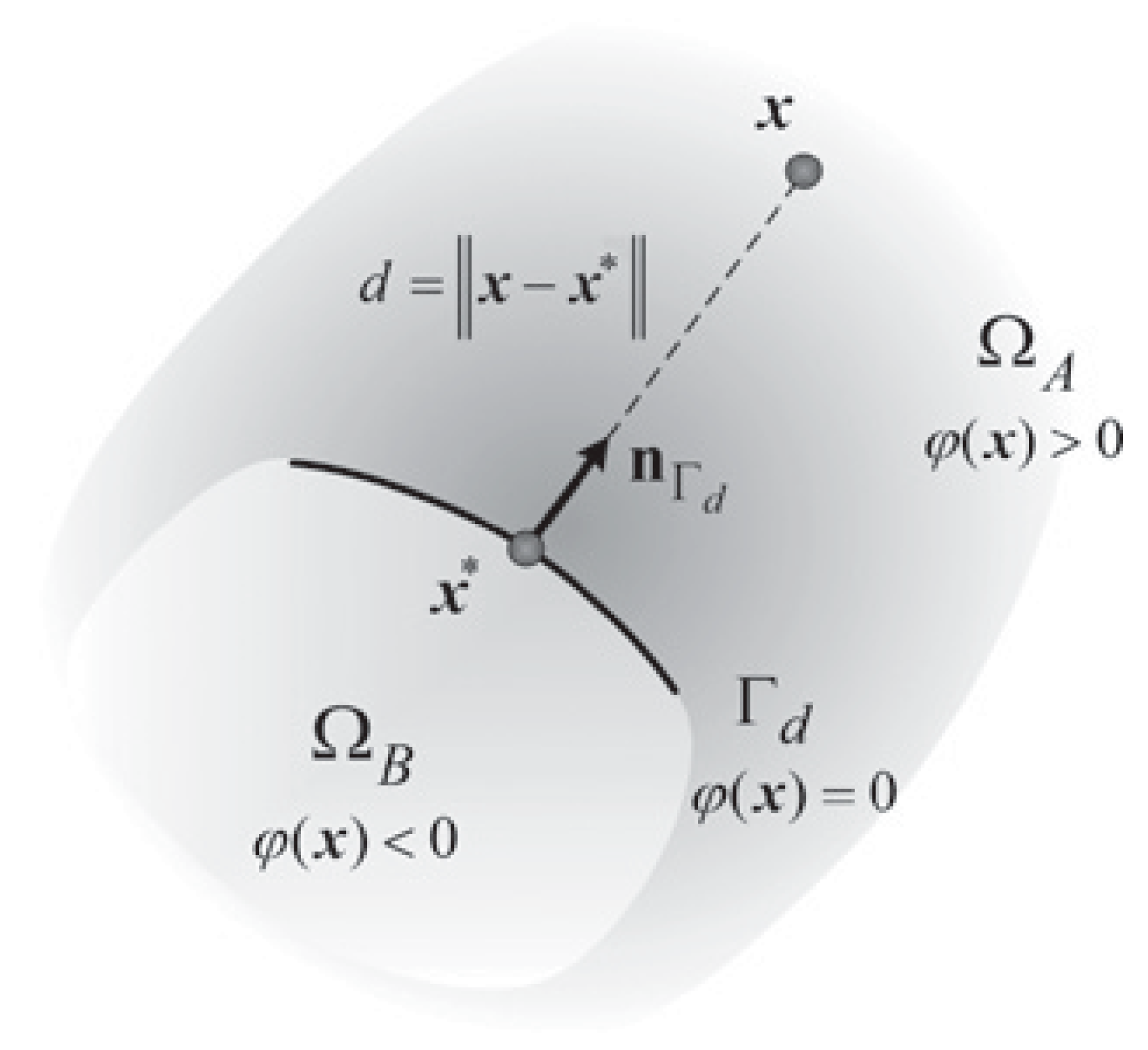
The projection point represents the minimal distance mapping from point to the discontinuity , where denotes the unit normal vector at the projection location . The operator calculates the Euclidean distance, while quantitatively measures the spatial separation between point and the discontinuity boundary .
As mathematically demonstrated in Equation (4), this level set formulation exhibits sign inversion across the closed interface. Consequently, the discontinuity surface Γ can be implicitly characterized by the zero-level isosurface satisfying = 0, which provides
As shown in Figure 2, the displacement field exhibits a sharp discontinuity across crack surfaces, where opposing sides demonstrate fundamentally distinct displacement patterns. This strong discontinuity behavior is mathematically captured in the model through kinematic descriptions employing the Heaviside step function.
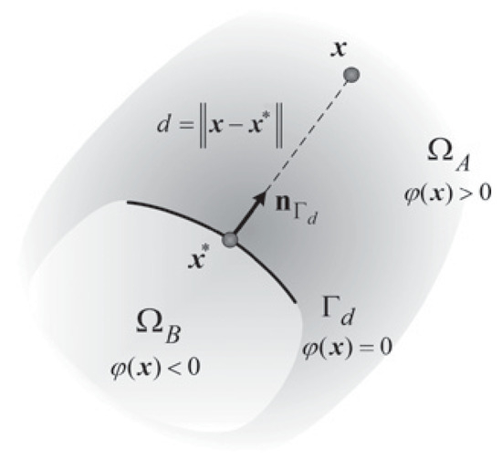
Figure 2.
The signed distance function.
2.2. Modeling Fractures with the Cohesive Zone Method
Linear Elastic Fracture Mechanics (LEFM) establishes its propagation criterion on two fundamental premises: first, the existence of a limited fracture process zone adjacent to the crack tip where non-elastic material behavior remains insignificant relative to overall fracture dimensions; second, the requirement that the applied stress intensity factor surpasses the material’s fracture toughness for crack advancement. This theoretical framework, however, faces limitations when applied to quasi-brittle and ductile materials, where shear-induced plastic deformation near the propagating crack tip often reaches considerable magnitudes. Such pronounced inelastic deformation challenges the validity of LEFM’s core assumptions. Furthermore, the applicability of these assumptions requires careful examination even for nominally brittle materials, particularly when crack-tip behavior is lumped into a single point parameter, as the existence of an initial crack constitutes a fundamental prerequisite for applying Linear Elastic Fracture Mechanics (LEFM). The cohesive zone model is a suitable and simple model for process zone, and for materials that fail by crack growth and coalescence.
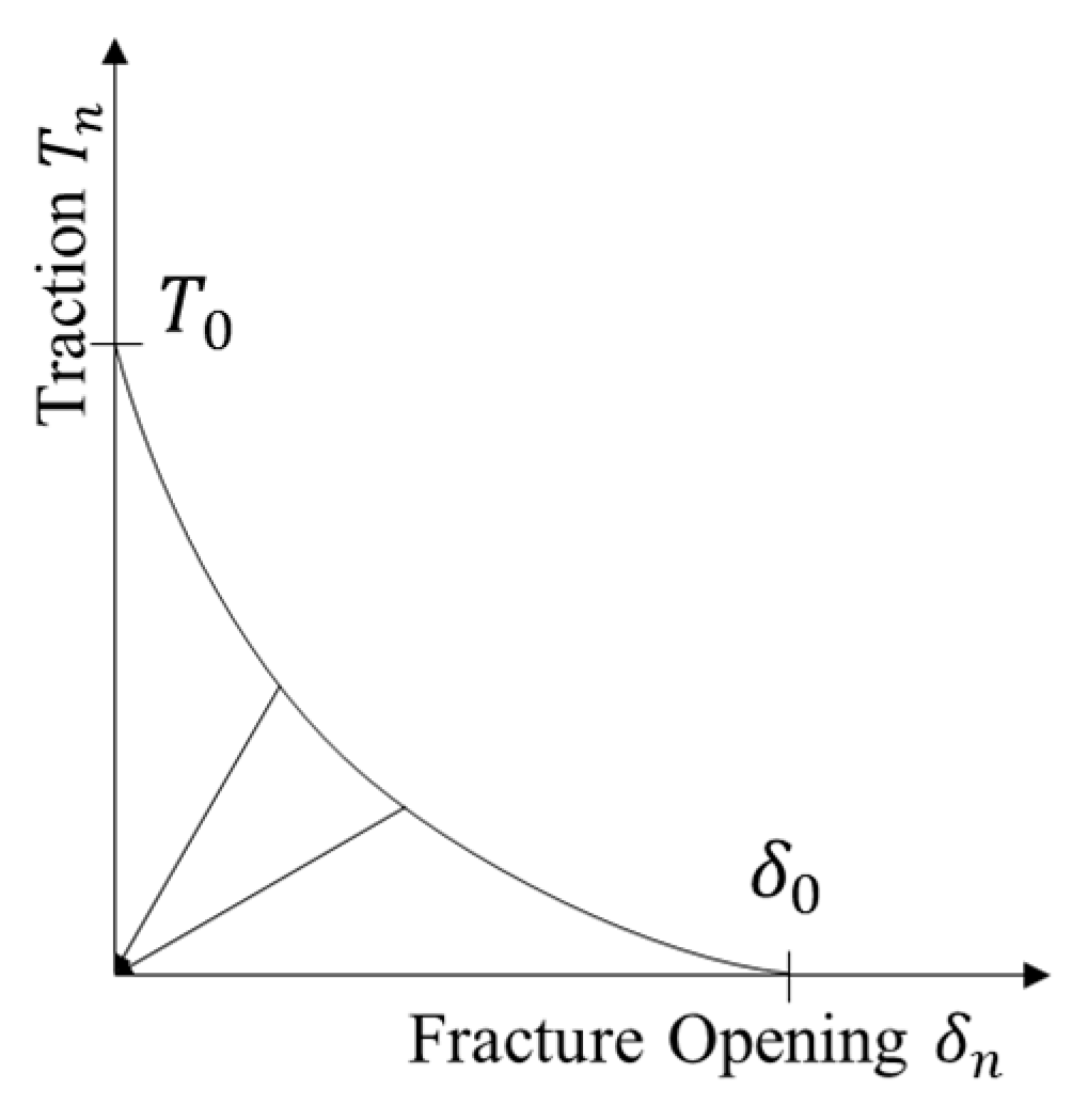
The constitutive behavior of the cohesive zone is defined by the traction–separation relation. The elastic behavior is written in terms of an elastic constitutive matrix that relates the normal and shear stresses to the normal and shear separations of a cracked element.
The interfacial stress state at a material discontinuity can be characterized through vector decomposition: ,, and , comprising orthogonal components that describe both normal and shear stress interactions. The corresponding separations are denoted by , and .
As shown in Figure 3, damage modeling provides an effective framework for simulating the progressive deterioration and ultimate failure of enriched elements. This approach incorporates two fundamental components governing material failure: a criterion determining when damage initiates and a law describing how damage progresses post-initiation. The damage law specifies that elements remain undamaged during pure compressive loading until either the traction attains the cohesive strength threshold or the separation displacement reaches the critical damage value . Beyond this threshold, the traction exhibits linear degradation to zero with increasing displacement, at which point complete failure of the cohesive element occurs.
where, is the stress in the nominal stress, Pa; is the stress in the first shear direction, Pa; is the stress in the second shear direction, Pa; is the peak value stress in the nominal stress, Pa; is the peak value in the first shear direction, Pa; and is the peak value in the second shear direction, Pa. The Macaulay bracket < > in the normal direction signifies that pure compression does not initiate damage.

Figure 3.
Traction–separation law for XFEM.
2.3. Damage Evaluation
The damage evolution law governs the progressive degradation of material stiffness following satisfaction of the initiation criterion. For the present model, this damage progression is mathematically defined as
where D is the overall damage in the material and captures the combined effects of all the active mechanisms. D initially has a value of 0. If damage evolution is modeled, D monotonically evolves from 0 to 1 upon further loading after the initiation of damage. The parameters , and are the stress components predicted by the elastic traction–separation behavior for the current strains without damage.
where .
2.4. Fluid Flow Within the Fractures
In the model, the leakoff of the fracture fluid from the fracture to the matrix was taken into consideration. The analysis adopts the incompressible fluid assumption, with the governing equations derived from a flow continuity principle that accounts for both tangential and normal flow components. According to the Reynold’s equation, the volume flow rate is given by Equations (12) and (13).
Here, q is the flow rate along the tangential direction in the cohesive element, m3/s; d is the gap opening, m; is the pressure gradient along the cohesive element, MPa; is the tangential permeability, 10−3 and μ is the fluid viscosity, mPa·s.
3. Modeling and Simulation
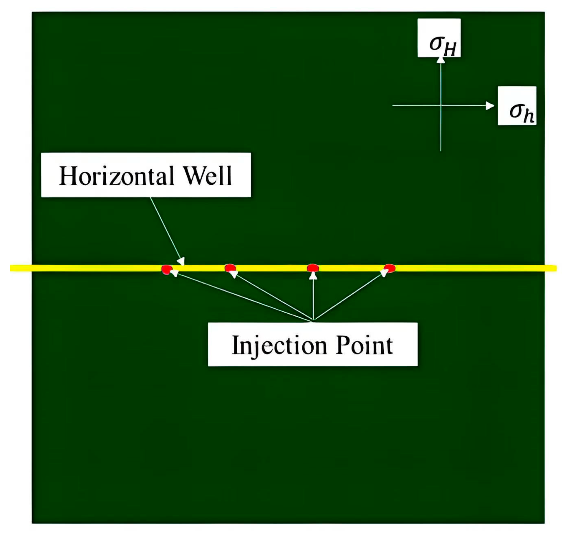
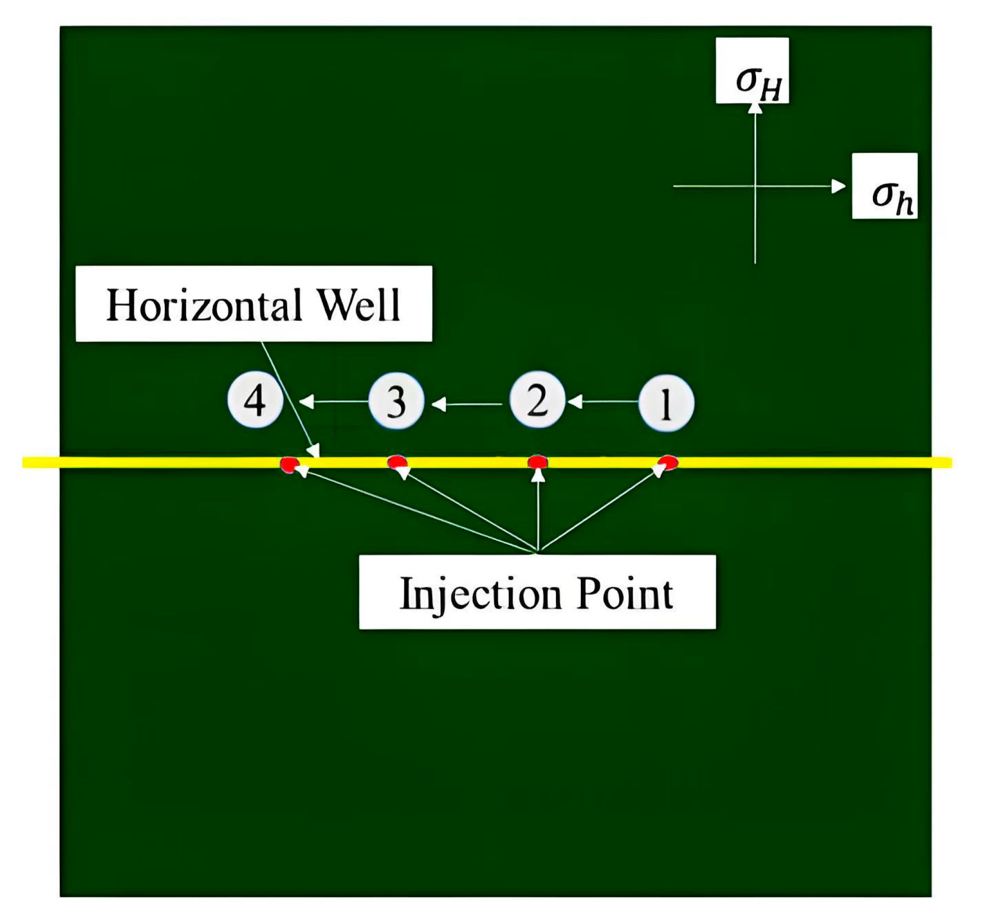
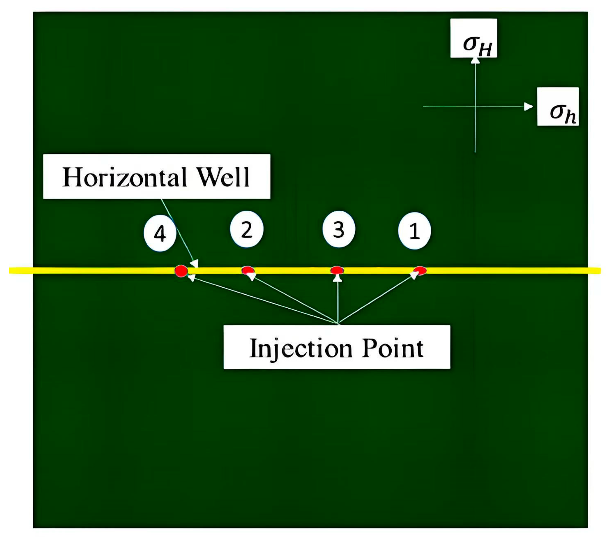
The J5 tight gas reservoir, a continental sedimentary formation with burial depths between 2500 and 3200 m, consists of three distinct lithological units: a 160 meter-thick shale-dominated upper section, a 110 meter-thick sand-shale interbedded middle section, and an 80 meter-thick sandstone-rich lower section serving as the primary target zone. Laboratory analysis of four core samples demonstrated significant mechanical strength, with triaxial compressive strength measurements ranging from 167.92 to 220.01 MPa (mean 184.21 MPa) and Young’s modulus values between 26,110 and 30,045 MPa (average 28,600 MPa), confirming the reservoir’s tight gas characteristics; the Poisson’s ratio varies from 0.198 to 0.248, the average is 0.215. The test results indicated that the compressive strength in this area was very high, and the rock in this reservoir is hard. A finite-element-based sequential fracturing simulation was developed with 180 m dimensions along both wellbore-aligned (X, σhmin-parallel) and transverse (Y, σhmin-perpendicular) axes. The geological model assumed homogeneous sandstone properties without interbedded layers (Figure 4), reflecting the actual sand-dominated reservoir conditions. Hydraulic fracture spacing was parameterized at 30 m intervals.
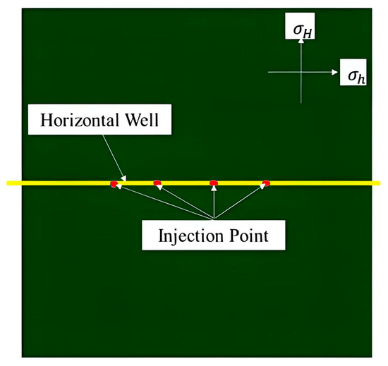
Figure 4.
Sketch of multistage fracture propagation model.
To study the fracture propagation simultaneously, a model with three fracture planes was built. To investigate simultaneous fracture growth, a computational model incorporating three discrete fracture planes was developed. Within this configuration, injection sites corresponded to perforation cluster locations. All simulation parameters are documented in Table 1.

Table 1.
Input parameters for the fracture propagation model.
3.1. Results and Discussion
3.1.1. Simultaneous Fracturing
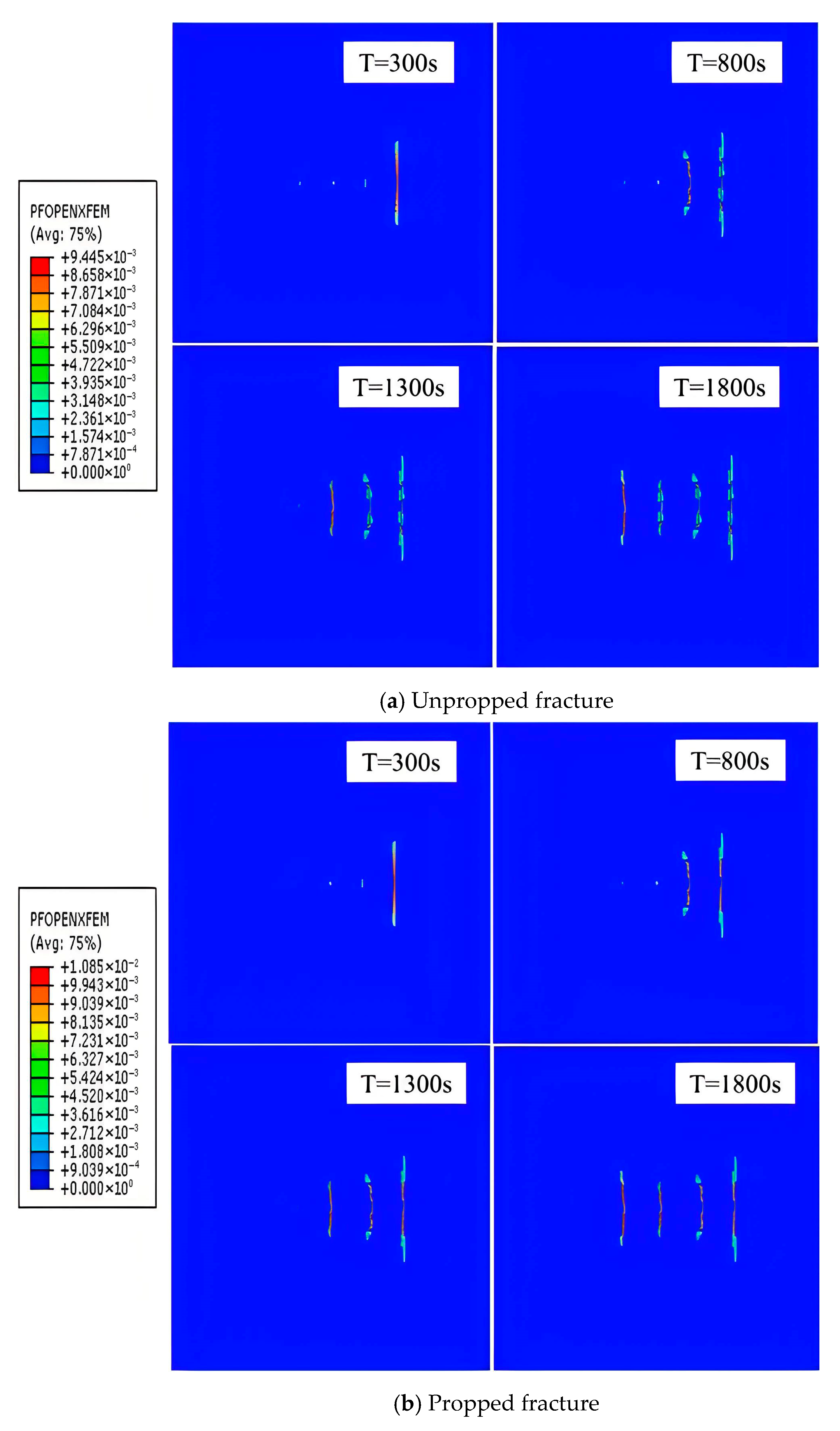
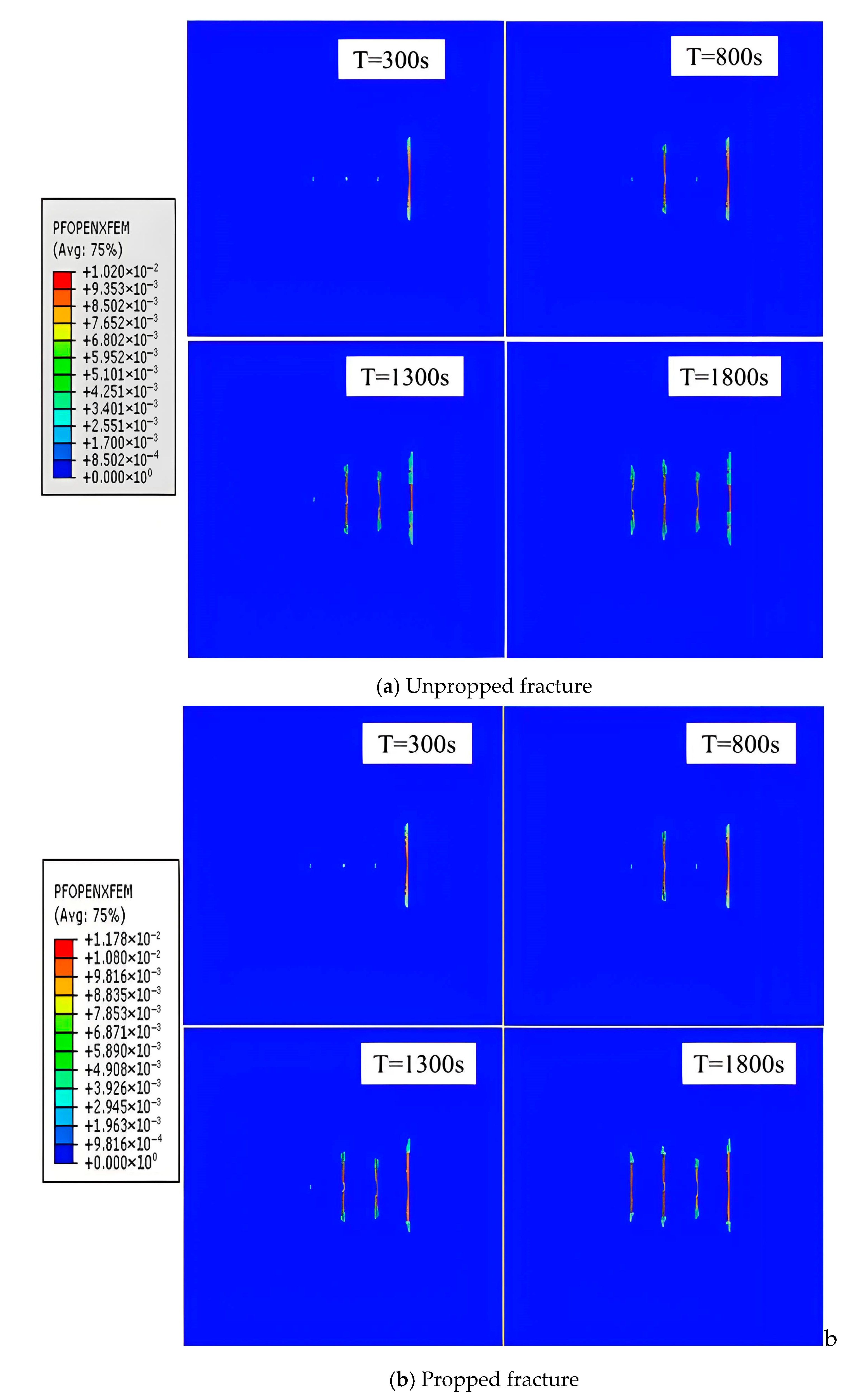
The simultaneous fracturing geometry is shown in Figure 5. Figure 5a, depicts the simultaneous fracturing geometry that is created by unpropped fracturing fluid. The fractures shown are termed as Fracture a, Fracture b, Fracture c, and Fracture d, from right to left. After injection, from 100 s, it is vividly depicted that the middle fractures, for instance, Fracture a and Fracture d, are relatively shorter than the outer fractures (Fracture a and Fracture d). Moreover, all four created fractures propagate along a straight line. However, with the passage of time (after 200 s), the outer fractures deviated from the original maximum principal stress direction during propagation process, while the inner fractures kept their original direction. After a 300 s time period of fracturing fluid injection, the “enwrapped” phenomenon was clearly observed due to the difference in outer and inner fracture lengths. In addition, the outer fracture deviate by 18° from original maximum principal stress direction. The length of four fractures was Fracture a (53 m), Fracture b (38 m), Fracture c (39 m), and Fracture d (54 m). Similarly, Figure 5b illustrated the fracturing propagation as result of injection of propped fracturing fluid. It is also noteworthy that the fracture apertures of all fractures were found to be greater than the fracture created by injection without proppant.
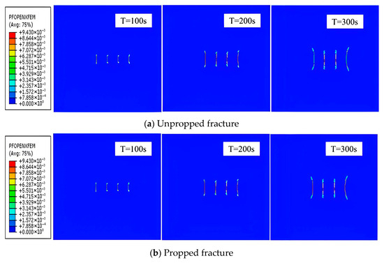
Figure 5.
Fracture geometry of simultaneous fracturing.
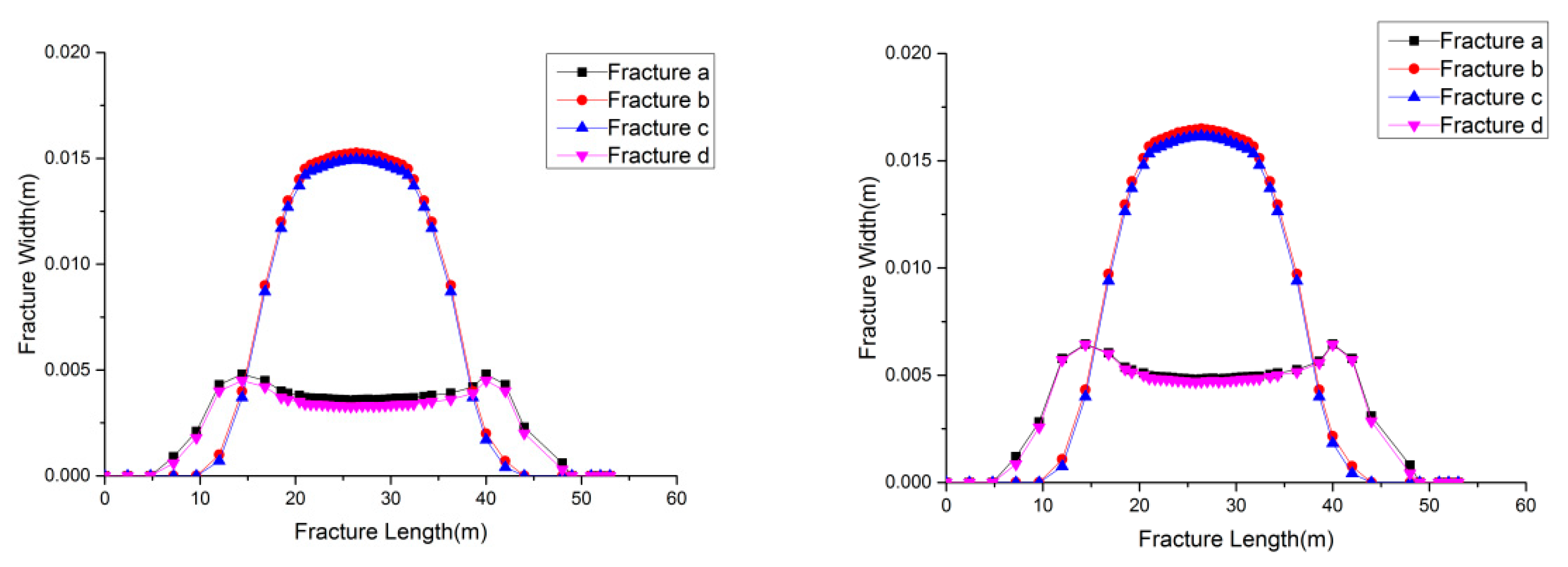
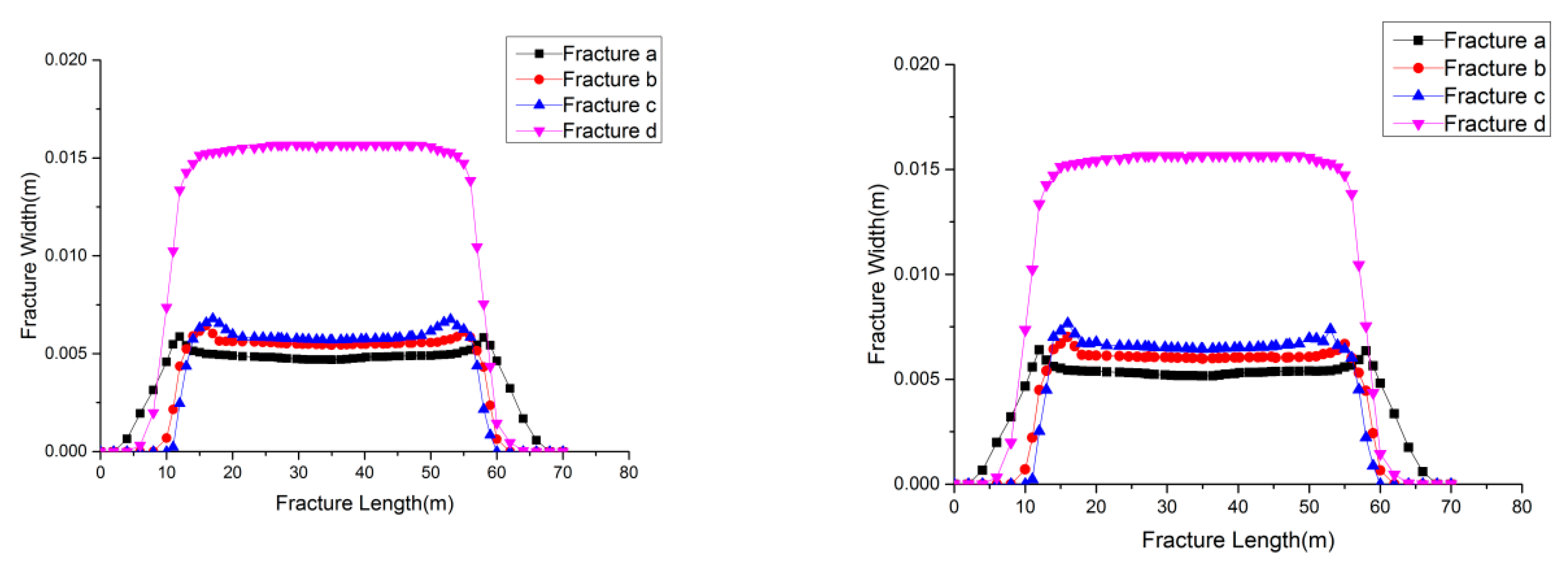
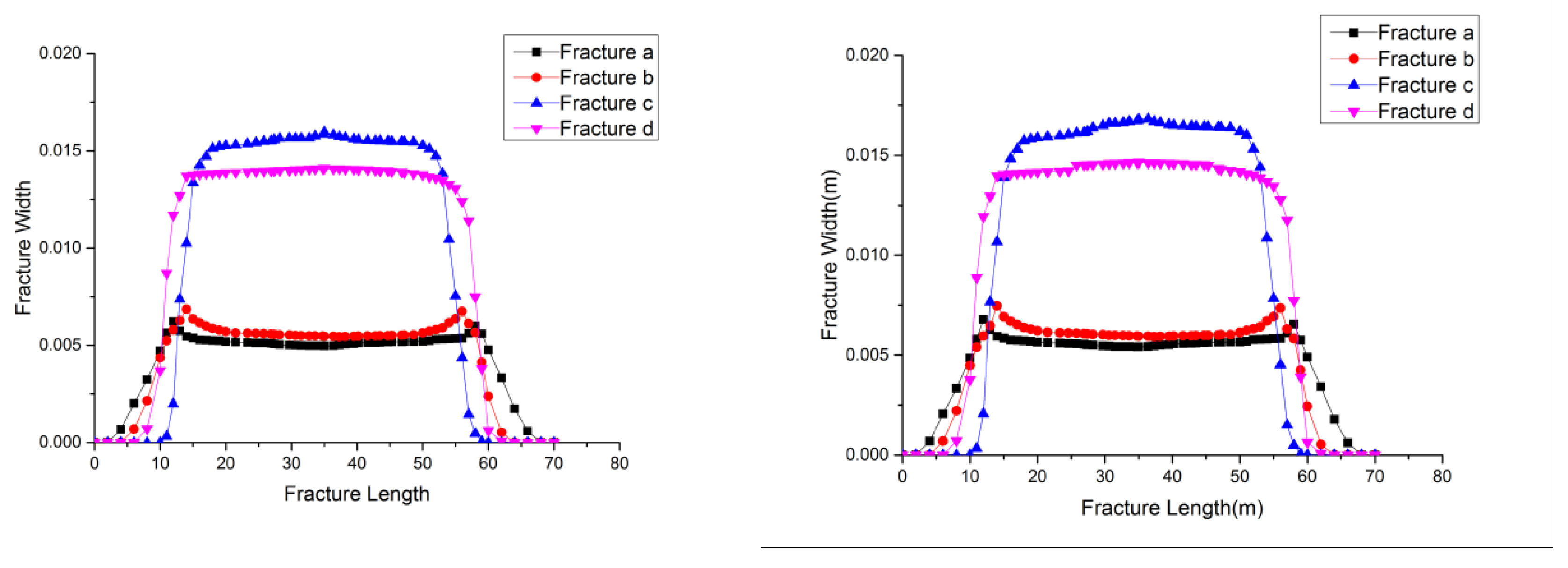
Figure 6 and Table 2 show the plot between fracture width and fracture length. When the proppant was pumped in the schedule, the maximum fracture width of Fracture a increased from 0.0048 m to 0.0062 m, (29.17%), while average fracture width escalated by 32.26% (0.0031 m to 0.0041 m). As far as the Fracture b is concerned, the maximum fracture width went up to 0.0164 m from 0.016 m. In addition, the average fracture width enhanced by 30.0%. Considering fracture c, the maximum fracture width increased from 0.0150 m to 0.0161 m (7.33%). Meanwhile, the average fracture width was found to increase by 25.0%. Lastly, a 31.11% escalation was witnessed in maximum fracture width of Fracture d, while the average fracture width was increased to 0.0039 m from 0.0029 m. It can be concluded from the above outcomes that the width of the outer fracture is far greater than in the inner fractures. On the contrary, the squeezing effect would be more severe in outer fracture than in the inner one.
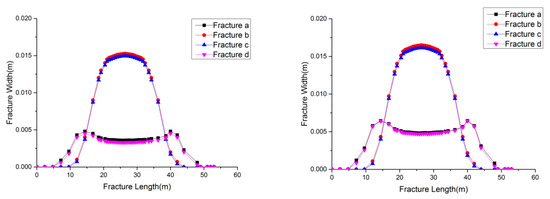
Figure 6.
Fracture width versus fracture length ((Left): unpropped fracture; (Right): propped fracture).
Table 2.
The fracture width of simultaneous fracturing.
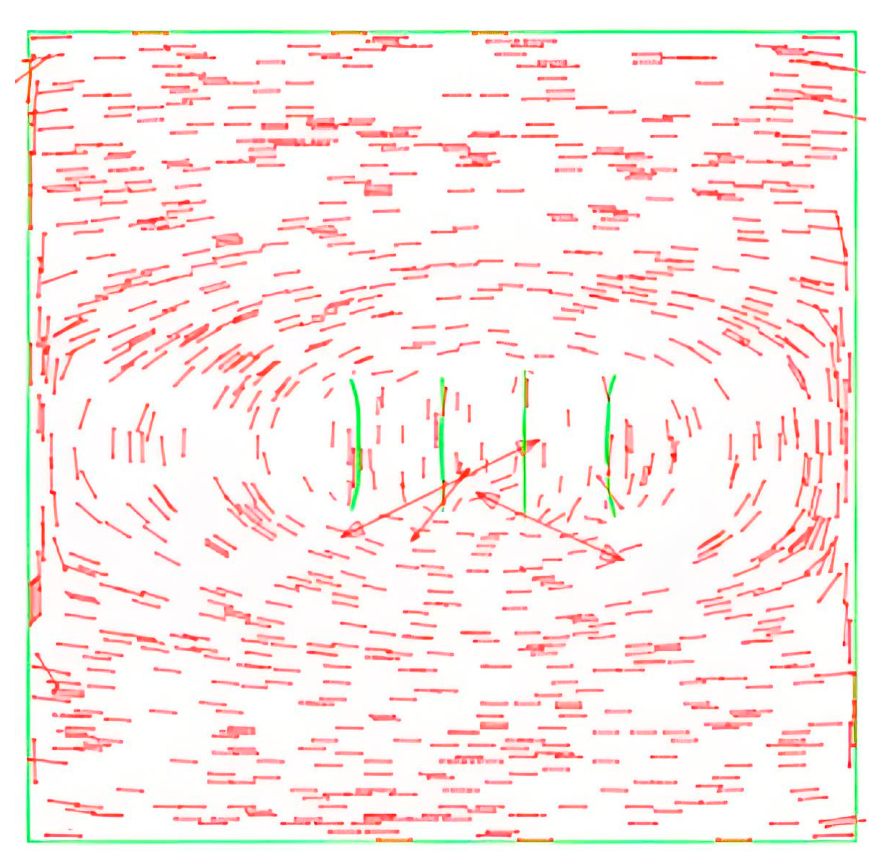
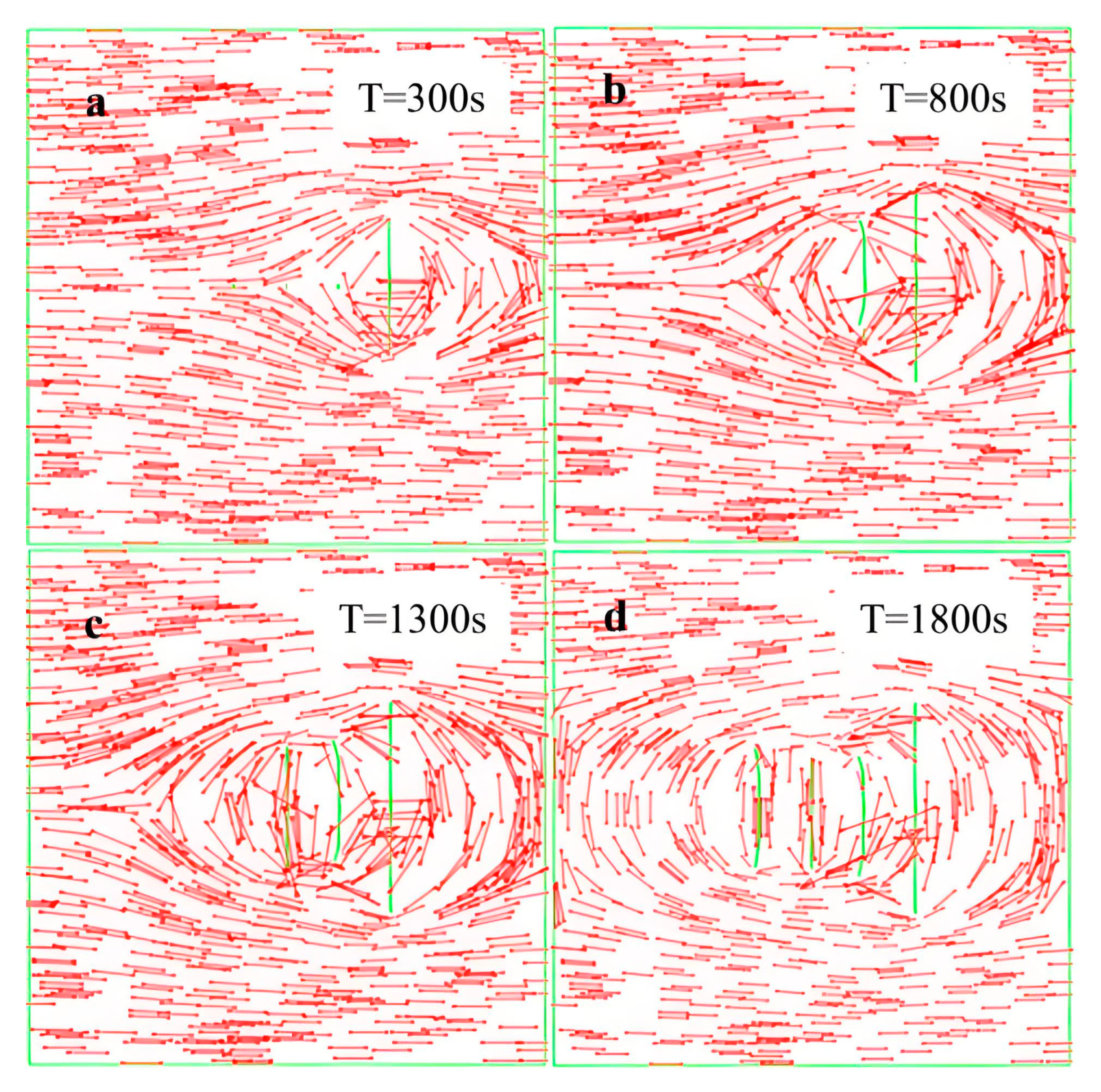
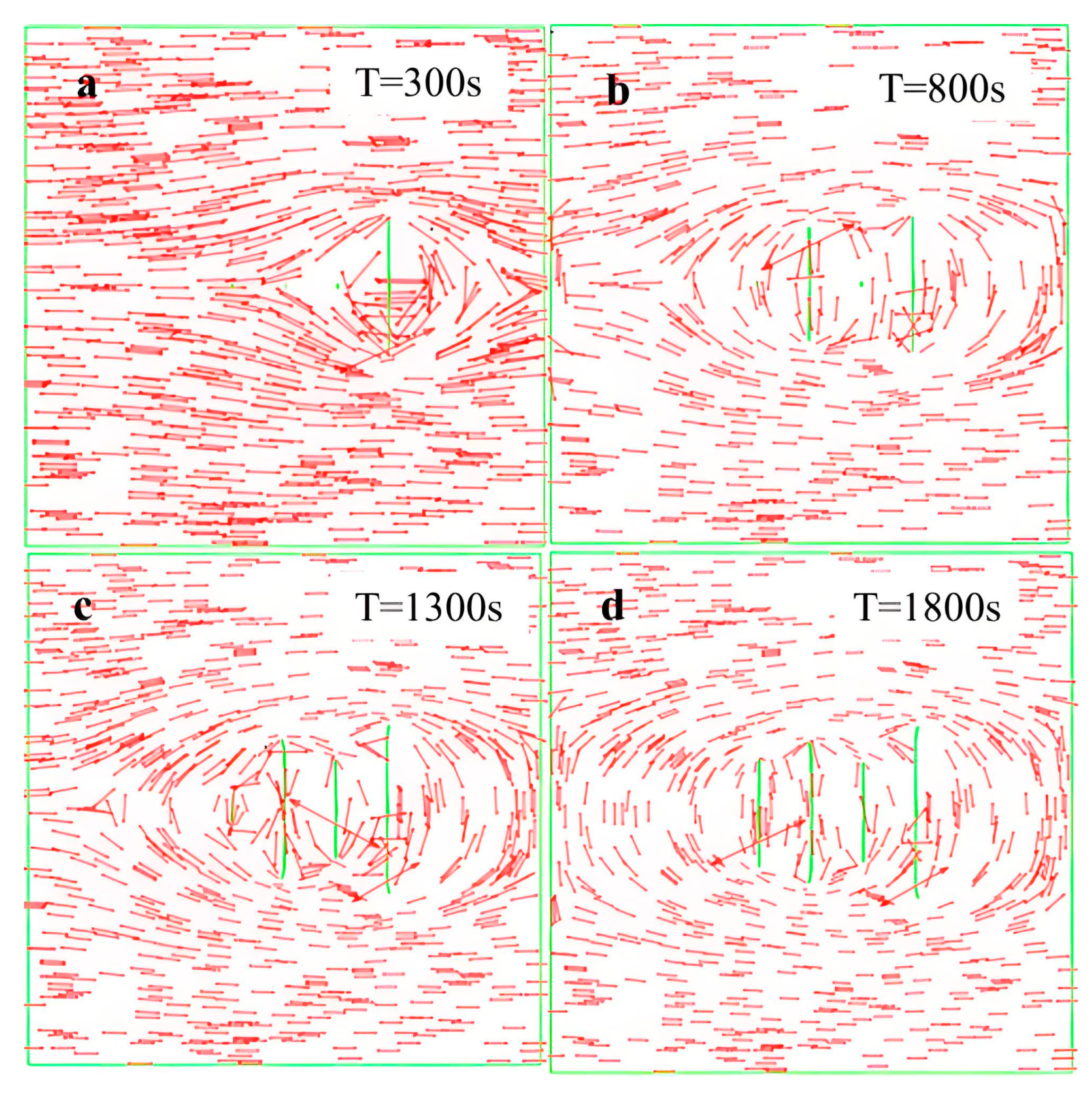
Figure 7 shows the minimum horizontal principle stress distribution after simultaneous fracturing. From the simulation results, it can be concluded that the induced stress field generated by stress deflection was the main reason for outer fracture deflection. In the fracturing process, the hydraulic fractures propagated perpendicular to the minimum horizontal principle stress. The change in minimum horizontal principle stress caused the outer fractures’ deflection. In addition, the propagation of middle fractures generated squeezing effect on the fracture surface under high pumping ratio, which caused the damage degree of outer fractures to be reduced from 200 s to 300 s. When the proppant was pumped in the simulation, the squeezing effect was relieved. When the fracture propagated, the stress deflection also caused the extension pressure rise in middle fracture, which can dramatically shorten the length of the middle fractures. From Figure 7 we can see that there existed an obvious stress concentration at the tip of the middle fractures.
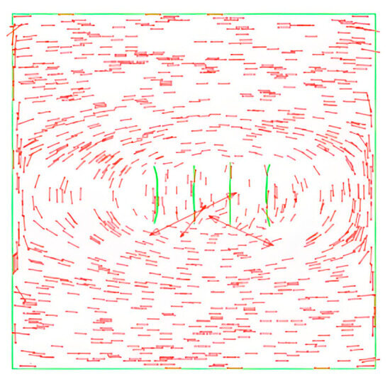
Figure 7.
The minimum horizontal principle stress distribution.
3.1.2. Sequential Fracturing
In this section, the fracture propagation under sequential fracturing (Figure 8) was analyzed. In this simulation, the injection time of every fracture was 300 s and there existed a pumping-off time which was 200 s between two injection schedules. The fractures shown are termed as Fracture a, Fracture b, Fracture c, and Fracture d, from right to left.
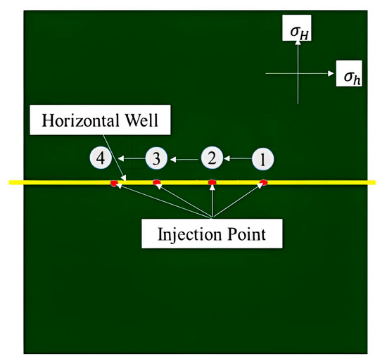
Figure 8.
The schematic diagram of sequential fracturing.
The sequential fracturing geometry is shown in Figure 9. Figure 9a, depicts the sequential fracturing geometry that is created without proppant. The hydraulic fracturing simulation revealed distinct propagation patterns among the four fractures. Initial observations at 300 s showed the linear extension of Fracture a. Subsequent monitoring identified fracture path deviations, with Fracture b developing an 11° deflection from the primary fracture after 200 s of fluid injection, accompanied by noticeable width contraction in Fracture a. By 1300 s of injection, comparative analysis demonstrated that Fracture c exhibited both a shorter extension length (48 m) and smaller deflection angle relative to Fracture b. The propagation process simultaneously induced width reduction in Fracture b. Final injection stage analysis (1800 s) indicated that Fracture d achieved intermediate length (58 m) between Fractures a (64 m) and b/c pair, while displaying greater aperture dimensions than all preceding fractures. Similarly, Figure 9b illustrated the fracturing propagation as a result of the injection of propped fracturing fluid. It is also noteworthy that the fracture apertures of all fractures were found to be greater than the created fracture by injection without proppant.

Figure 9.
Fracture geometry of sequential fracturing.
Figure 10 displays the minimum horizontal principle stress distribution of sequential fracturing. From the simulation results it can be seen that when the first fracture was initiated and propagated, the distribution of the minimum horizontal principle stress had an obvious alteration. The second fracture and the third fracture were within the scope of its influence (as Figure 10a); the alteration of the minimum horizontal principle stress can effectively increase the fracture propagation pressure, which decreased the fracture length. Affected by the induced stress field generated from the minimum horizontal principle stress, there existed a deflection angle when the second fracture propagated (as Figure 10b). In addition, the extension of the second fracture caused a squeezing effect on the fracture surface, which caused the width reduction in first fracture. When the time was 1300 s, because the third fracture was influenced by the induced stress field caused by first fracture and second fracture, the length of the third fracture was shorter than the former two. The extension of the third fracture also made the width reduction in second fracture because of the squeezing effect. Because the influence degree of the induced stress field decreases with the increase in fracture space, the fourth fracture was only affected by the induced stress field caused by second fracture and third fracture. Compared with the induced stress field generated from the first fracture and the second fracture, the induced stress field from the second fracture and third fracture was less than that from the first fracture and the second fracture, which lead the length of fourth fracture to be longer than that of third fracture.
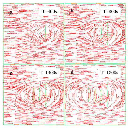
Figure 10.
The minimum horizontal principle stress distribution of sequential fracturing.
Figure 11 and Table 3 show the plot between fracture width and fracture length. When the proppant was pumped in the schedule, the maximum fracture width of Fracture a increased from 0.0059 m to 0.0064 m, (8.95%), while average fracture width escalated by 18.6% (0.0043 m to 0.0051 m). Concerning the Fracture b, the maximum width went up from 0.0064 m to 0.0072 m, and the average fracture width was enhanced by 20.41%. As far as Fracture c, the maximum fracture width was increased from 0.0067 m to 0.0076 m (12.68%). Meanwhile, the average fracture width was found to increase by 28.6%. Lastly, a 3.54% escalation was witnessed in the maximum fracture width of Fracture d, while the average fracture width was increased to 0.0143 m from 0.0133 m. Based on the simulation, taking the Fracture d as the baseline, because there was no squeezing effect on it, the closure pressure was the main reason account for the fracture width reduction in Fracture d. For the fracture a, Fracture b, and Fracture c, the squeezing effect was the main reason accountable for the fracture width reduction. The wider the next fracture was, the stronger the squeezing effect on the last fracture, and the more obvious the reduction in fracture width was.
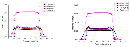
Figure 11.
Fracture width versus fracture length ((Left): unpropped fracture; (Right): propped fracture).
Table 3.
The fracture width of sequential fracturing.
3.1.3. Alternating Fracturing
The scenario of alternating fracturing is seen in Figure 12. In this scheme, the Fracture a was initiated first, then Fracture b was initiated, Fracture c was initiated in the middle of Fracture a and Fracture c, and, at last, Fracture d was initiated. In this simulation, the injection time of every fracture was 300 s and there existed a pumping-off time which was 200 s between two injection schedules.

Figure 12.
The schematic diagram of alternating fracturing.
The alternating fracturing geometry is shown in Figure 13. Figure 13a, depicts the alternating fracturing geometry that is created without proppant. After injection at 300 s and 800 s, Fracture a and Fracture b both propagate along the straight line, but length of the Fracture b was shorter than that of Fracture a. The fracture propagation analysis revealed sequential interactions between multiple fractures. At 1300 s injection time, Fracture c developed between the existing Fractures a and b, achieving intermediate extension (51 m) compared to Fracture b (60 m). This propagation induced noticeable aperture contraction in both adjacent fractures. Subsequent monitoring at 1800 s showed Fracture d forming adjacent to Fracture c, with final dimensions (57 m) intermediate between Fractures b and c. The growth of Fracture d further compressed Fracture c’s aperture. Final measurements recorded fracture lengths as a = 64 m; b = 60 m; c = 51 m; and d = 57 m. Notably, all propped fractures maintained larger apertures than unpropped reference cases. It is also noteworthy that the fracture apertures of all fracture were found to be greater than the created fracture by injection without a proppant.

Figure 13.
Fracture geometry of alternating fracturing.
Figure 14 was the minimum horizontal principle stress distribution of alternating fracturing. From the simulation, the extension of Fracture a altered the minimum horizontal principle stress field, and Fracture b and Fracture c were within the scope of its influence (Figure 14a). When Fracture b propagated, there was an obvious stress concentration at the end of Fracture b. Affected by the diversion of the minimum horizontal principle stress, the extension pressure of Fracture b increased slightly, which caused the extension length of Fracture b to be slightly shorter than Fracture a (Figure 14b). Affected by the diversion of the minimum horizontal principle stress from Fracture a and Fracture b, the stress concentration at the end of Fracture c was much higher than Fracture b, which can dramatically increase the propagation pressure of Fracture c; thus, the extension length of Fracture c was less than Fracture b. In addition, the extension of Fracture c also had a squeezing effect on Fracture a and Fracture b, which made the fracture width of Fracture a decrease significantly; it also caused the reduction in Fracture b (Figure 14c). The extension of Fracture d was affected by the stress diversion from Fracture b, which caused the increase in propagation pressure of Fracture d; so the extension length of Fracture d was shorter than Fracture b.
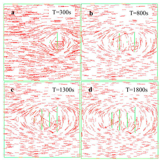
Figure 14.
The minimum horizontal principle stress distribution of alternating fracturing.
Figure 15 and Table 4 shows the plot between fracture width and fracture length. When the proppant was pumped in the schedule, the maximum fracture width of Fracture a increased from 0.0062 m to 0.0068 m (9.68%), while the average fracture width escalated by 9.33% (from 0.0048 m to 0.0052 m). As far as the Fracture b is concerned, the maximum fracture width went up to 0.0074 m from 0.00684 m. In addition, the average fracture width was enhanced by 9.43%. Considering fracture c, the maximum fracture width increased from 0.0159 m to 0.0169 m (6.29%). Meanwhile, the average fracture width was found to increase by 8.33%. Lastly, a 4.29% escalation was witnessed in the maximum fracture width of Fracture d, while the average fracture width was increased to 0.0113 m from 0.0110 m. It can be concluded from the above outcomes that the width of all fractures did not experience an obvious escalation which means that the influence of the squeezing effect was reduced by alternating fracturing.
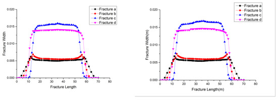
Figure 15.
Fracture width versus fracture length ((Left): unpropped fracture; (Right): propped fracture).
Table 4.
The fracture width of alternating fracturing.
3.2. Analysis
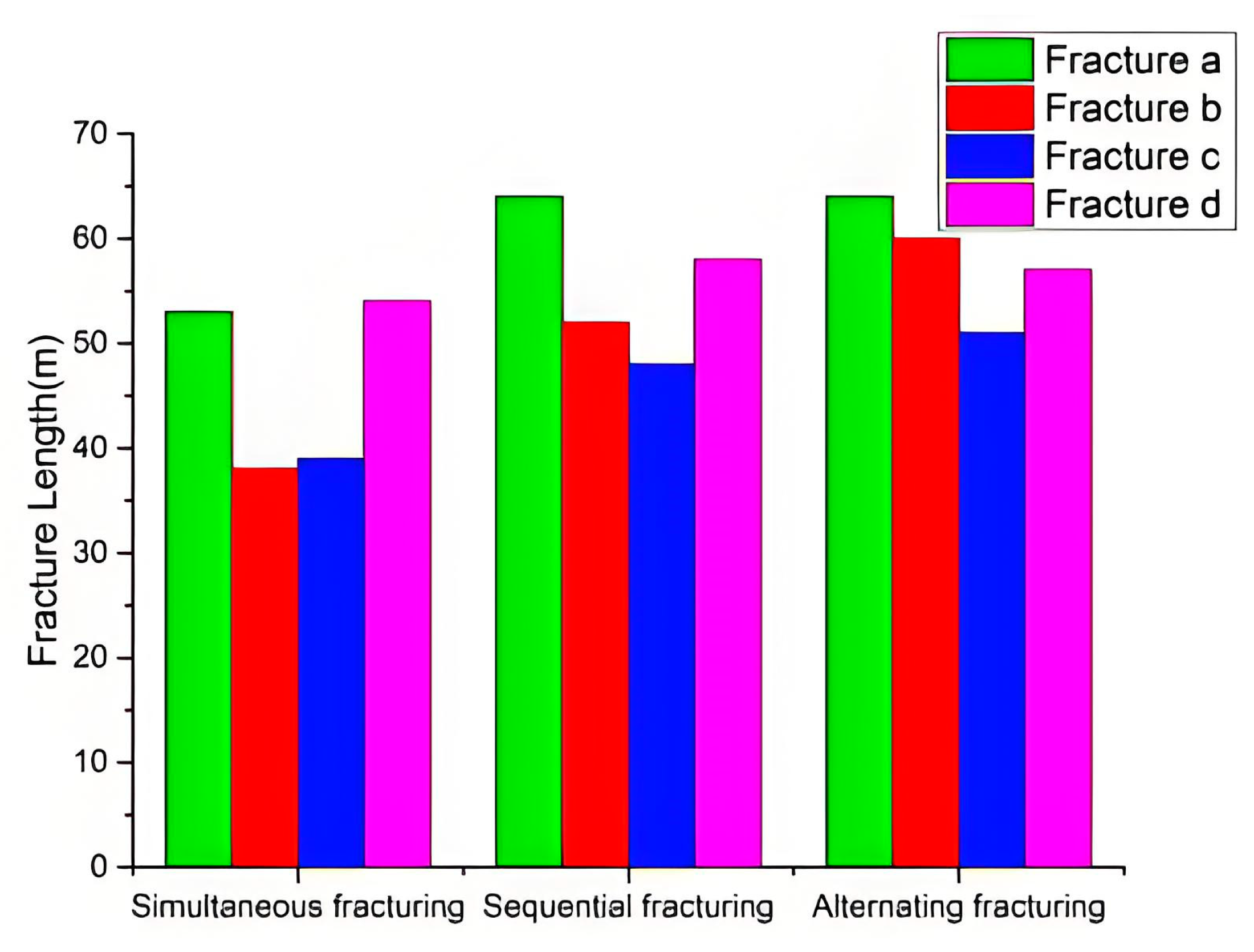
This study presents a comparative analysis of fracture geometries developed through three distinct stimulation methods. Numerical simulations demonstrate that simultaneous fracturing generates fractures measuring 53 m, 38 m, 39 m, and 54 m (total 184 m), while sequential fracturing produces longer extensions of 64 m, 52 m, 48 m, and 58 m (total 222 m). The alternating method proves most effective, yielding fractures of 64 m, 60 m, 51 m, and 57 m (total 232 m), as shown in Figure 16. Results indicate that fracture propagation depends critically on both induced stress fields and initiation sequences, with sequential and alternating methods significantly reducing stress shadow effects to enhance stimulated volume. Notably, alternating fracturing uniquely maintains straight propagation paths, contrasting with the 18° deviations in simultaneous fracturing (Fractures a/d) and 11° deviation in sequential fracturing (Fracture b), while simultaneously mitigating stress-induced deflection. The findings highlight alternating fracturing’s dual advantage in achieving both greater extension length and improved fracture orientation control.

Figure 16.
Fracture length under different fracturing sequence.
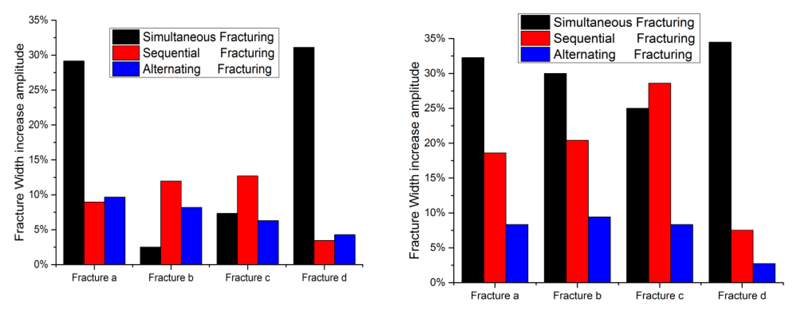
Fracturing sequence not only affected the fracture length but also affected the fracture width. Because the reservoir rock was a porous medium, the squeezing effect caused by the high pumping rate could make the fracture width reduced. The fracture width was the foundation of effective fracture conductivity, which could effectively reduce the flow resistance of oil and gas in the formation. In the simulations, the squeezing effect of simultaneous fracturing can greatly reduce the fracture width. As shown in Figure 17, contrasting the propped fractures and unpropped fractures, the average fracture width increase amplitude was 30.44%, while the average fracture width increase amplitude of sequential fracturing and alternating fracturing were 18.78% and 7.21%, which demonstrated that alternating fracturing was an effective method to guarantee the fracture conductivity in hydraulic fracturing.
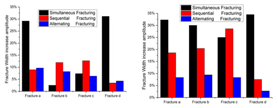
Figure 17.
Fracture length under different fracturing sequence ((Left): the maximum fracture width increase amplitude; (Right): the average fracture width increase amplitude).
4. Conclusions
This study systematically compared three fracturing sequences (simultaneous, sequential, alternating) using a 2D XFEM-based seepage–stress–damage model. The key findings are as follows:
- Fracture Length Enhancement: Sequential and alternating fracturing increased total fracture length by 20.6% (222 m) and 26.1% (232 m), respectively, versus simultaneous fracturing (184 m);
- Width Preservation Superiority: Alternating fracturing minimized pore-pressure-driven squeezing effects, reducing width reduction to 7.21% (vs. 30.44% in simultaneous), optimizing fracture conductivity;
- Deflection Control: Alternating fracturing maintained near-linear propagation (0° deflection), contrasting with 18° and 11° deflections in simultaneous/sequential methods.
Limitations: The 2D homogeneous model neglects lithological heterogeneity and 3D stress interactions.
Future Work: Extend to 3D models incorporating proppant transport and natural fracture networks.
Author Contributions
Conceptualization, Y.T. and H.Z.; methodology, H.Z.; software, Y.T.; validation, J.Z. and Y.T.; investigation, J.Z.; writing—original draft preparation, Y.T.; writing—review and editing, R.L. and H.Z.; visualization, J.Z. and B.S.; supervision, R.L. All authors have read and agreed to the published version of the manuscript.
Funding
This research received no external funding.
Data Availability Statement
The original contributions presented in this study are included in the article. Further inquiries can be directed to the corresponding authors.
Conflicts of Interest
Authors Jin Zhang were employed by the company Xinjiang Oilfield. The remaining authors declare that the research was conducted in the absence of any commercial or financial relationships that could be construed as a potential conflict of interest.
Nomenclature
| XFEM | Extended Finite Element Method |
| LEFM | Linear Elastic Fracture Mechanics |
| CZM | Cohesive Zone Method |
References
- Cheng, Y. Mechanical Interaction of Multiple Fractures—Exploring Impacts of the Selection of the Spacing/Number of Perforation Clusters on Horizontal Shale-Gas Wells. SPE J. 2012, 17, 992–1001. [Google Scholar] [CrossRef]
- Crosby, D.G.; Yang, Z.; Rahman, S.S. Methodology to Predict the Initiation of Multiple Transverse Fractures from Horizontal Wellbores. J. Can. Pet. Technol. 2001, 40, PETSOC-01-10-04. [Google Scholar] [CrossRef]
- Mortazavi, A.; Molladavoodi, H. A numerical investigation of brittle rock damage model in deep underground openings. Eng. Fract. Mech. 2012, 90, 101–120. [Google Scholar] [CrossRef]
- Meyer, B.R.; Bazan, L.W. A Discrete Fracture Network Model for Hydraulically Induced Fractures—Theory, Parametric and Case Studies. SPE Hydraulic Fracturing Technology Conference, The Woodlands, TX, USA, 24–26 January 2011. SPE-140514-MS. [Google Scholar]
- Izadi, G.; Settgast, R.; Moos, D.; Baba, C.; Jo, H. Fully 3D Hydraulic Fracture Growth within Multi-Stage Horizontal Wells. In Proceedings of the 13th ISRM International Congress of Rock Mechanics, Montreal, QC, Canada, 10–13 May 2015. [Google Scholar]
- Guo, J.; Lu, Q.; Zhu, H.; Wang, Y.; Ma, L. Perforating cluster space optimization method of horizontal well multi-stage fracturing in extremely thick unconventional gas reservoir. J. Nat. Gas Sci. Eng. 2015, 26, 1648–1662. [Google Scholar] [CrossRef]
- Barenblatt, G.I. The Mathematical Theory of Equilibrium Cracks in Brittle Fracture. In Advances in Applied Mechanics; Dryden, H.L., von Kármán, T., Kuerti, G., van den Dungen, F.H., Howarth, L., Eds.; Elsevier: Amsterdam, The Netherlands, 1962; pp. 55–129. [Google Scholar]
- Barenblatt, G.I. The formation of equilibrium cracks during brittle fracture. General ideas and hypotheses. Axially-Symmetric cracks. J. Appl. Math. Mech. 1959, 23, 622–636. [Google Scholar] [CrossRef]
- Biot, M.A. Theory of Elasticity and Consolidation for a Porous Anisotropic Solid. J. Appl. Phys. 1955, 26, 4. [Google Scholar] [CrossRef]
- Zhang, G.M.; Liu, H.; Zhang, J.; Wu, H.A.; Wang, X.X. Three-dimensional finite element simulation and parametric study for horizontal well hydraulic fracture. J. Pet. Sci. Eng. 2010, 72, 310–317. [Google Scholar] [CrossRef]
- Turon, A.; Camanho, P.P.; Costa, J.; Dávila, C.G. A damage model for the simulation of delamination in advanced composites under variable-mode loading. Mech. Mater. 2006, 38, 1072–1089. [Google Scholar] [CrossRef]
- Stegent, N.A.; Wagner, A.L.; Mullen, J.; Borstmayer, R.E. Engineering a Successful Fracture-Stimulation Treatment in the Eagle Ford Shale. In Proceedings of the Tight Gas Completions Conference, Society of Petroleum Engineers, San Antonio, TX, USA, 2–3 November 2010. [Google Scholar]
- Sone, H.; Zoback, M.D. Visco-plastic Properties of Shale Gas Reservoir Rocks. In Proceedings of the 45th U.S. Rock Mechanics/Geomechanics Symposium, American Rock Mechanics Association, San Francisco, CA, USA, 26–29 June 2011. [Google Scholar]
- Mokryakov, V. Analytical solution for propagation of hydraulic fracture with Barenblatt’s cohesive tip zone. Int. J. Fract. 2011, 169, 159–168. [Google Scholar] [CrossRef]
- Réthoré, J.; de Borst, R.; Abellan, M.-A. A two-scale model for fluid flow in an unsaturated porous medium with cohesive cracks. Comput. Mech. 2008, 42, 227–238. [Google Scholar] [CrossRef]
- Sheng, M.; Li, G.; Shah, S.; Lamb, A.R.; Bordas, S.P.A. Enriched finite elements for branching cracks in deformable porous media. Eng. Anal. Bound. Elem. 2015, 50, 435–446. [Google Scholar] [CrossRef]
- Gordeliy, E.; Peirce, A. Coupling schemes for modeling hydraulic fracture propagation using the XFEM. Comput. Methods Appl. Mech. Eng. 2013, 253, 305–322. [Google Scholar] [CrossRef]
- Gordeliy, E.; Peirce, A. Implicit level set schemes for modeling hydraulic fractures using the XFEM. Comput. Methods Appl. Mech. Eng. 2013, 266, 125–143. [Google Scholar] [CrossRef]
- Gordeliy, E.; Peirce, A. Enrichment strategies and convergence properties of the XFEM for hydraulic fracture problems. Comput. Methods Appl. Mech. Eng. 2015, 283, 474–502. [Google Scholar] [CrossRef]
- Khoei, A.R.; Haghighat, E. Extended finite element modeling of deformable porous media with arbitrary interfaces. Appl. Math. Model. 2011, 35, 5426–5441. [Google Scholar] [CrossRef]
- Mohammadnejad, T.; Khoei, A.R. An extended finite element method for hydraulic fracture propagation in deformable porous media with the cohesive crack model. Finite Elem. Anal. Des. 2013, 73, 77–95. [Google Scholar] [CrossRef]
- Wu, K.; Olson, J.E.; Balhoff, M.T. Study of Multiple Fracture Interaction Based on An Efficient Three-Dimensional Displacement Discontinuity Method. In Proceedings of the 49th U.S. Rock Mechanics/Geomechanics Symposium, San Francisco, CA, USA, 28 June–1 July 2015. [Google Scholar]
- Wu, K.; Olson, J.; Balhoff, M.T.; Yu, W. Numerical Analysis for Promoting Uniform Development of Simultaneous Multiple Fracture Propagation in Horizontal Wells. In Proceedings of the SPE Annual Technical Conference and Exhibition, Houston, TX, USA, 28–30 September 2015. [Google Scholar]
- Cipolla, C.L.; Lolon, E.P.; Mayerhofer, M.J. Resolving Created, Propped, and Effective Hydraulic-Fracture Length. SPE Prod. Oper. 2009, 24, 619–628. [Google Scholar] [CrossRef]
- Haddad, M.; Du, J.; Vidal-Gilbert, S. Integration of Dynamic Microseismic Data with a True 3D Modeling of Hydraulic-Fracture Propagation in the Vaca Muerta Shale. SPE J. 2017, 22, 1714–1738. [Google Scholar] [CrossRef]
- Guo, T.; Wang, Y.; Chen, M.; Qu, Z.; Tang, S.; Wen, D. Multi-stage and multi-well fracturing and induced stress evaluation: An experiment study. Geoenergy Sci. Eng. 2023, 230, 212271. [Google Scholar] [CrossRef]
- Zhao, H.; Tannant, D.D.; Ma, F.; Guo, J.; Feng, X. Investigation of Hydraulic Fracturing Behavior in Heterogeneous Laminated Rock Using a Micromechanics-Based Numerical Approach. Energies 2019, 12, 3500. [Google Scholar] [CrossRef]
- Chang, C.; Tao, S.; Wang, X.; Liu, C.; Yu, W.; Miao, J. Post-frac evaluation of deep shale gas wells based on a new geology-engineering integrated workflow. Geoenergy Sci. Eng. 2023, 231, 212228. [Google Scholar] [CrossRef]
- Yang, L.; Sheng, X.; Zhang, B.; Yu, H.; Wang, X.; Wang, P.; Mei, J. Propagation behavior of hydraulic fractures in shale under triaxial compression considering the influence of sandstone layers. Gas Sci. Eng. 2023, 110, 204895. [Google Scholar] [CrossRef]
- Yoshioka, K.; Sattari, A.; Nest, M.; Günther, R.-M.; Wuttke, F.; Fischer, T.; Nagel, T. Numerical models of pressure-driven fluid percolation in rock salt: Nucleation and propagation of flow pathways under variable stress conditions. Environ. Earth Sci. 2022, 81, 139. [Google Scholar] [CrossRef]

Disclaimer/Publisher’s Note: The statements, opinions and data contained in all publications are solely those of the individual author(s) and contributor(s) and not of MDPI and/or the editor(s). MDPI and/or the editor(s) disclaim responsibility for any injury to people or property resulting from any ideas, methods, instructions or products referred to in the content. |
© 2025 by the authors. Licensee MDPI, Basel, Switzerland. This article is an open access article distributed under the terms and conditions of the Creative Commons Attribution (CC BY) license (https://creativecommons.org/licenses/by/4.0/).