A Short-Term Electricity Load Forecasting Method Based on Multi-Factor Impact Analysis and BP-GRU Model

Abstract

In response to the challenges faced by traditional short-term electricity load forecasting models during holiday load predictions, a novel approach based on multifactor analysis and the Backpropagation–Gated Recurrent Unit (BP-GRU) model is proposed. Firstly, the impacts of temperature, humidity, and the type of date on the electricity load curve are examined. The study clarifies the positive and negative effects of temperature at different times on load forecasting and reveals the non-dependence characteristics of historical data on holiday load curves. Secondly, the performance of various model weight parameter optimization algorithms is assessed, leading to the establishment of a combined GRU and BP model. The operational workflow of the BP-GRU model is introduced. Lastly, the effectiveness of the proposed forecasting model is verified using actual load data. Compared to existing models, the proposed approach exhibits a significant advantage in achieving higher accuracy in holiday load predictions.

1. Introduction

Electric power is a fundamental pillar of modern society, driving industrial production, commercial activities, and daily life [1,2]. With the rapid growth of urbanization, industrialization, and the increasing integration of renewable energy sources, power systems are facing unprecedented challenges in maintaining a stable and efficient supply–demand balance. Historically, electricity demand has exhibited complex patterns influenced by various factors, including economic development, seasonal variations, weather conditions, and consumer behavior. The inherent uncertainty and volatility of power consumption make accurate load forecasting a critical task for energy management.

Power load forecasting plays a pivotal role in ensuring the reliability, sustainability, and economic efficiency of power systems. Accurate predictions enable utility companies to optimize generation schedules, reduce operational costs, and minimize energy waste, thereby supporting the transition toward smart grids and sustainable energy practices. Short-term load forecasting (STLF) aids real-time grid management, while medium- and long-term forecasting facilitates infrastructure planning and investment decisions. Furthermore, with the increasing adoption of intermittent renewable energy sources such as wind and solar, precise load forecasting becomes even more essential to balance supply with demand and enhance grid stability.

Currently, electricity load forecasting is primarily achieved through artificial intelligence models. Kong and colleagues employed a Long Short-Term Memory (LSTM) neural network model to perform localized load forecasting for individual users using metered data [3]. Li et al. proposed a combined load forecasting model that integrates a Convolutional Neural Network (CNN) and Long Short-Term Memory (LSTM) with a salp swarm algorithm optimization and an attention mechanism [4]. Shang et al. proposed a multivariate multi-aggregation model combining CNN and LSTM to achieve short-term electricity load forecasting [5]. Abumohsen et al. conducted research on electricity load forecasting using models such as LSTM [6]. In addition to the LSTM model, some researchers have employed simpler BP (Backpropagation) neural networks for load forecasting. Wang et al. utilized a cat swarm optimization algorithm to enhance the BP neural network model and conducted a study on short-term electricity load forecasting [7]. Aribowo proposed an approach for electricity load forecasting using a cascading feedforward BP neural network. This method accommodates nonlinear conditions while still considering linear factors [8]. Eskandari et al. proposed a load forecasting model that combines CNN and Recurrent Neural Networks (RNN). The model uses the CNN for feature extraction, followed by the RNN to produce the load forecast values [9].

Concurrently, some researchers have improved the gated recurrent unit (GRU) neural networks and applied them to load forecasting. For instance, Deng et al. developed a predictive method that combines ensemble empirical mode decomposition with GRU and multiple linear regression [10]. Li et al. proposed a sparrow search optimization algorithm to enhance a GRU neural network model, addressing the issue of modal aliasing in historical data [11]. Wang et al. introduced a new “sequence-to-sequence” architecture based on a dual attention mechanism and bidirectional gated units, which enhances the accuracy of load forecasting [12]. Additionally, some researchers have combined GRU with other machine learning algorithms to create hybrid models that achieve load forecasting under various conditions [13,14,15,16,17]. They leveraged the time-series processing capability of GRU networks, enabling historical data to effectively inform current load forecasting.

The aforementioned research successfully achieved accurate predictions of electrical load under typical conditions. However, during certain statutory holidays, most businesses, government agencies, schools, and other institutions are closed, resulting in a significant drop in electricity consumption. Consequently, the load curves during these periods differ markedly from those observed on weekdays and weekends, which undermines the accuracy of time series forecasting methods that rely on recent historical data. To address the aforementioned issue, this paper proposes a short-term electricity load forecasting model based on multi-factor influence analysis and BP-GRU, enabling accurate predictions of electricity consumption during holidays.

The contributions of this paper are summarized as follows:

(1) The effects of temperature, humidity, rainfall, and date type on the electricity load curve were analyzed. The findings revealed the positive influence of temperature in both summer and winter, contrasted by its negative impact during spring and autumn. Low-correlation factors such as humidity and rainfall were excluded. Additionally, various patterns of change in the electricity load curve were clearly identified for weekdays, weekends, and holidays.

(2) Multiple algorithms for adjusting weight parameters in neural networks were assessed, leading to the development of a combined BP-GRU neural network model. This model adeptly integrates temperature factors based on human comfort assessments, thereby avoiding their adverse effects.

(3) The proposed load forecasting model was validated through the selection of various typical daily load data points, including those from weekdays and holidays, to evaluate its predictive capability. Furthermore, evaluation metrics such as MAPE, MAE, and RMSE were established to reflect the model’s errors from multiple perspectives. This paper also conducted a comparative analysis with several existing models to emphasize the advantages of the proposed mode.

The remainder of this paper is organized as follows. The Section 2 analyzes the impact of various factors on electricity load. The Section 3 proposes a methodology for short-term electricity load forecasting. The Section 4 verifies the effectiveness and advancement of the proposed method. The Section 5 summarizes the entire paper.

2. Analysis of Factors Affecting Electricity Load Forecasting

The original data studied in this paper includes historical load, temperature, humidity, and rainfall. Each feature has varying relevance to electricity load forecasting under different conditions. Therefore, this section conducts comparative experiments to analyze the impact of these different features. Additionally, this study utilizes competition data from China’s “Electrician Cup” National College Mathematical Modeling Contest. The dataset consists of 105,600 data points collected at 15 min intervals. The dataset was partitioned as follows: 70% for training, 20% for testing, and 10% for validation.

2.1. Temperature

According to the conclusions drawn from reference [18], when the weight of temperature as a factor is relatively low, it is possible to achieve higher accuracy in electricity load forecasting even in the presence of weather-sensitive loads, without considering temperature. This is because, in ultra-short-term electricity load forecasting, the historical data points are very close in time to the prediction point (15 min apart). Temperature changes within a 15 min window are minimal, and the temperature influences captured in recent historical data can provide valuable insights for predicting load 15 min ahead. Therefore, there are many instances in ultra-short-term forecasting where using only historical data can lead to higher accuracy.

However, in this study’s short-term electricity load forecasting, the historical data points are significantly farther from the prediction time (up to 24 h), making it difficult for temperature influences reflected in recent history to provide any relevant insights for load forecasting several hours later. Consequently, temperature becomes theoretically more important for load forecasting in this context. This section examines one representative date from each season: spring, summer, autumn, and winter.

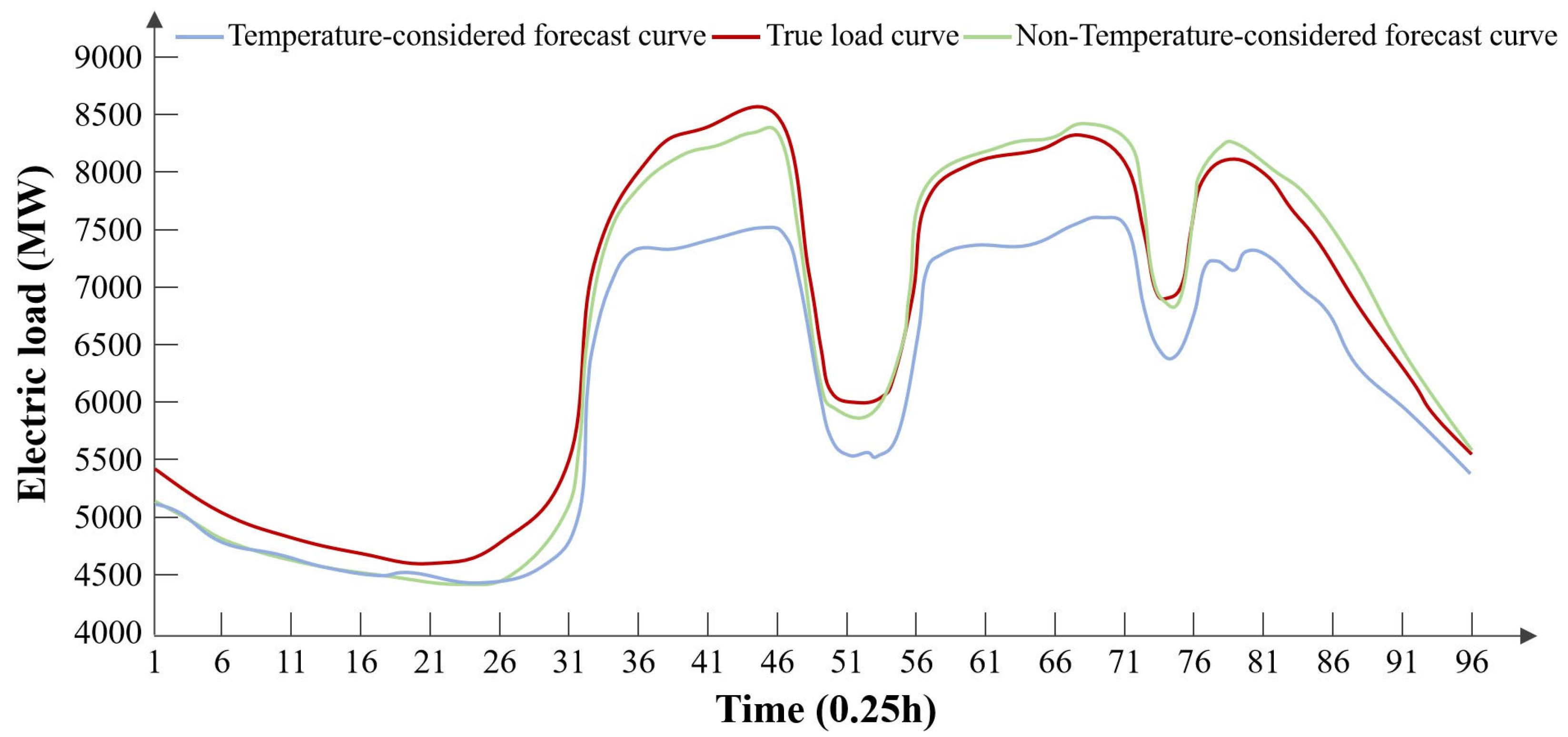
An experimental study on load forecasting for a typical spring day was conducted, and the results are presented in Figure 1 and

Table 1. Table of error metrics for temperature comparison experiments on a typical spring day.

Error Metrics	Considering Temperature	Not Considering Temperature
MAPE	7.040%	2.596%
MAE	484.041	151.592
RMSE	522.646	170.925

.

From the comparison of experimental results, it can be concluded that in spring, temperature cannot be considered a feature for electricity load forecasting. Taking temperature into account has a negative impact on electricity load predictions.

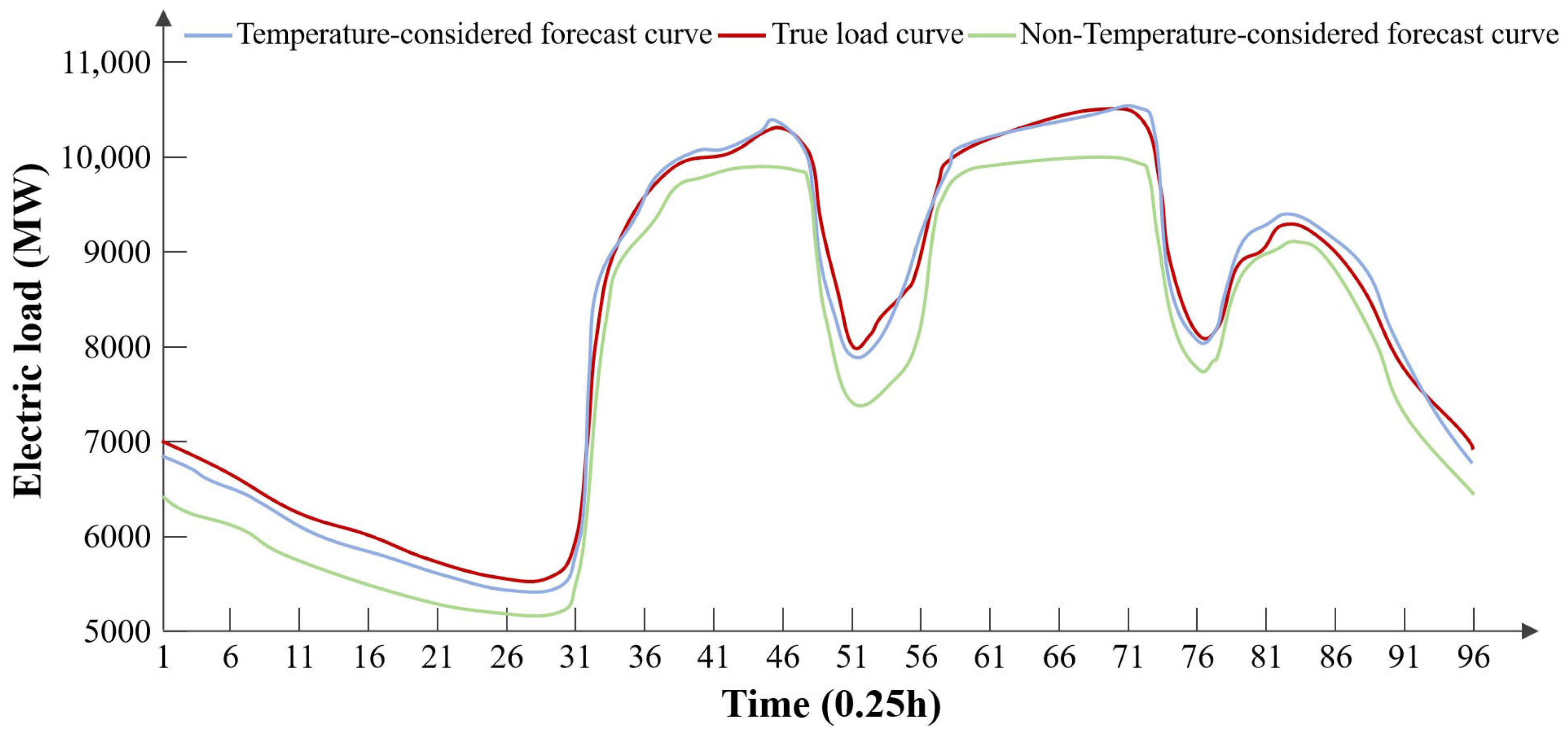
For a typical summer day, the comparison results are shown in Figure 2 and

Table 2. Error metrics results of the temperature comparison experiment for a typical summer day.

Error Metrics	Considering Temperature	Not Considering Temperature
MAPE	1.381%	6.148%
MAE	101.295	479.413
RMSE	120.931	498.878

. In summer, the experimental results indicate that considering temperature factors have a positive impact on electricity load forecasting.

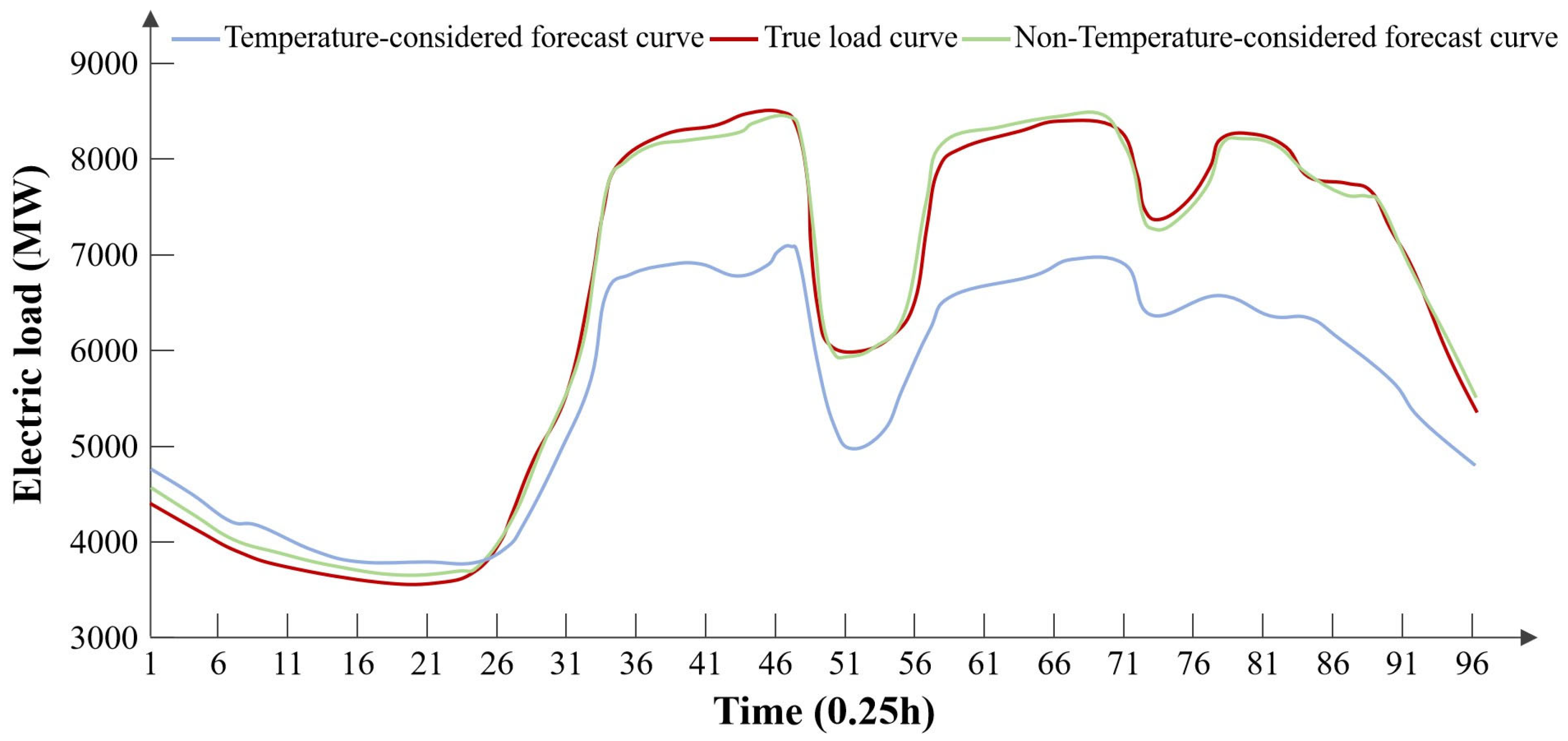
The comparison experiment results for a typical autumn day are shown in Figure 3 and

Table 3. Error metrics results of the temperature comparison experiment for a typical autumn day.

Error Metrics	Considering Temperature	Not Considering Temperature
MAPE	13.498%	1.240%
MAE	959.499	69.653
RMSE	1131.740	78.861

. The experimental results indicate that in autumn, considering temperature reduces the accuracy of electricity load forecasting.

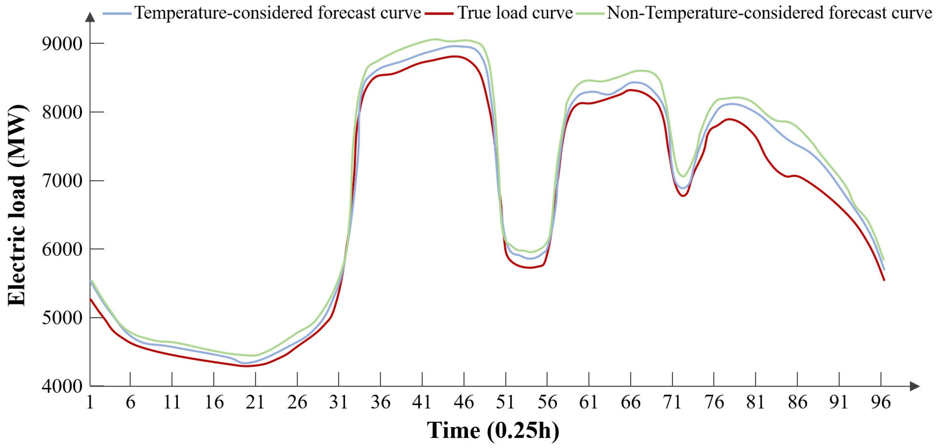
The research on a typical winter day, along with the comparison experiment results, is shown in Figure 4 and

Table 4. Error metrics results of the temperature comparison experiment for a typical winter day.

Error Metrics	Considering Temperature	Not Considering Temperature
MAPE	1.896%	3.270%
MAE	120.611	208.447
RMSE	131.238	221.546

. The experimental results indicate that in winter, considering temperature factors positively contributes to electricity load forecasting.

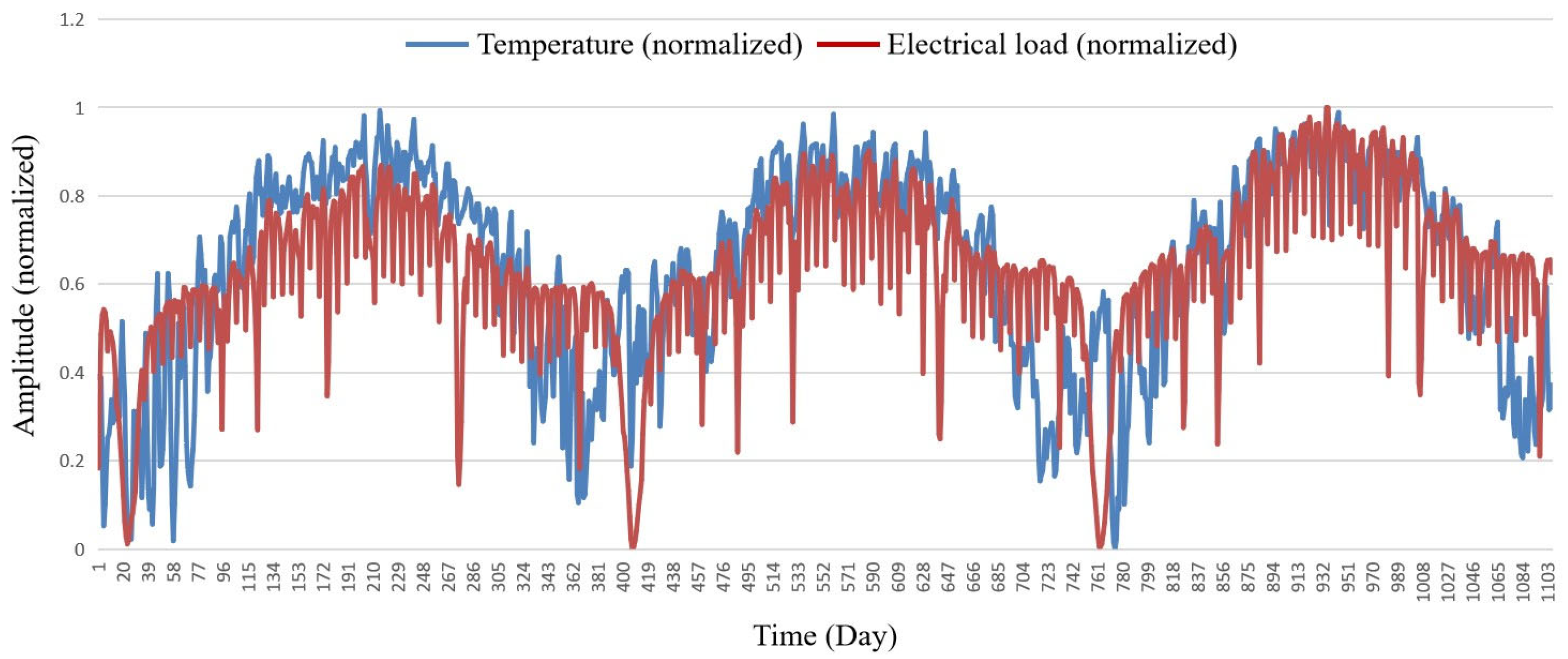
We present a graph illustrating the variation in temperature and electricity load over time, as shown in Figure 5.

Overall, the temperature trend is similar to that of electricity load, with a correlation coefficient of 0.6378. In summary, during periods of higher temperature-sensitive loads, such as summer and winter, temperature characteristics help improve the accuracy of electricity load forecasting. Conversely, during spring and autumn, when the proportion of temperature-sensitive loads is lower, temperature characteristics may negatively impact load predictions. Overall, there is a high correlation between temperature and electricity load; thus, for short-term electricity load forecasting, the consideration of temperature can be decided based on actual conditions.

2.2. Humidity

This section sets up two groups of models for the experiment. The first group considers temperature, humidity, rainfall, and historical load factors; the second group considers only temperature and historical load factors. Since there is a dependent relationship between humidity and rainfall—rainfall will only be greater than zero when humidity exceeds a certain threshold—humidity and rainfall factors are bound together in this experiment. Data from two typical days are tested in this section, with results shown in

Table 5. Results of humidity comparison experimental.

Test Date	Experimental Setup	MAPE	MAE	RMSE
Typical Day 1	Considering Humidity	2.037%	145.740	186.096
	Not Considering Humidity	1.474%	118.463	166.769
Typical Day 2	Considering Humidity	4.755%	405.761	483.597
	Not Considering Humidity	2.170%	156.192	181.346

.

Additionally, we examined the correlation between humidity, rainfall, and electricity load in the region.

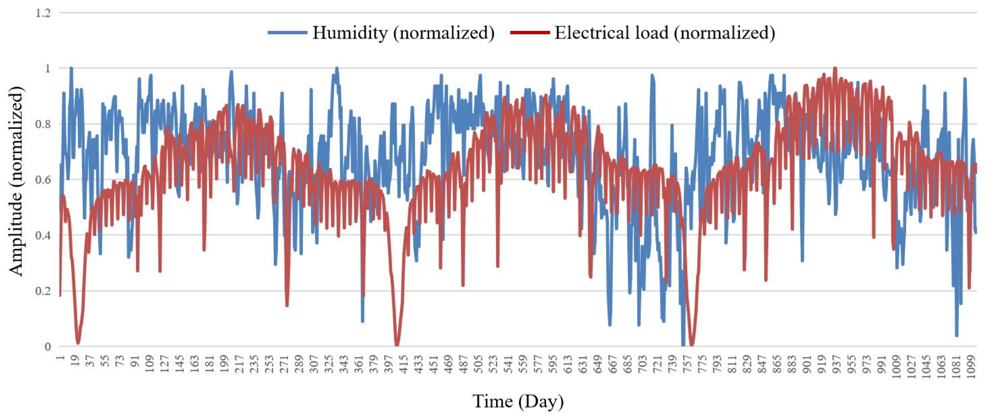
Study on the Correlation Between Humidity and Electricity Load. To investigate the overall relationship between humidity and electricity load, we conducted a correlation analysis using all available data for both variables. The results are presented in Figure 6. The calculated correlation coefficient between humidity and electricity load is 0.1152, indicating a weak correlation. From the figure, it can be observed that electricity load changes exhibit a certain degree of periodicity, whereas humidity changes appear to be more random, showing an unclear correlation between the two.

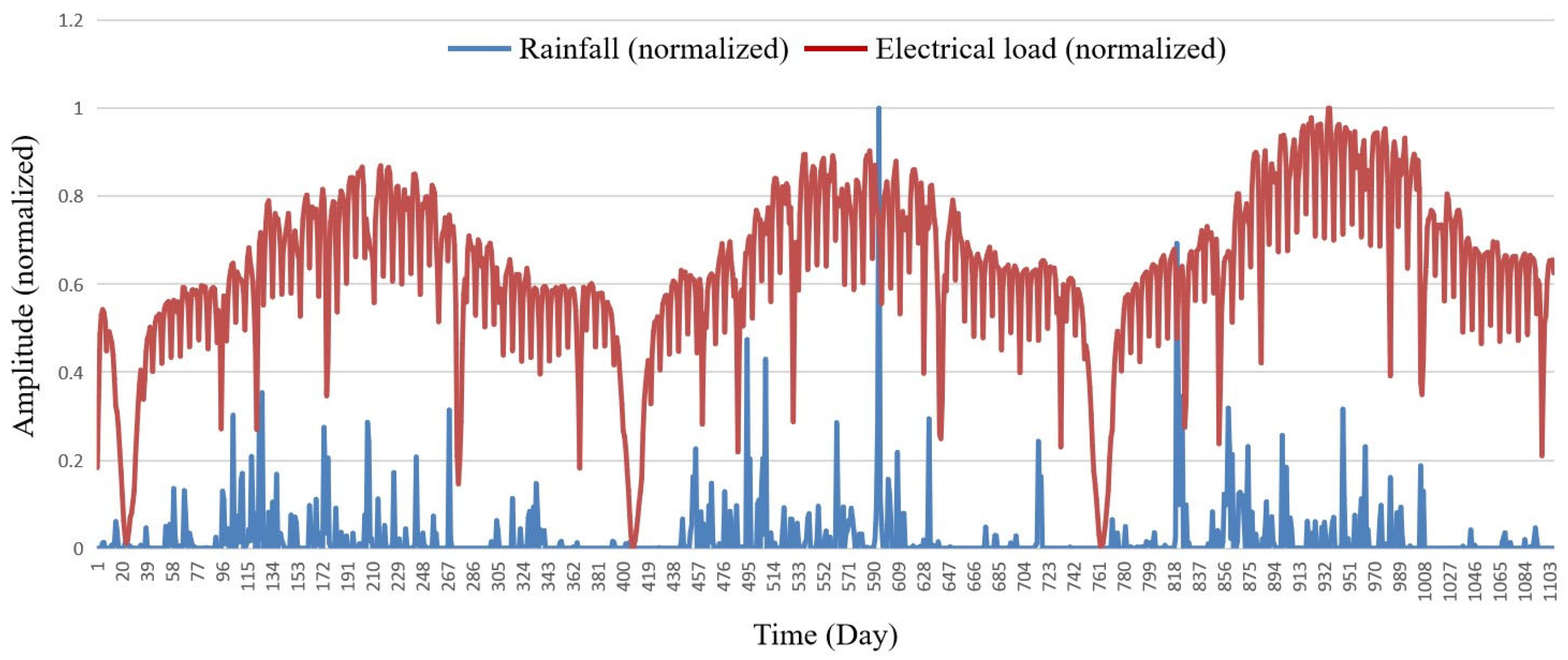
Study on the Correlation Between Rainfall and Electricity Load. In order to study the overall relationship between rainfall and electricity load, we performed a correlation analysis with all available data for these two variables. The results are shown in Figure 7. The correlation coefficient between rainfall and electricity load was found to be 0.0727, which also indicates a relatively weak correlation. The figure reveals that electricity load changes have a certain periodic nature, while the variations in rainfall seem more chaotic, indicating an extremely low correlation between the two.

In summary, since both humidity and rainfall negatively impact electricity load predictions in several test cases and show low overall correlation with electricity load, we decided to exclude the features of humidity and rainfall from our analysis.

2.3. Date Type

The date types mainly include weekdays, weekends, and public holidays. The load curves exhibit significant differences among these three types of dates.

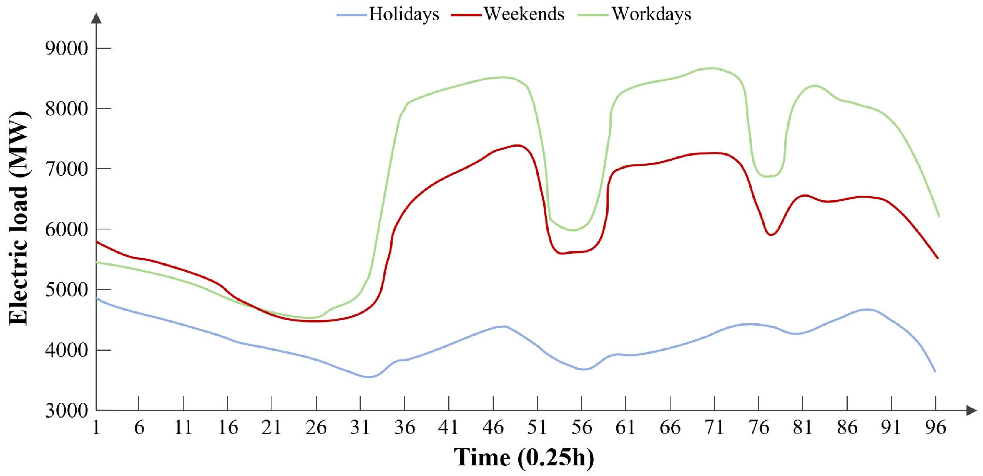
As shown in Figure 8, the weekday curve peaks during the morning hours, experiences a decline in load during the midday break, peaks again in the afternoon working hours, declines during the dinner time, reaches the last small peak of the day at night, and then gradually descends into late night. In contrast to the weekday load, the weekend load shows an overall decrease in value. The variation trend of the load on public holidays significantly differs from the trends of the aforementioned two types of loads.

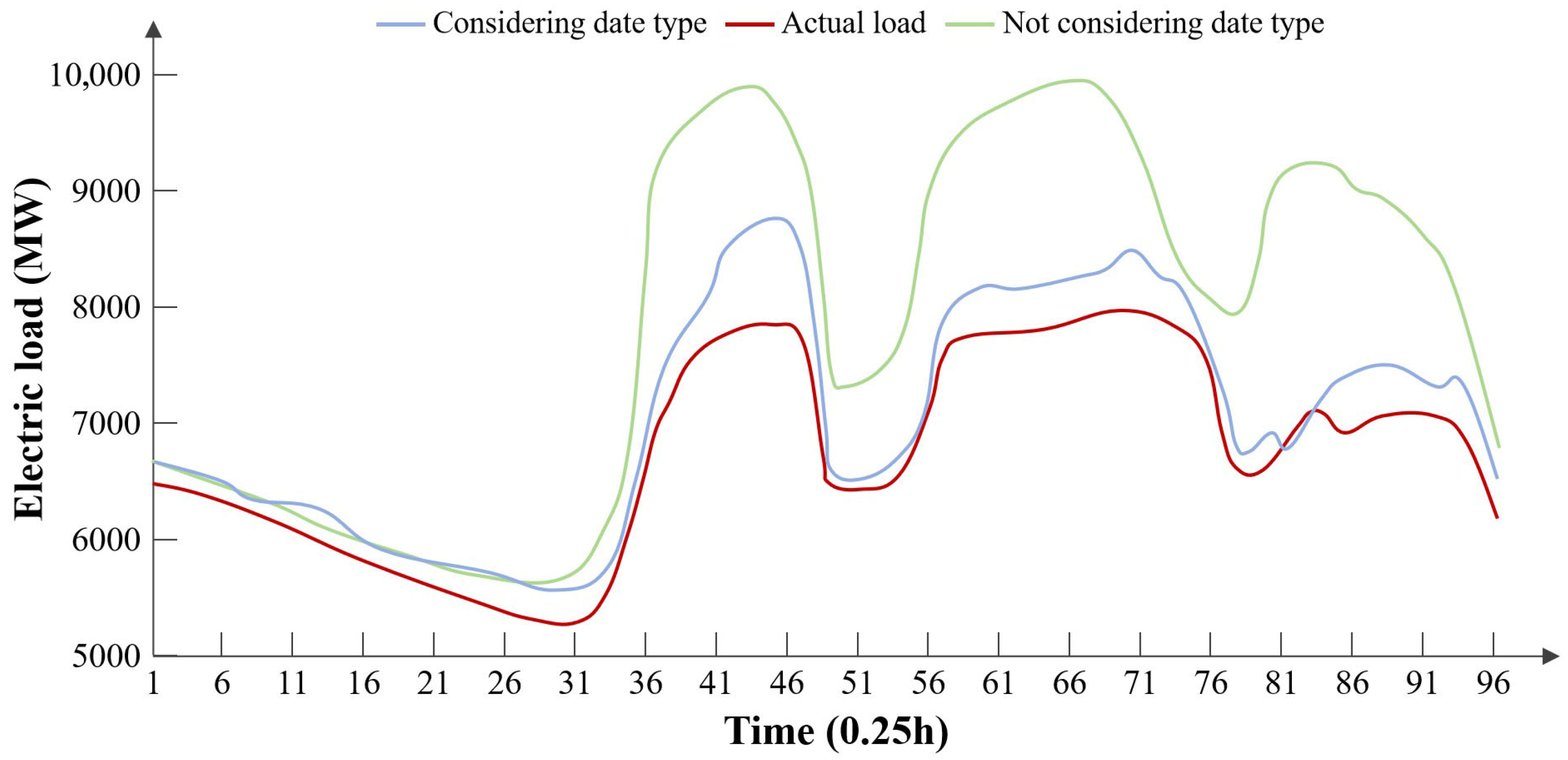
Therefore, we created a new feature called ‘date type’ to account for holiday factors in the neural network, where weekdays are represented by 1, weekends by 2, and public holidays by 3. We used GRU models that consider and do not consider date types to predict weekend loads, as shown in

Table 6. Comparison of prediction errors for weekend days.

Comparative Experiments	MAPE	MAE	RMSE
Considering date types	3.369%	218.185	249.298
Not considering date types	15.421%	1055.649	1276.668

and Figure 9.

From the experimental results, it can be seen that the power load prediction model that does not consider date types performs poorly in predicting weekend loads. In contrast, the power load prediction model that takes date types into account is able to accurately grasp the key information that ‘some businesses rest on weekends’, thereby achieving higher accuracy.

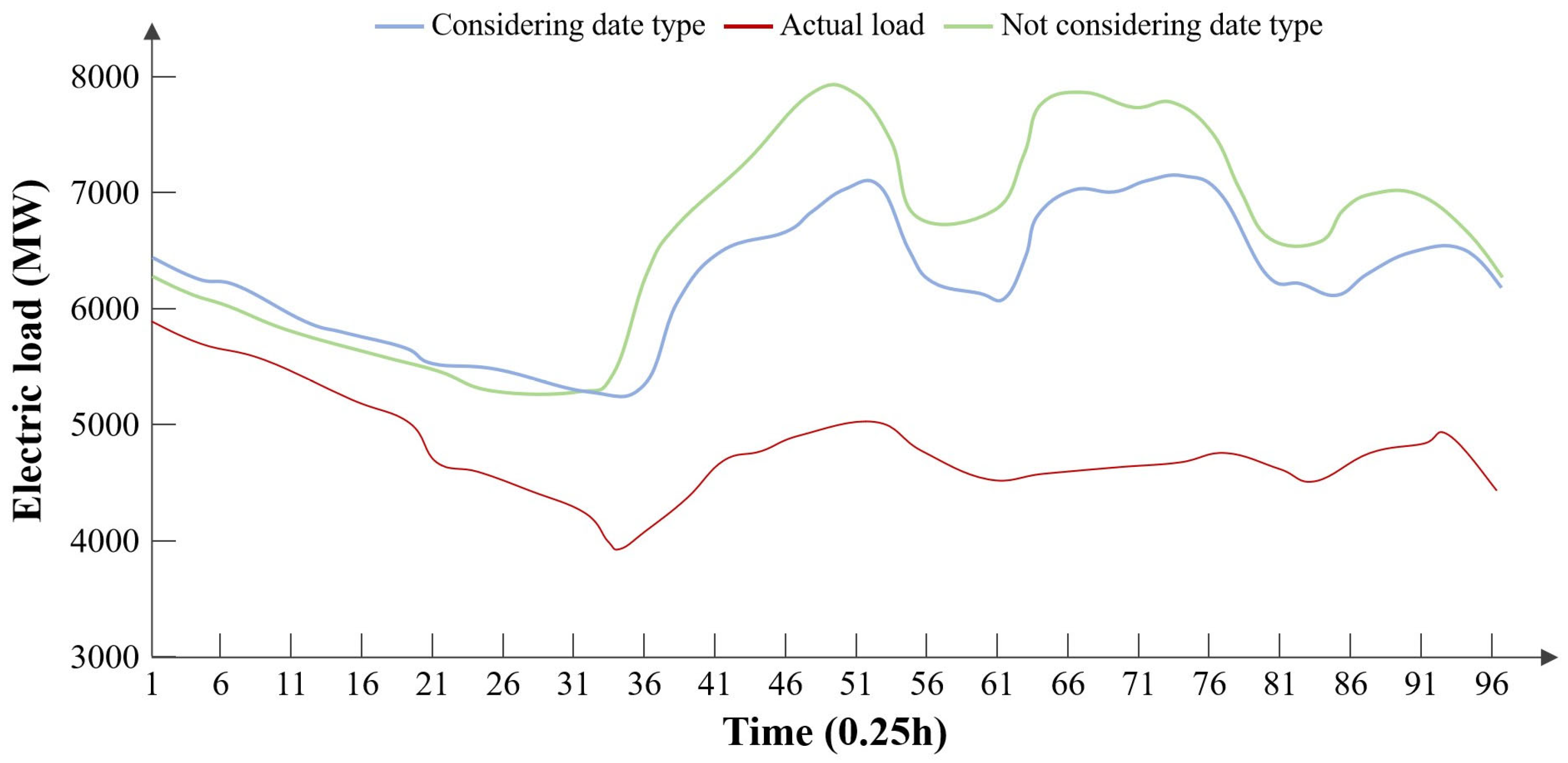
However, when the date type of the prediction day is 3, the model exhibits significant overfitting, as shown in Figure 10. Although the model that considers date types is superior to the one that does not, the overall accuracy remains low and fails to meet the requirements for power load forecasting. The main reason for this phenomenon is that there are too few recent training samples from statutory holidays for the prediction day. For example, when predicting the load for a certain holiday, only one holiday sample is included among the 57 training samples. If an attempt is made to increase the number of statutory holiday samples by expanding the training set with older historical data, then the model’s accuracy may be compromised due to interference from the distant historical data. Therefore, even with the consideration of date types, the model does not achieve sufficient accuracy.

3. Electricity Load Forecasting Method Based on BP-GRU Model

3.1. Selection of Weight Parameter Optimization Algorithm

The parameter optimization algorithm is a core component of training deep learning models. It determines how the neural network learns, which directly impacts the effectiveness of the learning process. Generally speaking, the parameter optimization algorithm optimizes parameters such as the weights of the neural network using a large set of sample data, once the structure of the neural network has been finalized. This section examines several typical parameter optimization algorithms and compares their characteristics when applied to the GRU model. Ultimately, we select the algorithm with the lowest testing error to apply in the method proposed in this chapter. Common parameter optimization algorithms include:

Gradient Descent (GD): Gradient descent is one of the most classic methods for training neural networks. Its fundamental idea is to adjust parameters in the direction where the gradient decreases the fastest, thereby reducing the loss.

Momentum: The Momentum algorithm was developed to address the instability and tendency to become trapped in local minima that can occur with gradient descent. It simulates the inertia of a moving object by giving the optimization process momentum. This allows the updates to retain some historical direction while also considering the current gradient, collectively determining the final update direction. This approach effectively helps prevent getting stuck in local optima.

NAG (Nesterov Accelerated Gradient): NAG improves upon the Momentum method and converges more quickly. The principle is to compute the gradient one step ahead along the direction of the momentum term and combine it with the current gradient to determine the upcoming gradient value for the update.

AdaGrad (Adaptive Gradient Algorithm): AdaGrad is an adaptive learning rate gradient descent algorithm that decays the learning rate throughout the training iterations. Parameters that are updated frequently have their learning rates reduced more quickly, allowing them to move in directions closer to the bottom of the loss curve, thus accelerating convergence.

Adadelta (Adaptive Delta): Adadelta is an extension of the AdaGrad algorithm that does not rely on a global learning rate.

RMSProp (Root Mean Square Propagation): This algorithm is an improvement over AdaGrad and effectively reduces the risk of “gradient explosion,” thereby avoiding the problem of a rapidly decaying learning rate.

Adam (Adaptive Moment Estimation): Adam stands for Adaptive Moment Estimation. It combines ideas from both the Momentum and RMSProp algorithms, using first and second moment estimates of the gradients to dynamically adjust the learning rate for each parameter.

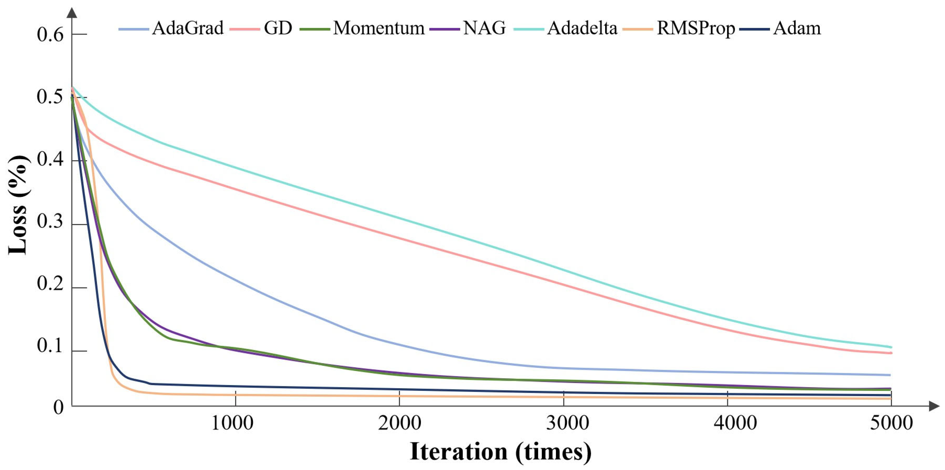
Apply the above seven parameter optimization algorithms to the GRU neural network and conduct comparative experiments on the test set. The results of the comparison experiment regarding the decrease in loss function are shown in Figure 11. From the figure, it can be seen that the Adadelta algorithm and the DG algorithm are significantly lagging behind other algorithms both in terms of convergence rate and convergence limit. In contrast, the RMSProp algorithm and the Adam algorithm achieve lower loss values and converge at a noticeably faster rate than the other algorithms.

We will compare the error results from the validation set experiments, as shown in

Table 7. Comparison Table of Error Metrics for Common Parameter Optimization Algorithms.

Algorithm Name	MAPE	MAE	RMSE
AdaGrad	1.378%	106.186	126.948
GD	1.928%	149.888	177.619
momentum	1.302%	112.482	168.897
NAG	1.558%	120.233	138.571
Adadelta	1.379%	113.390	147.517
RMSProp	1.159%	97.582	127.621
Adam	1.601%	136.508	164.311

. The results indicate that the neural network model using the RMSProp algorithm has a slightly lower error compared to the neural network model using the Adam algorithm. Therefore, this chapter adopts the RMSProp optimization algorithm for parameter optimization.

3.2. Construction of GRU and BP Neural Network Models

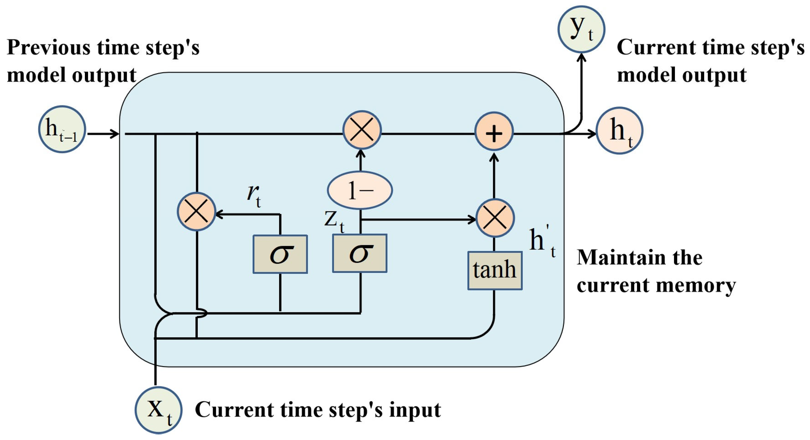
The GRU neural network is an improved version of the LSTM neural network. It reduces some parameters based on the LSTM model, making the model easier to converge during training. Therefore, the GRU neural network is more suitable for handling situations with fewer data samples, as it is less likely to overfit. The structure diagram of the GRU is shown in Figure 12. The principles of GRU are similar to those of LSTM, as both use gating mechanisms to control input, including the reset gate and the update gate.

The reset gate determines whether the current state should be combined with historical information, as expressed in Equation (1):

$$r_t=\sigma \left(W^{(r)}{x}_t+U^{(r)}{h}_{t-1}\right),$$

(1)

where $x_i$ is the input at time t, $h_{t-1}$ is the output from the previous time step, $\sigma$ is the sigmoid activation function, and $W_r$ and $U_r$ are parameters that need to be adjusted during the training phase. The update gate determines how much of the previous state is retained in the current time step, as expressed in Equation (2):

$$z_t=\sigma \left(W^{(z)}{x}_t+U^{(z)}{h}_{t-1}\right),$$

(2)

where $W_z$ and $U_z$ are parameters that need to be optimized during the training process. Regarding the current memory content, the GRU cell represents the memory retained at the current time step t as $h_t^{\prime }$:

$$h_t^{\prime }=\tanh \left(r_1\ast U{h}_{t-1}+W{x}_t\right).$$

(3)

Here $*$ denotes matrix multiplication, and U and W are the training parameters for the memory retrieval process. The final memory at the current time step is the retained historical memory plus the current state, which is then output to the cell at time t + 1:

$$h_t=\left(1-z_t\right)\ast h_t^{\prime }+z_t\ast h_{t-1}.$$

(4)

We constructed a GRU neural network and determined a set of hyperparameters usable for the experiments through experiments. The results of the hyperparameter experiments are shown in

Table 8. Comparison of hyperparameter experimental results.

Time Step Size	Number of Feature Cycles	Learning Rate	Number of Hidden Layers	Batch Size	Training Set Size	MAPE
1	2	0.0006	3	96	56	1.527%
1	3	0.0006	3	96	56	1.389%
1	3	0.0006	4	96	56	2.259%
1	3	0.0006	2	96	56	2.164%
1	3	0.0006	3	96	36	2.129%
1	3	0.0006	3	96	76	1.590%
1	4	0.0006	3	96	56	2.469%
1	3	0.0006	3	48	56	2.782%
1	3	0.0006	3	120	56	2.521%
1	3	0.001	3	96	56	2.101%
15	3	0.0006	3	96	56	1.503%
30	3	0.0006	3	96	56	1.886%
5	3	0.0006	3	96	56	1.146%
5	3	0.0006	3	20	56	2.868%
5	3	0.0006	3	36	56	1.911%

. The hyperparameters include the number of hidden layer units, the number of cycles of input features, the learning rate, the number of hidden layers, batch size, and the size of the training set. The number of cycles of input features indicates how many cycles of feature data are input during the experiment. Since the variation in power load data is periodic, fully considering the feature data at historical interval time points aids the neural network in predicting power loads. However, taking into account too distant historical cycle data will reduce the quality of training; therefore, we included this hyperparameter in the tuning range. Similarly, the size of the training set refers to the number of historical data samples in the training set. In power load prediction research, there is a strict temporal relationship between the test set and the training set. The training set must consist of recent historical data relative to the test set and should not be spaced too far apart from the test set data. Therefore, the selection of the training data size will also affect the model’s prediction accuracy.

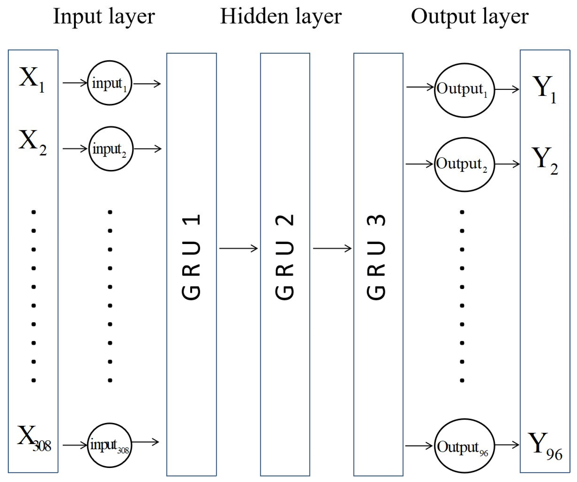
We selected the combination of hyperparameters that yielded the lowest error metric, MAPE, to construct the GRU neural network. The GRU model architecture comprises five layers: an input layer, three hidden layers, and an output layer. The model employs the RMSProp optimizer and uses Mean Absolute Error (MAE) as the loss function. The structure of the GRU neural network is shown in Figure 13, with input features including meteorological data from the past three days, date type, and all-day load values, as well as the meteorological features and date type for the predicted day. The output is the power load values for the next 96 time points.

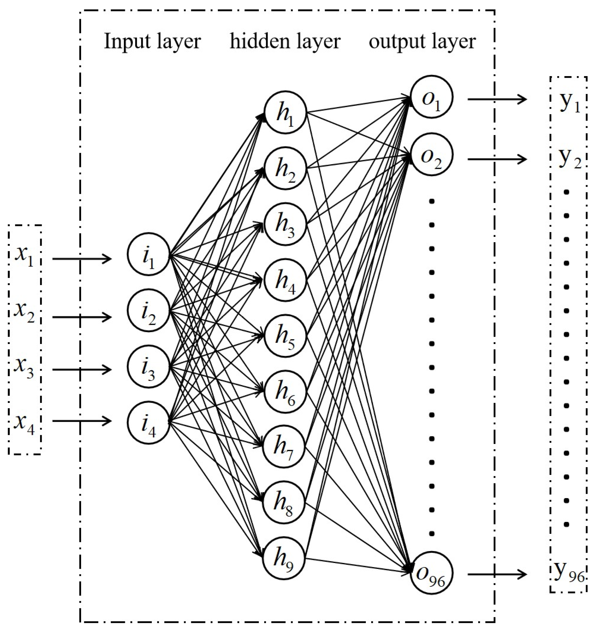
In order to enable the prediction model to learn from a training set composed solely of isolated holiday data, we used a BP neural network specifically to predict power load on holidays. The structure of the BP neural network we constructed is shown in Figure 14, where the inputs are the maximum temperature, minimum temperature, average temperature of day i, and the last moment power load value from the previous i − 1 days, totaling four dimensions of input. The model employs the RMSProp optimizer and uses MAE as the loss function. The output consists of the power load values at 96 points for that day, resulting in a total of 96 dimensions of output.

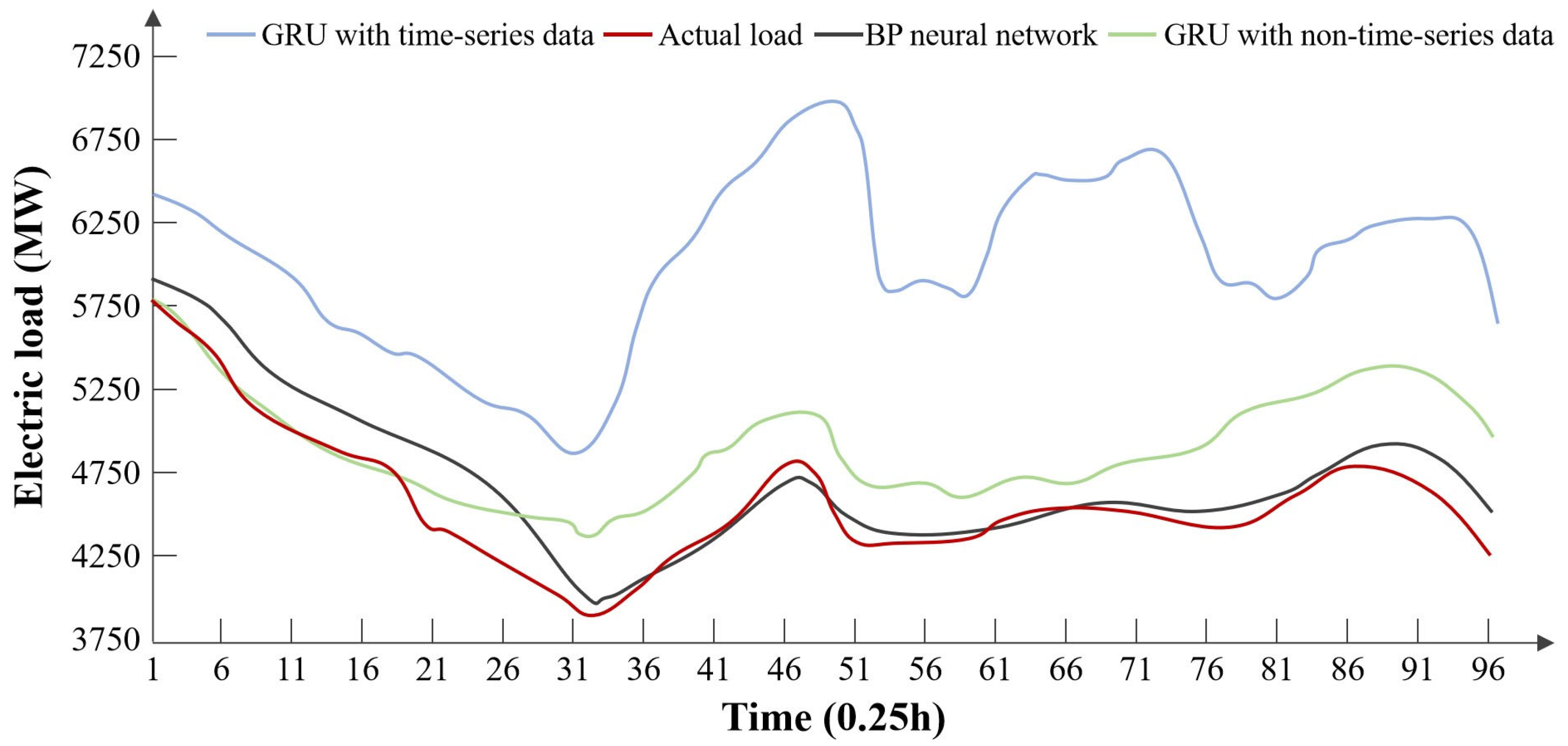
The comparison results of the methods are shown in Figure 15 and

Table 9. Table of forecasting error results for holiday electricity loads.

Comparison Experiment	MAPE	MAE	RMSE
GRU for processing time series data	34.518%	1527.302	1647.454
BP	2.643%	122.010	154.090
GRU for handling non-time series data	6.089%	265.153	309.753

. In the experiments using the GRU neural network to predict power loads on statutory holidays with time series data, although the data has a temporal nature, the samples for statutory holidays are sparse within the sequentially ordered data, leading to larger errors at this point [19,20,21]. Therefore, we created an independent training set composed solely of all statutory holiday sample data; the data in this training set is temporally isolated from each other, with weak connections and varying time intervals, making it non-temporal data that is difficult for recurrent neural networks to handle. From the results, it can be concluded that the BP neural network effectively mitigated the overfitting phenomenon of the GRU model. When processing these non-temporal data, the GRU neural network futilely considers the temporal relationships within the data, resulting in decreased accuracy. Thus, in this section, we chose the BP neural network to specifically predict power loads on holidays.

3.3. Prediction Process of BP-GRU Model

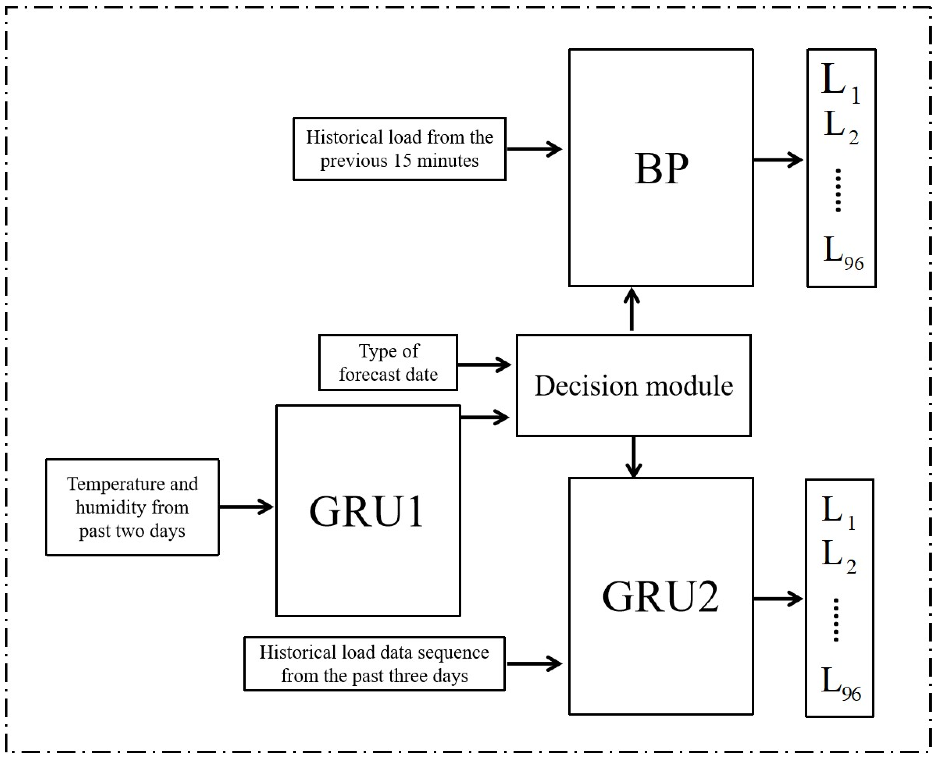
If we rely solely on the GRU model, its inherent time-series processing mechanism—while beneficial for regular load forecasting—proves disadvantageous for holiday load prediction. In contrast, the BP neural network lacks this sequential dependency mechanism, making it better suited for standalone holiday load forecasting but less effective for non-holiday scenarios. Given these complementary strengths and weaknesses, we integrated both approaches. Based on the above experimental research, this chapter proposes a short-term electricity load forecasting method that combines the BP neural network and the GRU neural network. The method’s structural diagram is shown in Figure 16. Among them, GRU1 is specifically designed for predicting meteorological data. Since future meteorological data cannot be measured at the current time when performing short-term electricity load forecasting, our proposed method first predicts the meteorological data for the next day using the GRU1 module. The predicted data is then input into the judgment module along with historical meteorological data.

The judgment module has two functions. First, it determines whether to use the GRU model or the BP model based on the type of predicted day. When the predicted day type is “1”: a legal holiday, the judgment module will use the BP neural network model. In contrast, when the predicted day types are “2” or “3”: working days or weekend holidays, the judgment module will use the GRU model and output the predicted day type to GRU2. Then, based on the human comfort level ET discriminant, it decides whether to use temperature factors.

$$ET=T_d-0.55\left(1-r\right)\left(58-T_r\right)$$

(5)

Among them, $T_d$ represents the highest temperature of day T, and r is the relative humidity corresponding to the highest temperature. When ET is less than or equal to 18.9 degrees Celsius, it indicates discomfort in the human body caused by excessive cold; whereas when ET is greater than 25.6 degrees Celsius, it indicates discomfort caused by excessive heat. When ET falls within the “discomfort” range, the model determines that it is necessary to consider temperature-sensitive loads and inputs all temperature data into the neural network model; otherwise, the model will conclude that temperature data is not needed at that time and will input 0 into the neural network model.

The BP neural network model is used to predict during legal holidays, with the historical load value from the previous 15 min being one of the input features, serving as a reference benchmark for the model’s predictions. GRU2 is a neural network model used to predict electricity load, with input features including historical load data from the past three days, historical temperature data from the past three days, date type data from the past three days, predicted day type data, and predicted day temperature data.

The flow of the judgment module is as follows:

Step 1: Receive the temperature forecast for day i and store the historical temperature data from the previous three days as variable $T_i$, along with humidity forecast Ri and predicted day type data $P_i$.

Step 2: Calculate human comfort level ${ET}_i$ for day i and determine if the sensation of comfort for humans on day i is acceptable. If yes, proceed to Step 3; otherwise, proceed to Step 4.

Step 3: Modify variable content, Output = {0}.

Step 4: Modify variable content, Output = {$T_i$}.

Step 5: Determine if the date type is a legal holiday. If yes, proceed to Step 6; if no, proceed to Step 7.

Step 6: Output variable Output to the BP model and proceed to Step 8.

Step 7: Modify variable content Output = {$T_i$, $P_i$}, output variable Output to GRU2, and proceed to Step 8.

Step 8: End.

4. Validation and Analysis of the Proposed Method

This paper compares the proposed BP-GRU method with traditional forecasting models across four typical days. The results are presented in Figure 17, Figure 18, Figure 19 and Figure 20, and the error metrics are summarized in

Table 10. Comparison of Model Errors for Typical Day 1. The LSTM model is derived from reference [6]; the GRU model is based on reference [14]; the BP model comes from reference [7]; and the RNN model is sourced from reference [9].

Model Name	MAPE	MAE	RMSE
BP-GRU	1.675%	99.425	127.564
GRU	1.904%	107.554	127.814
LSTM	2.627%	153.572	177.899
BP	5.938%	356.058	386.717
RNN	2.742%	152.840	201.621

,

Table 11. Comparison of Model Errors for Typical Day 2. The LSTM model is derived from reference [6]; the GRU model is based on reference [14]; the BP model comes from reference [7]; and the RNN model is sourced from reference [9].

Model Name	MAPE	MAE	RMSE
BP-GRU	1.661%	144.361	205.116
GRU	2.139%	171.527	199.845
LSTM	2.487%	189.120	206.682
BP	4.452%	343.578	401.930
RNN	3.561%	260.895	338.682

,

Table 12. Comparison of Model Errors for Typical Day 3. The LSTM model is derived from reference [6]; the GRU model is based on reference [14]; the BP model comes from reference [7]; and the RNN model is sourced from reference [9].

Model Name	MAPE	MAE	RMSE
BP-GRU	1.454%	115.092	183.382
GRU	2.161%	168.063	224.612
LSTM	2.173%	164.251	209.053
BP	3.313%	202.724	243.532
RNN	3.462%	207.067	263.706

and

Table 13. Comparison of Model Errors for Typical Day 4. The LSTM model is derived from reference [6]; the GRU model is based on reference [14]; the BP model comes from reference [7]; and the RNN model is sourced from reference [9].

Model Name	MAPE	MAE	RMSE
BP-GRU	1.398%	48.027	55.941
GRU	8.027%	286.726	319.844
LSTM	14.414%	531.438	626.879
BP	1.499%	53.695	64.032
RNN	14.236%	218.561	302.697

.

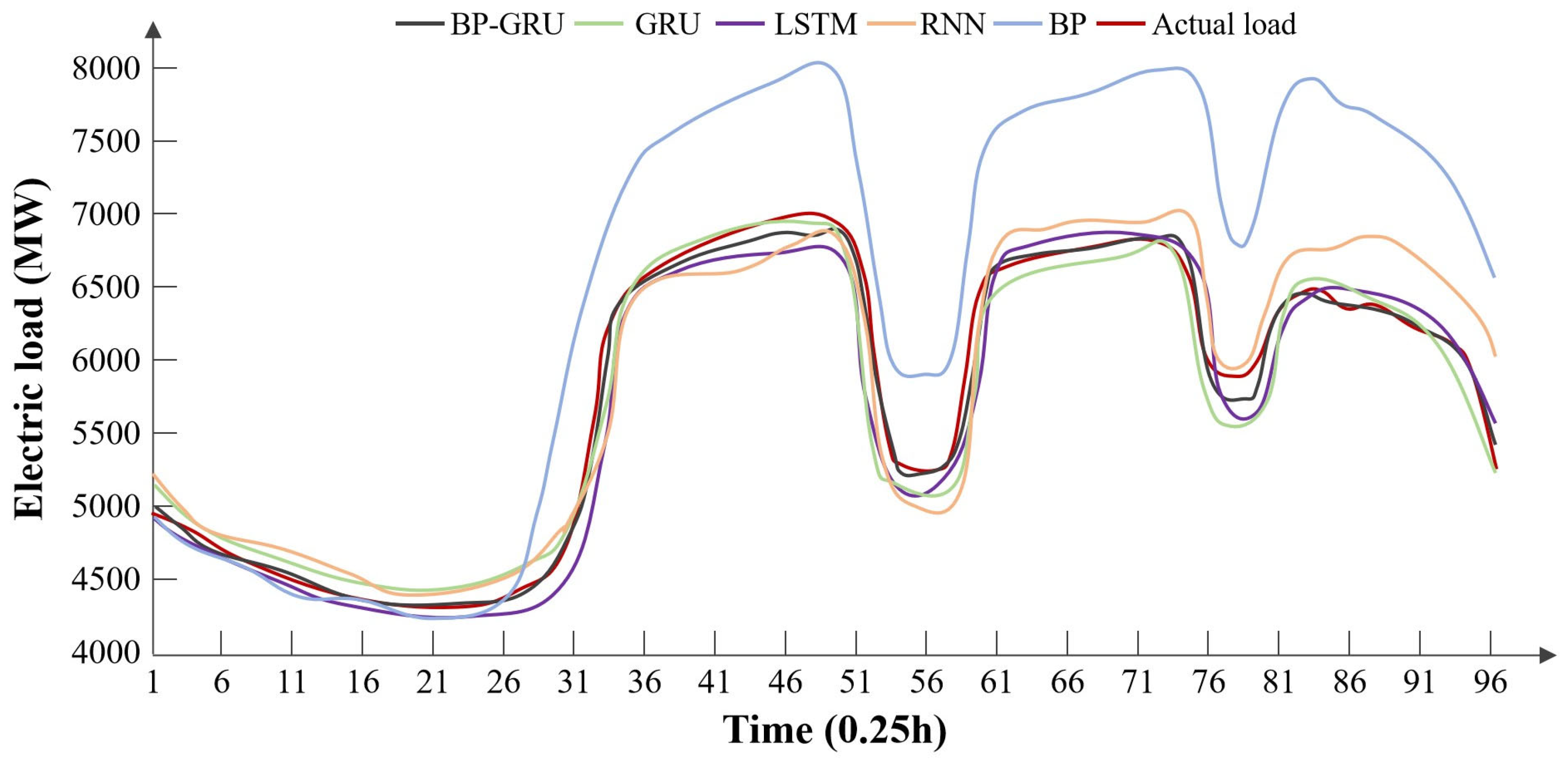
From the prediction results for Typical Day 1, it can be observed that the load change trends predicted by the models involved in the comparison are generally consistent. The BP-GRU model and the standard GRU model show similar performance. However, there are differences in the magnitude of the changes, with the BP neural network model exhibiting a larger deviation. We speculate that this may be due to the fact that, in the test set for Typical Day 1, the BP neural network’s inability to leverage the temporal trends in the time series data is amplified.

According to the error metrics, the BP-GRU has the lowest error. The advantage of this model over the traditional GRU model is its ability to account for human comfort levels, thereby mitigating the negative impacts of temperature factors, resulting in higher accuracy.

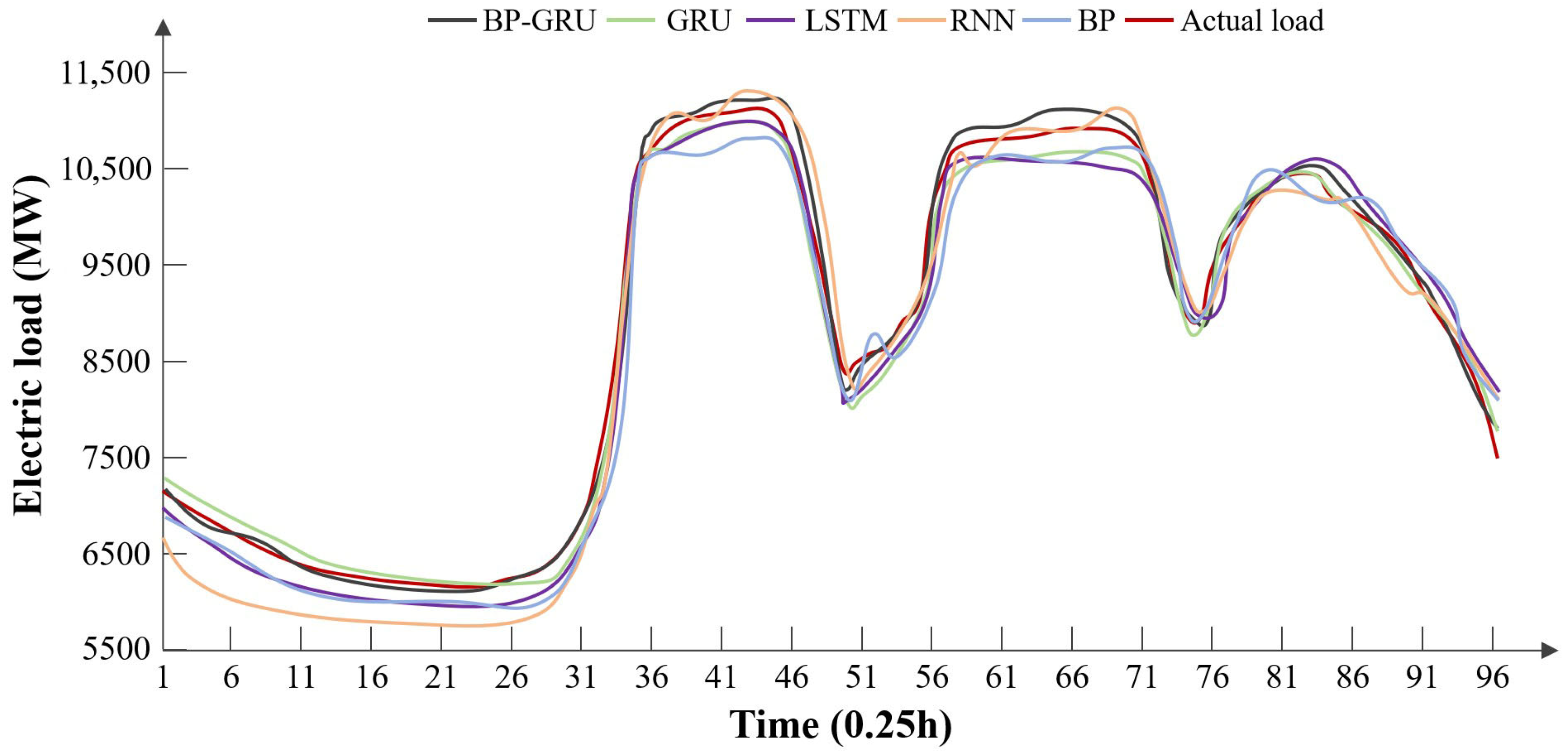
From the prediction results for Typical Day 2, it can be seen that all five models involved in the comparison have effectively captured the electricity load trends for the upcoming day. The BP-GRU model aligns closely with the standard values, while the other models show varying degrees of fluctuation and deviation.

From the error table, we can conclude that the BP-GRU model and the GRU model have lower errors, benefiting from their ability to handle small sample data, thus outperforming other recurrent neural networks. In contrast, the BP neural network has the highest error due to its lack of capability in processing time series data.

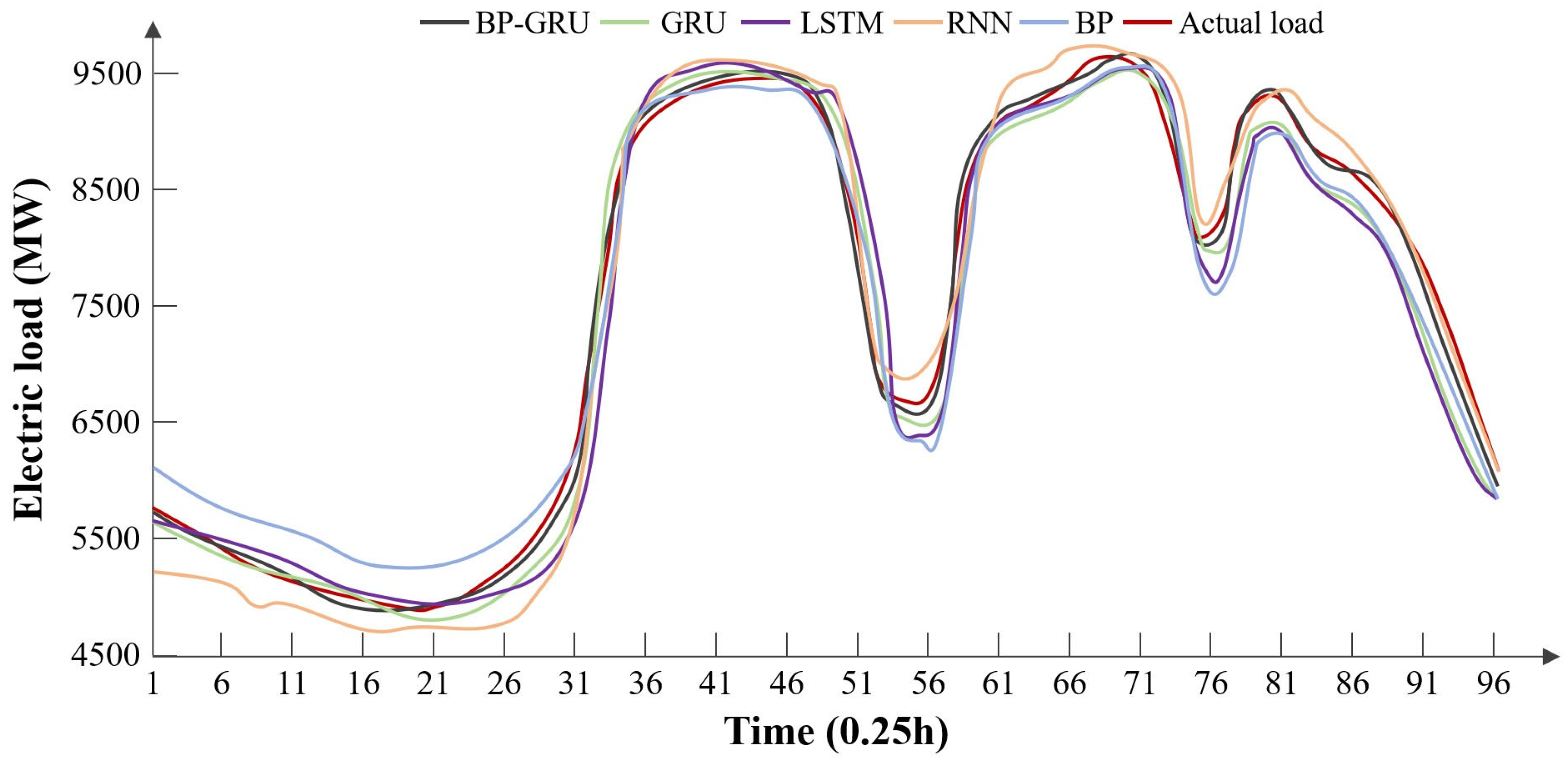
From the results of Typical Day 3, it is evident that the RNN model and the BP neural network model exhibit significant deviations at time points 1 to 31 but yield better predictions overall between time points 31 and 71. The curves of the BP-GRU model, GRU model, and LSTM model show relatively minor differences overall.

According to the error metrics, the BP-GRU model has the lowest error. On Typical Day 3, human comfort levels were relatively high, without temperature-sensitive loads; therefore, the BP-GRU model did not utilize temperature factors, avoiding the negative impacts associated with temperature and achieving higher accuracy.

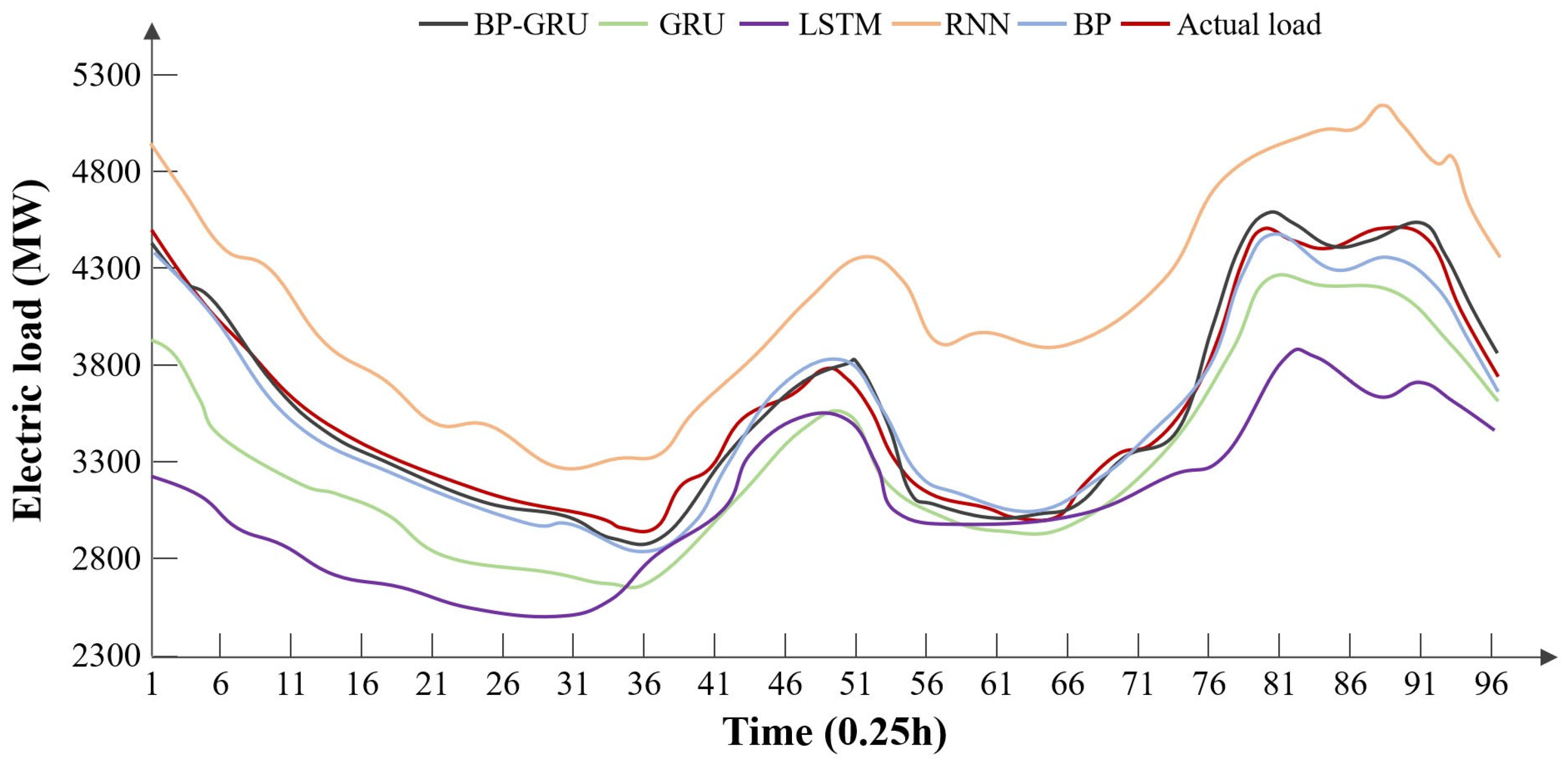
From the prediction results for Typical Day 4, it is noted that the prediction day falls during the New Year holiday, resulting in larger errors for the recurrent neural network models when processing non-temporal datasets. However, the BP-GRU model can leverage the branch method of the BP neural network model during statutory holidays, allowing it to better handle these non-temporal data.

The error results indicate that the RNN, LSTM, and GRU models have relatively large errors. This is because these types of neural networks tend to overemphasize the temporal relationships between samples during training, whereas the data samples in the statutory holiday training set are isolated from each other, with minimal mutual influence and varying time intervals, thus representing non-temporal data. The BP neural network, however, is capable of handling such data, which is why both the BP-GRU model and the BP neural network model can achieve lower errors.

In addition to the test analysis of the four typical days mentioned above, we conducted supplementary tests using power load data from 20 different dates. The test results are presented in

Table 14. Statistical table of supplementary test results for the proposed method.

Test Group	MAPE	Test Group	MAPE
Day 1 (Spring workdays)	1.271%	Day 11 (Autumn workdays)	1.409%
Day 2 (Spring workdays)	1.183%	Day 12 (Autumn workdays)	1.732%
Day 3 (Spring workdays)	0.923%	Day 13 (Autumn holidays)	0.971%
Day 4 (Spring holidays)	1.785%	Day 14 (Autumn holidays)	1.285%
Day 5 (Spring holidays)	1.052%	Day 15 (Autumn holidays)	1.555%
Day 6 (Summer workdays)	1.342%	Day 16 (Winter workdays)	1.912%
Day 7 (Summer workdays)	1.871%	Day 17 (Winter workdays)	1.234%
Day 8 (Summer workdays)	0.842%	Day 18 (Winter holidays)	1.567%
Day 9 (Summer workdays)	1.623%	Day 19 (Winter holidays)	1.124%
Day 10 (Summer holidays)	1.198%	Day 20 (Winter holidays)	1.663%

. Among these test dates, both workdays and holidays across different seasons are covered. During spring and autumn, the power load exhibits a low proportion of temperature-sensitive demand. In these seasons, the model does not need to consider temperature factors when determining the forecasted load based on the human thermal comfort calculation model. In contrast, during summer and winter, the power load is characterized by a high proportion of temperature-sensitive demand, with overall electricity consumption reaching peak levels. Under these conditions, the model must account for temperature factors when determining the forecasted load using the human thermal comfort calculation model. Experimental results indicate that the proposed method achieves errors consistently below 2%, thereby validating its effectiveness.

5. Conclusions

This paper conducts research on short-term electricity load forecasting methods based on multi-factor analysis and the BP-GRU model, primarily addressing the issue of low accuracy encountered by traditional time series forecasting models when predicting electricity loads during holidays. The main findings are summarized as follows:

Several influencing factors such as temperature, humidity, rainfall, and type of date were analyzed. It was found that temperature impacts load forecasting differently across seasons; it has a positive effect in summer and winter, while negatively affecting forecasts in spring and autumn. Humidity and rainfall showed a low correlation with load and were therefore not considered. The type of date has a significant impact on load forecasting. The analysis indicates that both temperature and date type are important factors to consider.

This study proposes a BP-GRU combined model that utilizes the strengths of the GRU model in handling time series data and the feasibility of the BP model for non-time series data. This model flexibly processes holiday load forecasts by treating them as non-temporal data, thereby avoiding interference from recent historical data during holidays. Additionally, the model effectively leverages the positive influence of temperature on load forecasting according to human comfort level models.

Compared to existing load forecasting models, the proposed model excels in predicting electricity loads during holidays. In tests conducted on four typical days, the Mean Absolute Percentage Error (MAPE) values were 1.675%, 1.661%, 1.454%, and 1.398%; the Mean Absolute Error (MAE) values were 99.425, 144.361, 115.092, and 48.027; and the Root Mean Square Error (RMSE) values were 127.564, 205.116, 183.382, and 55.941. All error metrics for the proposed model are lower than those of existing models, particularly demonstrating significant advantages in forecasting electricity loads on holidays.