Uncertainty-Based System Flexibility Evaluation and Multi-Objective Collaborative Optimization of Integrated Energy System

Abstract

With the advancement of integrated energy systems (IES) and the increasing penetration of variable renewable energy, IES confronts complex uncertainties that necessitate enhanced flexibility. Therefore, this study focuses on improving IES flexibility. To this end, multi-dimensional flexibility evaluation indexes for the “Source–Structure–Demand” dimensions were established, and a multi-objective optimization model considering flexibility and source–demand side uncertainties was developed. The flexibility evaluation indexes include the Grid Dependency Level (GDL) for the source side, Insufficient Flexible Resource Probability (IFRP) for the structure side, and Loss of Load Probability (LOLP) for the demand side. Moreover, considering the distinct adjustment response times and inertia of different energy flows during IES operation, thermal and electrical energy are optimized on separate time scales. Thus, the multi-objective optimization constitutes a multi-time scale, high-dimensional, non-convex nonlinear model targeting economy, flexibility, security, and low carbon emissions. This paper employs single-economy objective, single-flexibility objective, and multi-objective optimization to analyze IES configuration, operation, risk, carbon emissions, and flexibility. The results indicate that poor flexibility leads to high operational risk, while excessive pursuit of flexibility incurs high costs and destabilizes operations. By implementing this multi-objective optimization, IES flexibility is enhanced while ensuring system economic performance. It also addresses the flexibility deficiency in traditional single-economy objective optimizations. Additionally, the system increases the renewable energy absorption rate by approximately 10%.

1. Introduction

Energy is critical to national economic and social development. Constructing clean, efficient, and low-carbon energy systems while promoting energy transition has become pivotal for achieving harmonious economic–environmental development globally. In this context, the integrated energy system (IES) has emerged as a key trend in the global energy landscape [1,2,3,4]. With the development of IES, its structure becomes increasingly complex, energy demand grows more dynamic, and the inherent intermittency, randomness, and volatility of renewable energy (e.g., wind and solar power) subject the system to complex source–demand uncertainties. This introduces challenges and risks to fluctuation response, supply–demand balance, stable operation, and collaborative optimization of IES.

With rising renewable energy penetration, IES is characterized by high uncertainty, strong randomness, and low inertia, imposing stricter requirements on system flexibility. Flexibility is fundamental to system safety, stability, reliability, and its ability to mitigate fluctuations. Thus, enhancing system flexibility to ensure supply–demand balance and enable efficient renewable energy consumption under complex source–demand uncertainties represents a core focus of IES research

Flexibility research has advanced across diverse fields, including manufacturing [5,6,7,8], construction [9,10,11,12,13], transportation [14,15,16,17], energy and power [18,19,20,21] and the hydrogen industry [22,23,24]. Flexibility is commonly defined as a system’s adaptability to fluctuating conditions, though its interpretation varies significantly across applications. Numerous studies have explored flexibility in energy and power sectors, but definitions and evaluation methods differ based on specific application aspects [25,26], primarily focusing on the “Generation–Distribution–Storage” chain of grids and electrical systems. For instance, local flexibility markets and trading mechanisms for grid distribution system operators have been extensively studied [27]. However, due to multi-energy flow coupling and terminal application characteristics, IES flexibility research diverges notably from traditional grid power systems, and current IES flexibility studies remain insufficient.

The core of flexibility research lies in its evaluation. In current flexibility studies within the energy and power industry, evaluation indexes are mostly system-specific and exhibit diverse forms. In [28], insufficient ramping resource expectation (IRRE) based on the loss of load expectation (LOLE) was established to evaluate electric system flexibility, but aimed at the electric power supply regulation capacity of the grid structure. Thatte et al. [29] adopted a similar metric, Loss of Ramping Probability (LORP), as a flexibility index for electric grids. Beyond ramping resource evaluations, Ulbig and Anderson [30] incorporated power supply capacity, ramping resources, and ramping duration to comprehensively assess power system flexibility from the adjustment supply side. Additionally, the ratio of the feasible operation region to the constraint region has been used to characterize system flexibility levels [31]. Most of the existing flexibility evaluation indexes are based on the indexes in the above studies, yet they primarily focus on electrical systems and overlook IES flexibility assessment. Perera et al. [32] attempted to define the evaluation indexes and established six indexes comprehensively: NPV, waste of renewable energy, loss of load probability, grid integration level, net interactions and fuel consumption of the generator. In [33], off-peak residual renewable energy transfer rate and off-peak grid transfer rate were used to evaluate the flexibility of IES, but focused on residential buildings rather than on a complete energy system.

The overview of the literatures shows current flexibility research and evaluation largely focus on the grid, emphasizing its renewable energy absorption potential. For IES, flexibility evaluation and research remain insufficient. Existing studies mainly assess whether system energy supply and demand can balance under fluctuations due to increased renewable energy penetration. While flexibility exhibits multiple characteristics, existing evaluation indexes do not fully consider these traits or each dimension of IES, failing to form logical relationships. Moreover, amid multiple uncertainties, IES faces heightened volatility, making sufficient flexibility critical for stable operation. Current flexibility assessment methods often rely on deterministic scenarios, failing to capture inherent uncertainties in modern IES, such as renewable energy variability and demand fluctuations. Thus, integrating both uncertainty and flexibility in IES collaborative optimization is essential, as this enhances operational robustness and provides a more comprehensive decision-making basis in dynamic environments. However, existing flexibility evaluation indexes cannot effectively integrate uncertainties, hindering their ability to meet the high-uncertainty, high-randomness flexibility requirements of modern IES.

Several studies have acknowledged the importance of IES uncertainty and flexibility, attempting to optimize IES while considering these factors. Turk et al. [34] and Dini et al. [35] employ stochastic programming to model renewable energy uncertainties, aiming to enhance IES economic and flexible operation. In [36], a two-stage robust optimization dispatch model of the power system considering flexible supply and requirement is developed. However, these studies transferred flexibility to economic cost or equipment capacities and focused on flexibility analysis rather than on taking this as an optimization objective. In the actual application of IES, the system faces more complex situations where multiple uncertainties exist and may lead to a decrease in the IES performance, while higher flexibility will enable the system to withstand uncertainties for a long time. Taking flexibility as the goal of system optimization can fundamentally improve the level of system flexibility.

Therefore, to better address uncertainty-induced random disturbances, improve renewable energy utilization, and enhance IES operational flexibility, this paper establishes a multidimensional IES flexibility evaluation index system and a multi-objective optimization model considering source–demand side uncertainties and flexibility. The contributions of this paper include the following:

(1)

Multi-dimensional Flexibility Evaluation System: This paper establishes a novel flexibility evaluation framework for IES across ‘Source–Structure–Demand’ dimensions, addressing gaps in existing research on flexibility evaluation metrics under uncertainty and providing a universal tool for IES flexibility analysis.

(2)

Multi-objective Optimization Model: A multi-objective optimization model is developed, integrating economy, flexibility, low-carbon performance, and risk management. This approach enhances system flexibility and overall performance under uncertainty, surpassing traditional single-objective methods and offering a more comprehensive solution for the optimal operation of IES.

(3)

Enhanced Uncertainty Handling Capability in a Low-carbon Context: The model improves the system’s ability to handle uncertainties while boosting renewable energy integration, aligning with global low-carbon goals and offering practical solutions for sustainable energy systems.

These innovations provide a systematic and holistic approach to IES flexibility and optimization, contributing valuable insights for future research and applications.

The remainder of this paper is organized as follows: Section 2 presents the overall description of IES flexibility and its evaluation index and Section 3 presents the detailed multi-objective optimization model. Section 4 provides the case study details, and the results are reported and discussed in Section 5. Finally, Section 6 concludes the study.

2. System Flexibility and Its Evaluation Index

In this section, the details of a generic IES are first defined. Subsequently, IES flexibility and its evaluation index, along with the multi-objective optimization framework considering flexibility and uncertainty, are presented in detail.

2.1. A Generic Integrated Energy System

To increase the relevance of the proposed flexibility evaluation, this study adopted a typical grid-connected IES, whose structure can be seen in many existing studies. The methods and findings of this study can be applied to energy systems for large public buildings, residential/industrial areas, and urban cities.

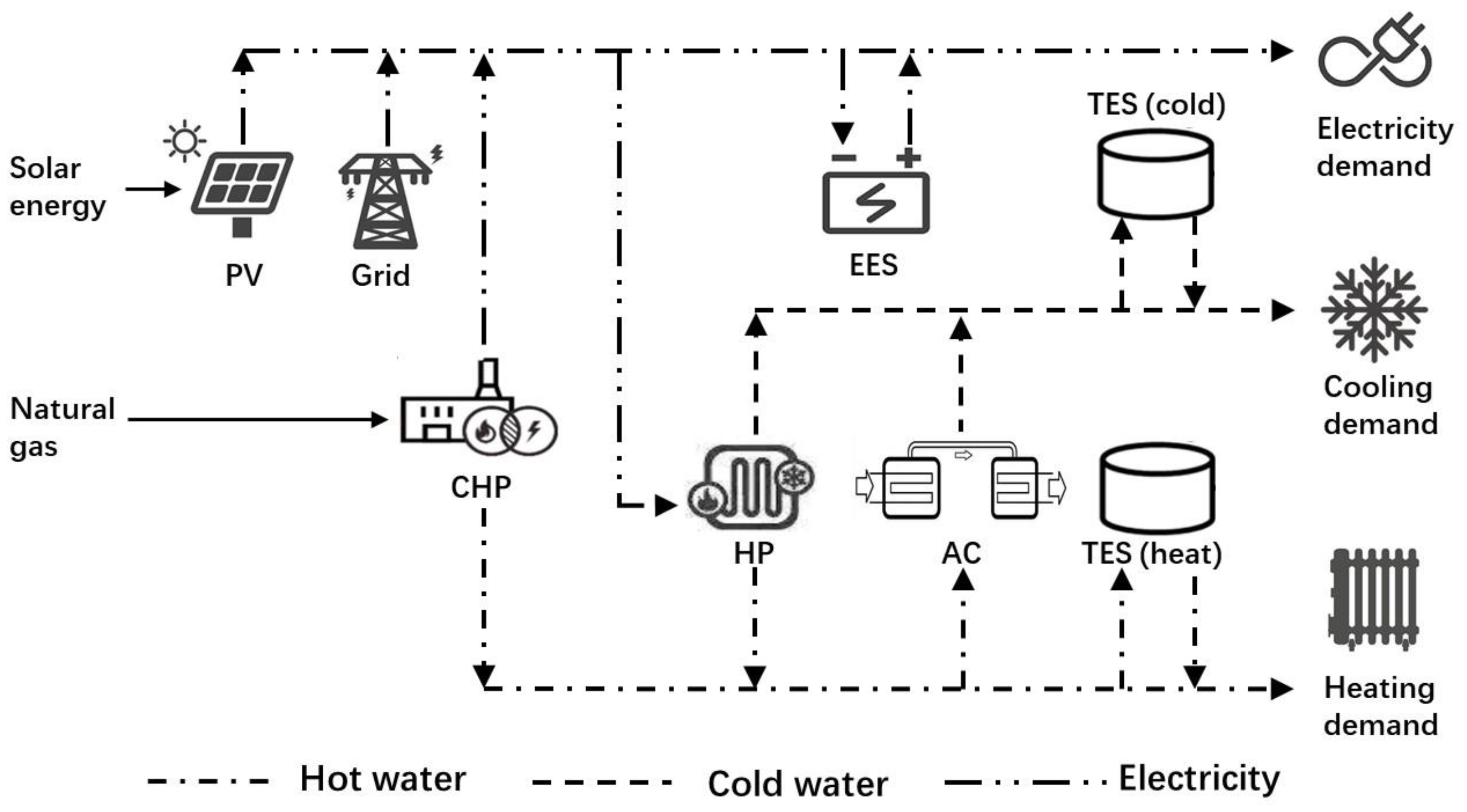
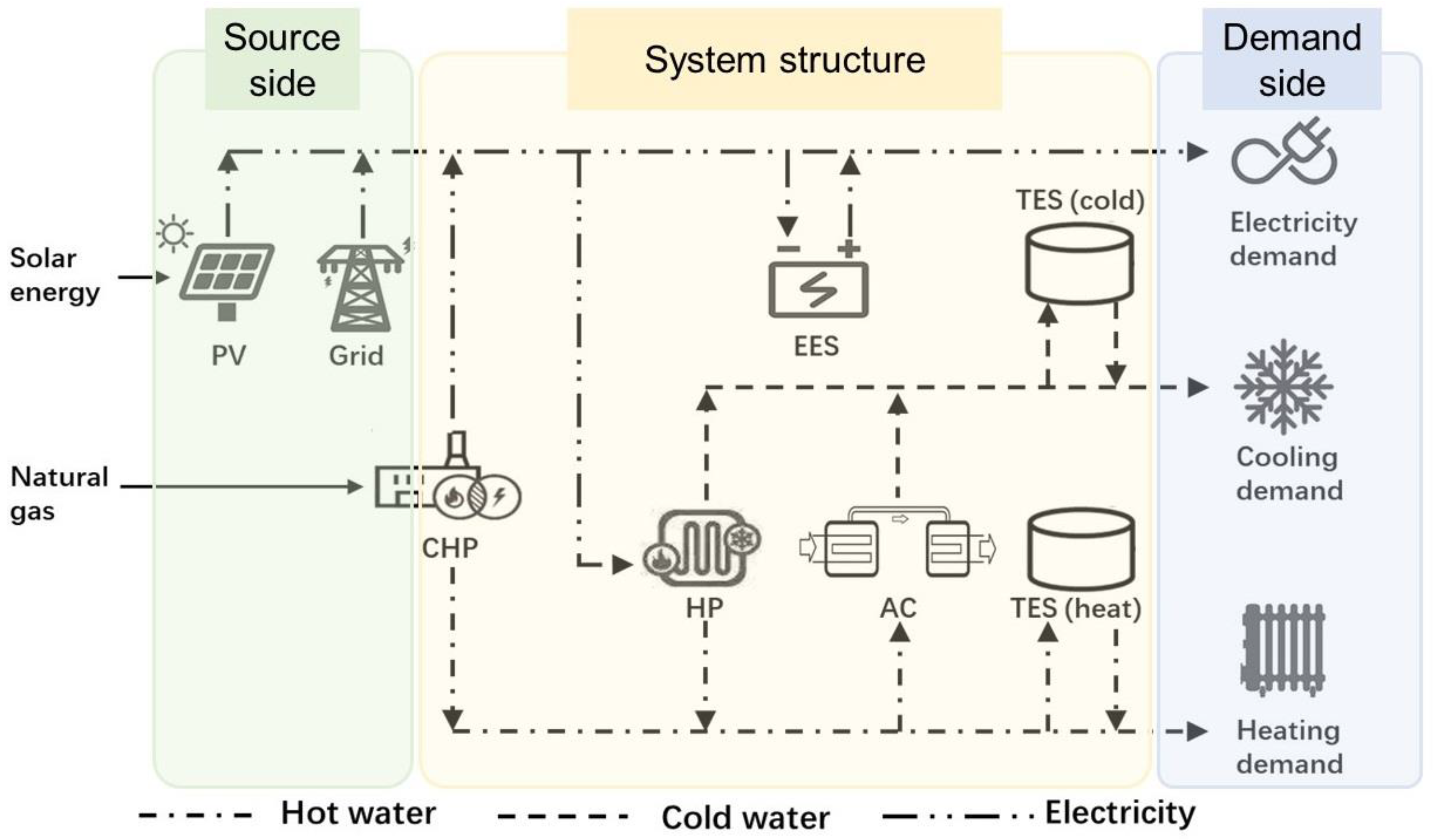
As shown in Figure 1, the IES consists of a photovoltaic (PV) unit, a CHP unit, a heat pump (HP) unit, an absorption chiller (AC) unit, a thermal energy storage (TES) system, an electric energy storage (EES) system, and energy demand for heat, cooling, and electricity.

2.2. System Flexibility Definition and Characteristics

With the increasing penetration of renewable energy, the uncertainty and volatility faced by IES are gradually increasing, which bring challenges to the flexibility of system operation scheduling. Currently, existing studies on flexibility mainly focus on the grid, especially on the “Generation–Distribution–Storage” chain. When addressing flexibility in energy systems, research remains in its infancy, and no consistent definition has been established.

At present, the definition of flexibility with high acceptance is based on grid flexibility, as proposed by the International Energy Agency (IEA) [37] and the North American Electric Reliability Council (NERC) [38]. The IEA defines flexibility as the ability to respond quickly to predictable and unpredictable fluctuations under boundary constraints—i.e., reducing supply within hours when demand decreases and increasing supply when demand rises. NERC characterizes flexibility as the grid’s capacity to use internal resources to meet demand fluctuations. In energy systems, definitions of system flexibility are context-specific, varying by application and perspective.

Generally, IES flexibility refers to the system’s adaptability to diverse scenarios. Building on previous definitions and characteristics, IES flexibility can be defined as a quantification of the system’s responsiveness and the risks of insufficient response over a specific time scale.

Therefore, the characteristics of IES flexibility can be summarized as follows:

• Time scale

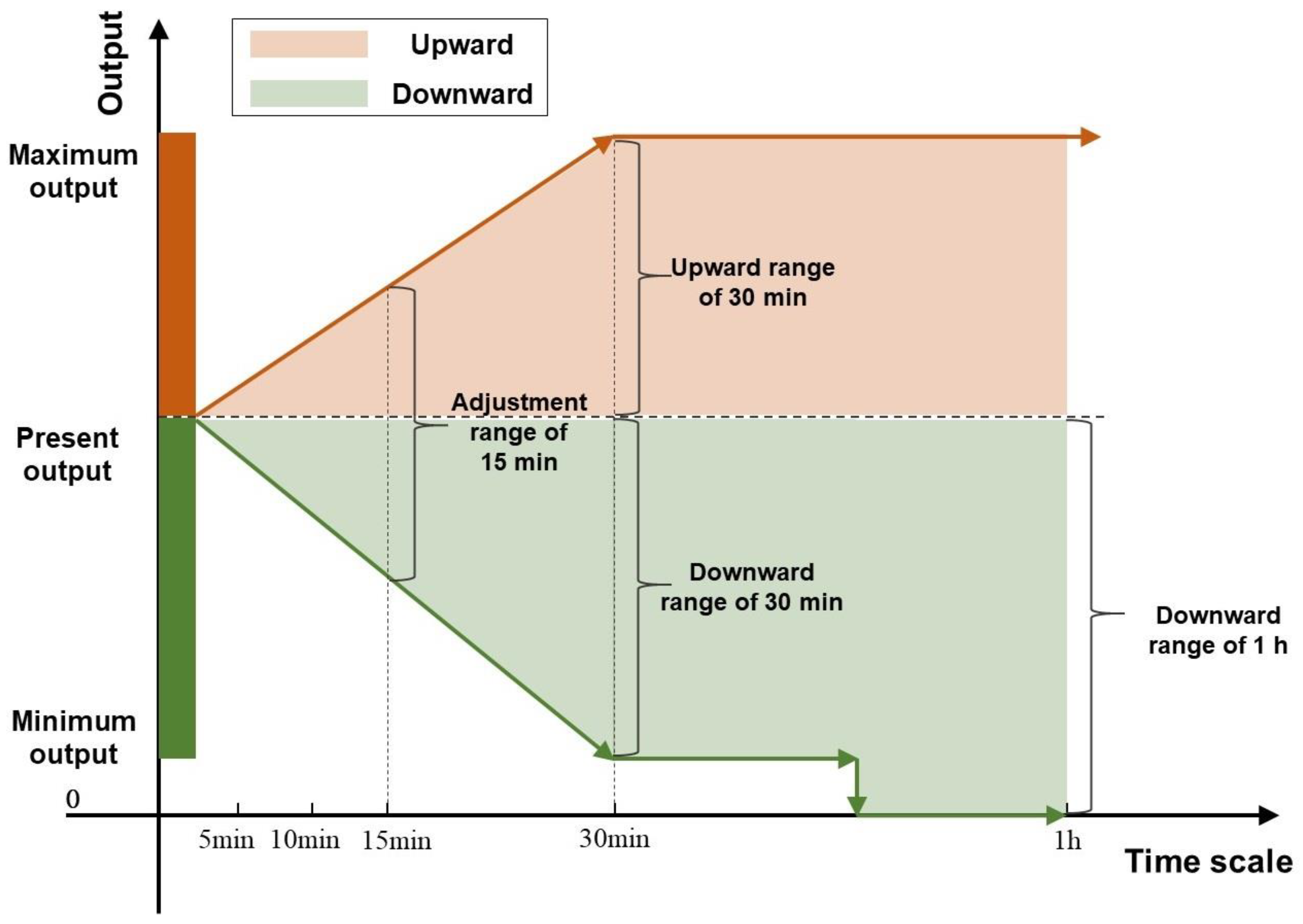
Flexible resources provided by equipment (e.g., energy storage) vary across time scales, with a strong correlation between resources and temporal dynamics. Thus, flexibility evaluation must occur within a defined time scale, making it a fundamental characteristic of flexibility.

IES flexibility time scales are categorized as fast (<15 min), medium (15 min–1 h), and slow (>1 h), as illustrated in Figure 2, which highlights differences across temporal dimensions.

2.

Directionality

Beyond time scale, directionality is another core characteristic of flexibility. During fluctuation response, equipment faces upward or downward power adjustment requirements, defining upward and downward flexibility. Upward flexibility denotes the capacity to increase equipment output, while downward flexibility reflects the ability to reduce output, as shown in Figure 2.

3.

Dependence on working state of the equipment

System flexibility is closely tied to equipment operating state, minimum and maximum output, and ramping rates—defining its key characteristics.

4.

Bidirectional convertibility

System flexibility depends on equipment states and can convert between upward and downward directions. Flexibility demand and supply are also convertible: e.g., renewable energy integration generates flexibility demand through fluctuations but can simultaneously provide flexibility supply. Similarly, while demand fluctuations create flexibility demand, reasonable demand response can supply flexibility to the system.

5.

Probabilistic Factors

As renewable energy penetration increases, there is a growing need to evaluate flexibility considering uncertainties. This requires flexibility metrics to incorporate uncertainty probability characteristics and enable system flexibility evaluation and optimization under uncertainty.

Figure 2. System flexibility characteristics.

Figure 2. System flexibility characteristics.

2.3. Flexibility Evaluation Index

With the advancement of IES, research on system flexibility should no longer solely focus on flexibility studies of specific equipment (e.g., energy storage) but instead adopt a multi-dimensional IES perspective—encompassing renewable energy, traditional energy, energy storage, and the energy demand side—to collectively address transition pressures and high flexibility development needs in the current energy landscape. Specifically, IES flexibility evaluation indexes should be derived from the system’s “Source–Structure–Demand” dimensions to establish a comprehensive evaluation framework, as illustrated in Figure 3.

This paper selects the Grid Dependency Level (GDL) for the source side, Insufficient Flexible Resource Probability (IFRP) for the structure side, and Loss of Load Probability (LOLP) for the demand side. Details of these indexes are as follows.

2.3.1. Grid Dependency Level (GDL)

In the grid interaction process, although power purchase and sale are subject to certain constraints, with the advancement of IES, extensive power transactions can pose challenges to grid stability. This concern is particularly pronounced during the current energy transition phase, as IES should avoid excessive reliance on grid interactions for flexibility and stability. The Grid Dependency Level (GDL) is introduced to quantify the degree of dependence on and interaction with the grid. A higher GDL value indicates that the system is highly reliant on the grid; its flexibility predominantly stems from grid support, while the internal flexibility of the system itself is limited, and its self-sufficiency is relatively weak. The mathematical definition of this index is presented in Equation (1):

$$GDL={\displaystyle {\sum }_{t=1}^T\frac{P_t^{grid,b}+P_t^{grid,s}}{P_t^{bl}},}\hspace{1em}\forall t\in \mathsf{{\rm T}}$$

(1)

where $t$ is the time step in the schedule period $\mathsf{{\rm T}}$, $\mathsf{{\rm T}}=\left[1,2,\cdots ,T\right]$; $P_t^{grid,b}$ and $P_t^{grid,s}$ are the amounts of electricity purchased from and sold to the grid; $P_t^{bl}$ is the system electricity demand.

2.3.2. Insufficient Flexible Resource Probability (IFRP)

When an IES encounters fluctuations stemming from uncertainties, it must respond promptly to maintain its stability and flexibility. However, the ramping rates of the equipment within the IES are relatively fixed. Consequently, during IES optimization, these equipment ramping rates should be meticulously considered to assess the system’s adaptability to uncertain fluctuations. To this end, Insufficient Flexible Resource Probability (IFRP) is chosen as the flexibility index for the system structure. This index comprehensively integrates the aspects of flexibility, stability, and security.

IFRP evaluates the adequacy of the system’s flexibility supply to meet its demands by considering the relationship between the Adjustment Margin of Flexible Resources (AMFR) and the Net Load Variation (NLV). A higher IFRP value signifies that it is more challenging for the system to supply sufficient flexibility, indicating a greater risk of flexibility shortages and lower system overall flexibility.

The definition and characteristics of IFRP suggest that its evaluation involves a two—step process. First, the NLV needs to be calculated. Subsequently, the AMFR within the system is determined.

6.

Net Load Volatility (NLV)

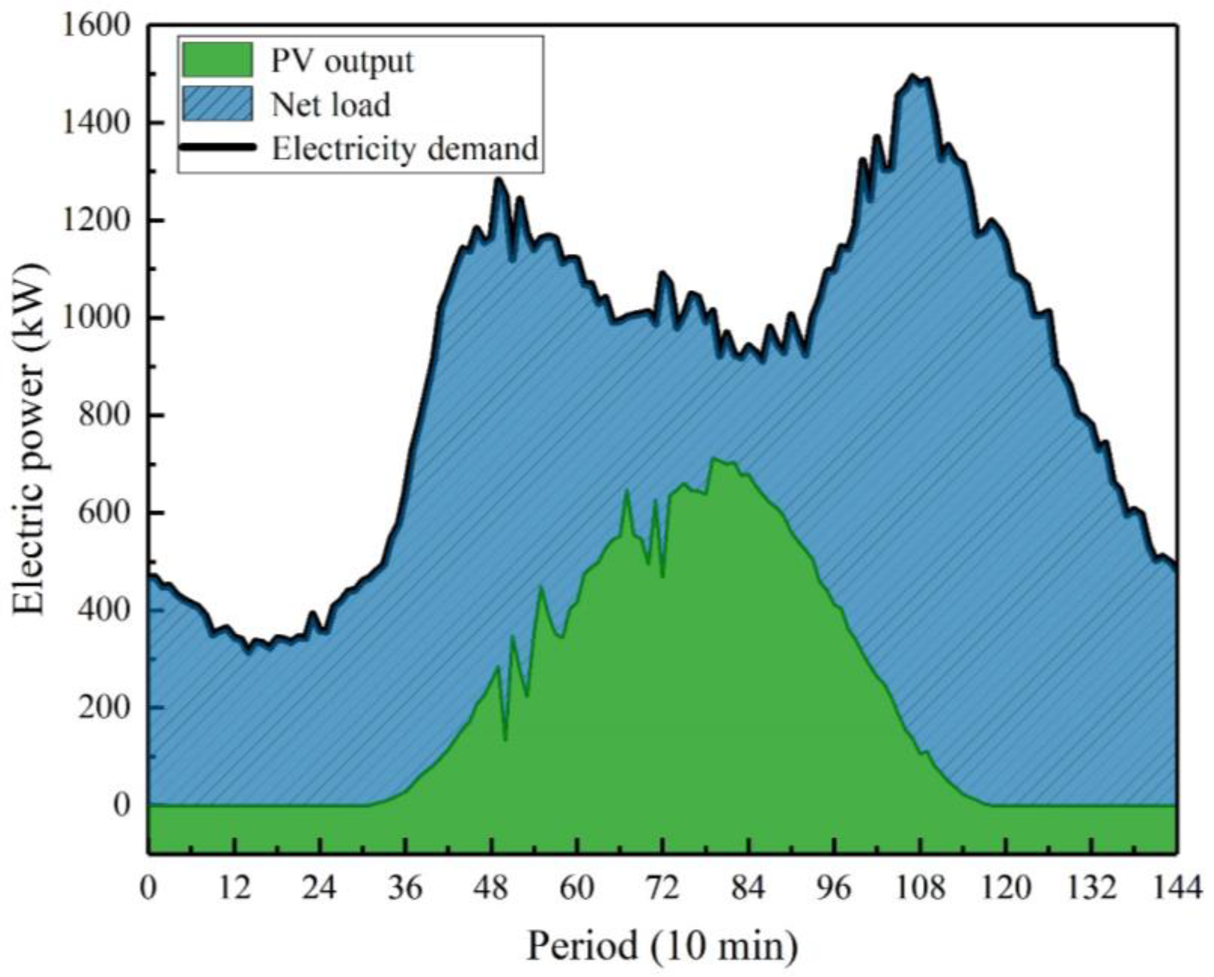
Net load $P_t^{NL}$ is the difference between the system electricity demand $P_t^{bl}$ and the output of renewable energy $P_t^{pv}$ on a certain time scale, as shown in Equation (2). Specifically, as Figure 4 shows, taking the 10 min time scale as an example, the blue area between the electricity demand and the PV output is the net load.

$$P_t^{NL}=P_t^{bl}-P_t^{pv},\hspace{1em}\forall t\in \mathsf{{\rm T}}$$

(2)

For the NLV, this refers to the net load subtraction at adjacent moments, as shown in the Equation (3).

$$NL{V}_t=P_{t+1}^{NL}-P_t^{NL},\hspace{1em}\forall t\in \mathsf{{\rm T}}$$

(3)

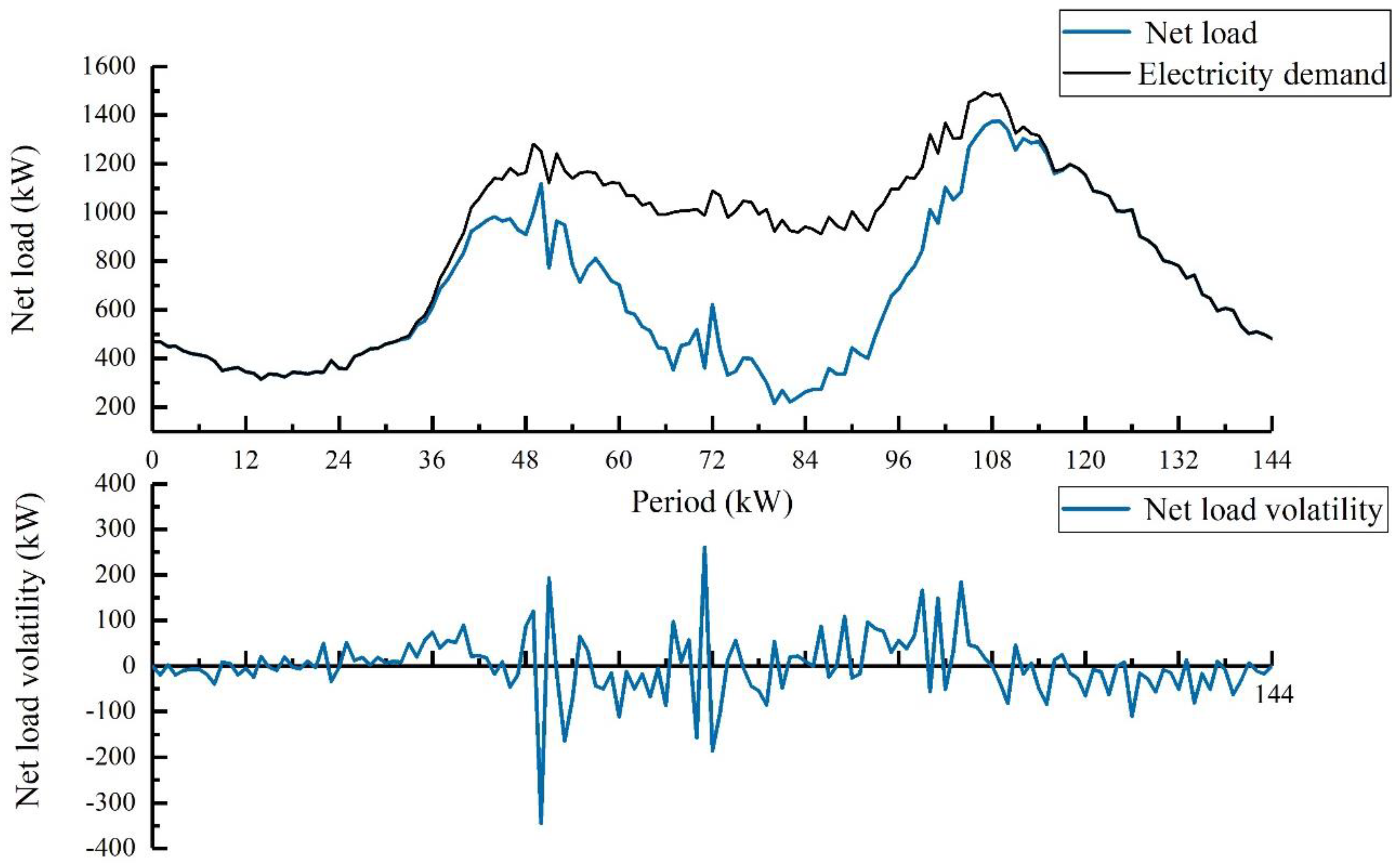
Within the IES, this metric effectively captures the system’s flexibility requirements. As illustrated in Figure 5, following the large-scale integration of renewable energy sources into the system, the amplitude of fluctuations in the net load becomes notably more pronounced compared to that of electricity demand. The net load curve exhibits two prominent characteristics: (1) a substantial dip around noon; (2) steeper ascending and descending slopes. These features suggest that when a high proportion of renewable energy is incorporated, the system must be equipped with adequate ramping capacity. Consequently, the system’s demand for flexibility has increased significantly.

Figure 5 also shows the NLV series. The positive and negative values of the NLV represent the direction of the flexibility demand. When the NLV is positive, it represents the upward flexibility demand of the system; when it is negative, it represents the downward flexibility demand of the system, which is expressed as follows:

$$\begin{array}{l}NL{V}^{+}=\left\{\left.NL{V}^{+}\right|NL{V}_t>0,\hspace{1em}\forall t\in \mathsf{{\rm T}}\right\}\\ NL{V}^{-}=\left\{\left.NL{V}^{-}\right|NL{V}_t<0,\hspace{1em}\forall t\in \mathsf{{\rm T}}\right\}\end{array}$$

(4)

For the upward and downward flexibility demand caused by NLV, the system needs to adjust internal flexible resources for flexibility supply. Combined with the flexibility characteristics shown in Figure 4, the AMFR refers to the upward flexibility margin and downward flexibility margin that can be provided to the system at a certain time within a certain time scale, as follows:

$$\begin{array}{l}AMF{R}_t^{+}=\min \left[(SO{C}_t-SO{C}_{\min })\cdot Ca{p}_{bat}, \mathsf{\Delta }t\cdot {\gamma }_{\max }^{bat,dis}\cdot Ca{p}_{bat}\right]\\ \hspace{1em}\hspace{1em}\hspace{1em}\hspace{1em}+{\displaystyle {\sum }_{i=1}^I\min (P_{\max }^i-P_t^i,\mathsf{\Delta }t\cdot ram{p}_{up}^i)},\hspace{1em}\forall t\in \mathsf{{\rm T}}\end{array}$$

(5)

$$\begin{array}{l}AMF{R}_t^{-}=\min \left[(SO{C}_{\max }-SO{C}_t)\cdot Ca{p}_{bat}, \mathsf{\Delta }t\cdot {\gamma }_{\max }^{bat,ch}\cdot Ca{p}_{bat}\right]\\ \hspace{1em}\hspace{1em}\hspace{1em}\hspace{1em}+{\displaystyle {\sum }_{i=1}^I\min (P_t^i-P_{\min }^i,\mathsf{\Delta }t\cdot ram{p}_{down}^i)},\hspace{1em}\forall t\in \mathsf{{\rm T}}\end{array}$$

(6)

where $SO{C}_t$ is the state of charge (SOC) of the EES at time $t$; $SO{C}_{\min }$ and $SO{C}_{\max }$ are the minimum and maximum SOC, respectively; $Ca{p}_{bat}$ is the EES’s capacity; $\mathsf{\Delta }t$ is the operation optimization time step; ${\gamma }_{\max }^{bat,ch}$ and ${\gamma }_{\max }^{bat,dis}$ are maximum charging and discharging rates of the EES; $P_t^i$ is the output power of the equipment $i$ which can provide flexible resources; $P_{\min }^i$ and $P_{\max }^i$ are the minimum and maximum output of equipment $i$; $ram{p}_{up}^i$ and $ram{p}_{down}^i$ are the upward and downward ramping rate of equipment $i$.

As mentioned before, NLV reflects the system’s flexible resource demand, and AMFR represents the flexible resource supply of the system. By comparing the magnitude of the upward (or downward) flexible resource demand and the upward (or downward) flexible resource supply, the insufficiency of the upward (or downward) flexible resource of the system can be obtained. The ratio of the situation of insufficient flexible resource to the flexibility resource demand NLV is IFRP. The expressions in Equations (7) and (8) are designed to make the value of IFRP positive for the convenience of subsequent calculations.

$$IFR{P}^{+}={\displaystyle {\sum }_{t=1}^T\frac{\max (NL{V}_t^{+}-AMF{R}_t^{+},0)}{NL{V}_t^{+}}}$$

(7)

$$IFR{P}^{-}={\displaystyle {\sum }_{t=1}^T\frac{\max (\left|NL{V}_t^{-}\right|-AMF{R}_t^{-},0)}{\left|NL{V}_t^{-}\right|}}$$

(8)

$$IFRP=\max (IFR{P}^{+},IFR{P}^{-})$$

(9)

2.3.3. Loss of Load Probability (LOLP)

The balance of energy supply and demand is the basic requirement of the IES operation process. Under the fluctuation of uncertainty, whether the system can meet the energy demand of the system is very crucial. The loss of load probability (LOLP) is used to evaluate the flexibility of the system demand side, while also reflecting the reliability of the system. A larger LOLP indicates that there are imbalances between supply and demand, and it is difficult to cope with the fluctuations of the system; moreover, it indicates that the flexibility reliability is weak. The expression of LOLP is as follows.

$$LOLP={\displaystyle {\sum }_{t=1}^T\frac{P_t^{st}}{P_t^{bl}}},\hspace{1em}\forall t\in \mathsf{{\rm T}}$$

(10)

where $P_t^{st}$ is the power shortage at time $t$ of the system as Equation (11) shows and, when it is positive, it represents the system’s power shortage:

$$P_t^{st}=(P_t^{bat,ch}+P_t^{hp}+P_t^{bl})-(P_t^{pv}+P_t^{gt}+P_t^{bat,dis}+P_t^{grid,b}-P_t^{grid,s}),\hspace{1em}\forall t\in \mathsf{{\rm T}}$$

(11)

where the first part is system power consumption and the second part is system power supply. Specifically, $P_t^{bat,ch}$ and $P_t^{bat,dis}$ represent the amount of charged and discharged electricity of EES; $P_t^{hp}$ and $P_t^{gt}$ are the output of HP and gas turbine of the CHP.

By homogenizing and weighting the above three side flexibility indexes, the system overall flexibility index $Flex$ can be obtained and used for system flexibility evaluation and system flexible optimization, etc. In order to improve the universality and applicability of the flexibility index framework, this paper adds weight factors to the flexibility indexes, as shown in Equation (12). The weight factors corresponding to the index represent the degree of emphasis placed on this dimension. The weight factors are numbered between 0 to 1, and the sum of all weight factors should be 1. If the value is larger, it indicates that the importance attached to this dimension is higher, i.e., the flexibility of the system is mainly concentrated at this dimension level. Therefore, the system designer can set the values of each weight factor by themselves according to the actual situation of the system and the operation scheduling goals, as long as the sum of the three weight factors is 1. In the case study of this paper, three weight factor are used with the same setting (a = b=c = 1/3), i.e., the importance of the three dimensions is the same.

$$\begin{array}{l}Flex=a\cdot GDL+b\cdot IFRP+c\cdot LOLP\\ \hfill (a+b+c=1)\hfill \end{array}$$

(12)

3. System Multi-Objective Optimization Model Considering Flexibility and Uncertainty

With the increasing penetration of renewable energy sources, IES exhibits significant uncertainties. These uncertainties pose risks to system operation and threaten its security. In response to the fluctuating uncertainties within the system, flexibility serves as a crucial guarantee for maintaining system security and reliability. Nevertheless, when flexibility reaches a certain threshold, the configuration and scheduling of flexible resources within the system encounter challenges, leading to a potential decline in security. Regarding system economy, enhancing flexibility generally has a positive impact on overall optimal scheduling and cost reduction. However, an excessive pursuit of high flexibility can drive the system into an extreme operational state, ultimately compromising its economic efficiency.

Therefore, optimizing IES requires a comprehensive consideration of diverse requirements. Multi-objective optimization, which takes into account economy, flexibility, security, and low carbon emissions, is highly imperative. In this paper, a multi-objective optimization model encompassing the aforementioned four aspects is established, with due consideration given to the high proportion of renewable energy integration and multiple uncertainties. During the operation of IES, different energy flows exhibit varying adjustment response times and inertia characteristics. For instance, electrical energy flow can respond instantaneously, while thermal energy flow is subject to thermal inertia. To address this disparity, thermal and electrical energy are optimized on distinct time scales, enabling the development of a multi-time scale, high-dimensional, non-convex, nonlinear model. This model facilitates the optimal configuration and flexible optimal scheduling of IES under complex conditions.

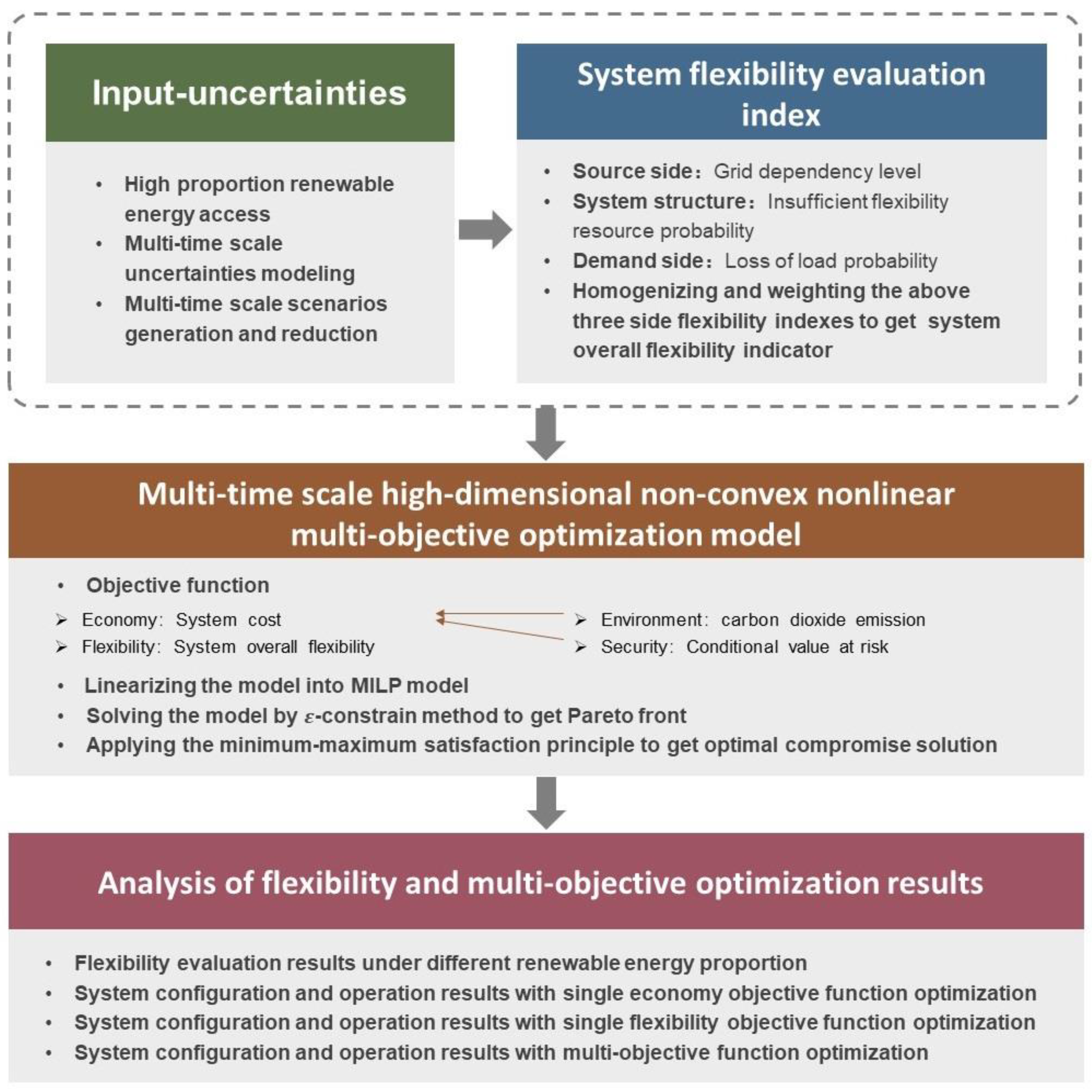
Prior to constructing the multi-objective optimization model, it is essential to model the multiple uncertainties. In this study, uncertainties related to renewable energy output and energy demand are considered. To handle these uncertainties, relevant uncertain parameters are modeled using stochastic programming methods. Subsequently, scenario generation and reduction processes are implemented, and the results are integrated into the system flexibility evaluation index. Finally, the multi-objective optimization model is optimized and solved, aiming to achieve the optimal configuration and flexible scheduling of IES with high renewable energy penetration. The specific framework is illustrated in Figure 6.

3.1. Objective Function of Optimization

The objective function of this optimization model contains four aspects: the economic aspect is system cost $SC$, the flexibility aspect is system overall flexibility $Flex$, the security aspect is conditional value at risk $CVaR$ and the environment aspect is carbon dioxide emission $CDE$. Considering the complexity of optimizing the four objective functions, the environmental objective $CDE$ is first transferred in the form of carbon taxes into the economic objective, and then the security objective $CVaR$ is transferred into an economic objective coupling with the weighting factor. Afterwards, two objective functions are determined in this multi-objective optimization model to pursue minimum system total cost $TC$ and maximum system flexibility (i.e., minimize the flexibility index value), as Equation (13) shows:

$$\begin{array}{l}{F}_1=\min TC\\ F_2=\min Flex\end{array}$$

(13)

$TC$ is the system total cost and is expressed as follows:

$$TC=E(SC+C^C)+\beta \cdot CVa{R}_{\alpha }(SC+C^C)$$

(14)

where $\beta$ is non-negative weight coefficient, representing the level of risk preference and reflecting the level of risk aversion of the system designer. When the value is 0–0.05, it represents the risk-seeking type, and when the value is greater than 0.1, it represents the risk-averse type. $\alpha$ is the confidence level. Detailed information about $CVaR$ can be found in article [39].

System cost $SC$ contains system equipment investment cost $C^I$, system maintenance cost $C^{OM}$ and system energy consumption cost $C^{OF}$. $C^C$ is the carbon tax. The following equations are detailed expressions:

$$SC=C^I+C^{OM}+C^{OF}$$

(15)

$$C^I={\displaystyle {\sum }_i\left[Ca{p}_i\cdot k_i\cdot \frac{I_p{(1+I_p)}^{d_i}}{{(1+I_p)}^{d_i}-1}\right]}$$

(16)

where $i$ refers to a particular type of equipment; $k$ represents the unit cost per capacity; $Cap$ denotes equipment capacity; $I_p$ is the interest rate; and $d$ is the service life:

$$C^{OM}={\displaystyle {\sum }_{t=1}^T\left[\begin{array}{l}{c}_m^{gt}\cdot P_t^{gt}+c_m^{hr}\cdot Q_t^{hr}+c_m^{ac}\cdot Q_t^{ac}+c_m^{pv}\cdot P_t^{pv}\\ +c_m^{hp}\cdot (Q_t^{hp,c}+Q_t^{hp,h})+c_{de}^{bat}\cdot (P_t^{bat,ch}+P_t^{bat,dis})\end{array}\right]}+c_m^{tes}\cdot Ca{p}_{tes},\hspace{1em}\forall t\in \mathsf{{\rm T}}$$

(17)

where $c_m^{gt}$, $c_m^{hr}$, $c_m^{ac}$, $c_m^{hp}$, $c_m^{pv}$, $c_{de}^{bat}$ and $c_m^{tes}$ are the per output maintenance cost for the gas turbine, heat recovery, AC, HP, PV, EES and TES, respectively; $Q_t^{hr}$, $Q_t^{ac}$, $Q_t^{hp,c}$ and $Q_t^{hp,h}$ are output of heat recovery, AC and HP, respectively.

$$C^{OF}={\displaystyle {\sum }_{t=1}^T\left(p_g\cdot F_t^{gas}+p_{buy}^{grid}\cdot P_t^{grid,b}-p_{sell}^{grid}\cdot P_t^{grid,s}\right)},\hspace{1em}\forall t\in \mathsf{{\rm T}}$$

(18)

where $p_g$ is the price for natural gas; $F_t^{gas}$ is the natural gas consumption; $p_{buy}^{grid}$ is the price of buying electricity from the grid, and $p_{sell}^{grid}$ is the price for selling electricity to the grid.

$$C^C=c_c\cdot {\displaystyle {\sum }_{t=1}^T(CD{E}^{grid}\cdot P_t^{grid,b}+CD{E}^{gas}\cdot F_t^{gas}),\hspace{1em}\forall t\in \mathsf{{\rm T}}}$$

(19)

where $c_c$ is carbon tax; and $CD{E}^{grid}$ and $CD{E}^{gas}$ are the carbon dioxide emission factors of the grid and natural gas, respectively.

3.2. Constraints on Optimization

The optimization model’s constraints contain equipment operating constraints and energy balance.

The constraints on the CHP include the following:

$$P_t^{gt}=F_t^{gas}\cdot H_{ng}\cdot {\eta }_{egt},\hspace{1em}\forall t\in \mathsf{{\rm T}}$$

(20)

$$Q_t^{gt}=F_t^{gas}\cdot H_{ng}\cdot (1-{\eta }_{egt}-{\eta }_s),\hspace{1em}\forall t\in \mathsf{{\rm T}}$$

(21)

$$Q_t^{hr}=Q_t^{gt}\cdot {\eta }_{hr},\hspace{1em}\forall t\in \mathsf{{\rm T}}$$

(22)

where $H_{ng}$ is the calorific value of natural gas; ${\eta }_{egt}$ is the efficiency of CHP generating electricity and ${\eta }_s$ is the dissipative coefficient; ${\eta }_{hr}$ is the efficiency of heat recovery; and $Q_t^{gt}$ is the thermal output of gas turbine.

The CHP must adhere to the operational constraints regarding the minimum output $P_{\min }^{gt}$ and maximum output $P_{\max }^{gt}$, the ramp-up rate $\mathsf{\Delta }{P}_{up}^{gt}$ and ramp-down rate $\mathsf{\Delta }{P}_{down}^{gt}$, and the minimum interval $\mathsf{\Delta }{t}^{gt}$ between start and stop, as indicated by Equations (23)–(25).

$$P_{\min }^{gt}\le P_t^{gt}\le P_{\max }^{gt},\hspace{1em}\forall t\in \mathsf{{\rm T}}$$

(23)

$$-\mathsf{\Delta }{P}_{down}^{gt}\le P_{t+1}^{gt}-P_t^{gt}\le \mathsf{\Delta }{P}_{up}^{gt},\hspace{1em}\forall t\in \mathsf{{\rm T}}$$

(24)

$$\mathsf{\Delta }{t}^{gt}\ge \mathsf{\Delta }{t}_{\min }^{gt}$$

(25)

The constraints on the absorption chiller and heat pump include the following:

$$Q_t^{ac}=Q_t^{hr}\cdot CO{P}_{ac},\hspace{1em}\forall t\in \mathsf{{\rm T}}$$

(26)

$$Q_t^{hp,h}=P_t^{hp,h}\cdot CO{P}_h^{hp},\hspace{1em}\forall t\in \mathsf{{\rm T}}$$

(27)

$$Q_t^{hp,c}=P_t^{hp,c}\cdot CO{P}_c^{hp},\hspace{1em}\forall t\in \mathsf{{\rm T}}$$

(28)

where $P_t^{hp,c}$ and $P_t^{hp,h}$ are the electricity consumption of the heat pump in cooling and heating mode; and $CO{P}_{ac}$, $CO{P}_c^{hp}$ and $CO{P}_h^{hp}$ are the COPs of the AC and heat pump for cooling and heating, respectively. The AC and HP also need to adhere to the working minimum and maximum output constraints and HP cannot work in cooling mode and heating mode at the same time.

The constraints on the EES and TES include the following:

$$SO{C}_{t+1}\cdot Ca{p}_{bat}=SO{C}_t\cdot Ca{p}_{bat}+P_t^{bat,ch}\cdot {\eta }_{ch}^{bat}-P_t^{bat,dis}/{\eta }_{dis}^{bat},\hspace{1em}\forall t\in \mathsf{{\rm T}}$$

(29)

$$SO{T}_{t+1}\cdot Ca{p}_{tes}=(1-{\delta }_{tes})\cdot SO{T}_t\cdot Ca{p}_{tes}+Q_t^{tes,ch}\cdot {\eta }_{ch}^{tes}-Q_t^{tes,dis}/{\eta }_{dis}^{tes}, \forall t\in \mathsf{{\rm T}}$$

(30)

where SOC represents the state of charge (SOC) of the EES; ${\eta }_{ch}^{bat}$ and ${\eta }_{dis}^{bat}$ are the charging and discharging efficiency of EES, respectively; SOT is the state of TES; ${\delta }_{tes}$ is the self-discharging rate of the TES; ${\eta }_{ch}^{tes}$ and ${\eta }_{dis}^{tes}$ are its charging and discharging efficiency of TES, respectively. The EES’s and TES’s charging and discharging cannot exceed the limitation; detailed expression can be seen in [40].

The constraints regarding energy balance include the following:

Electricity energy balance:

$$P_t^{pv}+P_t^{gt}+P_t^{bat,dis}+P_t^{grid,b}-P_t^{grid,s}=P_t^{bat,ch}+P_t^{hp}+P_t^{bl},\hspace{1em}\forall t\in \mathsf{{\rm T}}$$

(31)

Heating energy balance:

$$Q_t^{hp,h}+Q_t^{hr}+Q_t^{tes,dis}\ge Q_t^{tes,ch}+Q_t^{bl,h},\hspace{1em}\forall t\in \mathsf{{\rm T}}$$

(32)

Cooling energy balance:

$$Q_t^{ac}+Q_t^{hp,c}+Q_t^{tes,dis}\ge Q_t^{tes,ch}+Q_t^{bl,c},\hspace{1em}\forall t\in \mathsf{{\rm T}}$$

(33)

where $Q_t^{bl,h}$ and $Q_t^{bl,c}$ are heating demand and cooling demand, respectively.

The multi-objective optimization model can be expressed as follows:

$$\left\{\begin{array}{l}{F}_1=\min TC\\ F_2=\min Flex\\ s.t. Eq.(20)-Eq.(33)\end{array}\right.$$

(34)

3.3. Method for Solving Optimization

Commonly used methods for solving multi-objective optimization models include the linear weighted method, $\epsilon$-constraint method, objective programming approach, etc. In this paper, the $\epsilon$-constraint method was chosen to solve the model. The $\epsilon$-constraint method converts the other objective functions, except one, into constraints, these constraints are limited by special parameter $\epsilon$, and then the solution is iterated under different $\epsilon$ levels to obtain the Pareto front of the original multi-objective function.

In this paper, we converted $F_2$ into constraints and Equation (34) was transferred into:

$$\left\{\begin{array}{l}\min F_1\\ s.t. F_2\le \epsilon \\ \hspace{1em}Eq.(20)-Eq.(33)\end{array}\right.$$

(35)

The $\epsilon$ in Equation (35) varies from the maximum value to the minimum value of $F_2$ successively, and the Pareto front is the set of solutions of all variations in the value of $\epsilon$. The value of $\epsilon$ is as follows:

$$\epsilon =F_{2,\max }-(F_{2,\max }-F_{2,\min })\cdot {\displaystyle \frac{ci-1}{cn-1}}$$

(36)

where $F_{2,\max }$ is the value of $F_2$ obtained when the system economic objective function $F_1$ is the single objective of optimization; $F_{2,\min }$ is the value of $F_2$ obtained when the system flexibility objective function $F_2$ is the single objective of optimization; $ci$ is the number of cycle iterations, and $ci=1,2,\cdots cn$, $cn$ is the maximum number of cycles.

After obtaining the Pareto solution frontier through the $\epsilon$-constraint method, this paper adopted a fuzzy decision-making method to select the optimal compromise solution from the Pareto front. This fuzzy decision-making method is based on judging the relative dominance relationship in the Pareto solution set.

Specifically, firstly, the fuzzy membership function degree $\kappa$ is obtained by handling the solution sets of different objective functions, and the expression is as follows:

$${\kappa }_m^{si}=\left\{\begin{array}{ll}1 ,& F_m^{si}<F_{m,\min }\\ {\displaystyle \frac{F_{m,\max }-F_m^{si}}{F_{m,\max }-F_{m,\min }}} ,& F_{m,\min }\le F_m^{si}\le F_{m,\max }\\ 0 ,& F_m^{si}>F_{m,\max }\end{array}\right.$$

(37)

where $si$ represents the $si$-th solution, $si=1,2,\cdots cn$; $m$ is the $m$-th objective function, $m=1,2$; ${\kappa }_m^{si}$ is the membership degree of the $m$-th objective function under the $si$-th solution; $F_m^{si}$ is the value of the $m$-th objective function in the $si$-th solution; and $F_{m,\max }$ and $F_{m,\min }$ are the maximum and minimum values of the $m$-th objective function, respectively.

Afterwards, the optimal compromise solution is obtained by applying the minimum–maximum satisfaction principle to the fuzzy membership function degree. At first, the membership degree under the two objective functions of the $si$-th solution is compared, the minimum value of which is selected as the membership degree ${\kappa }^{si}$ under the $si$-th solution, and then the membership degrees in all solutions are compared. Finally, the solution corresponding to the maximum value is selected as the optimal compromise solution, as shown in the following equation:

$$\begin{array}{l}{\kappa }^{si}=\min ({\kappa }_1^{si},{\kappa }_2^{si})\\ {\kappa }^{\max }=\max ({\kappa }^1,{\kappa }^2,\cdots {\kappa }^{cn})\end{array}$$

(38)

This paper aims to establish a multi-time scale high-dimensional non-convex nonlinear multi-objective optimization model that takes flexibility and uncertainty into account. The multi-time scale optimization is based on the different balance constraints of electrical energy and thermal energy in order to carry out a synchronous optimization structure.

In order to enhance the universality of the model, a widely used and recognized method, stochastic programming, was used to describe these uncertainties, and scenario theory was applied for solution. Specifically, the probability density function (PDF) description is established according to the historical distribution characteristics of uncertainty parameters. Then, according to the PDF, the scenarios are generated by Latin Hypercube Sampling method. After scenario generation, the simultaneous backward reduction method is used to reduce the scenario aggregation. Finally, the model can be solved. The detailed method description of modelling and integration can be seen in [2].

The whole optimization problem solving flowchart is as shown in Figure 7.

4. Case Study

In view of the more complex energy using pattern of residential buildings, more diverse changes, and relatively high demand for flexibility, this paper chose a high-rise apartment residential community buildings in Jinan, a city in northern China, as case study object. Taking the data of Jinan as an example for case analysis, the model proposed in this paper can be used normally if the data are changed for other cities. A typical summer day is selected as an example to carry out optimization analysis. The climate data were sourced from the open data platform METEONORM. The demand data are obtained through simulation using simulation software TRNSYS.

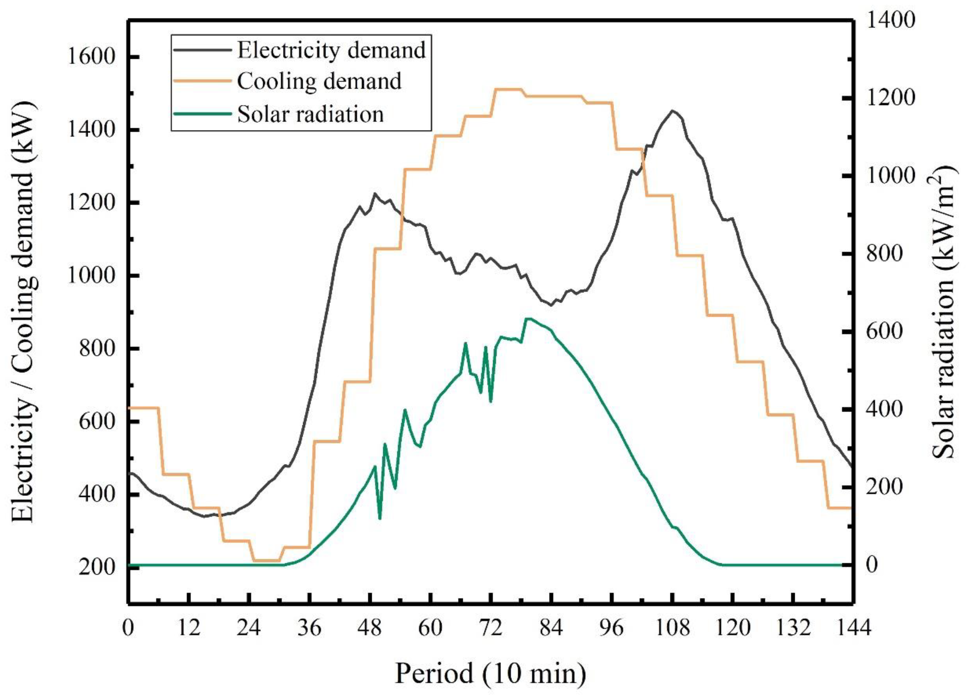
Considering the thermal inertia of thermal energy and the immediate demand for electric energy during the system operation, the optimization of thermal energy and electric energy is modeled on different time scales, respectively. In this paper, electric energy is on a 10-min scale and thermal energy a 1 h scale, 24 h is selected as the operation cycle due to the periodicity of energy consumption, and renewable energy penetration rate is 50%; detailed energy demand and solar radiation intensity are shown in Figure 8. Energy prices are shown in

Table 1. Energy price.

	Time	Price
Peak-valley electricity purchase price	7:00–8:00	0.6259 RMB/kWh
	8:00–11:00	0.9243 RMB/kWh
	11:00–16:00	0.6259 RMB/kWh
	16:00–21:00	0.9243 RMB/kWh
	21:00–23:00	0.6259 RMB/kWh
	23:00–7:00 (day + 1)	0.3275 RMB/kWh
Peak-valley electricity purchase price (July–September)	7:00–8:00	0.6259 RMB/kWh
	8:00–10:00	0.9243 RMB/kWh
	10:00–11:00	1.0437 RMB/kWh
	11:00–16:00	0.6259 RMB/kWh
	16:00–19:00	0.9243 RMB/kWh
	19:00–21:00	1.0437 RMB/kWh
	21:00–23:00	0.6259 RMB/kWh
	23:00–7:00 (day + 1)	0.3275 RMB/kWh
Natural gas price	/	2.3 RMB/m3

Source: obtained from [41,42].

, and technical details of the main system components can be seen in

Table 2. Technical details of main system components.

Parameter	Value	Parameter	Value
Electric energy storage		Coefficient of performance	0.7
Unit depreciation cost (RMB/kWh)	0.1	Heat pump
Maximum charging rate	0.20	Coefficient of performance (cooling)	5
Maximum discharge rate	0.40	Coefficient of performance (heating)	4.5
Charge efficiency	0.95	Minimum start-stop interval (h)	3
Discharge efficiency	0.95	Minimum working rate	0.1
SOCmin	0.20	Maximum output power (kW)	2000
SOCmax	0.95	Thermal energy storage
Gas turbine		Unit maintenance cost (RMB/m3)	40
Carbon dioxide emission factors (kg/m3)	1.96	Coefficient of heat transfer or cold	0.04
Unit maintenance cost (RMB/kWh)	0.05	Heat input efficiency	0.98
Calorific value of natural gas (kWh/m3)	9.78	Heat output efficiency	0.98
Efficiency of generating electricity	0.3	Cooling input efficiency	0.98
Dissipative coefficient	0.2	Cooling output efficiency	0.98
Minimum start-stop interval (h)	2	Grid
Maximum output power (kW)	2000	Carbon dioxide emission factors (kg/kWh)	0.872
Minimum output power (kW)	100	Carbon tax
Absorption chiller		Price (RMB/kg)	0.06
Unit maintenance cost (RMB/kW)	0.02

Source: obtained from [43,44,45].

.

5. Results and Discussion

Results are reported in this section to analyze the system flexibility evaluation and multi-objective optimization.

5.1. Results of Single Economy Objective Function Optimization

In this paper, a single economy objective function optimization was conducted to evaluate system overall flexibility and optimize system configuration and operation. These results serve as the benchmark model for subsequent analyses.

Table 3. System cost, capacity and system overall flexibility results of single economy objective optimization.

	System Total Cost	System Overall Flexibility		Carbon Tax	CVaR
Value	17,425 RMB	0.262		5686 RMB	16,234 RMB
Capacity
Gas turbine			690 kW
AC			830 kW
HP			1450 kW
EES			1300 kWh
TES			720 kWh

presents the total system cost, equipment capacity, and system overall flexibility obtained from the single economy objective optimization. The findings indicate that, under the objective of minimizing system cost, the gas turbine is selected as the primary energy supply equipment. This choice simultaneously achieves economic efficiency and a certain degree of flexible adjustment, with the remaining energy demand met by the power grid and PV. However, the randomness and volatility of PV power generation negatively impact the system’s flexibility. Moreover, the high reliance on the power grid increases the system’s dependence on external sources, thereby restricting its inherent flexibility development. The calculated system overall flexibility from the optimization results is 0.262, which is relatively large and indicative of a lower level of system flexibility.

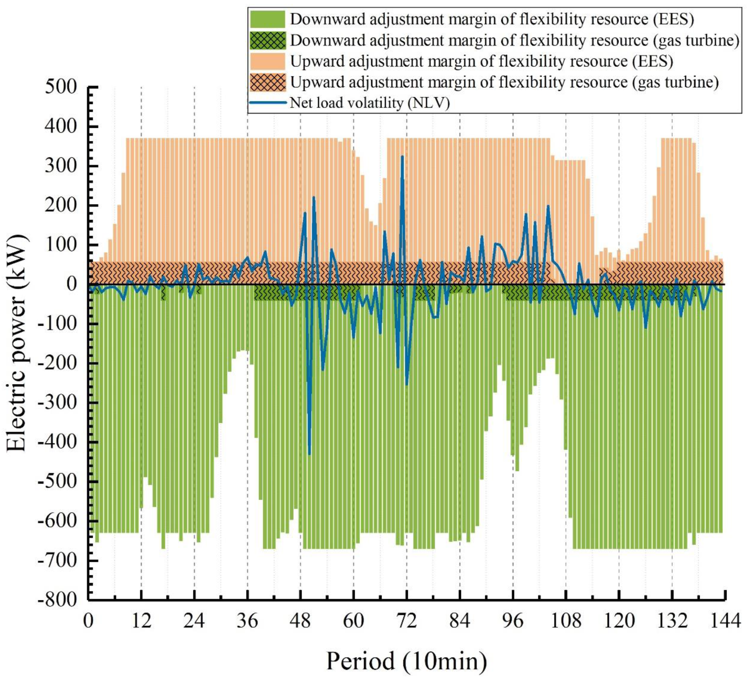
To further analyze the system’s flexibility, Figure 9 illustrates the comparison between the system’s NLV and AMFR to reflect the flexibility adequacy on the 10-min time scale. As depicted in Figure 9, the system’s flexibility margin significantly exceeds the flexibility demand, suggesting that the system possesses ample upward and downward flexibility within this time frame. Nevertheless, considering the aforementioned grid dependence, the overall flexibility of the system remains limited. Additionally, by comparing the margin contributions of the two types of flexible resources, it is evident that the energy storage system plays a more pivotal role in enhancing the system’s flexibility. Leveraging the flexible adjustment capabilities of electric energy storage is crucial for maintaining system stability. This also underscores the importance of comprehensively considering the allocation level of flexible resources during system configuration optimization.

5.2. Results of the Single Flexibility Objective Function Optimization

Upon analyzing the results of the single economy objective optimization, it is evident that there is room for improving the system’s flexibility. Consequently, a single flexibility objective optimization was carried out, and the optimized results are presented in Table 4. A comparison with the results in Section 5.1 reveals the following:

(1)

Driven by the objective of enhancing flexibility, the system’s flexibility has been significantly improved; however, this improvement has come at the expense of a certain degree of reduction in system economy. Specifically, the system cost has increased by 49.3%. This outcome aligns with the analysis in Section 3, indicating that an excessive pursuit of system flexibility significantly impacts its economic performance.

(2)

While improving the system’s flexibility, there has been a negligible reduction in carbon emissions. This can be attributed to the decreased interaction with the power grid and the reduced electricity procurement from external sources.

(3)

Regarding system security, similar to the trend observed in economic variation, the system’s CVaR has increased by 51.1%. This suggests that an excessive focus on flexibility and frequent operational adjustments have a detrimental impact on system security.

(4)

In terms of system equipment capacity, as flexibility improves, the capacity has been augmented to meet the requirements of flexible adjustments, enabling more versatile resource scheduling. The decrease in the capacity of the HP is due to the increased capacity of the air conditioner AC, a complementary cooling equipment, which subsequently reduces the demand for HP to a certain extent.

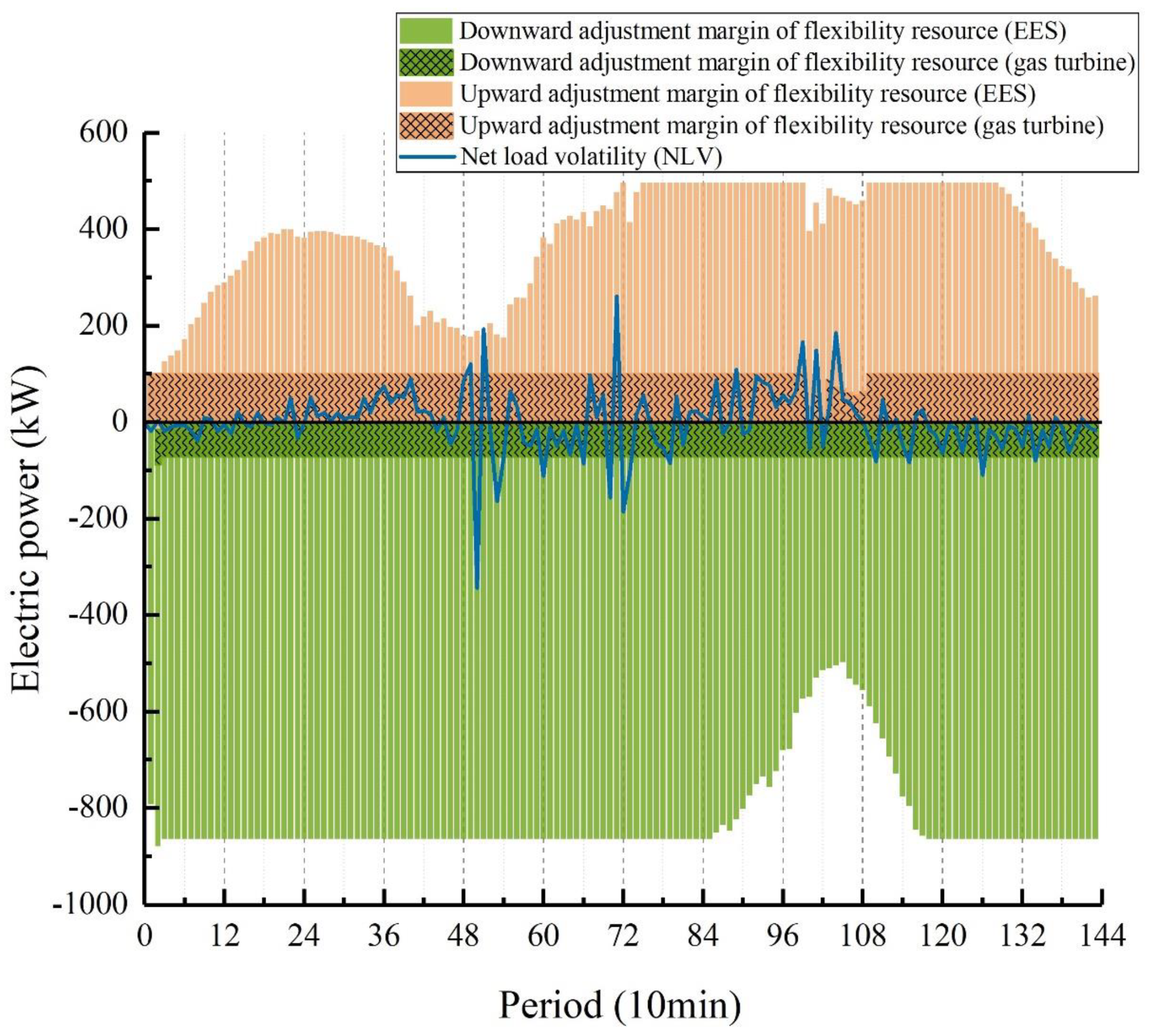
Furthermore, to demonstrate the system’s flexibility adequacy on the 10-min time scale, Figure 10 provides detailed results. Under the same system flexibility demand, the single flexibility objective optimization results show the following:

(1)

The AMFR of the gas turbine increases as its capacity grows, and the flexibility margin is more stable, both in the upward and downward directions, compared to the results under the economy objective optimization.

(2)

For the primary flexible resource provider, the EES system, it is evident from the figure that it offers a higher and more stable flexible resource margin for system flexibility. The peak of the downward flexibility margin has increased from 560 kW to 860 kW, representing a 53.6% increase, while the peak of the upward flexibility margin has risen from 320 kW to 500 kW, a 56.3% increase.

(3)

Compared with the economy optimization results, the margin values are not only larger but also more stable, ensuring a consistent supply of flexible resources to the system. This also highlights the potential for the system to accommodate a higher proportion of renewable energy, thereby meeting the flexibility demands arising from increased fluctuations.

The analysis of the single flexibility objective optimization results underscores that an excessive pursuit of flexibility compromises the system’s economic and security performance. This emphasizes the necessity of multi-objective flexibility optimization. In future optimization endeavors, attention should be paid to the coordinated optimization of multiple objectives to achieve balanced system development.

Table 4. System cost, capacity and system overall flexibility results of single flexibility objective optimization.

	Single Economy Objective Optimization	Single Flexibility Objective Optimization
System total cost (RMB)	26,023	17,425
Flexibility	0.0426	0.262
Carbon tax (RMB)	4563	5686
CVaR (RMB)	24,512	16,234
Gas turbine capacity (kW)	1200	690
AC capacity (kW)	1300	830
HP capacity (kW)	880	1450
EES capacity (kWh)	1980	1300
TES capacity (kWh)	2000	720

Table 4. System cost, capacity and system overall flexibility results of single flexibility objective optimization.

	Single Economy Objective Optimization	Single Flexibility Objective Optimization
System total cost (RMB)	26,023	17,425
Flexibility	0.0426	0.262
Carbon tax (RMB)	4563	5686
CVaR (RMB)	24,512	16,234
Gas turbine capacity (kW)	1200	690
AC capacity (kW)	1300	830
HP capacity (kW)	880	1450
EES capacity (kWh)	1980	1300
TES capacity (kWh)	2000	720

Figure 10. System net load volatility and single flexibility objective optimization’s flexible resources adjustment margin.

Figure 10. System net load volatility and single flexibility objective optimization’s flexible resources adjustment margin.

5.3. Flexibility Evaluation Results Under Different Renewable Energy Penetration Rates

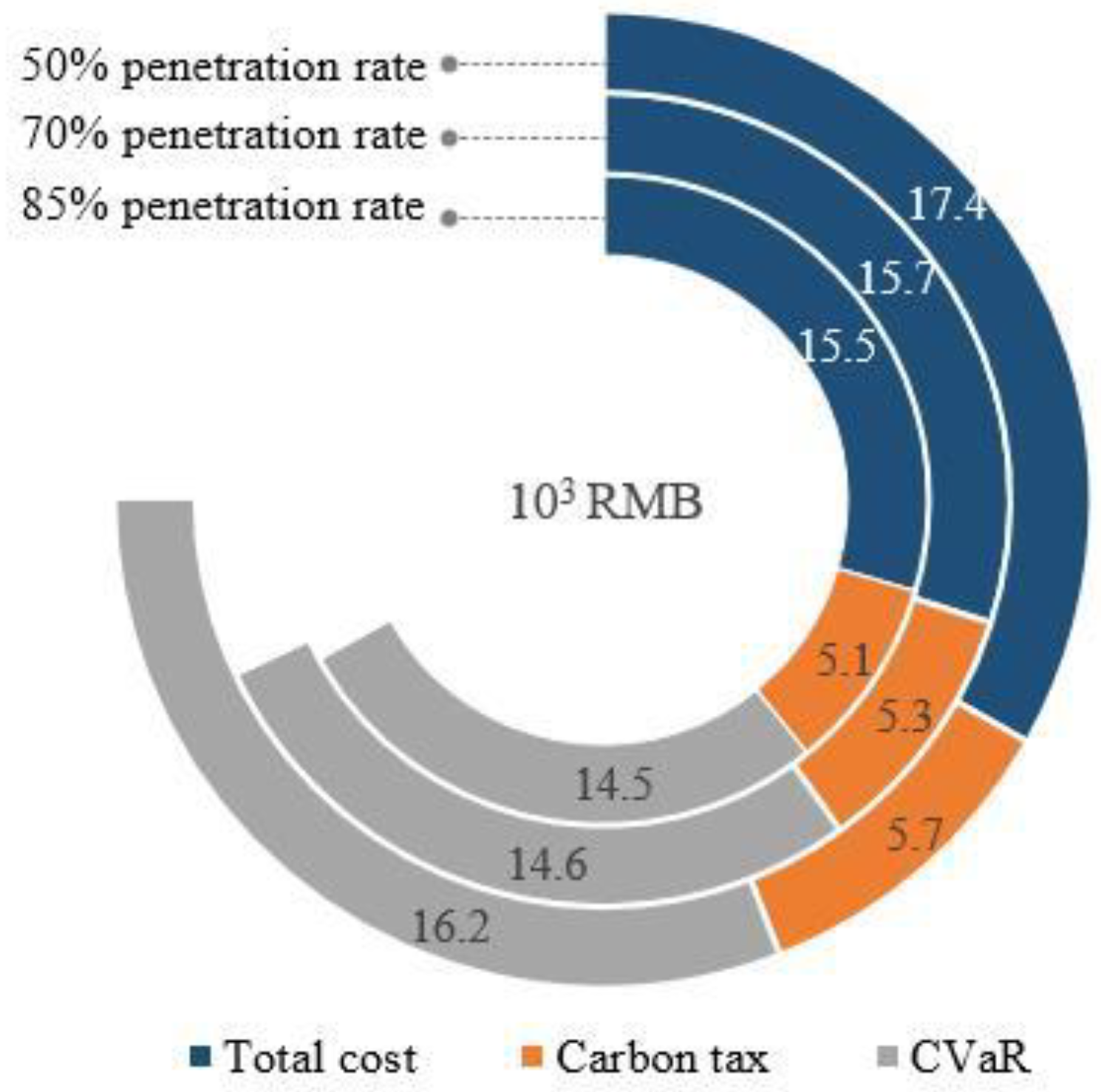
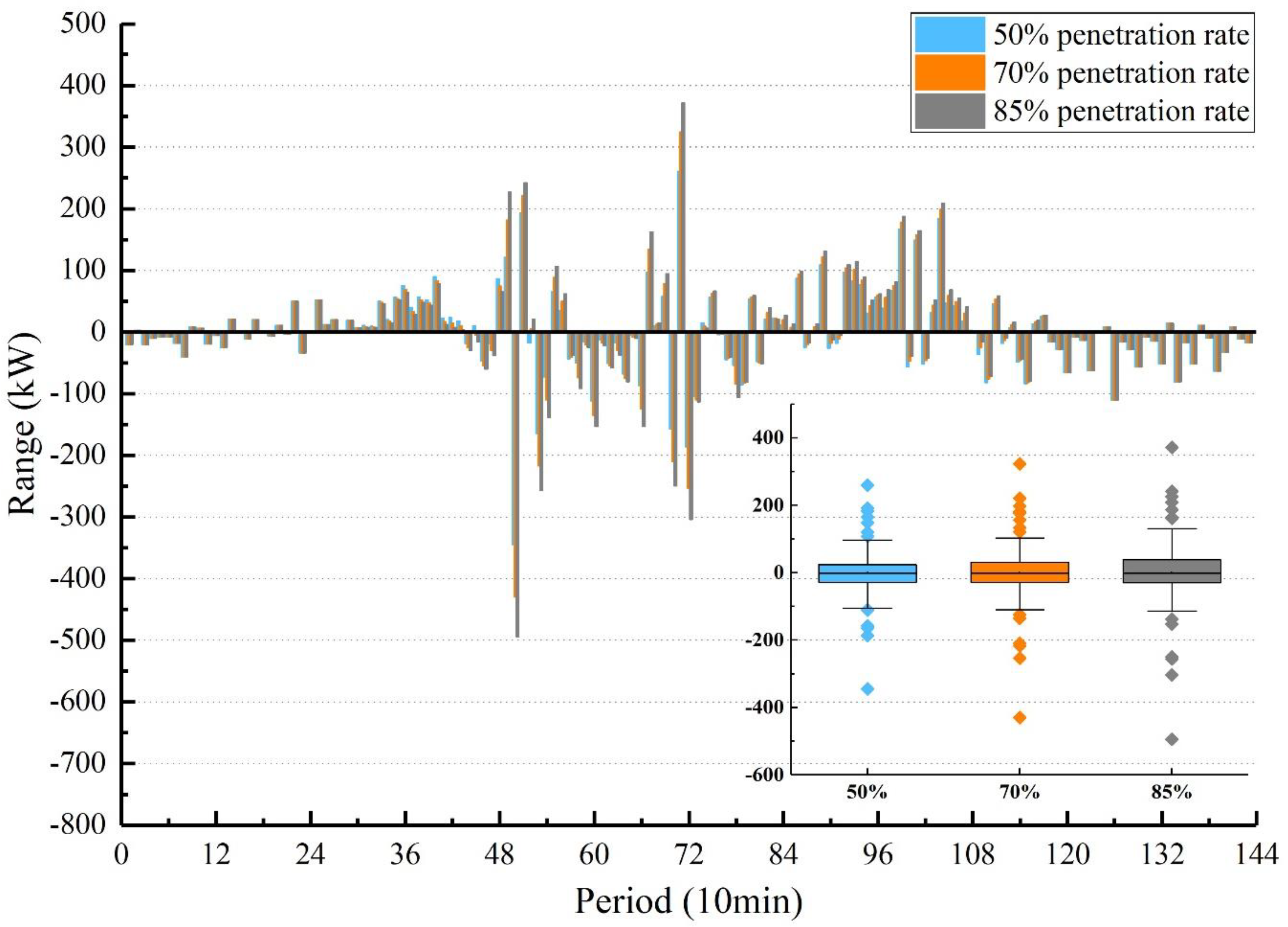
To investigate the influence of high-proportion renewable energy integration on system flexibility and optimization outcomes, this section constructs scenarios with 50%, 70%, and 85% renewable energy penetration rates, building upon the findings of previous sections. Figure 11 illustrates the system cost, carbon tax, and CVaR under varying penetration rates. Figure 12 depicts the NLV across different penetration levels, while

Table 5. System flexibility under different penetration rates.

		50% Penetration Rate	70% Penetration Rate	85% Penetration Rate
System overall flexibility		0.262	0.266	0.268
Upward AMFR (kW)	Minimum	50	46	43
	Average	272	307	309
	Maximum	320	370	368
Downward AMFR (kW)	Minimum	134	167	132
	Average	470	570	564
	Maximum	563	670	668
Minimum difference between upward flexibility supply and demand (kW) *		48	42	−3
Minimum difference between downward flexibility supply and demand (kW) *		45	142	120

* A positive value means the flexibility supply is sufficient and a negative value that flexibility supply is insufficient.

presents the system’s AMFR under these scenarios.

As depicted in Figure 11, as the penetration rate continuously increases, the total system cost decreases steadily, albeit at a gradually slowing rate. This trend indicates that an increase in the renewable energy penetration rate reduces the system’s energy consumption costs. However, a continuous rise also imposes higher costs and risks to system scheduling and maintenance, which is further reflected in the CVaR results. The risk factor, defined as the ratio of CVaR to total cost, escalates from 0.9316 at a 50% penetration rate to 0.9325 at 70% and reaches 0.9375 at 85%. This progression suggests that an overly high penetration rate introduces certain risks to the system. Moreover, as the penetration rate increases, the rate of risk growth accelerates, emphasizing the importance of avoiding excessive pursuit of renewable energy integration during system design. Instead, identifying an appropriate penetration rate is crucial for maintaining system stability and security. Regarding system carbon emissions, it is evident that an increase in the penetration rate leads to a reduction in the carbon tax.

Figure 12 shows the NLV and its variation range under different penetration rates. The figure reveals that the NLV trends across various penetration levels are largely similar, primarily due to the consistent daily distribution pattern of solar radiation intensity. Additionally, as the penetration rate rises, the NLV value increases at each time point, with the most significant growth observed at the peak upward and downward NLV values. This indicates that a higher penetration rate amplifies the demand for system flexibility. The NLV distribution box plot further demonstrates that not only does the peak NLV value increase, but its distribution also becomes more dispersed. This suggests that, with an increasing proportion of renewable energy, the system’s volatility and uncertainty intensify, posing risks to system operation and necessitating enhanced system flexibility to mitigate the high randomness and strong uncertainties. The detailed value is listed in the Appendix A 

Table A1. System flexible resource demand (net load volatility) under different penetration rates.

	50% Penetration Rate	70% Penetration Rate	85% Penetration Rate
1	−19.47796	−19.47795528	−19.47795528
2	2.4001	2.400097485	2.400097485
3	−19.67974	−19.67973995	−19.67973995
4	−10.02277	−10.0227676	−10.0227676
5	−6.84872	−6.848718921	−6.848718921
6	−6.92754	−6.927544005	−6.927544005
7	−18.00033	−18.00032943	−18.00032943
8	−39.37175	−39.37175396	−39.37175396
9	8.42109	8.421097542	8.421097542
10	5.31604	5.316032043	5.316032043
11	−19.12821	−19.12820971	−19.12820971
12	−5.01446	−5.014457027	−5.014457027
13	−24.40004	−24.40003656	−24.40003656
14	20.39764	20.39763711	20.39763711
15	−2.01079	−2.0107886	−2.0107886
16	−10.22813	−10.22812958	−10.22812958
17	19.75613	19.75612791	19.75612791
18	−1.95873	−1.958728347	−1.958728347
19	−5.72068	−5.720683817	−5.720683817
20	9.9688	9.968806483	9.968806483
21	−2.80199	−2.801994152	−2.801994152
22	49.40635	49.40635451	49.40635451
23	−33.33872	−33.33872794	−33.33872794
24	−1.74467	−1.744666645	−1.744666645
25	51.14911	51.14910756	51.14910756
26	11.80919	11.80919117	11.80919117
27	19.24771	19.24771337	19.24771337
28	2.4945	2.494493782	2.494493782
29	18.42407	18.42407338	18.42407338
30	6.54549	6.500713234	6.467130582
31	10.23812	8.428994871	7.072144283
32	8.75897	7.504507117	6.563667653
33	49.5601	47.1642477	45.36735281
34	19.5888	16.69217901	14.51972163
35	56.39409	53.42794521	51.20333708
36	74.41452	68.45081015	63.97802605
37	39.14142	32.53745493	27.58447474
38	56.23655	51.3284189	47.64732454
39	51.14835	46.55023784	43.10165167
40	89.40653	82.96616609	78.13589836
41	21.85356	15.95416846	11.52961889
42	22.95534	13.83906086	7.001852175
43	17.54501	9.646798533	3.723138621
44	−18.69449	−24.83084271	−29.43310933
45	9.69756	−4.538908403	−15.21624938
46	−46.35083	−53.78970198	−59.36886512
47	−18.09014	−29.20639744	−37.54358619
48	86.2935	74.01141984	64.79986316
49	120.39847	180.7566921	226.0253495
50	−344.02016	−429.3785469	−493.397334
51	192.51942	220.6967024	241.8296641
52	−16.89484	4.477516172	20.5067854
53	−163.71853	−216.2738593	−255.6903545
54	−72.03577	−109.7748547	−138.0791707
55	64.45802	88.15448575	105.9268318
56	34.15175	49.76164755	61.46906977
57	−42.80883	−40.01265578	−37.91551975
58	−49.74684	−73.32646744	−91.01119247
59	−15.14397	−20.49283829	−24.50448659
60	−111.14673	−134.8062916	−152.5509598
61	−11.89727	−17.0297513	−20.87911394
62	−50.2517	−54.49284743	−57.67370832
63	−17.20053	−28.69359351	−37.31339323
64	−67.52924	−74.64275167	−79.97788866
65	−4.98244	−7.517678503	−9.419100742
66	−86.07129	−123.9860703	−152.4221588
67	96.95802	133.9627059	161.7162221
68	9.51571	12.28800357	14.3672282
69	57.12405	78.26312224	94.11742631
70	−156.80777	−209.6937416	−249.3582284
71	260.11138	323.774808	371.5223866
72	−185.71663	−252.9228788	−303.3275685
73	−104.29615	−109.3013088	−113.0551773
74	14.28901	9.162854285	5.318235258
75	55.89288	61.77792314	66.19170267
76	−3.79089	−3.171861329	−2.707587353
77	−44.27533	−41.86950552	−40.06513793
78	−53.60991	−83.36793599	−105.6864491
79	−85.00266	−82.46707266	−80.56538648
80	53.56047	56.3867195	58.50640253
81	−47.84476	−49.65889959	−51.01950141
82	20.18161	31.00558892	39.12357315
83	22.14984	21.20043997	20.48838849
84	10.61042	19.7507896	26.60606671
85	−0.52668	6.907586198	12.48328988
86	86.3857	93.11477291	98.16158245
87	−24.28558	−20.13714813	−17.02582854
88	0.4713	7.507542864	12.7847179
89	108.36181	121.167614	130.7719741
90	−25.74653	−17.8250793	−11.88399321
91	−17.84794	−10.72411051	−5.381237372
92	95.88769	103.1011271	108.5112051
93	82.03751	100.401132	114.1738524
94	75.80191	83.28311955	88.89401955
95	30.45861	42.04406265	50.73315482
96	55.82559	58.88702929	61.18311461
97	38.31514	55.27023469	67.98655409
98	66.66862	74.81822343	80.93042195
99	165.65788	177.8258461	186.9518139
100	−55.74266	−46.08860211	−38.8480534
101	148.42511	157.1526563	163.6983228
102	−51.36945	−45.68990343	−41.43024989
103	31.12048	42.69879146	51.38252421
104	184.00559	198.0401508	208.5660767
105	46.25101	58.77775253	68.17280037
106	41.65604	48.78232505	54.12704351
107	17.80657	30.41300665	39.86783149
108	2.08109	0.292068473	−1.049699192
109	−35.83355	−24.49409216	−15.98949306
110	−81.65327	−75.44803227	−70.79410774
111	45.61359	52.67408185	57.96945631
112	−17.74165	−12.96988911	−9.391066728
113	6.12236	11.55253225	15.6251563
114	−48.26988	−45.46314908	−43.35810198
115	−83.80167	−81.32993471	−79.4761288
116	13.12546	16.04617169	18.23670542
117	24.73389	26.00160064	26.95238298
118	−15.87004	−15.8700322	−15.8700322
119	−27.56092	−27.56092637	−27.56092637
120	−65.42165	−65.42164739	−65.42164739
121	−7.87929	−7.879293877	−7.879293877
122	−12.97647	−12.97646642	−12.97646642
123	−62.41133	−62.41133116	−62.41133116
124	−1.35784	−1.357836734	−1.357836734
125	8.23268	8.232677289	8.232677289
126	−109.86011	−109.8601132	−109.8601132
127	−15.61411	−15.61410995	−15.61410995
128	−27.89579	−27.89578914	−27.89578914
129	−56.4099	−56.40989577	−56.40989577
130	−7.80673	−7.806729674	−7.806729674
131	−14.31149	−14.31149243	−14.31149243
132	−50.71627	−50.71627063	−50.71627063
133	13.48016	13.4801617	13.4801617
134	−80.1784	−80.17840406	−80.17840406
135	−16.24929	−16.24928577	−16.24928577
136	−51.18489	−51.18488966	−51.18488966
137	10.09994	10.09993881	10.09993881
138	−8.91839	−8.918385901	−8.918385901
139	−62.64939	−62.64939704	−62.64939704
140	−32.00108	−32.00107963	−32.00107963
141	7.77734	7.777347786	7.777347786
142	−10.95407	−10.95407154	−10.95407154
143	−17.26317	−17.26316907	−17.26316907

.

Beyond the changes in NLV with different penetration rates, Table 5 reveals the impact of these rates on the AMFR. Firstly, the system overall flexibility value increases with the penetration rate, implying a weakening of the system’s flexibility and its ability to respond to fluctuations. According to the AMFR results, under 70% and 85% penetration rates, the upward or downward AMFR increases correspondingly, indicating that high penetration rates prompt the system to expand its AMFR range. However, as the penetration rate continues to rise, the system’s flexibility supply becomes constrained, and the upward or downward AMFR ceases to increase. This suggests that a significant increase in the penetration rate generates a higher flexibility demand, while the flexibility supply is limited to a certain extent, thereby affecting the overall flexibility response capacity and resulting in insufficient system flexibility.

Comparing the disparity between flexibility supply and demand, it is observed that, as the penetration rate increases, the downward direction difference first expands and then contracts, yet it can still effectively accommodate the growth in system flexibility demand. In the upward direction, the difference gradually decreases from a 50% to a 70% penetration rate. However, when transitioning from 70% to 85%, a negative value emerges between supply and demand, signifying an insufficient system flexibility supply. This highlights that high-proportion renewable energy integration has a differential impact on system flexibility in different directions and intensifies the daily upward flexibility adjustment requirements of the system.

In summary, an increase in the penetration rate reduces both the total cost and carbon emissions to a certain degree. However, it simultaneously elevates system risks and flexibility demands. Moreover, with an excessive increase in the penetration rate, flexibility shortages occur. This underscores the necessity of thoroughly understanding and evaluating system characteristics to select a reasonable penetration rate during the rapid development of renewable energy.

Furthermore, in the context of growing renewable energy penetration, system designers should focus on dynamically adjusting the integration ratio and strengthening the allocation of flexible resources. Simultaneously, greater attention should be paid to dynamic security management, including the establishment of relevant configuration backups and integration with demand response mechanisms to withstand fluctuations and extreme situations.

5.4. Results of Multi-Objective Function Optimization

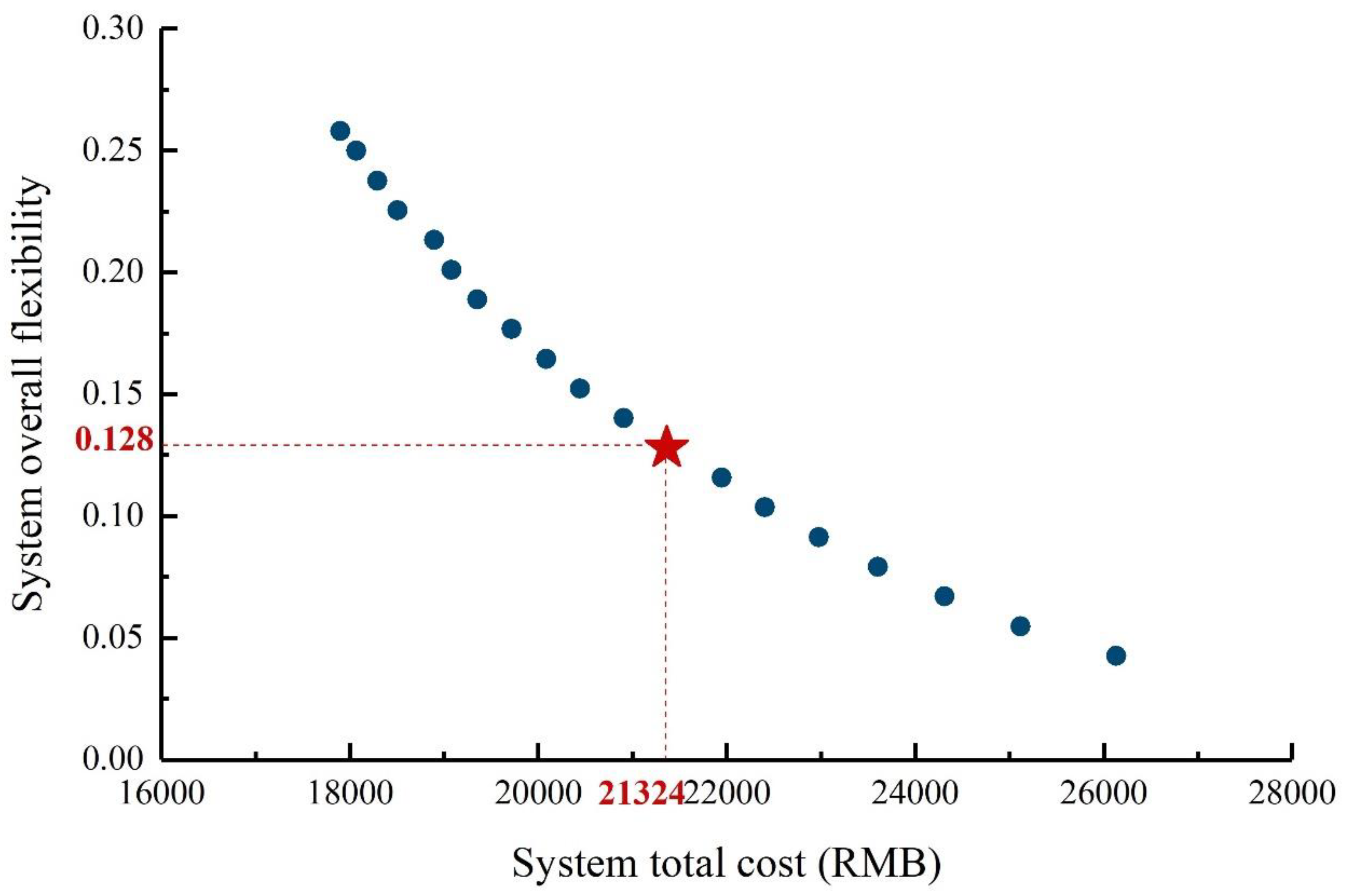
Based on the analysis of the previous section’s results, optimizing the system cost often restricts flexibility enhancement. Additionally, excessively high renewable energy penetration rates can lead to insufficient flexibility. Conversely, when flexibility is the sole optimization objective, the system incurs prohibitively high costs. These findings highlight an inherent contradiction between improving system flexibility and minimizing economic costs, rendering simultaneous optimization of both aspects challenging. To address this conundrum, this paper employs a multi-objective optimization approach to concurrently optimize the system’s total economic cost and flexibility. This method yields a set of non-dominated solutions within the optimization feasible domain, collectively forming the Pareto front, as illustrated in Figure 13.

As depicted in Figure 13, in the initial segment of the Pareto front (cost range: 18,000–21,000 RMB), a notable increase in system flexibility accompanies the rise in economic cost. During the early stages of flexibility improvement, ample room exists for implementing strategies to enhance flexibility. This can be achieved by expanding the capacity of flexible resource equipment and conducting straightforward system scheduling. In contrast, the latter portion of the Pareto front demonstrates a gradual deceleration in the rate of flexibility improvement, an escalating cost burden for further enhancements, and an increasing difficulty in augmenting system flexibility.

Utilizing a fuzzy decision-making method, an optimal compromise solution is identified on the Pareto front, marked by the red star in Figure 13. This solution represents the optimal trade-off when considering both economic and flexibility aspects in system optimization, effectively satisfying the dual optimization requirements of economy and flexibility. Notably, this solution is situated near the inflection point of the trend observed in the previous analysis, aligning well with the overall system behavior.

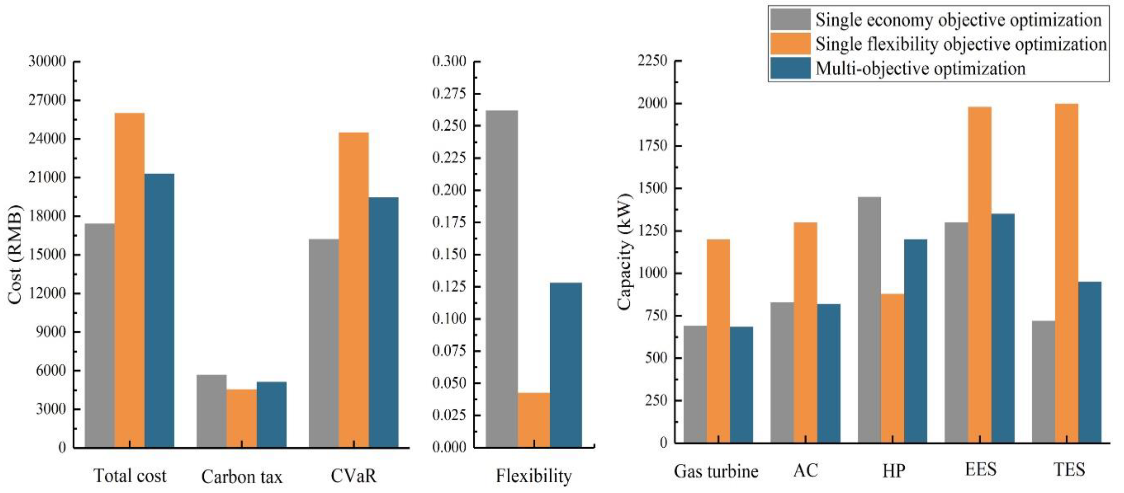
Figure 14 presents the results of multi-objective optimization regarding cost, flexibility, and the capacity of each piece of equipment. When compared with the outcomes of the two single-objective optimizations, it is evident that the trends in system carbon tax, CVaR, and capacity mirror those of cost and flexibility. Multi-objective optimization not only achieves economic efficiency but also enhances system flexibility. Calculation of the risk factors under the three optimization scenarios reveals that the risk factor for multi-objective optimization is 0.91, which is lower than 0.93 under single economy objective optimization and 0.94 under single flexibility objective optimization. This indicates that multi-objective optimization not only improves system flexibility but also reduces system risk and enhances overall system security.

Regarding system equipment capacity, there is a slight upward trend compared to the results of single economy objective optimization. This suggests that increasing system capacity to improve flexibility is a relatively straightforward approach, albeit associated with higher costs. A more cost-effective strategy involves fine-tuning equipment capacity and focusing on optimizing operation scheduling to enhance flexibility. This finding underscores the importance of considering real-world conditions and environmental factors during actual system design and operation, and of implementing appropriate measures to improve flexibility in a balanced manner.

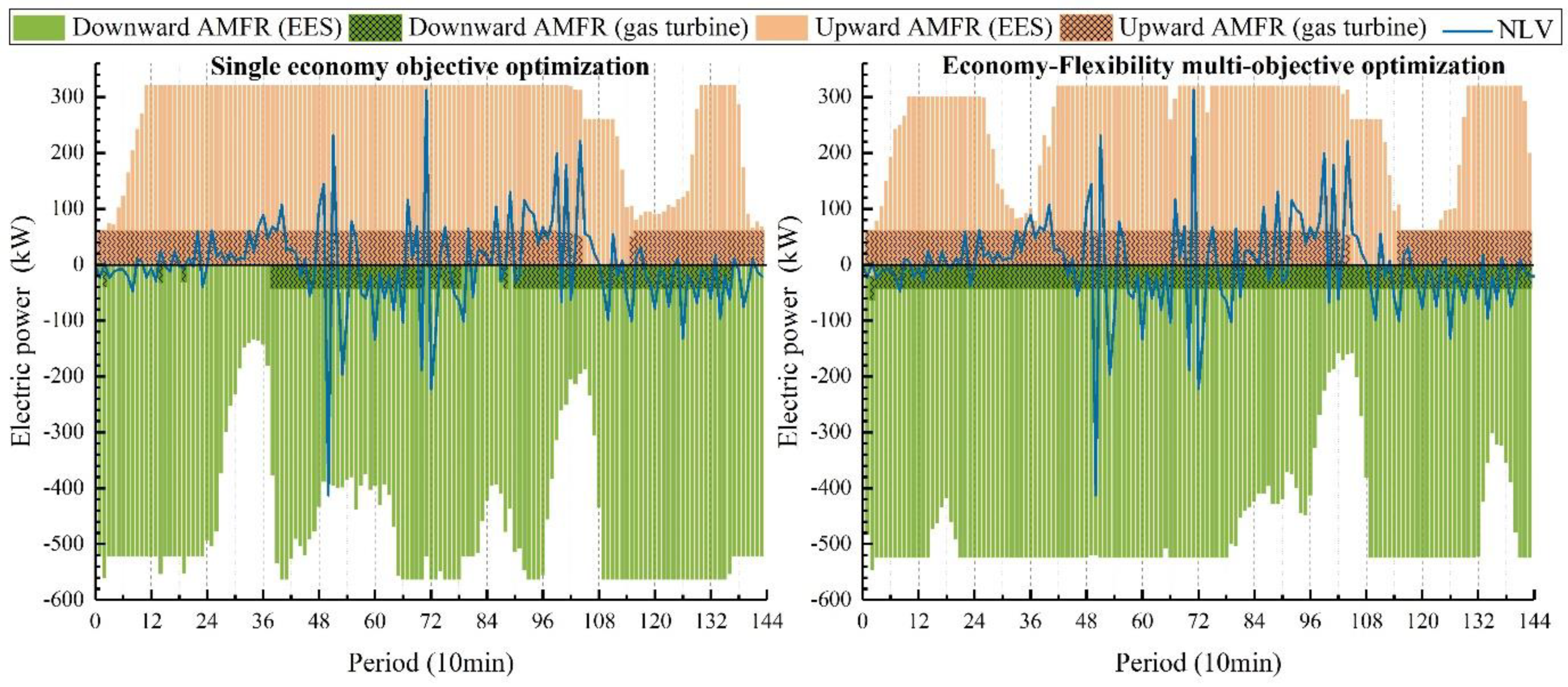
Figure 15 compares the upward/downward AMFR and NLV under the three optimization objectives. The results demonstrate that multi-objective optimization can effectively alleviate the downward flexibility constraints under single economy objective optimization and the flexibility limitations under single flexibility objective optimization (highlighted in the red box). This is accomplished through efficient operational adjustments without substantial changes to equipment capacity. Simultaneously, multi-objective optimization reduces the equipment capacity redundancy observed under single flexibility objective optimization, resulting in a more stable supply of system flexible resources, particularly for downward flexibility. However, the multi-objective optimization approach is not without limitations. As evident from the figure, the system still faces constraints in supplying upward flexible resources, especially at the peak of NLV, posing challenges to the absorption of a higher proportion of renewable energy.

To further assess the capability of multi-objective optimization in order to enable the system to accommodate a higher proportion of renewable energy, this paper analyzes the system’s flexibility demand and optimal flexibility supply when the system confronts the NLV corresponding to a 60% renewable energy penetration rate. Given that the upward AMFR after single flexibility objective optimization has already reached the critical threshold of insufficient flexibility at a 50% penetration rate (as shown in Figure 10), it is unable to support the absorption of additional renewable energy. Therefore, a comparison is made only between the results of single economy objective optimization and multi-objective optimization, as illustrated in Figure 16.

As shown in Figure 16, under the NLV of a 60% penetration rate, the downward AMFR of single economy optimization proves inadequate. In contrast, multi-objective optimization maintains a substantial flexible resource margin at the peak of the downward NLV, enabling it to effectively mitigate system fluctuations and risks associated with increased renewable energy integration. At the peak of the upward NLV, multi-objective optimization precisely meets the current flexibility demand. This indicates that multi-objective optimization not only improves economic performance and flexibility but also increases the system’s renewable energy absorption rate by nearly 10%. However, it also highlights the need to further enhance upward flexibility, consistent with the analysis in Section 5.3.

The results of all optimization objective models consistently demonstrate that the Electric Energy Storage (EES) system is the primary provider of flexible resources for the integrated energy system. Its rapid operational response capabilities are crucial for the provision and scheduling of flexible resources. Through collaborative operation with diverse flexible resources and the implementation of intelligent scheduling strategies, a multi-level and multi-time scale flexible supply system can be established. Moreover, in the context of future large-scale energy system development, cross-system interactive dispatching within a region can fully exploit the flexibility advantages of combined energy storage systems.

6. Conclusions

Aiming to enhance the operational flexibility and renewable energy utilization rate of IES amidst multiple complex uncertainties, this paper delves into the research on IES flexibility. Herein, multi-dimensional flexibility evaluation indexes encompassing the “Source–Structure–Demand” aspects of IES are established, and a multi-objective optimization model that accounts for flexibility and uncertainty is constructed. To validate the proposed indexes and the multi-objective optimization method, single economy objective optimization, single flexibility objective optimization, and multi-objective optimization are conducted. Additionally, optimizations under varying renewable energy proportions are performed to elucidate the significance of enhancing IES flexibility. The detailed findings are as follows:

(1)

Results of Single Economy Objective Function Optimization

Under the single economy objective function of minimizing the system’s total cost, the gas turbines and electric energy storage within the IES provide a substantial flexible resource margin. However, the system exhibits a high degree of dependence on the power grid, and the inherent flexibility of the IES itself remains inadequate. These results underscore the necessity of improving the system’s flexibility.

(2)

Results of Single Flexibility Objective Function Optimization

Following the single flexibility objective optimization, the significant and excessive enhancement of flexibility has a pronounced negative impact on the system’s economy and safety. Specifically, the cost and risk increase by nearly 50%, while the effect on carbon emissions is relatively negligible. Regarding the system configuration, there is a notable requirement for expanding the capacity of each piece of equipment in the IES. Nevertheless, after optimization, the flexible resources demonstrate greater stability.

(3)

Results of Flexibility under Different Renewable Energy Penetration Rates

The optimization results under diverse renewable energy penetration rates reveal that an increase in the penetration rate can reduce the IES’s energy consumption costs and carbon emissions. Conversely, this leads to an elevation in IES risk and a decline in IES flexibility. Moreover, with an excessive increase in the penetration rate, the IES encounters insufficient flexibility. This indicates that, in practical applications, it is essential to comprehensively consider the actual conditions of the IES when selecting an appropriate penetration rate.

(4)

Results of Multi-Objective Function Optimization

Under multi-objective optimization, the IES not only maintains economic efficiency but also enhances system flexibility and security through fine-tuning equipment capacity and focusing on optimizing operation scheduling. Additionally, the flexible resources available through multi-objective optimization are more abundant, and this approach increases the system’s renewable energy absorption rate by nearly 10%. These results fully demonstrate the importance of conducting multi-objective optimization of IES while considering flexibility under complex uncertain conditions.

The flexibility evaluation system and multi-objective optimization model for IES under uncertainties established in this paper possess universality and versatility. They offer a more realistic and robust approach to the collaborative optimization of IES, especially in the context of the growing integration of renewable energy. The evaluation and optimization of flexibility can effectively enhance the system’s capability to handle uncertain disturbances while maintaining low-carbon operation. This study not only deepens the theoretical understanding of flexibility in IES but also provides practical tools for enhancing system resilience and efficiency during the energy transformation process.

Notably, the model in this paper emphasizes the representation of the design-state operation to enhance universality. In practical scenarios, however, equipment does not always operate under designed conditions. Off-design operation situations may occur, resulting in discrepancies between the actual operation and the optimization results. This limitation presents an area for improvement in future research. To meet the requirements of real-time flexible operation scheduling, incorporating off-design characteristic models of system operation can achieve comprehensive coverage of operating conditions.

Looking ahead, future IES design and operation should prioritize the application of advanced multi-objective optimization methods, such as dynamically adjusting the weights of each objective to achieve refined optimization. Attention should also be paid to the precise allocation of flexible resources and the pivotal role of the energy storage system. Finally, by leveraging the coordinated progress of policy support and market mechanisms, and by fully utilizing demand response and cross-system coordinated interactions within the region for joint energy storage, the sustainable development of IES can be effectively promoted.