Optimal Operation of a Two-Level Game for Community Integrated Energy Systems Considering Integrated Demand Response and Carbon Trading

Abstract

In light of the current challenges posed by complex multi-agent interactions and competing interests in integrated energy systems, an economic optimization operation model is proposed. This model is based on a two-layer game comprising a one-master–many-slave structure consisting of an energy retailer, energy suppliers, and a user aggregator. Additionally, it considers energy suppliers to be engaged in a non-cooperative game. The model also incorporates a carbon trading mechanism between the energy retailer and energy suppliers, considers integrated demand response at the user level, and categorizes users in the community according to their energy use characteristics. Finally, the improved differential evolutionary algorithm combined with the CPLEX solver (v12.6) is used to solve the proposed model. The effectiveness of the proposed model in enhancing the benefits of each agent as well as reducing carbon emissions is verified through example analyses. The results demonstrate that the implementation of non-cooperative game strategies among ESs can enhance the profitability of ES1 and ES2 by 27.83% and 18.67%, respectively. Furthermore, the implementation of user classification can enhance user-level benefits by up to 39.51%.

1. Introduction

The considerable rise in greenhouse gas emissions has had a profound impact on the economic development of countries across the globe, with climate change emerging as a significant challenge to global economic growth [1]. The introduction of carbon peaking and carbon neutrality goals has precipitated an urgent need in China to implement an energy transition and construct a new-generation system that is environmentally friendly, low-carbon, secure, and efficient [2]. In this context, integrated energy systems (IESs) that are capable of multi-energy coupling have become the primary means of achieving efficient and clean energy utilization [3,4]. These systems have the potential to dismantle the silos between disparate energy sources, improve energy efficiency, and enhance renewable energy absorption, thereby playing a pivotal role in attaining carbon neutrality and peak carbon goals [5,6].

In the current optimal scheduling of IES, it is recommended that demand response (DR) [7] and the carbon trading mechanism (CTM) [8] be taken into consideration. The implementation of incentive compensation or price changes has the potential to impact energy consumption behavior, optimize the match between supply and demand, and improve system stability through the use of DR mechanisms. As IES is capable of coupling multiple energy sources, integrated demand response (IDR), which encompasses electric, gas, heat, and cold loads, is gradually replacing the conventional approach of DR for electric loads [9,10]. In a community-integrated energy system (CIES) model, Wang et al. [11] investigated the potential use of DR with electric–thermal synergy to reduce costs and carbon emissions. Their findings suggest that DR with electric–thermal synergy may be an effective strategy for achieving these environmental and economic goals. Liang et al. [12] introduced the idea of IDR in the optimal allocation of energy storage in IES. They then proceeded to verify the effectiveness of IDR in optimizing energy storage allocation as well as cost reduction. Wang et al. [13] developed a multi-objective optimization model of IES that considers IDR, thereby further exploiting the energy consumption potential on the demand side. On the other hand, the CTM represents an efficacious method for regulating carbon emissions through the utilization of market mechanisms. A substantial corpus of research has been undertaken with the objective of integrating the CTM into the economic optimization of IES. So as to achieve a further reduction in the level of carbon emissions within the system, Zhou et al. [14,15] proposed the establishment of a carbon trading market in IES. Chen et al. [16] introduced a price-based CTM model in IES, and the results demonstrate that power scheduling tends to result in a lower level of carbonization compared to scheduling in traditional IES. Ma et al. [5] developed an optimal scheduling model for IES with coupled electric, heat, gas, and carbon considerations and incorporated the CTM into the model. The simulation verification concluded that the CTM improved the utilization of renewable energy. In a multi-objective optimization model for IES, Pan et al. [17] introduced a stepped CTM, and the results demonstrate that the proposed strategy can decrease carbon emissions effectively. Nevertheless, the above literature on the optimal scheduling of IES only considers IDR or the CTM in isolation, without examining the impact of IDR and CTM co-modeling.

In addition, some studies have introduced both IDR and the CTM into IES. Li et al. [18,19] demonstrated that integrating the synergies between IDR and the CTM in an electrothermal IES can effectively reduce carbon emissions and costs. Chen et al. [20] established a CTM with load-side DR in IES, which proved to be an effective method of reducing carbon emissions and improving economic efficiency. Zeng et al. [21] developed a two-level IES model in which the load-side flexibility of whole-process carbon emissions was considered at a lower level. The incorporation of whole-process carbon emissions and IDR was verified to enhance the economic and low-carbon performance of the system.

Currently, the literature on IES optimal scheduling primarily focuses on the centralized optimization approach. This approach, however, does not fully address the issue of competing interests among the agents within the system. Instead, it primarily considers the maximization of the overall interests of the system. This does not align with the prevailing concept of the regional autonomy of IES [22]. It is recommended that future research concentrate on the distributed optimization of IES in order to satisfy the interests of a variety of agents. In addressing the competing interests of agents in IES distributed optimization, Stackelberg game theory offers an appropriate means of analysis [22,23]. In this context, Zhang et al. [24] established a master–slave game model between the integrated energy system operator (IESO) and each IES. This was performed in order to investigate the pricing strategy of the IESO and the optimization strategy of the IES. Wang et al. [25] constructed a Stackelberg game model to describe the competitive dynamics at play between the three key parties involved in the energy sector: energy suppliers, energy storage operators, and energy users. In order to solve the problem of renewable energy consumption in distributed integrated energy systems (DIES), Wang et al. [26] established a single-master–multiple-slave (SMMS) model based on the Stackelberg game. Wang et al. [27] employed a Stackelberg game to optimize the pricing of energy service providers and the energy use strategies of users, with the objective of achieving the low-carbon and economic goals of the system. Yuan et al. [28] conducted an analysis of the relationship between IES and users, wherein IES, functioning as a leader, employs time-of-use pricing strategies with the objective of enhancing profits and market competitiveness. Li et al. [29] constructed an SMMS model as part of the two-level optimization of IES, with the objective of achieving regional autonomy in IES and balancing the interests of leaders and followers.

Furthermore, research has been conducted that considers IDR and the CTM in the context of competition between agents in the IES. In order to address the discrepancy between the output of renewable energy sources and the demand from users, IDR was considered in the Stackelberg game, as discussed in [30]. Latifi et al. [31] considered DR in the game model of followers to maximize consumer satisfaction. Shen et al. [32] incorporated both IDR and the CTM into a Stackelberg game low-carbon economic dispatch model, with the objective of reducing the system’s carbon emissions and enhancing the user benefits. In a Stackelberg game, Yan et al. [33] introduced an IDR model that considered the psychological aspects of consumers. Their findings demonstrate that an IDR that incorporates consumer psychology can markedly enhance consumer surplus. Qin et al. [34] introduced both IDR and the CTM into the game model of a CIES, considering IDR and the CTM on the user level and the CTM on the supply level. Hou et al. [35] proposed the use of the CTM in IES as a means of achieving low-carbon operation in the system. Meanwhile, a game is undertaken between the IESO and the users, who participate in the IDR based on the energy price set by the IESO to enhance their own benefits.

Most studies have focused on vertical supply–demand multi-agent master–slave games, with limited research into multi-agent games at the same level. This paper constructs a non-cooperative game model for energy suppliers on the supply side, which facilitates multi-agent collaborative optimization and development. The existing studies generally categorize demand-side users into a single group, assuming that users have identical energy consumption preferences. However, in reality, users exhibit significant differences in their energy consumption preferences, and these variations can influence the equilibrium outcomes of demand-side games within integrated energy systems. This paper categorizes demand-side users into four groups based on their energy consumption characteristics. Each category of users participates in a demand response based on their own energy consumption preferences, achieving load reduction and transfer within the system while enhancing their own energy consumption satisfaction.

Although some studies have used the Stackelberg game to address the internal supply and demand relationships, there is still room for improvement. Firstly, in the contemporary energy market, where competition from numerous ESs is a prominent feature, the traditional approach of focusing solely on the game between supply and demand is no longer sufficient to meet the optimization requirements of modern DIES. Secondly, there are few studies that have introduced both IDR and the CTM into the Stackelberg game, and considering either IDR or the CTM in isolation is insufficient to meet the low carbon needs of today’s IES. Finally, there is considerable variation in the energy use preferences of users. However, the aforementioned studies tend to assume that these preferences are homogeneous, which is not realistic.

In light of the aforementioned analyses, the objective of this paper is to put forth a two-level game model for CIES that considers IDR and the CTM. The energy retailer (ER) is introduced as the manager of the CIES, while energy suppliers (ESs) and user aggregators are introduced as the followers, forming an SMMS game relationship. In addition, a non-cooperative game relationship is established among the ESs. Moreover, the model incorporates considerations of user-side diversity through the classification of community users according to their energy-use characteristics. This paper introduces an improved differential evolution algorithm, which is designed to enhance the speed and accuracy of model optimization in high-dimensional and nonlinear two-level master–slave game models. The proposed algorithm incorporates the double mutation strategy and adaptive crossover strategy into the traditional differential evolution algorithm to achieve this objective. Subsequently, the efficacy of the aforementioned model and algorithm is validated through the utilization of illustrative simulations. The principal contributions of this paper are as follows:

(1)

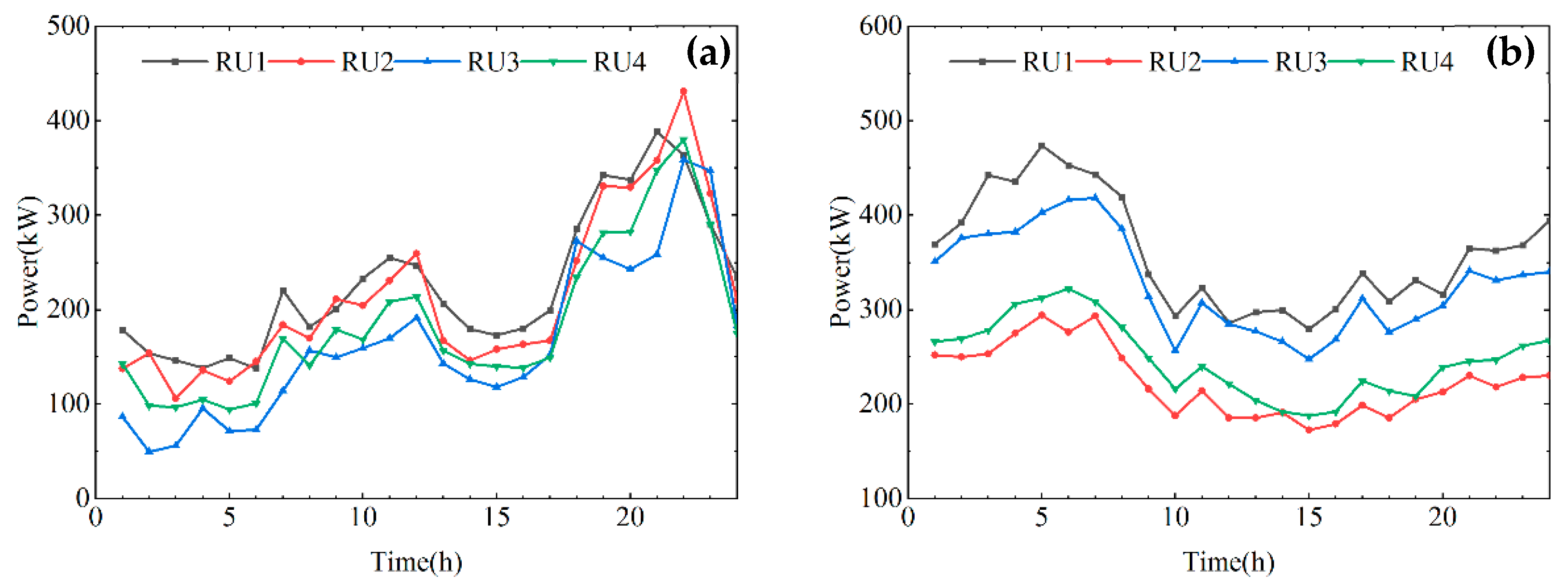
A segmentation of users on the basis of their energy-use characteristics is conducted, and the results demonstrate that this segmentation allows user aggregators to more effectively participate in the demand–response market and improve user-side benefits.

(2)

A two-level game optimization model is proposed, wherein the ER, acting as a leader, forms an SMMS model with the ESs and a user aggregator, who are designated as followers. Non-cooperative games are established among the follower ESs, coordinating the interests of each ES. Additionally, to increase user benefits and reduce system carbon emissions, IDR and the CTM are introduced into the two-level game optimization model.

(3)

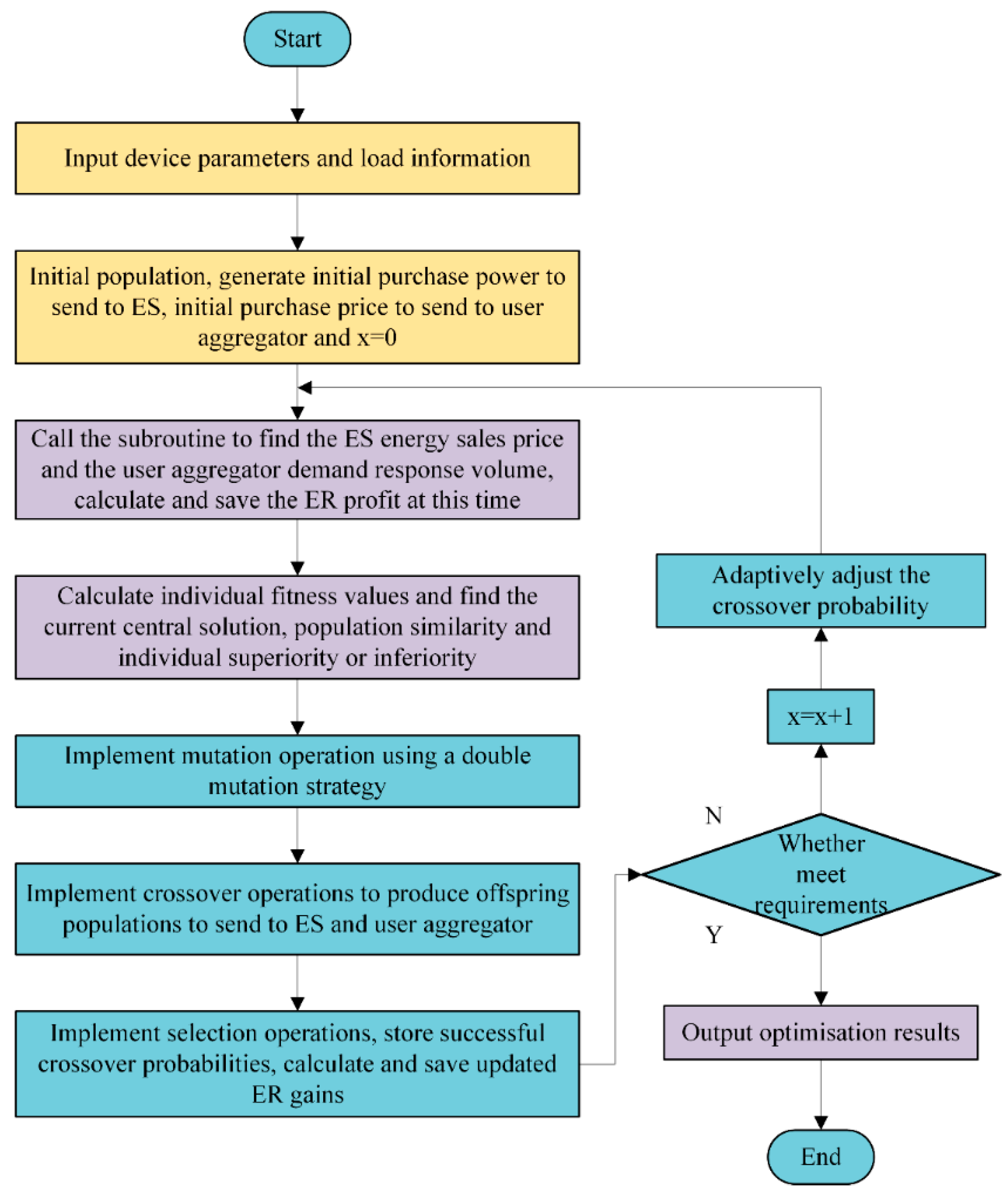
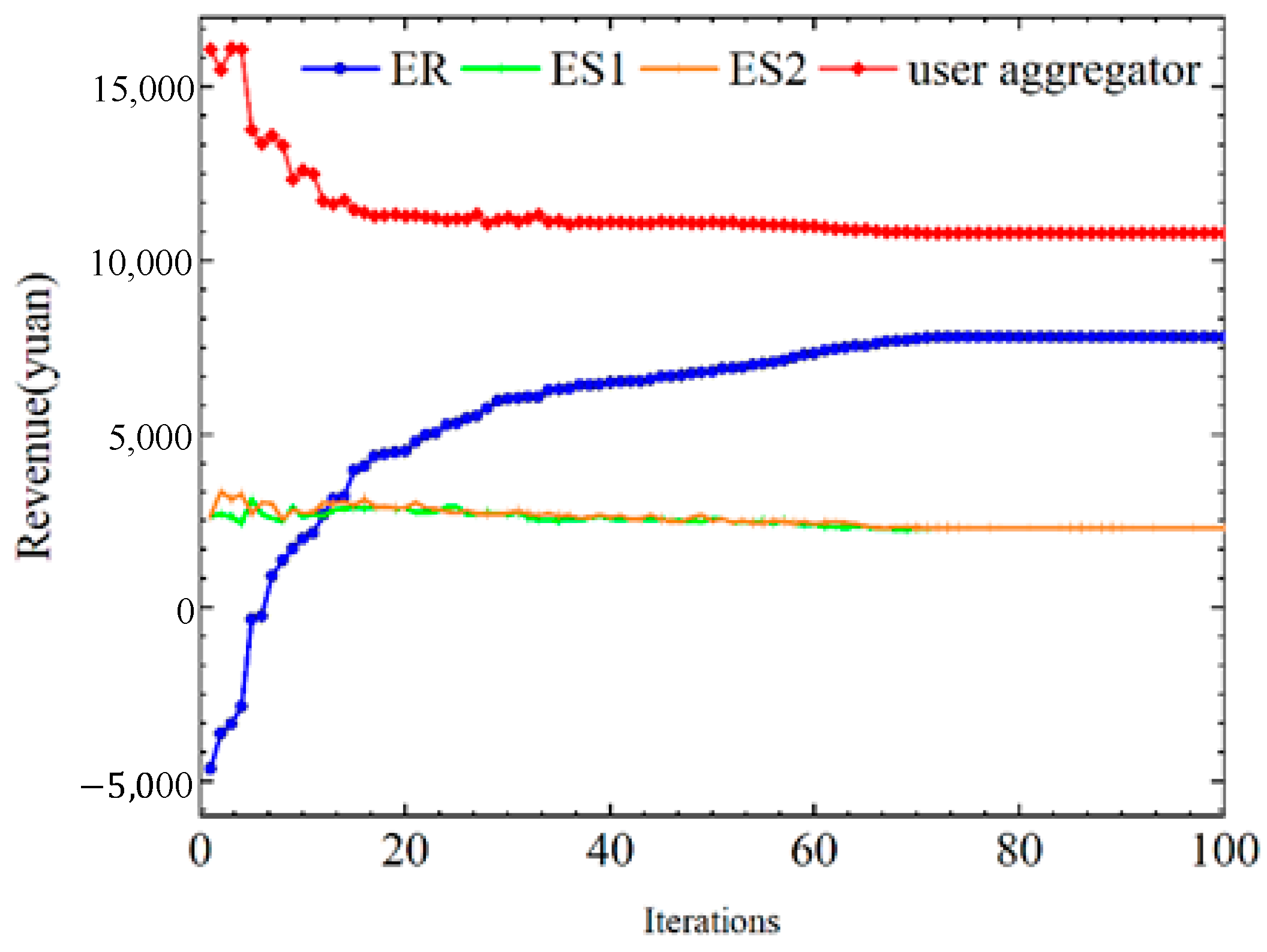
To assess the formulated model, an improved differential evolutionary algorithm is employed in collaboration with the CPLEX solver (v12.6). The case study verifies the convergence of the algorithm and the efficacy of the strategy proposed in this paper in considering the benefits of the various agents while reducing carbon emissions.

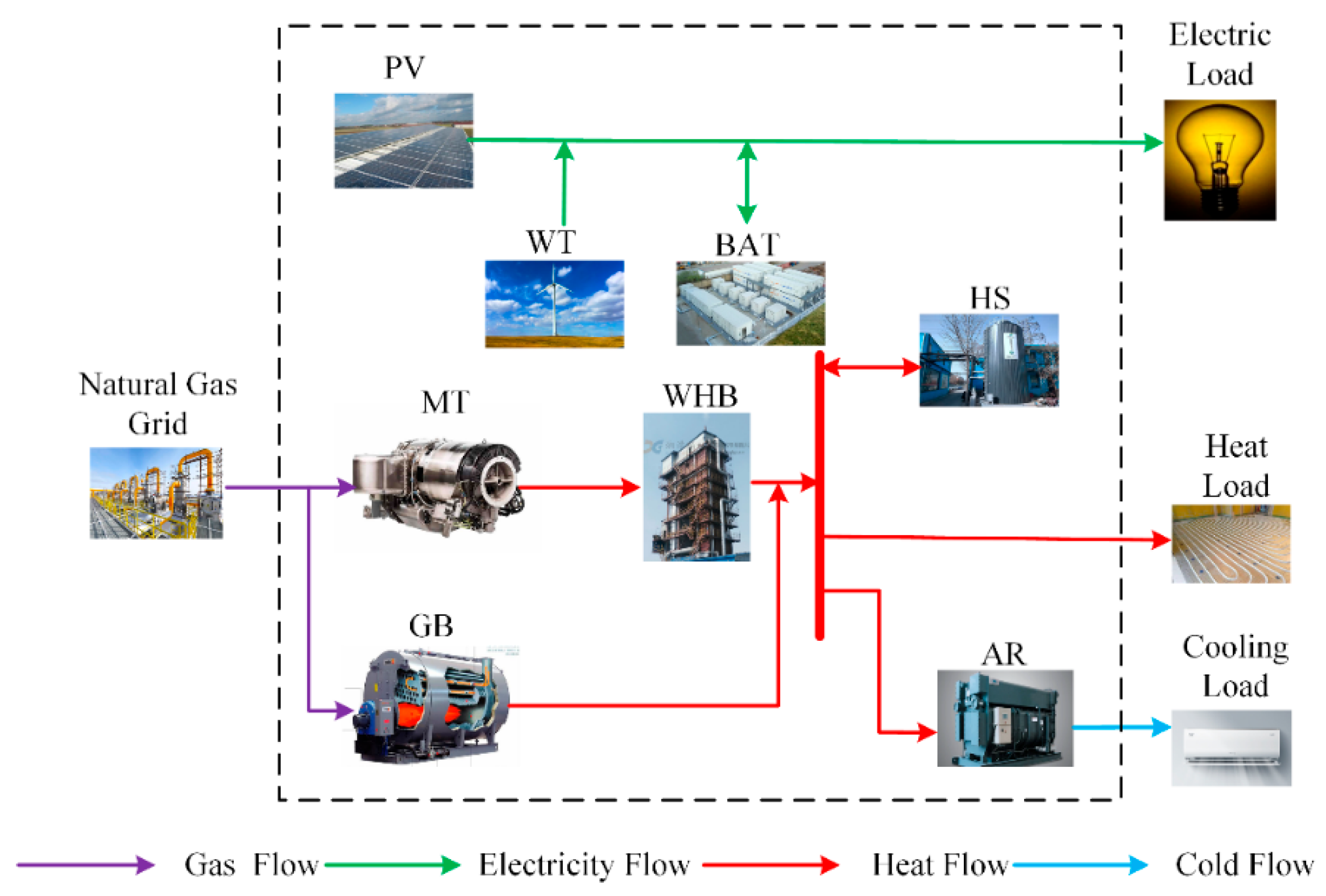
The rest of this paper is organized as follows: Section 2 outlines the structure of the CIES. Section 3 provides a detailed description of the CIES optimization model, which accounts for both IDR and the CTM. Section 4 proposes a two-level game model for analyzing the operational strategies of each agent. Section 5 describes the process of solving the model. Section 6 discusses and analyzes the results through a case study. Finally, Section 7 offers a conclusion to the paper.

2. CIES Structure

The CIES proposed in this paper is composed of an ER, two ESs, and a user aggregator. An ER is a bridge between supply and demand, navigating the competing interests of the system’s primary stakeholders and facilitating the rational scheduling of energy to achieve equilibrium between supply and demand. The CIES structure is illustrated in Figure 1.

The use of big data and forecasting technology by ER enables the initial load of the customer to be predicted. Subsequently, the price at which energy is sold to the users and the energy purchasing power of ESs are set based on the ESs’ historical energy prices and the electricity and heat prices of the power grid and heat company. This approach allows the ER to optimize its own benefits. The objective of the user aggregator is to optimize the benefits derived by the user community by optimizing load purchase volumes. The ES provides energy for the CIES, comprising combined cooling heating and power (CCHP) units that primarily achieve this objective by optimizing their own energy sales prices and unit output.

The energy trading process, as previously outlined, comprises two distinct phases: the initial decision-making phase, occurring at the highest levels of the organizational structure, and the subsequent response phase, occurring at the lowest levels. The initial phase involves the upper-layer ER in the formulation of an energy sales price and purchase power strategy, which is based on the load demand and historical selling price information of the ESs. In the initial phase, the ER establishes the energy sales price and energy power purchase strategy, basing these decisions on load demand and historical selling price information derived from the ESs. In the subsequent phase, the lower-layer ESs and user aggregator determine the energy sales price and load demand response quantity, respectively, based on the ER’s decision. Concurrently, the ER initiates a new round of decision-making based on the lower layer’s strategy.

3. The CIES Optimization Model Considering Both IDR and CTM

3.1. Modeling of New Energy CCHP

The variables and abbreviations introduced in this paper are shown in

Table 1. Variables and abbreviations.

Variables and Abbreviations	Specific Meaning	Variables and Abbreviations	Specific Meaning
IES	integrated energy systems	$D_{ER}$ , $D_{ES,i}$	the carbon allowances of ER and ESi
DR	demand response	$P_{buy}\left(t\right)$ , $H_{buy}\left(t\right)$	the purchasing of electricity and heat by ER
CTM	carbon trading mechanisms	${\theta }_e$ , ${\theta }_h$	the carbon emission allowances per unit of electricity and heat
IESO	integrated energy system operator	$E_{ER}$ , $E_{ES,i}$	the actual carbon emissions of ER and ESi
SMMS	single-master–multiple-slave	$P_{gtr,i}\left(t\right)$	the sum of MT and GB output power of ESi
ER	energy retailer	$a_1$ , $b_1$ , $c_1$ , $a_2$ , $b_2$ , $c_2$	the carbon emission calculation factors for coal and natural gas-fired energy plants
ESs	energy suppliers	$F_{C{O}_2}$	the carbon trading cost
CIES	community integrated energy system	$F_{ER}$	the overall revenue of ER in a single day
CCHP	cooling, heating, and power	$f_{sell}\left(t\right)$	the revenue of supplying energy to users
PV	photovoltaics	$C_{ES}\left(t\right)$	the cost of purchasing energy from ESs
WT	wind turbine	$C_{grid}\left(t\right)$ , $C_h\left(t\right)$	the cost of purchasing electricity and heat
BAT	storage batteries	$P_{ue,k}\left(t\right)$ , $P_{uh,k}\left(t\right)$	the demand for electricity and heat load of the kth class of users
MT	micro gas turbine	${\rho }_{es}\left(t\right)$ , ${\rho }_{hs}\left(t\right)$	ER’s electricity and heat prices
WHB	waste heat boiler	$P_{e.i}\left(t\right)$ , $P_{h.i}\left(t\right)$	ER’s electricity and heat power purchased from ESi
AR	absorption refrigerator	${\rho }_{eb,i}\left(t\right)$ , ${\rho }_{hb,i}\left(t\right)$	the electricity and heat selling price of ESi
GB	gas boiler	${\rho }_{\mathrm{e}}\left(t\right)$ , ${\rho }_{\mathrm{h}}\left(t\right)$	the electricity and heat price from the higher level purchased by ER
HS	heat storage	$F_{ES,i}$	the overall revenue of ESi
$H_{MT,i}\left(t\right)$	residual heat generated by MT of ESi	$C_{gas,i}\left(t\right)$	the fuel cost incurred by the MT and GB of ESi
$P_{MT,i}\left(t\right)$	the output power of MT of ESi	$C_{om,i}\left(t\right)$	the operation and maintenance costs for equipment of ESi
${\eta }_{MT,i}$ , ${\gamma }_{MT,i}$	generating efficiency and heat loss factor of MT in ESi	$C_{es,i}\left(t\right)$	the energy storage unit operation and maintenance costs of ESi
$H_{WHB,i}\left(t\right)$	the output thermal power of WHB	$a_{be,i}\left(t\right)$ , $a_{bh,i}\left(t\right)$	the base electricity and heat prices of ESi
${\eta }_{WHB,i}$	the heat recovery efficiency of WHB	$b_{fe,i}$ , $b_{fh,i}$	the coefficients of fluctuation of electricity and heat prices for ESi
$H_{AR,i}\left(t\right)$	the refrigeration power of AR of ESi	$U_{user}\left(t\right)$	the user’s energy utility
${\eta }_{\mathrm{AR},\mathrm{i}}$	the refrigeration efficiency of AR of ESi.	${\alpha }_{e,k}$ , ${\beta }_{e,k}$ , ${\alpha }_{h,k}$ , ${\beta }_{h,k}$	the preference coefficients for electricity and heat

. The structure of the CCHP in this paper is illustrated in Figure 2. The main devices included in the system are photovoltaics (PV), a wind turbine (WT), storage batteries (BAT), a micro gas turbine (MT), a waste heat boiler (WHB), an absorption refrigerator (AR), a gas boiler (GB), and heat storage (HS).

The MT will generate excess heat while generating electricity, which can be recovered and processed by the WHB. This heat can then be used for cooling by absorption chillers or directly for heating. The recovery process can be expressed as follows:

$$H_{MT,i}\left(t\right)={\displaystyle \frac{1-{\eta }_{MT,i}-{\gamma }_{MT,i}}{{\eta }_{MT,i}}}{P}_{MT,i}\left(t\right)$$

(1)

$$H_{WHB,i}\left(t\right)=H_{MT,i}\left(t\right){\eta }_{WHB,i}$$

(2)

$$H_{AR,i}\left(t\right)=\left[H_{WHB,i}\left(t\right)+H_{GB,i}\left(t\right)\right]{\eta }_{AR,i}$$

(3)

where $H_{MT,i}\left(t\right)$ denotes the residual heat generated by the MT of ESi in period t; $P_{MT,i}\left(t\right)$ represents the output power of the MT of ESi in period t; ${\eta }_{MT,i}$ and ${\gamma }_{MT,i}$ represent the generating efficiency and heat loss factor of the MT in ESi, respectively; $H_{WHB,i}\left(t\right)$ denotes the output thermal power of the WHB of ESi in period t; ${\eta }_{WHB,i}$ represents the heat recovery efficiency of the WHB of ESi; $H_{AR,i}\left(t\right)$ represents the refrigeration power of the AR of ESi in period t; and ${\eta }_{\mathit{AR},i}$ represents the refrigeration efficiency of the AR of ESi.

During the operation of the equipment, the maximum and minimum bounds of the output power and climb rate must be satisfied.

$$P_{\varpi ,\mathrm{i},\min }\le P_{\varpi ,\mathrm{i}}\left(t\right)\le P_{\varpi ,\mathrm{i},\max }$$

(4)

$$r_{\varpi ,\mathrm{i}}^d\le P_{\varpi ,\mathrm{i}}\left(t\right)-P_{\varpi ,\mathrm{i}}\left(t-1\right)\le r_{\varpi ,\mathrm{i}}^u$$

(5)

where $\varpi \in \left\{PV,WT,BAT,MT,WHB,GB,HS\right\}$; $P_{\varpi ,i}\left(t\right)$ denotes the output power of equipment $\varpi$ of ESi in period t; $P_{\varpi ,i,\max }$ and $P_{\varpi ,i,\min }$ represent the maximum and minimum bounds of output power of equipment $\varpi$ of ESi, respectively; and $r_{\varpi ,\mathrm{i}}^u$ and $r_{\varpi ,\mathrm{i}}^d$ represent the up and down ramping limits of equipment $\varpi$ of ESi, respectively.

In this paper, the models of power and heat storage equipment are similar, so the power storage and heat storage devices are modeled uniformly, i.e.,

$$Q_i^x\left(t\right)=Q_i^x\left(t-1\right)\left(1-v_i^x\right)+P_{char,i}^x\left(t\right){\eta }_{char,i}^x-{\displaystyle \frac{P_{dis,i}^x\left(t\right)}{{\eta }_{dis,i}^x\left(t\right)}}$$

(6)

$$Q_{i,\min }^x\le Q_i^x\left(t\right)\le Q_{i,\max }^x$$

(7)

$$Q_i^x\left(1\right)=Q_i^x\left(24\right)$$

(8)

$$0\le P_{char,i}^x\left(t\right)\le P_{char,i,\max }^x{S}_{char,i}^x\left(t\right)$$

(9)

$$0\le P_{dis,i}^x\left(t\right)\le P_{dis,i,\max }^x{S}_{dis,i}^x\left(t\right)$$

(10)

$$S_{char,i}^x\left(t\right)+S_{dis,i}^x\left(t\right)\le 1$$

(11)

where x denotes the index of the energy storage device, with $x=1~2$ for BAT and HS, respectively; $Q_i^x\left(t\right)$ denotes the energy stored in the energy storage equipment of ESi in period t; $Q_{i,\max }^x$ and $Q_{i,\min }^x$ represent the maximum and minimum stored energy bounds of the energy storage device of ESi, respectively; $Q_i^x\left(1\right)$ and $Q_i^x\left(24\right)$ represent the stored energy in energy storage device of ESi at the start and finish of the day, respectively; $P_{char,i}^x\left(t\right)$ and $P_{dis,i}^x\left(t\right)$ represent the charging and discharging power of the energy storage device of ESi in period t, respectively; $P_{char,i,\max }^x$ and $P_{dis,i,\max }^x$ represent the upper power limits of ESi’s energy storage device during charging and discharging processes, respectively; $v_i^x$ represents the energy dissipation coefficient of ESi; ${\eta }_{char,i}^x$ and ${\eta }_{dis,i}^x\left(t\right)$ represent the efficiency of the charging and discharging processes of ESi, respectively; and $S_{char,i}^x\left(t\right)$ and $S_{dis,i}^x\left(t\right)$ are 0–1 variables, the values of which are 1 when the device is running and 0 when the equipment stops, to ensure that the energy storage equipment is not engaged in the charging and discharging of energy simultaneously.

3.2. Modeling of CTM

The fundamental premise of the CTM is to regulate carbon emissions by establishing legally binding carbon emission rights, which are then traded as commodities [36]. If the actual carbon emissions are less than the carbon allowances, excess allowances can be traded for revenue on carbon trading markets; conversely, carbon allowances must be purchased from the carbon market.

This paper adopts the method of unpaid carbon allowance allocation, in which the system receives unpaid carbon allowances for electricity and thermal power purchased from the upper level, MT, and GB. The formula for calculating carbon allowances for the system is expressed as

$$D_{ER}={\theta }_e{\displaystyle \sum _{t=1}^T{P}_{buy}\left(t\right)}+{\theta }_h{\displaystyle \sum _{t=1}^T{H}_{buy}\left(t\right)}$$

(12)

$$D_{ES,i}={\theta }_h{\displaystyle \sum _{t=1}^T\left[\phi P_{MT,i}\left(t\right)+H_{MT,i}\left(t\right)+H_{GB,i}\left(t\right)\right]}$$

(13)

where T denotes a dispatch cycle; $D_{ER}$ and $D_{ES,i}$ represent the carbon allowances of ER and ESi, respectively; $P_{buy}\left(t\right)$ and $H_{buy}\left(t\right)$ denote the purchasing of the electricity and heat of ER from the higher level in period t, respectively; ${\theta }_e$ and ${\theta }_h$ represent the carbon emission allowances per unit of electricity and heat, respectively; and $\phi$ is the electricity transfer efficiency, which is 1.9.

The formula for the calculation of the actual carbon emissions for each agent is expressed as

$$E_{ER}={\displaystyle \sum _{t=1}^T\left\{a_1\left[P_{buy}^2\left(t\right)+H_{buy}^2\left(t\right)\right]+b_1\left[P_{buy}\left(t\right)+H_{buy}\left(t\right)\right]+2c_1\right\}}$$

(14)

$$P_{gtr,i}\left(t\right)=P_{MT,i}\left(t\right)+H_{MT,i}\left(t\right)+H_{GB,i}\left(t\right)$$

(15)

$$E_{ES,i}={\displaystyle \sum _{t=1}^T\left[a_2{P}_{gtr,i}^2\left(t\right)+b_2{P}_{gtr,i}\left(t\right)+c_2\right]}$$

(16)

where $E_{ER}$ and $E_{ES,i}$ represent the actual carbon emissions of ER and ESi, respectively; $P_{gtr,i}\left(t\right)$ represents the sum of power output from the MT and GB of ESi in period t; $a_1$, $b_1$, $c_1$ and $a_2$, $b_2$, $c_2$ represent the carbon emission factors used in calculations pertaining to coal and natural gas-fired energy plants, respectively.

The present paper considers a laddered CTM, which entails the establishment of a laddered carbon price that rises in accordance with the magnitude of carbon emissions. The equation for calculating the carbon trading cost is expressed as

$$E^{tr}=E-D$$

(17)

$$F_{c{o}_2}=\left\{\begin{array}{ll}\psi E^{tr}& E\le l\\ \psi \left(1+\epsilon \right)\left(E^{tr}-l\right)+\lambda l& 2l\le E\le 2l\\ \psi \left(1+2\epsilon \right)\left(E^{tr}-2l\right)+\lambda \left(2+\epsilon \right)l& 2l\le E\le 3l\\ \psi \left(1+3\epsilon \right)\left(E^{tr}-3l\right)+\lambda \left(3+3\epsilon \right)l& 3l\le E\le 4l\\ \psi \left(1+4\epsilon \right)\left(E^{tr}-4l\right)+\lambda \left(4+6\epsilon \right)l& 4l\le E\end{array}\right.$$

(18)

where $F_{C{O}_2}$ denotes the carbon trading cost; $\psi$ represents the carbon trading price [37]; l represents the length of the carbon emission interval; $\epsilon$ represents the growth factor; $E^{tr}$ represents the carbon emissions trading volume; and D represents the carbon allowances; and E represents the actual carbon emissions.

3.3. Modeling the Benefits of Each Agent

3.3.1. Energy Retailer

The objective of the ER is to maximize revenue by optimizing the price at which energy is purchased and sold. The costs incurred by the ER include the cost of purchasing energy from the ES side, the cost of purchasing electricity from the power grid, and the cost of purchasing heat from the heat company. The process by which the ER maximizes its benefits can be described as follows:

$$\max F_{ER}={\displaystyle \sum _{t=1}^T\left[f_{sell}\left(t\right)-C_{ES}\left(t\right)-C_{grid}\left(t\right)-C_h\left(t\right)-F_{C{O}_2}^{ER}\left(t\right)\right]}$$

(19)

where $F_{ER}$ denotes the overall revenue of the ER in a single day; $f_{sell}\left(t\right)$ represents the revenue of supplying energy to users; $C_{ES}\left(t\right)$ represents the cost of purchasing energy from ESs; and $C_{grid}\left(t\right)$ and $C_h\left(t\right)$ represent the cost of purchasing electricity and heat from the upper level, respectively. The equations for $I_{sell}\left(t\right)$, $C_{ES}\left(t\right)$, $C_{grid}\left(t\right)$, and $C_h\left(t\right)$ are expressed as

$$f_{sell}\left(t\right)={\displaystyle \sum _{k=1}^4\left(P_{ue,k}\left(t\right){\rho }_{es}\left(t\right)+P_{uh,k}\left(t\right){\rho }_{hs}\left(t\right)\right)}$$

(20)

$$C_{ES}\left(t\right)={\displaystyle \sum _{i=1}^n\left(P_{e.i}\left(t\right){\rho }_{eb,i}\left(t\right)+P_{h.i}\left(t\right){\rho }_{hb,i}\left(t\right)\right)}$$

(21)

$$C_{grid}\left(t\right)=\left({\displaystyle \sum _{k=1}^4{P}_{ue,k}\left(t\right)}-{\displaystyle \sum _{i=1}^n{P}_{e,i}\left(t\right)}\right){\rho }_e\left(t\right)$$

(22)

$$C_h\left(t\right)=\left({\displaystyle \sum _{k=1}^4{P}_{uh,k}\left(t\right)}-{\displaystyle \sum _{i=1}^n{P}_{h,i}\left(t\right)}\right){\rho }_h\left(t\right)$$

(23)

where $P_{ue,k}\left(t\right)$ and $P_{uh,k}\left(t\right)$ denote the demand for electricity and the heat load of the kth class of users in period t, respectively; ${\rho }_{es}\left(t\right)$ and ${\rho }_{hs}\left(t\right)$ denote the prices of electricity and heat sold by the ER to users in period t, respectively; $P_{e.i}\left(t\right)$ and $P_{h.i}\left(t\right)$ represent the ER’s electricity and heat power purchased from ESi in period t, respectively; ${\rho }_{eb,i}\left(t\right)$ and ${\rho }_{hb,i}\left(t\right)$ represent the prices at which electricity and heat are sold by ESi in period t, respectively; and ${\rho }_{\mathrm{e}}\left(t\right)$ and ${\rho }_{\mathrm{h}}\left(t\right)$ represent the prices of electricity and heat purchased from the higher level by the ER in period t, respectively.

In order to avoid the ER setting the maximum prices for an extended period of time, it is vital to ensure that the ER’s electricity and heat selling prices are met.

$${\rho }_{\mathrm{g}}\left(t\right)<{\rho }_{\mathrm{es}}\left(t\right)<{\rho }_{\mathrm{e}}\left(t\right)$$

(24)

$${\rho }_{h,\min }\left(t\right)<{\rho }_{hs}\left(t\right)<{\rho }_{h,\max }\left(t\right)$$

(25)

where ${\rho }_{\mathrm{g}}\left(t\right)$ represents the feed-in tariff in period t; and ${\rho }_{h,\min }\left(t\right)$ and ${\rho }_{h,\max }\left(t\right)$ represent the maximum and minimum heat prices in period t, respectively.

Concurrently, the ER is precluded from establishing the maximum price for an extended period, and the ER’s electricity and heat selling prices must be fulfilled.

$${\displaystyle \sum _{t=1}^T{\rho }_{es}\left(t\right)}\le T\overline{{\rho }_e^{\max }}$$

(26)

$${\displaystyle \sum _{t=1}^T{\rho }_{hs}\left(t\right)}\le T\overline{{\rho }_h^{\max }}$$

(27)

where $\overline{{\rho }_e^{\max }}$ and $\overline{{\rho }_h^{\max }}$ denote the highest average price of electricity and heat, respectively.

Concurrently, to guarantee the uninterrupted and secure fulfillment of the user’s energy requirements, the ER procures electric heating power in accordance with the following constraints:

$${\displaystyle \sum _{i=1}^n{P}_{e,i}\left(t\right)}+P_{buy}\left(t\right)={\displaystyle \sum _{k=1}^4{P}_{ue,k}\left(t\right)}$$

(28)

$${\displaystyle \sum _{i=1}^n{P}_{h,i}\left(t\right)}+H_{buy}\left(t\right)={\displaystyle \sum _{k=1}^4{P}_{uh,k}\left(t\right)}$$

(29)

3.3.2. Energy Suppliers

Each ES maximizes its own revenue by optimizing its own energy sales price and equipment output, with each ES’s benefit being the difference between the profit derived from selling energy to the ER and the operating costs. The process by which each ES maximizes its benefits is expressed as

$$\max F_{ES,i}={\displaystyle \sum _{t=1}^T\left(P_{e,i}\left(t\right)c_{eb,i}\left(t\right)+P_{h,i}\left(t\right)c_{hb,i}\left(t\right)-C_{gas,i}\left(t\right)-C_{om,i}\left(t\right)-C_{es,i}\left(t\right)-F_{C{O}_2}^{ES,i}\left(t\right)\right)}$$

(30)

where $F_{ES,i}$ denotes the overall revenue of ESi; $C_{gas,i}\left(t\right)$ represents the fuel cost incurred by the MT and GB of ESi in period t; $C_{om,i}\left(t\right)$ represents the operation and maintenance costs of the equipment of ESi in period t; and $C_{es,i}\left(t\right)$ represents the energy storage unit operation and maintenance costs of ESi in period t.

The relationship between fuel cost and output power for MT and GB can be described in quadratic form as follows [38]:

$$C_{gas,i}\left(t\right)=a_{MT,i}{P}_{MT,i}^2\left(t\right)+b_{MT,i}{P}_{MT,i}^2\left(t\right)+c_{MT,i}+a_{GB,i}{H}_{GB,i}^2\left(t\right)+b_{GB,i}{H}_{GB,i}^2\left(t\right)+c_{GB,i}$$

(31)

where $a_{MT,i}$, $b_{MT,i}$, $c_{MT,i}$ and $a_{GB,i}$, $b_{GB,i}$, $c_{GB,i}$ represent the MT and GB fuel factors for ESi, respectively.

$$C_{om,i}\left(t\right)={\displaystyle \sum _{m=1}^4\left[P_{m,i}\left(t\right){\lambda }_{m,i}\right]}$$

(32)

$$C_{es,i}\left(t\right)={\displaystyle \sum _{x=1}^2\left[P_{char,i}^x\left(t\right)+P_{dis,i}^x\left(t\right)\right]}{\sigma }_i^x$$

(33)

where m denotes the device index and $m=1~4$ stands for PV, WT, GB, and MT, respectively; $P_{m,i}\left(t\right)$ represents the output power of the m-type device of ESi in period t; and ${\lambda }_{m,i}$ and ${\sigma }_i^x$ denote the operation and maintenance coefficients of ESi’s m-type device and x-type energy storage units, respectively.

In order for each ES to output electrical and thermal power at a given moment, the following expressions must be satisfied:

$$P_{e,i}\left(t\right)=P_{WT,i}\left(t\right)+P_{PV,i}\left(t\right)+P_{MT,i}\left(t\right)+P_{dis,i}^1\left(t\right)-P_{char,i}^1\left(t\right)$$

(34)

$$P_{h,i}\left(t\right)=H_{WHB,i}\left(t\right)+H_{GB,i}\left(t\right)+P_{dis,i}^2\left(t\right)-P_{char,i}^2\left(t\right)$$

(35)

Given that the operating cost of the ES increases in a quadratic fashion in line with the unit’s equipment capacity, it follows that the price set for the sale of energy by the ES should be based on a price curve correlated with its output power as follows:

$${\rho }_{eb,i}\left(t\right)=a_{be,i}\left(t\right)+b_{fe,i}{P}_{e,i}\left(t\right)$$

(36)

$${\rho }_{eb,i}\left(t\right)=a_{be,i}\left(t\right)+b_{fe,i}{P}_{e,i}\left(t\right)$$

(37)

Here, $a_{be,i}\left(t\right)$ and $a_{bh,i}\left(t\right)$ represent the base electricity and heat prices of ESi in period t, respectively; $b_{fe,i}$ and $b_{fh,i}$ represent the coefficients of fluctuation of electricity and heat prices for ESi, where $b_{fe,1}$, $b_{fe,2}$, $b_{fh,1}$, and $b_{fh,2}$ are set as 0.00055, 0.0005, 0.00025, and 0.0003, respectively.

Furthermore, the pricing of energy by the ES should be established considering not only operating costs but also the need to prevent competitive over-quoting by other ESs. Further, the ES’s energy sales price needs to be met:

$${\displaystyle \sum _{t=1}^T{\rho }_{eb,i}\left(t\right)}\le T{\overline{\rho }}_{eb,\max }$$

(38)

$${\displaystyle \sum _{t=1}^T{\rho }_{hb,i}\left(t\right)}\le T{\overline{\rho }}_{hb,\max }$$

(39)

where ${\overline{\rho }}_{eb,\max }$ and ${\overline{\rho }}_{hb,\max }$ represent the highest average prices of electricity and heat sold by the ES, respectively, and are set to CNY 0.58 and 0.26/(kWh).

3.3.3. User Aggregator

The user aggregator in this paper is a group of users with different energy usage characteristics and is categorized into four distinct groups: users who prefer both electricity and heat, users who prefer electricity, users who prefer heat, and general users. The sizes of the preferences for electricity and heat are taken into account in each of these categories.

The CIES is distinguished by multi-energy coupled flows, which facilitate simultaneous IDR for electricity and heat. The user aggregator seeks to optimize its own benefits by optimizing the amount of its own load response. The user aggregator’s objective is to maximize its own benefits as follows:

$$\max F_{User\_Agg}={\displaystyle \sum _{t=1}^T\left[U_{user}\left(t\right)-I_{sell}\left(t\right)\right]}$$

(40)

where $U_{user}\left(t\right)$ denotes the user’s energy utility in period t. In this paper, the user’s energy utility is expressed via the commonly used quadratic form [30],

$$U_{user}={\displaystyle \sum _{k=1}^4\left[{\alpha }_{e,k}{P}_{ue,k}\left(t\right)-\frac{{\beta }_{e,k}}{2}{P}_{ue,k}^2\left(t\right)+{\alpha }_{h,k}{P}_{uh,k}\left(t\right)-\frac{{\beta }_{h,k}}{2}{P}_{uh,k}^2\left(t\right)\right]}$$

(41)

where ${\alpha }_{e,k}$, ${\beta }_{e,k}$, ${\alpha }_{h,k}$, and ${\beta }_{h,k}$ represent the preference coefficients for electricity and heat in the k category of users.

This paper considers demand response in relation to both transferable electric load and reducible heat load. In order for the transfer of electric load and the reduction in heat load to be effective, it is necessary to ensure that the corresponding constraints are satisfied. In particular, the electric load must be balanced within a dispatch cycle, with the amount of outward transfer equal to the amount of inward transfer. Furthermore, the reduction in thermal load must not exceed the upper limit, and this must be achieved while satisfying the following constraints:

$${\displaystyle \sum _{t=1}^T\Delta P_{tl,e,k}\left(t\right)}=0$$

(42)

$$0\le \left|\Delta P_{tl,e,k}\left(t\right)\right|\le \Delta P_{tl,e}^{\max }\left(t\right)$$

(43)

$$0\le \Delta P_{rl,h,k}\left(t\right)\le \Delta P_{rl,h}^{\max }\left(t\right)$$

(44)

$$P_{ue,k}\left(t\right)=P_{ue,k}^0\left(t\right)+\Delta P_{tl,e,k}\left(t\right)$$

(45)

$$P_{uh,k}\left(t\right)=P_{uh,k}^0\left(t\right)-\Delta P_{rl,h,k}\left(t\right)$$

(46)

where $P_{ue,k}^0\left(t\right)$ and $P_{uh,k}^0\left(t\right)$ represent the electric and heat loads before the DR of users in category k in period t, respectively; $\Delta P_{tl,e,k}\left(t\right)$ and $\Delta P_{rl,h,k}\left(t\right)$ represent the transferable electrical load and reducible heat load of users in category k in period t, respectively; and $\Delta P_{tl,e}^{\max }\left(t\right)$ and $\Delta P_{rl,h}^{\max }\left(t\right)$ denote the maximum limit of transferable electrical load and reducible thermal load in period t.

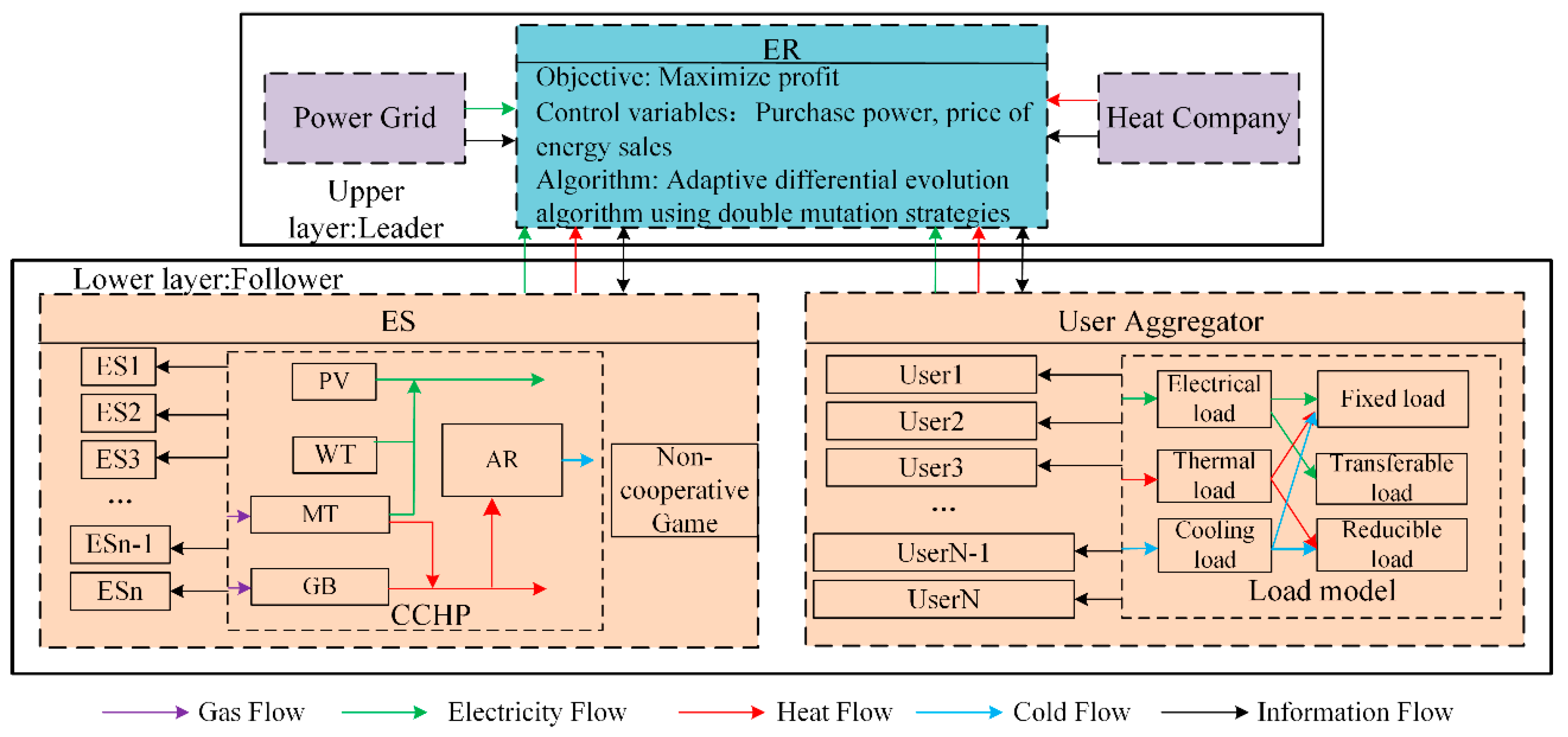
4. Two-Level Game Model

4.1. The Model of Master–Slave Game

From the aforementioned description, it can be inferred that the ES and user aggregator are optimized in accordance with the decision of the ER. Furthermore, the optimized result exerts an influence on the subsequent decision of the ER; the three decisions are thus situated in a sequential order and interact with one another, thereby forming a one-master–multiple-slave two-layer game model. This model can be expressed as follows:

$$G=\left\{\begin{array}{c}ER\cup (E{S}_1,E{S}_2,\dots E{S}_i,\dots ,E{S}_n)\cup (User\_Agg);\\ {\rho }_{ER};({\delta }_{ES1},{\delta }_{ES2},\dots {\delta }_{ESi},\dots ,{\delta }_{ESn});{\delta }_{User\_Agg};\\ F_{ER};(F_{ES1},F_{ES2},\dots F_{ESi},\dots ,F_{ESn});F_{User\_Agg};\end{array}\right\}$$

(47)

(1)

Participants: The ER, ES, and user aggregator.

(2)

Strategies: The ER’s strategy comprises two elements. The first is the aggregator of the prices of electricity and heat sold to the user, and the second is the purchasing power of electricity and heat from ESi, which is expressed as ${\rho }_{ER}=\left(c_{es},c_{hs},P_{e,i},P_{h,i}\right)$. The strategy for each ES refers to the price of energy sold, which is expressed as ${\delta }_{ESi}=\left(c_{ebi},c_{hbi}\right)$. Finally, the user aggregation strategy employs the quantity of load response at each moment in time, which is expressed as ${\delta }_{User\_Agg}=\left(\Delta P_{tl,e},\Delta P_{rl,h}\right)$.

(3)

Benefits: As previously outlined, the benefits for each agent are calculated according to Equations (19), (30), and (40).

The leader is responsible for establishing the strategic approach to be employed, which is then adopted by the followers in a manner that is optimized with respect to the leader’s strategy. In the event that both parties unilaterally alter their strategies, neither side will be able to enhance their respective benefits. Consequently, the master–slave game reaches Stackelberg equilibrium [25]. The attaining of this equilibrious solution is the focus of the study presented in this paper.

$$\begin{array}{l}{F}_{ER}\left({\rho }_{ER}^{*},{\delta }_{ESi}^{*},{\delta }_{User\_Agg}^{*}\right)\ge F_{ER}\left({\rho }_{ER},{\delta }_{ESi}^{*},{\delta }_{User\_Agg}^{*}\right)\\ F_{ESi}\left({\rho }_{ER}^{*},{\delta }_{ESi}^{*},{\delta }_{User\_Agg}^{*}\right)\ge F_{ESi}\left({\rho }_{ER}^{*},{\delta }_{ESi},{\delta }_{User\_Agg}^{*}\right)\\ F_{user}\left({\rho }_{ER}^{*},{\delta }_{ESi}^{*},{\delta }_{User\_Agg}^{*}\right)\ge F_{user}\left({\rho }_{ER}^{*},{\delta }_{ESi}^{*},{\delta }_{User\_Agg}\right)\end{array}$$

(48)

4.2. The Model of the Non-Cooperative Game

In follower optimization, ESs compete with each other to develop different pricing strategies to maximize revenue. These strategies are subject to adjustment in accordance with the ER’s purchasing strategy. Consequently, the competitive pricing relationship between ESs assumes the form of a non-cooperative game, which is expressed as

$$G_{{\rm K}}=\left\{\begin{array}{c}E{S}_1,\dots ,E{S}_i,\dots E{S}_n;\\ {\rho }_{ES1},\dots ,{\rho }_{ESi},\dots ,{\rho }_{ESn};\\ F_{ES1},\dots ,F_{ESi},\dots ;F_{ESn};\end{array}\right\}$$

(49)

(1)

Participants: n ESs.

(2)

Strategy: The strategy for each ES is the price of electricity and heating, denoted as ${\rho }_{ESi}=\left(a_{be.i},a_{bh,i}\right)$.

(3)

Benefits: The value of the ES objective function, as described earlier, is calculated using Equation (30).

A Nash equilibrium is reached in a non-cooperative game when any participant is unable to alter their existing strategy in order to obtain a greater gain.

$$F_{ESi}\left({\rho }_{ESi}^{*},{\rho }_{ES-i}^{*}\right)\ge F_{ESi}\left({\rho }_{ESi},{\rho }_{ES-i}^{*}\right)$$

(50)

4.3. Game Equilibrium Solution

4.3.1. Stackelberg Equilibrium Solution

In the event that a Stackelberg equilibrium solution occurs and is unique, the following conditions must be satisfied:

(1)

The utility functions of the game participants are non-empty, continuous functions on the set of game strategies.

(2)

In accordance with the strategy adopted by the ER, a unique optimal solution exists for each ES and user aggregator.

(3)

In accordance with the strategies adopted by each ES and user aggregator, a unique optimal solution exists for the ER.

Proof. 

As the proof is valid for any time period, the subscripts for the time periods are omitted from the formula.

(1)

In accordance with the aforementioned description, the strategies of the leader ER must satisfy the conditions set forth in Equations (24)–(29), while the strategies of each ES must satisfy the conditions outlined in Equations (34)–(39). Additionally, the strategies of the user aggregator must satisfy the criteria specified in Equations (42)–(46). This ensures that the set of strategies for each participant is non-empty and tightly convex.

(2)

Once the purchased energy powers $P_{e.i}$ and $P_{h.i}$ of ER are defined, it can be observed that the return of each ES varies linearly with the decision according to Equation (30), so a unique solution is possible for each ES, which can be expressed as

$${\rho }_{eb,i}^{\prime }=a_{be,i}+b_{fe,i}{P}_{e,i}$$

(51)

$${\rho }_{hb,i}^{\prime }=a_{bh,i}\left(t\right)+b_{fh,i}{P}_{h,i}$$

(52)

Once the energy selling prices ${\rho }_{es}$ and ${\rho }_{hs}$ of the leader ER have been established, the first-order partial derivatives for $P_{ue,k}$ and $P_{uh,k}$, respectively, are obtained using Equation (40).

$$\left\{\begin{array}{l}{\displaystyle \frac{\partial F_{User\_Agg}}{\partial P_{ue,k}}}={\alpha }_{e,k}-2{\beta }_{e,k}{P}_{ue,k}-{\rho }_{es}\\ {\displaystyle \frac{\partial F_{User\_Agg}}{\partial P_{uh,k}}}={\alpha }_{h,k}-2{\beta }_{h,k}{P}_{uh,k}-{\rho }_{hs}\end{array}\right.$$

(53)

Let the first-order partial derivative of both be 0. This yields

$$\left\{\begin{array}{l}{P}_{ue,k}^{\prime }={\displaystyle \frac{{\alpha }_{e,k}-{\rho }_{es}}{2{\beta }_{e,k}}}\\ P_{uh,k}^{\prime }={\displaystyle \frac{{\alpha }_{h,k}-{\rho }_{hs}}{2{\beta }_{h,k}}}\end{array}\right.$$

(54)

The second-order partial derivatives of Equation (40) are then obtained for $P_{ue,k}$ and $P_{uh,k}$.

$$\left\{\begin{array}{l}{\displaystyle \frac{{\partial }^2{F}_{User\_Agg}}{\partial {P_{ue,k}}^2}}=-2{\beta }_{e,k}\\ {\displaystyle \frac{{\partial }^2{F}_{User\_Agg}}{\partial {P_{uh,k}}^2}}=-2{\beta }_{h,k}\end{array}\right.$$

(55)

Given that both ${\beta }_{e,k}$ and ${\beta }_{h,k}$ are positive, the second-order partial derivatives are both less than zero, indicating that the function reaches a maximum point. Consequently, there are unique optimal solutions, $P_{ue,k}^{\prime }$ and $P_{uh,k}^{\prime }$, for the user aggregator.

(3)

We assume that the ER must purchase electricity and heat from the higher level in order to satisfy user demand. Then, the optimal solutions of the ES and user aggregator obtained from the above proof are incorporated into Equation (19), and the second-order partial derivatives of $P_{e,i}$, $P_{h,i}$, ${\rho }_{es}$, and ${\rho }_{hs}$ are calculated.

$$\left\{\begin{array}{l}{\displaystyle \frac{{\partial }^2{F}_{ER}}{\partial {P_{e,i}}^2}}=-2b_{fe,i}\\ {\displaystyle \frac{{\partial }^2{F}_{ER}}{\partial {P_{h,i}}^2}}=-2b_{fh,i}\\ {\displaystyle \frac{{\partial }^2{F}_{ER}}{\partial {{\rho }_{es}}^2}}=-{\displaystyle \frac{2}{{\beta }_{e,k}}}\\ {\displaystyle \frac{{\partial }^2{F}_{ER}}{\partial {{\rho }_{hs}}^2}}=-{\displaystyle \frac{2}{{\beta }_{h,k}}}\end{array}\right.$$

(56)

Given that the variables $b_{fe,i}$, $b_{fh,i}$, ${\beta }_{e,k}$, and ${\beta }_{h,k}$ are positive, it follows that all second-order partial derivatives are less than zero. Consequently, there is a unique optimal solution for the ER that adheres to the aforementioned constraints. □

4.3.2. Nash Equilibrium for Non-Cooperative Game

Theorem 1.

A Nash equilibrium exists for a non-cooperative game (49) when the set of strategies of all participants is non-empty tightly convex, and the utility function is continuously concave with respect to the decision variables.

Proof. 

From Equations (34) to (39), it can be seen that the set of strategies employed by ES is non-empty and tightly convex. The first-order partial derivatives of the ESi’s benefit with respect to $P_{e,i}\left(t\right)$, $P_{h,i}\left(t\right)$, $P_{MT,i}\left(t\right)$, $H_{GB,i}\left(t\right)$, $P_{PV,i}\left(t\right)$, $P_{WT,i}\left(t\right)$, $P_{GB,i}\left(t\right)$, $P_{dis,i}^x\left(t\right)$, and $P_{char,i}^x\left(t\right)$ are as follows:

$$\left\{\begin{array}{c}{\displaystyle \frac{\partial F_{ES,i}}{\partial P_{e,i}\left(t\right)}}=c_{eb,i}(t)\\ {\displaystyle \frac{\partial F_{ES,i}}{\partial P_{h,i}(t)}}=c_{hb,i}(t)\\ {\displaystyle \frac{\partial F_{ES,i}}{\partial P_{MT,i}(t)}}=-2a_{MT,i}{P}_{MT,i}(t)-b_{MT,i}-{\lambda }_{MT,i}\\ {\displaystyle \frac{\partial F_{ES,i}}{\partial H_{GB,i}(t)}}=-2a_{GB,i}{H}_{GB,i}(t)-b_{GB,i}-{\lambda }_{GB,i}\\ {\displaystyle \frac{\partial F_{ES,i}}{\partial P_{e,i}(t)}}=c_{eb,i}\left(t\right)\\ {\displaystyle \frac{\partial F_{ES,i}}{\partial P_{PV,i}\left(t\right)}}=-{\lambda }_{PV,i}\\ {\displaystyle \frac{\partial F_{ES,i}}{\partial P_{WT,i}\left(t\right)}}=-{\lambda }_{WT,i}\\ {\displaystyle \frac{\partial F_{ES,i}}{\partial P_{GB,i}\left(t\right)}}=-{\lambda }_{GB,i}\\ {\displaystyle \frac{\partial F_{ES,i}}{\partial P_{chr,i}^x\left(t\right)}}=-{\sigma }_i^x\\ {\displaystyle \frac{\partial F_{ES,i}}{\partial P_{dis,i}^x\left(t\right)}}=-{\sigma }_i^x\end{array}\right.$$

For $P_{e,i}\left(t\right)$, $P_{h,i}\left(t\right)$, $P_{PV,i}\left(t\right)$, $P_{WT,i}\left(t\right)$, $P_{GB,i}\left(t\right)$, $P_{dis,i}^x\left(t\right)$, and $P_{char,i}^x\left(t\right)$, their first-order partial derivatives are all constants, indicating they are linear in the objective function (30). Further, the second-order partial derivatives with respect to $P_{MT,i}\left(t\right)$ and $H_{GB,i}\left(t\right)$ are as follows:

$$\left\{\begin{array}{c}{\displaystyle \frac{{\partial }^2{F}_{ES,i}}{\partial {\left[P_{MT,i}\left(t\right)\right]}^2}}=-2a_{MT,i}\\ {\displaystyle \frac{{\partial }^2{F}_{ES,i}}{\partial {\left[H_{GB,i}\left(t\right)\right]}^2}}=-2a_{GB,i}\end{array}\right.$$

Because $a_{MT,i}$ and $a_{GB,i}$ are positive constants, the second-order partial derivatives are strictly less than zero. That is, the objective function (30) is strictly concave, and a unique optimal solution exists. Therefore, it can be concluded that there is a Nash equilibrium in the non-cooperative game between ESs. □

5. Model Solving

The model in this paper exhibits characteristics of high dimensionality and nonlinearity and involves a multitude of optimization variables. In order to enhance its optimization capabilities and mitigate solution complexity while maintaining a balance between processing speed and accuracy, a differential evolutionary algorithm that incorporates bi-variance and adaptive crossover is employed in collaboration with the CPLEX solver (v12.6) to address the formulated model.

The model’s solution flowchart is shown in Figure 3. The solution flow is as follows:

Step 1: Input device parameters and load information. Input the parameters of the differential evolutionary algorithm: the population size is 50, F = 0.3 and is used for the double mutation strategy, and $w$ = 0.6 and is used for the adaptive crossover strategy.

Step 2: Initial population. Under the energy price cap, randomly generate the initial energy sales price for the user aggregator, and simultaneously, under the maximum energy output power limit of the ES, randomly generate the initial energy purchase power for ES.

Step 3: The ES and user aggregator utilize CPLEX (v12.6) to ascertain the optimal energy sale price and demand response volume based on Formulas (30) and (40), respectively. Subsequently, we convey these findings to the upper layer and calculate and redeem the ER’s profit at this time.

Step 4: Calculate individual fitness values using Equation (19), determine the current central solution, and calculate the similarity of the population and the individual superiority index according to Formulas (58) and (60). Then, use Formula (57) to implement mutation operations using the double mutation strategy. Compared with ordinary mutation strategies, the double mutation strategy can strengthen the global search capability of the algorithm. The double mutation strategy is

$$v_i\left(g\right)=\left\{\begin{array}{l}{x}_{r_0}\left(g\right)+\lambda \times \left(x_{center}\left(g\right)-x_{r_0}\left(g\right)\right)+F\times \left(x_{r_1}\left(g\right)-x_{r_2}\left(g\right)\right),if\mu \left(g\right)<rand\\ x_{best}\left(g\right)+F\times \left(x_{r_1}\left(g\right)-x_{r_2}\left(g\right)\right),otherwise\end{array}\right.$$

(57)

where $r_0$, $r_1$, and $r_2$ represent random integers on $\left[1,NP\right]$ that are not equal to i and not identical to each other; $\lambda$ represents a local parameter, such as 0.1; $F$ represents a random factor, with a value set at random between 0 and 1; $x_{best}\left(g\right)$ denotes the optimal individual of the population in the gth generation; and $\mu \left(g\right)$ represents the similarity of the population and can be expressed as

$${\mu }_g={\displaystyle \frac{f_{aver}\left(g\right)-f\left(x_{best}\left(g\right)\right)}{f\left(x_{worst}\left(g\right)\right)-f\left(x_{best}\left(g\right)\right)}}$$

(58)

where $f_{aver}\left(g\right)$ denotes the average fitness value of the population in the gth generation; and $f\left(x_{best}\left(g\right)\right)$ and $f\left(x_{worst}\left(g\right)\right)$ represent the optimal and worst fitness values of the population in the gth generation, respectively.

Step 5: Implement the crossover operation, generate the offspring population to send to the ES and user aggregator, implement the selection operation, store the successful crossover probabilities, and calculate and save the updated ER profit according to Formula (19). Conventional crossover strategies are characterized by fixed crossover probabilities and do not involve the global search process inherent to algorithms. In the context of adaptive crossover strategies, the crossover probabilities of all successfully updated individuals are employed to determine the crossover probabilities of each individual in the subsequent generation. This approach is conducive to updating the population. The adaptive crossover strategy is as follows:

$$C{R}_i\left(g+1\right)=\left\{\begin{array}{l}w\times C{R}_i\left(g\right)+(1-w)\times {\displaystyle \frac{{\displaystyle \sum _{CR\in S_{CR}}CR}}{N{S}_{CR}}},if{\phi }_i\left(g\right)<rand\\ \left(1-w\right)\times C{R}_i\left(g\right)+w\times {\displaystyle \frac{{\displaystyle \sum _{CR\in S_{CR}}CR}}{N{S}_{CR}}},otherwise\end{array}\right.$$

(59)

where $C{R}_i\left(g\right)$ denotes the crossover probability of the ith individual in the gth generation population; $S_{CR}$ represents the set of probabilities for all successful crossovers; $N{S}_{CR}$ represents the number of $S_{CR}$; $w$ represents the weight coefficient, which is 0.6 in this paper; and ${\phi }_i\left(g\right)$ represents the individual superiority index, which is expressed as

$${\phi }_i\left(g\right)={\displaystyle \frac{f\left(x_i\left(g\right)\right)-f\left(x_{best}\left(g\right)\right)}{f\left(x_{best}\left(g\right)\right)-f\left(x_{worst}\left(g\right)\right)}}$$

(60)

Step 6: If the maximum number of iterations have been reached, terminate the procedure and output the best solution. Otherwise, adaptively adjust the crossover probability according to Formula (59), and return to step (3).

6. Case Study

6.1. Basic Data

A community in northern China was selected as a case study to simulate and analyze the proposed CIES two-layer game model, with consideration given to IDR and the CTM. Through rigorous statistical sampling methods and standardized data processing procedures, 800 users in the community were selected for case studies. By analyzing the energy consumption habits of community users, users in the community were divided into four groups: users who prefer electricity and heat, users who prefer electricity, users who prefer heat, and users who have no preference. Given the similarity in energy output and trading between winter and summer, in this study, we conducted a simulation based on a representative day in the winter season. The proposed algorithm has been implemented in PlatEMO (v3.0), an open-source, user-friendly, and easily extendable MATLAB platform (v2018). It was run on a PC with an i7 CPU, 8 GB of RAM, and a Windows 10 operating system.

Figure 4 illustrates the electricity and heat load curves for four representative users’ profiles, with each curve representing 200 users. RU1 represents users who prefer electricity and heat, RU2 represents users who prefer electricity, RU3 represents users who prefer heat, and RU4 represents users who have no preference.

Table 2. Parameters for each typical user.

Categories of Users	Parameter	Value
RU1 (users who prefer both electricity and heat)	${\alpha }_{e,1},{\beta }_{e,1}$	1.6, 0.004
	${\alpha }_{h,1},{\beta }_{h,1}$	1.2, 0.003
RU2 (users who prefer electricity)	${\alpha }_{e,2},{\beta }_{e,2}$	1.6, 0.004
	${\alpha }_{h,2},{\beta }_{h,2}$	1.0, 0.005
RU3 (users who prefer heat)	${\alpha }_{e,3},{\beta }_{e,3}$	1.4, 0.006
	${\alpha }_{h,3},{\beta }_{h,3}$	1.2, 0.003
RU4 (general users)	${\alpha }_{e,4},{\beta }_{e,4}$	1.5, 0.005
	${\alpha }_{h,4},{\beta }_{h,4}$	1.1, 0.004

presents the energy preference coefficients for each user profile. Two ESs were selected for simulation. The prediction curves of PV and WT power generation of the two ESs on a typical day in winter are illustrated in Figure 5. The operating parameters of each piece of equipment in each ES are illustrated in

Table 3. Parameters of each ES and CTM.

Parameter	Value	Parameter	Value
$P_{MT,1,\max }$ /kW	500	${\sigma }_1^2$	0.02
$P_{GB,1,\max }$ /kW	600	${\eta }_{MT,1}$	0.41
$r_{MT,1}^d,r_{MT,1}^u$ /kW	−230, 230	${\gamma }_{MT,1}$	0.09
$r_{GB,1}^d,r_{GB,1}^u$ /kW	−300, 300	${\eta }_{WHB,1}$	0.85
$P_{MT,2,\max }$ /kW	450	${\sigma }_2^1$	0.007
$P_{GB,2,\max }$/kW	500	${\sigma }_2^2$	0.02
$r_{MT,2}^d,r_{MT,2}^u$ /kW	−220, 220	${\eta }_{MT,2}$	0.38
$r_{GB,2}^d,r_{GB,2}^u$/kW	−250, 250	${\gamma }_{MT,2}$	0.07
${\lambda }_{1,1},{\lambda }_{2,1},{\lambda }_{3,1},{\lambda }_{4,1}$	0.016, 0.018, 0.02, 0.02	${\eta }_{WHB,2}$	0.83
${\lambda }_{1,1},{\lambda }_{2,1},{\lambda }_{3,1},{\lambda }_{4,1}$	0.02, 0.02, 0.015, 0.015	$\psi$	0.252
${\sigma }_1^1$	0.0068	$\epsilon$ /%	25

. The feed-in tariff of the grid company is CNY 0.35/(kWh). In the purchasing of electricity from the grid company, we have adopted time-of-use price, and the prices in the peak, flat, and valley periods are CNY 1.25, 0.4, and 0.8/(kWh), respectively. The price of heat purchased from the heat company is CNY 0.62/(kWh). The maximum and minimum limits of the ER’s heat sales price are CNY 0.6 and 0.1/(kWh), respectively.

6.2. Analysis of Game Equilibrium Results

The optimization iteration curves for each agent in the system under Mode 5 are presented in Figure 6. When the optimization iteration curve converges, the game reaches equilibrium, the model’s optimization results reach the optimal state, and all entities make the optimal decisions. Figure 6 shows a convergence trend around the 70th iteration, while the convergence trend of each agent in the system was distinct. Prior to the 20th iteration, there was a notable increase in ER revenue as the number of iterations increased. The revenues of ES1 and ES2 fluctuated irregularly, a consequence of the competitive pricing interaction between the two agents. The revenue of the user aggregator demonstrated volatility and a downward trend, which is attributable to the ER incrementally increasing the energy sales prices with a view to maximizing profits. Specifically, In the iterative process of the game, ER will gradually increase the energy sales price to improve its profits. This will cause the energy purchase costs of user aggregators to rise, thereby reducing their profits. Volatility is caused by changes in energy prices during the iterative process, which cause users to change their demand response volume and energy consumption. Following the 20th iteration, the ER’s revenue exhibited a gradual increase, while the user aggregator’s revenue demonstrated a corresponding decrease. Additionally, the revenues of ES1 and ES2 reached a state of equilibrium. Until approximately the 70th iteration, the revenues of each agent remained constant, and the game reached equilibrium. At this moment, the revenues of the ER, the user aggregator, ES1, and ES2 were stable at CNY 7810, 10794, 2283, and 2295, respectively.

The energy sales price strategy of energy suppliers for when the game reaches equilibrium is shown in Figure 7. The analysis demonstrates that the electricity and heat selling prices of ES1 and ES2 manifested a distinct pattern of high and low values with notable regularity. This was due to the fact that there was a non-cooperative game being played between ESs, with both parties expecting to purchase more energy from the ER. Consequently, they were compelled to engage in competitive pricing strategies to secure lower energy prices. As evidenced by Equations (36) and (37), there was a discernible linear correlation between the energy selling price set by the ES and the energy purchases made by the ER. In other words, as the energy purchases of the ER increased, so did the energy selling price set by the ES.

6.3. Optimal Scheduling Analysis

Figure 8 and Figure 9 illustrate the optimal energy pricing strategy for the ER following the establishment of game equilibrium and the electric heat load profile after IDR, respectively. In Figure 9a, the blue columns represent the electrical load transfer, with the top and bottom of the horizontal axis representing inward and outward electrical load transfer, respectively. Comparing Figure 8 and Figure 9a, we see that, between 0:00 and 9:00 and 14:00 and 17:00, users’ electricity loads shift, corresponding to the lower ER electricity prices during these periods. To reduce their electricity costs, users will shift some of their transferable electricity demand to these time slots. Conversely, between 10:00 and 12:00 and 18:00 and 23:00, users shift their electricity load outwards, as the ER electricity prices are higher during these periods. Users will reduce their electricity demand during these time slots. Therefore, influenced by electricity prices, some of the adjustable electricity load demand of users will shift, increasing electricity demand during off-peak periods and reducing electricity demand during peak periods. These changes in user electricity load reflect the “peak-shaving and valley-filling” effect of demand response. Comparing Figure 8 and Figure 9b, we see that the price of selling heat set by the ER remains relatively consistent across most time periods, and the reduction in heat load following user demand response also remains relatively consistent during these periods. However, between 14:00 and 16:00, the ER’s heat sales price is relatively low, resulting in a smaller reduction in user heat load. Therefore, the reduction in user heat load is correlated with the ER’s heat sales price; when the heat price is high, the reduction in heat load is higher, and when the heat price is low, the reduction in user heat load is lower, with users tending to consume more heat energy.

Figure 8 and Figure 9 show that IDR is effective and important for scheduling CIES operations. Designing reasonable time-of-use electricity pricing strategies can successfully stimulate load shifting behavior among electricity users, achieve significant peak shaving and valley filling effects, and optimize CIES operations. Moreover, IDR for heat is primarily achieved by adjusting energy consumption intensity based on real-time or time-of-use heat prices. The degree of IDR is directly and positively correlated with the level of heat prices.

The equilibrium in the system’s electricity and heat supply and demand is illustrated in Figure 10. An analysis of Figure 10a reveals that, with regard to the scheduling of electric energy, both ES1 and ES2 assigned priority to the supply of wind and PV power based on considerations related to economics and reduced carbon emissions. In the event of insufficient renewable energy output, it was supplemented with gas turbine power generation. Concurrently, comparing Figure 7 and Figure 10a demonstrates that the electric storage equipment of ES1 and ES2 was charged when the electricity price was low and the output of renewable energy was high and discharged when the electricity price was high and there was a shortage of renewable energy. Figure 10b shows that for heat scheduling, ES1 and ES2 gave priority to the WHB for heat supply based on economic factors, and when the waste heat recovered from the WHB was insufficient, it was supplemented with heat produced by the GB. Figure 7 and Figure 10b together illustrate that the heat storage apparatus of both ES1 and ES2 chose to accumulate heat when the heat price was low and released it when the price was high.

The above results indicate that, through optimization of the proposed algorithm, CIES achieves multi-energy complementarity and synergy. The system organically integrates elements such as electricity, heat, renewable energy, energy storage, and IDR. Waste heat generated during electricity production is effectively recovered for heating purposes, enabling hierarchical energy utilization. Through their respective supply-side, energy storage-side, and demand-side strategies, as well as the coordination of price signals, the electricity and heat subsystems achieve overall economic, low-carbon, efficient, and reliable operation.

6.4. Analysis of Different Operational Modes

In an attempt to gain further insight into the economic and carbon-reduction effects of the proposed model, five distinct operational modes were devised for analysis. The operation modes are outlined in

Table 4. The operation modes.

Operation Mode	User Classification	IDR	CTM	Non-Cooperative Game
Mode 1	×	√	√	√
Mode 2	√	×	√	√
Mode 3	√	√	×	√
Mode 4	√	√	√	×
Mode 5 (this study)	√	√	√	√

, where a “√” indicates that the strategy is implemented and an “×” indicates that the strategy is not implemented. Mode 5 is the mode recommended in this paper, which considers user classification, IDR, the CTM, and the non-cooperative game among ESs. In Mode 1, the preference parameters displayed by the users take the average values of the preference parameters of the four types of typical users employed in Mode 5. In Mode 4, energy is sold at a fixed price, which is the average of the price set by the bidding process amongst energy suppliers under Mode 5.

Table 5. Optimization results for different modes.

Operational Indicator		Mode 1	Mode 2	Mode 3	Mode 4	Mode 5
Revenue (CNY)	ER	7728	8370	7871	8233	7810
	user aggregator	7737	8581	10,911	10,901	10,794
	ES1	1669	1440	3356	1786	2283
	ES2	3114	1590	4033	1934	2295
Carbon emissions (kg)	ER	2406	2997	7831	3150	2611
	ES1	12,249	13,622	12,128	10,611	10,446
	ES2	11,890	16,528	17,862	12,608	12,659
Total carbon emissions (kg)		26,545	33,147	37,821	26,369	25,716
Carbon trading costs (CNY)	ES1	1443	1733	-	1156	1299
	ES2	1388	2258	-	1501	1890

reveals the revenue generated by each agent under the five modes, as well as the carbon emissions and carbon costs associated with the ER and each ES. A comparative analysis of the five modes indicates that the consideration of both IDR and the CTM can effectively reduce carbon emissions, aligning with the objective of a low-carbon system. Furthermore, the implementation of user classification and a non-cooperative game among ESs can enhance the revenue of the user aggregator and each ES. The results substantiate the efficacy of the proposed model in enhancing the revenues for each agent and reducing carbon emissions.

A comparison of Mode 1 with Mode 5 reveals a 39.51% increase in user aggregator revenue when user classification is considered. Simultaneously, the revenue generated per kWh increased by 39.10%. This is due to the fact that, following user classification and as influenced by the energy price set by the ER, different users are able to determine the optimal load response based on their own energy preference factors. Consequently, the user aggregator is able to participate in IDR more effectively. It can therefore be concluded that the consideration of user classification significantly improves the revenue generated on the user side. Furthermore, following the introduction of user categorization, the benefits of ES1 decrease, while those of ES2 increase, indicating that user categorization influences the ER’s decision-making processes. As a result, the ER’s purchasing of energy from each ES undergoes a corresponding alteration, leading to a change in the benefits for the ES.

A comparison of Mode 2 with Mode 5 reveals that, after considering IDR, there was an increase of 25.79% in user aggregator revenue and a 17.79% decrease in the total carbon emissions of the system. Simultaneously, the revenue generated per kWh increased by 33.02%, while the carbon emissions generated per kWh decreased by 15.04%. This is attributable to the fact that, following the consideration of IDR on the user side, users are able to respond in a manner that is beneficial to their own interests, guided by the price. The user’s heat load is reduced at the peak of the heat price, the electricity load is leveled off at the peak of the electricity price, the load demand of the system is lowered, and accordingly, the user energy costs are reduced. Furthermore, the reduction in the heat load on the user side results in a decrease in the heat load purchased by the ER from the ES, a reduction in the output of the ES’s equipment, and a subsequent reduction in carbon emissions.

A comparison of Mode 3 with Mode 5 reveals that the total carbon emissions of the system were reduced by 32.01% following the introduction of the CTM. Simultaneously, the carbon emissions generated per kWh decreased by 27.89%. However, this reduction in carbon emission was accompanied by a decrease in revenue for ES1 and ES2, with reductions of 31.97% and 43.09%, respectively. The introduction of carbon trading costs caused ES1 and ES2 to adopt more economical power generation strategies, which increased the costs of ES1 and ES2 but reduced their carbon emissions. At the same time, the introduction of carbon trading costs also increased the costs to the ER, prompting the ER to reduce its electricity and heat purchases from the power grid and heating companies, thereby reducing carbon emissions. In addition, the carbon emissions of the ER in Mode 3 increased by 200% compared to Mode 5, suggesting that the lack of a cost constraint on carbon emissions leads the ER to buy more electricity and heat from the upper level.

A comparison of Model 4 with Model 5 reveals that ES1 and ES2 exhibited improvements of 27.83% and 18.67%, respectively, when the non-cooperative game between ESs was taken into account. Simultaneously, the revenue generated per kWh by ES1 and ES2 increased by 23.56% and 13.16%, respectively. This is due to the fact that when ESs engage in a non-cooperative game with one another, they compete via price to achieve greater ER energy purchases in comparison to a fixed-price strategy. This allows them to better engage in the energy market and improve their own financial returns.

7. Conclusions

This paper addresses optimal operation in the context of the interests of multiple agents in a CIES. It introduces an ER as the manager of the CIES and multiple ESs and user aggregators as followers. Furthermore, it proposes a two-level game optimization operation strategy that considers IDR and the CTM. The findings of the simulation analysis can be summarized as follows:

(1)

The introduction of non-cooperative games between ESs has been demonstrated to be an effective strategy for increasing profits. The implementation of non-cooperative game strategies among ESs can enhance the profitability of ES1 and ES2 by 27.83% and 18.67%, respectively. In comparison to a fixed energy sales price strategy, a non-cooperative game allows ESs to participate more effectively in market competition, which is conducive to the synergistic and optimal development of multiple agents.

(2)

The introduction of IDR can increase user revenue while reducing the system’s carbon emissions. The incorporation of IDR into the optimization model has been demonstrated to enhance user-side benefits by 25.79% while simultaneously curtailing the system’s carbon emissions by 22.42%. Concurrently, the introduction of the CTM can significantly reduce the carbon emissions of the system. The incorporation of the CTM results reduces the benefits associated with ES1 and ES2 by 31.97% and 43.09%, respectively. However, this is accompanied by a 32.01% decrease in the system’s carbon emissions, which aligns with the present requirements for achieving low-carbon IES.

(3)

Classifying users enables those on the demand side to participate more effectively in the demand–response market, thereby increasing revenue. The implementation of user classification can enhance user-level benefits by up to 39.51%. Once users have been categorized according to their energy-use characteristics, they are better positioned to engage with IDR and derive the greatest benefit from it.

This paper does not address the effects of uncertainty regarding the WT and PV on optimization. In future research, the uncertainty of renewable energy outputs will be considered, along with an in-depth study of the issue of incomplete information in the game amongst IES agents.

References

1. Firouzi, M.; Samimi, A.; Salami, A. Reliability evaluation of a composite power system in the presence of renewable generations. Reliab. Eng. Syst. Saf. 2022, 222, 108396. [Google Scholar] [CrossRef]
2. Zhang, G.M.; Wang, W.; Chen, Z.Y.; Li, R.L.; Niu, Y.G. Modeling and optimal dispatch of a carbon-cycle integrated energy system for low-carbon and economic operation. Energy 2022, 240, 122795. [Google Scholar] [CrossRef]
3. Fan, W.; Liu, Q.; Wang, M.Y. Bi-Level Multi-Objective Optimization Scheduling for Regional Integrated Energy Systems Based on Quantum Evolutionary Algorithm. Energies 2021, 14, 4740. [Google Scholar] [CrossRef]
4. Wang, Y.L.; Wang, Y.D.; Huang, Y.J.; Yu, H.Y.; Du, R.T.; Zhang, F.L.; Zhang, F.; Zhu, J. Optimal Scheduling of the Regional Integrated Energy System Considering Economy and Environment. IEEE Trans. Sustain. Energy 2019, 10, 1939–1949. [Google Scholar] [CrossRef]
5. Ma, Y.; Wang, H.; Hong, F.; Yang, J.; Chen, Z.; Cui, H.; Feng, J. Modeling and optimization of combined heat and power with power-to-gas and carbon capture system in integrated energy system. Energy 2021, 236, 121392. [Google Scholar] [CrossRef]
6. Qiu, S.; Chen, J.; Mao, C.; Duan, Q.; Ma, C.; Liu, Z.; Wang, D. Day-ahead optimal scheduling of power–gas–heating integrated energy system considering energy routing. Energy Rep. 2022, 8, 1113–1122. [Google Scholar] [CrossRef]
7. Parrish, B.; Heptonstall, P.; Gross, R.; Sovacool, B.K. A systematic review of motivations, enablers and barriers for consumer engagement with residential demand response. Energy Policy 2020, 138, 111221. [Google Scholar] [CrossRef]
8. Wang, Y.Y.; Guo, T.T.; Cheng, T.C.E.; Wang, N. Evolution of blue carbon trading of China’s marine ranching under the blue carbon special subsidy mechanism. Ocean Coast. Manag. 2022, 222, 106123. [Google Scholar] [CrossRef]
9. Li, P.; Wang, Z.X.; Wang, N.; Yang, W.H.; Li, M.Z.; Zhou, X.C.; Yin, Y.; Wang, J.; Guo, T. Stochastic robust optimal operation of community integrated energy system based on integrated demand response. Int. J. Electr. Power Energy Syst. 2021, 128, 106735. [Google Scholar] [CrossRef]
10. Zheng, S.L.; Sun, Y.; Li, B.; Qi, B.; Zhang, X.D.; Li, F. Incentive-based integrated demand response for multiple energy carriers under complex uncertainties and double coupling effects. Appl. Energy 2021, 283, 116254. [Google Scholar] [CrossRef]
11. Wang, Y.L.; Li, Y.W.; Zhang, Y.F.; Xu, M.M.; Li, D.X. Optimized operation of integrated energy systems accounting for synergistic electricity and heat demand response under heat load flexibility. Appl. Therm. Eng. 2024, 243, 122640. [Google Scholar] [CrossRef]
12. Liang, Z.; Liang, C.; Zhu, W.W.; Ling, L.Y.; Cai, G.W.; Hai, K.L. Research on the optimal allocation method of source and storage capacity of integrated energy system considering integrated demand response. Energy Rep. 2022, 8, 10434–10448. [Google Scholar]
13. Wang, J.; Xing, H.J.; Wang, H.X.; Xie, B.J.; Luo, Y.F. Optimal Operation of Regional Integrated Energy System Considering Integrated Demand Response and Exergy Efficiency. J. Electr. Eng. Technol. 2022, 17, 2591–2603. [Google Scholar] [CrossRef]
14. Zhou, W.; Sun, Y.H.; Zong, X.J.; Zhou, H.W.; Zou, S. Low-carbon economic dispatch of integrated energy system considering carbon trading mechanism and LAES-ORC-CHP system. Front. Energy Res. 2023, 11. [Google Scholar] [CrossRef]
15. Liu, X.O. Research on optimal placement of low-carbon equipment capacity in integrated energy system considering carbon emission and carbon trading. Int. J. Energy Res. 2022, 46, 20535–20555. [Google Scholar] [CrossRef]
16. Cheng, X.; Zheng, Y.; Lin, Y.; Chen, L.; Wang, Y.Q.; Qiu, J. Hierarchical operation planning based on carbon-constrained locational marginal price for integrated energy system. Int. J. Electr. Power Energy Syst. 2021, 128, 106714. [Google Scholar] [CrossRef]
17. Pan, D.; Zhang, L.; Wang, B.; Jia, J.X.; Song, Z.M.; Zhang, X. Multi-objective planning of integrated energy system based on CVaR under carbon trading mechanism. Front. Energy Res. 2024, 12. [Google Scholar] [CrossRef]
18. Li, L.L.; Miao, Y.; Lin, C.J.; Qu, L.N.; Liu, G.C.; Yuan, J.P. Low-carbon Economic Operation Optimization of Integrated Energy System Considering Carbon Emission Sensing Measurement System and Demand Response: An Improved Northern Goshawk Optimization Algorithm. Sens. Mater. 2023, 35, 4417–4437. [Google Scholar] [CrossRef]
19. Sun, H.B.; Sun, X.M.; Kou, L.; Ke, W.D. Low-Carbon Economic Operation Optimization of Park-Level Integrated Energy Systems with Flexible Loads and P2G under the Carbon Trading Mechanism. Sustainability 2023, 15, 15203. [Google Scholar] [CrossRef]
20. Chen, M.; Lu, H.; Chang, X.; Liao, H. An optimization on an integrated energy system of combined heat and power, carbon capture system and power to gas by considering flexible load. Energy 2023, 273, 127203. [Google Scholar] [CrossRef]
21. Zeng, X.Q.; Wang, J.; Zhou, Y.; Li, H.J. Optimal configuration and operation of the regional integrated energy system considering carbon emission and integrated demand response. Front. Energy Res. 2023, 11. [Google Scholar] [CrossRef]
22. Huang, Y.J.; Wang, Y.D.; Liu, N. A two-stage energy management for heat-electricity integrated energy system considering dynamic pricing of Stackelberg game and operation strategy optimization. Energy 2022, 244, 122576. [Google Scholar] [CrossRef]
23. Yarar, N.; Yoldas, Y.; Bahceci, S.; Onen, A.; Jung, J. A Comprehensive Review Based on the Game Theory with Energy Management and Trading. Energies 2024, 17, 3749. [Google Scholar] [CrossRef]
24. Zhang, Y.Y.; Zhao, H.R.; Li, B.K.; Wang, X.J. Research on dynamic pricing and operation optimization strategy of integrated energy system based on Stackelberg game. Int. J. Electr. Power Energy Syst. 2022, 143, 108446. [Google Scholar] [CrossRef]
25. Wang, R.; Cheng, S.; Zuo, X.W.; Liu, Y. Optimal management of multi stakeholder integrated energy system considering dual incentive demand response and carbon trading mechanism. Int. J. Energy Res. 2022, 46, 6246–6263. [Google Scholar] [CrossRef]
26. Wang, Y.L.; Liu, Z.; Wang, J.Y.; Du, B.X.; Qin, Y.M.; Liu, X.L.; Lin, L. A Stackelberg game-based approach to transaction optimization for distributed integrated energy system. Energy 2023, 283, 128475. [Google Scholar] [CrossRef]
27. Wang, Y.D.; Hu, J.J.; Liu, N. Energy Management in Integrated Energy System Using Energy–Carbon Integrated Pricing Method. IEEE Trans. Sustain. Energy 2023, 14, 1992–2005. [Google Scholar] [CrossRef]
28. Yuan, X.L.; Guo, Y.; Cui, C.; Cao, H. Time-of-Use Pricing Strategy of Integrated Energy System Based on Game Theory. Processes 2022, 10, 2033. [Google Scholar] [CrossRef]
29. Li, P.; Wang, Z.X.; Yang, W.H.; Liu, H.T.; Yin, Y.X.; Wang, J.H.; Guo, T. Hierarchically partitioned coordinated operation of distributed integrated energy system based on a master-slave game. Energy 2021, 214, 119006. [Google Scholar] [CrossRef]
30. Li, S.R.; Zhang, L.H.; Nie, L.; Wang, J.N. Trading strategy and benefit optimization of load aggregators in integrated energy systems considering integrated demand response: A hierarchical Stackelberg game. Energy 2022, 249, 123678. [Google Scholar] [CrossRef]
31. Latifi, M.; Rastegarnia, A.; Khalili, A.; Vahidpour, V.; Sanei, S. A distributed game-theoretic demand response with multi-class appliance control in smart grid. Electr. Power Syst. Res. 2019, 176, 105946. [Google Scholar] [CrossRef]
32. Shen, J.R. Low-carbon optimal dispatch of campus integrated energy system considering flexible interactions between supply and demand. Int. J. Electr. Power Energy Syst. 2024, 156, 109776. [Google Scholar] [CrossRef]
33. Yan, H.R.; Hou, H.J.; Deng, M.; Si, L.G.; Wang, X.; Hu, E.; Zhou, R. Stackelberg game theory based model to guide users’ energy use behavior, with the consideration of flexible resources and consumer psychology, for an integrated energy system. Energy 2024, 288, 129806. [Google Scholar] [CrossRef]
34. Lu, Q.; Guo, Q.S.; Zeng, W. Optimal dispatch of community integrated energy system based on Stackelberg game and integrated demand response under carbon trading mechanism. Appl. Therm. Eng. 2023, 219, 119508. [Google Scholar] [CrossRef]
35. Hou, H.; Ge, X.D.; Yan, Y.L.; Lu, Y.C.; Zhang, J.; Dong, Z.Y. An integrated energy system “green-carbon” offset mechanism and optimization method with Stackelberg game. Energy 2024, 294, 130617. [Google Scholar] [CrossRef]
36. Zhang, Y.J.; Peng, Y.L.; Ma, C.Q.; Shen, B. Can environmental innovation facilitate carbon emissions reduction? Evidence from China. Energy Policy 2017, 100, 18–28. [Google Scholar] [CrossRef]
37. Yu, S.M.; Fan, Y.; Zhu, L.; Eichhammer, W. Modeling the emission trading scheme from an agent-based perspective: System dynamics emerging from firms’ coordination among abatement options. Eur. J. Oper. Res. 2020, 286, 1113–1128. [Google Scholar] [CrossRef]
38. Li, Y.; Wang, C.L.; Li, G.Q.; Chen, C. Optimal scheduling of integrated demand response-enabled integrated energy systems with uncertain renewable generations: A Stackelberg game approach. Energy Convers. Manag. 2021, 235, 113996. [Google Scholar] [CrossRef]
Figure 1. Architecture of CIES.
Processes 13 02091 g001
Figure 2. CCHP system diagram.
Processes 13 02091 g002
Figure 3. Model solving flow.
Processes 13 02091 g003
Figure 4. Typical users’ load curves; (a) typical users electricity load curves; (b) typical users heat load curves.
Processes 13 02091 g004
Figure 5. Wind and PV curves for each ES.
Processes 13 02091 g005
Figure 6. Energy sales prices of ES1 and ES2.
Processes 13 02091 g006
Figure 7. Optimization iteration curves for each agent.
Processes 13 02091 g007
Figure 8. Energy sales prices set by the ER. (a) electricity sales price of ER; (b) heat sales price of ER.
Processes 13 02091 g008
Figure 9. Electricity and heat load curves before and after DR. (a) electricity load curves before and after demand response; (b) heat load curves before and after demand response.
Processes 13 02091 g009
Figure 10. Electricity and thermal power supply and demand balance diagrams. (a) electricity power supply and demand balance diagrams; (b) thermal power supply and demand balance diagrams.
Processes 13 02091 g010