Abstract
The results of core flooding experiments can guide the formulation of development plans for similar oil reservoirs. However, for cores from heavy oil reservoirs, asphaltene deposition often occurs during flooding due to changes in pressure, temperature, and petroleum composition, affecting the determination of injection parameters. Taking core samples from the Xia 018 well block as the research object, this study determined that the crude oil sample exhibits normal CO2 sensitivity based on PVT experiments and core flooding results. A corresponding asphaltene precipitation model was established and coupled with core-scale numerical simulation, forming an integrated core-scale numerical simulation method considering asphaltene precipitation. Through orthogonal experimental design, the optimized fracturing production parameters for Well Y were determined as follows: fracturing stage length of 1000 m, CO2 injection volume of 100 m3 per stage, fluid volume per stage of 1000 m3, proppant volume of 1000 m3, and injection rate of 14 m3/min. Finally, the optimized parameters were applied to simulate a case well, where the asphaltene deposition model combined with pressure nephograms during production provided effective guidance on unplugging timing. Compared with results without using the asphaltene deposition model, cumulative production decreased by 1300 m3 when the model was applied. These findings can provide a reference for the development of similar reservoirs.
1. Introduction
China possesses abundant unconventional oil and gas reserves, among which heavy oil reservoirs, as a crucial type of unconventional reservoirs, will become important alternative energy sources in the future [1,2,3,4]. CO2 has long been widely applied in enhanced oil recovery (EOR) research. On one hand, CO2 demonstrates favorable miscibility with in-situ crude oil. Its dissolution effectively reduces oil interfacial tension and viscosity, thereby improving crude oil mobility in reservoirs, making it extensively utilized in heavy oil reservoir development [5,6,7,8,9]. On the other hand, the application of CO2 resources in oilfield development aligns with the Carbon Capture, Utilization, and Storage (CCUS) policy, serving as a vital measure to mitigate the global climate crisis.
During CO2 injection for enhanced heavy oil recovery, asphaltene precipitation tends to occur [10,11,12,13,14,15]. Numerous domestic and international scholars have investigated the mechanisms of asphaltene generation through CO2-heavy oil interactions, establishing various asphaltene deposition models [16,17,18,19,20,21,22,23]. Mehdi Mahdavifar and colleagues employed real-time microfluidic experiments and a lattice Boltzmann immersed boundary numerical model to investigate pore-scale asphaltene deposition. The experimental results directly observed porosity reduction in different pore geometries, providing a detailed explanation of asphaltene deposition phenomena [24,25,26]. Hassan Sadeghi Yamchi and others conducted numerical simulations of asphaltene deposition induced by solvent injection by implementing liquid-liquid equilibrium (LLE) data and a reaction-based non-equilibrium mass transfer model, exploring the interaction between viscous fingering and asphaltene deposition during dimethyl ether (DME) injection. This study was applied in solvent-based recovery processes and paved the way for integrating LLE data into numerical simulations of asphaltene deposition [27,28]. Nasser Sabet and co-authors studied the mixing kinetics of paraffin solvents with oil during miscible displacement for enhanced oil recovery in porous media, proposing a rigorous formulation of the problem physics and performing high-resolution nonlinear numerical simulations to investigate the impacts of asphaltene precipitation/deposition and the resulting formation damage [29,30]. Moreover, heavy oil extraction requires collaborative optimization of drilling techniques and reservoir modification. For instance, horizontal well segmental fracturing can expand the oil drainage area [31], while acid fracturing before CO2 injection improves reservoir permeability [32]. As Li et al. demonstrated in hydrate reservoir studies of the northern South China Sea, the coupling effect of wellbore stability and fluid production significantly influences development efficiency [31]. Similarly, CO2 flooding in heavy oil reservoirs requires considering the impact of fracturing stage length on fluid distribution, aligning with Li et al.’s concept of ‘wellbore-reservoir collaborative modification’ [32].
However, the traditional integrated numerical simulation workflow cannot directly account for the impact of asphaltene changes on production, and since asphaltene plays a pivotal role in production processes, this study takes this as a starting point. Using the Xia 018 well block as an example, core flooding experiments and core-scale numerical simulations were conducted. By coupling the heavy oil component model and the asphaltene deposition model developed based on PVT experimental results for the block, an integrated core-scale numerical simulation method considering asphaltene precipitation was formed. Furthermore, the calibrated asphaltene deposition model was applied to optimize the parameters for CO2 fracturing injection production in Well Y of the block, providing reasonable production recommendations.
2. Interaction Mechanism Between CO2 and Heavy Oil
The dissolution of CO2 in crude oil and its subsequent alteration of oil properties constitute critical factors in enhancing oil recovery through CO2 flooding. Upon injection into crude oil, CO2 reduces interfacial tension between oil molecules, induces volumetric expansion, and decreases oil viscosity, thereby significantly improving fluid mobility. However, this process also disrupts the equilibrium between resin molecules and asphaltenes in crude oil, leading to asphaltene deposition. For different types of heavy oil, the interaction patterns between CO2 and heavy oil vary considerably, thus necessitating experimental investigations to elucidate these mechanisms and provide data support for subsequent numerical simulations.
2.1. Oil Swelling Tests
The oil sample was selected from the Xia 018 well block, located in the eastern part of the Junggar Basin. The reservoir structure generally presents a nose-shaped structure with a north-high and south-low trend, and the formation dip angle is 1.7–9.1°. The oil-bearing series is the Jurassic BD Formation, with a maximum thickness of 190 m. The lithology is mainly gray-green medium sandstone and fine sandstone, which is divided into sublayers a, b, and c from bottom to top. The viscosity of the degassed oil on the ground at 50 °C is 85–18,334 mPa·s, which is greatly affected by faults, making it a typical heavy oil reservoir.
Following SY/T 5542-2009 “Test Method for Reservoir Fluid Physical Properties” [33] and referencing the phase behavior test report of formation fluids from Reservoir Xia 018, formation crude oil was reconstituted under conditions of 51.8 °C and the current average reservoir pressure of 31.75 MPa. The reconstitution results of the obtained samples are presented in Table 1.

Table 1.
Reconstituted crude oil property.
To investigate phase compatibility characteristics of different gas injection schemes and elucidate the mechanisms of enhanced oil recovery (EOR) through gas injection, swelling experiments were conducted on formation crude oil under gas injection. These experiments measured key high-pressure physical properties including saturation pressure, formation volume factor, swelling factor, gas-oil ratio, density, and viscosity after gas injection.
The gas injection swelling tests were performed using a DBR visual PVT system (DBR Systems Inc., Calgary, AB, Canada), and the schematic diagram is illustrated in Figure 1 and Figure 2.
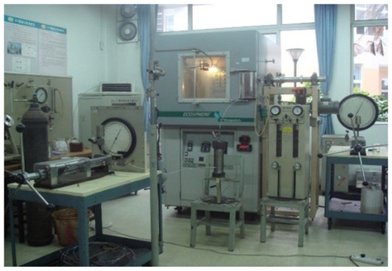
Figure 1.
DBR visual PVT system (DBR, Canada).
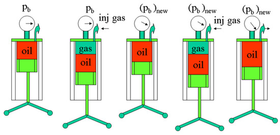
Figure 2.
Schematic Diagram of Gas Injection Swelling Experiment.
Experimental Workflow:
- Referencing the phase behavior test report of formation fluids from Well B, formation crude oil was reconstituted under conditions of 51.8 °C and reservoir pressure of 31.75 MPa;
- Prior to testing, the PVT instrument was thoroughly cleansed, purged with high-pressure nitrogen, oven-dried at experimental temperatures, and evacuated;
- The equilibrated crude oil was transferred into the PVT instrument, stabilized to the current reservoir temperature and pressure conditions, and its volume was measured;
- Injection gases (CO2 and dry gas) were injected incrementally from low to high percentages into the PVT cell. The mixture was pressurized and agitated until single-phase stability was achieved. Phase behavior characteristics (saturation pressure, Pb) and high-pressure physical properties (formation volume factor, density, viscosity, swelling factor, gas-oil ratio) under varying gas injection percentages were measured. Gas injection volume versus high-pressure property curves were subsequently plotted.
During testing, gas injection volumes were incrementally increased in 10% steps (typically 5–6 data points). Results were analyzed alongside phase behavior simulations to clarify post-injection phase evolution.
Dry gas injection (97.12% methane + 2.88% ethane) revealed that the formation crude oil exhibited heavy components with high density and viscosity. Moderate solubilization and swelling effects were observed post-injection. Rapid saturation pressure increase occurred during gas injection. Limited improvement in crude oil physical properties and moderate gas-oil compatibility were noted. The experimental results of CO2 injection into in-situ crude oil demonstrate that after CO2 is introduced, the crude oil exhibits significant solubilization and swelling, with a moderate rate of increase in saturation pressure—conditions favorable for solution gas drive. The injected gas improves crude oil’s physical properties to a certain extent, and gas injection shows good compatibility. Detailed experimental results are summarized in Table 2.
Table 2.
Test Results of Gas Injection Swelling Experiments (dry gas/CO2).
CO2 injection into formation crude oil demonstrates significant viscosity reduction effects. However, due to the relatively high subsurface density of CO2, the density alteration of crude oil post-CO2 injection remains marginal.
Comparative analysis of swelling test results between dry gas and CO2 injection reveals:
- Enhanced Phase Compatibility: CO2 exhibits superior phase compatibility with formation crude oil compared to dry gas;
- Lower Saturation Pressure: Equivalent gas injection volumes yield reduced saturation pressure under CO2 flooding conditions;
- EOR Mechanism Superiority: This pressure reduction facilitates solubility-driven swelling effects, substantially improving oil recovery efficiency.
2.2. Asphaltene Precipitation Experiments
To elucidate CO2 injection characteristics and EOR mechanisms, asphaltene precipitation experiments were conducted on formation crude oil under CO2 injection, measuring the onset pressure and precipitated asphaltene content during pressure depletion. This study focused on defining asphaltene precipitation thresholds and quantifying precipitation volumes for crude oil from the Xia 018 Well Block.
Materials and apparatus used in the experiment are as follows: For materials, a 500 mL heavy oil sample, along with high-purity gases including CO2 (with a purity of ≥99.99%) and CH4 (with a purity of ≥99.95%), were employed. As for the apparatus (shown in Figure 3), a crude oil mixer with an operating range of 0–70 MPa and 0–200 °C, a Thermogravimetric Analyzer with a temperature range of 0–1200 °C, a High-Pressure Reactor capable of operating within the range of 0–70 MPa and 0–200 °C, and a RUSKA PVT System equipped with visual FC/FPC cells (operating range: 0–70 MPa, 0–200 °C) were utilized.
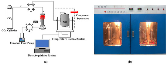
Figure 3.
Experiment setup and flow diagram for asphaltene precipitation experiments: (a) Asphaltene deposition experimental flowchart; (b) Experimental Apparatus for Asphaltene Precipitation.
The experimental steps are as follows:
- Prepare formation crude oil at 51.8 °C under saturation pressure conditions, referencing the formation fluid phase behavior test report of Well Y;
- Inject CO2 into the live oil until the current formation pressure is reached. Fully stir the mixture and allow it to stand for 12 h to ensure equilibrium;
- After standing, displace approximately 30 mL of the oil sample under constant pressure for a four-component analysis to characterize the initial fluid composition;
- Reduce the pressure in steps according to a preset pressure gradient of 3.2 MPa: decrease the pressure to 28.8 MPa in the first step, wait for flash vaporization to complete, and let the sample stand for another 12 h;
- Repeat Step 4 iteratively, reducing the pressure by 3.2 MPa each time, until the pressure drops to atmospheric pressure;
- Conduct a final four-component analysis of the sample to measure its asphaltene content. Test results are presented in Figure 4a,b.
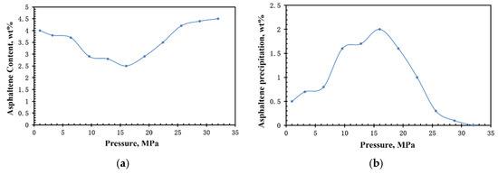 Figure 4. Asphaltene Experimental Procedures and Results: (a) Relationship Curve Between Asphaltene Content and Pressure; (b) Relationship Between Asphaltene Precipitation Amount and Pressure.
It can be seen from the figures that during the pressure reduction process with production proceeding, the asphaltene content in the extracted heavy oil samples first decreases and then increases. When asphaltene content decreases, it is because, after CO2 injection, CO2 molecules more easily diffuse into crude oil, disrupting the stable dispersed distribution of asphaltenes in crude oil. Similarly, as pressure increases, more CO2 dissolves in crude oil-high-pressure physical property experiments show that crude oil density decreases with CO2 dissolution. As a large number of CO2 molecules disperse in crude oil, due to polarity effects and molecular motion, CO2 molecules gradually occupy the surfaces of asphaltene particles, replacing resins originally covering asphaltene surfaces. Exposed asphaltene molecules then attract and agglomerate with each other, forming large particle precipitates that settle at the bottom of the PVT cell, reducing asphaltene content in the sample. As pressure further increases, the asphaltene deposition tendency strengthens. After exceeding a certain pressure (approximately 16 MPa), the asphaltene deposition amount starts to decrease with weakened tendency, possibly because when the CO2/crude oil system reaches miscibility, a further pressure increase leads to increased density of the miscible system, enhancing asphaltene dissolution capacity and reducing precipitated asphaltenes. Experiments show that the initiation pressure for asphaltene precipitation in the target block crude oil is approximately 25.6 MPa. When pressure drops to 16 MPa, asphaltene precipitation reaches a maximum of 2%, accounting for 44.44% of the original asphaltene mass, which is consistent with the asphaltene precipitation range (30–50%) of ordinary heavy oil. Therefore, the sensitivity of asphaltenes in the study area oil samples to CO2 injection falls within the normal range. Meanwhile, the relationship between asphaltene precipitation saturation and mobility multiplier was obtained, as shown in Figure 5.
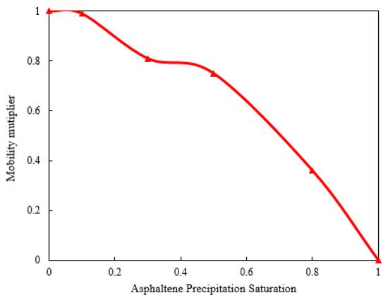
Figure 5.
The relationship between the Asphaltene Precipitation Saturation and the Mobility multiplier.
3. Simulation Setup and Model Validation
In order to further investigate the mechanisms of asphaltene precipitation and deposition during CO2 injection and reveal the impact of asphaltene precipitation on development performance in reservoir exploitation, this study utilized the Petrel integrated simulation platform to construct an asphaltene precipitation model compatible with experimental results. An integrated numerical simulation study was then conducted for CO2 flooding development in heavy oil reservoirs considering asphaltene deposition.
3.1. PVT Fitting
This study used the PVTi module in the phase behavior simulation software ECLIPSE (Version 2021.4) to fit and calculate the PVT experimental data and gas injection swelling experimental data of the crude oil in the Well B area. The fitting work for phase behavior experimental results mainly involves splitting heavy components in crude oil, component aggregation, and fitting the reconstructed component model to saturation pressure, differential liberation experiment data, single flash experiment data, and CO2 injection swelling experiment data. The significance of this approach lies in both improving the speed and accuracy of simulation calculations by reducing the number of components (thereby avoiding non-convergence in simulations) and ensuring that the properties and attributes of the component model remain nearly unchanged before and after recomposition. Through fitting calculations, equation of state (EOS) characteristic parameters capable of characterizing the phase behavior of formation fluids under actual reservoir conditions can be obtained, providing basic data for subsequent component model construction.
- Pseudocomponent Division
Based on parameters such as molecular weight, critical pressure, critical temperature, and critical volume of well stream components, these were grouped into 7 pseudocomponents (original components are shown in Appendix A Table A1, and the recomposed components are shown in Table 3). According to the asphaltene precipitation experimental results above, the C40+ components with appropriate molar mass were classified as asphaltene components.
Table 3.
Composition of Pseudocomponents in Formation Crude Oil after Splitting and Recomposition.
- Constant Composition Expansion Experiment Fitting
The constant composition expansion experiment refers to measuring the relationship between the volume of a fluid sample and pressure under reservoir pressure and temperature conditions with unchanged component composition, thereby obtaining basic phase behavior parameters such as the fluid’s bubble point pressure, relative volume at different pressures, fluid viscosity, density, etc., also simply referred to as PVT relationship testing. Based on the constant composition expansion experiment data, experimental fitting adjustments were performed, with fitting results shown in Figure 6. It can be seen from the figure that the variation law of the relative oil volume of the recomposed components with pressure is almost identical to that of the original components. The fitting error value is 0.5%, indicating a good fitting effect.
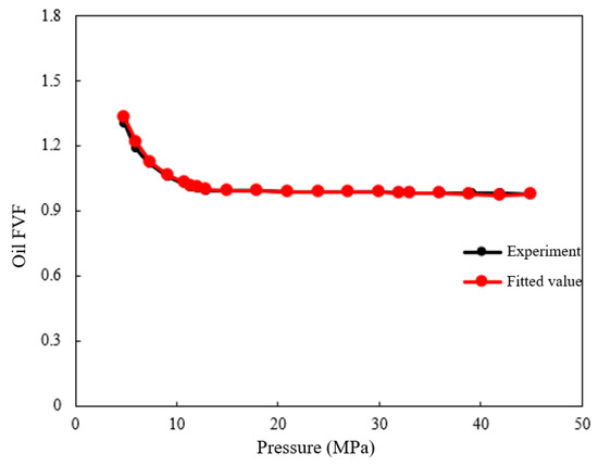
Figure 6.
Constant Composition Expansion Experiment Fitting Curve.
- Differential Liberation (DL) Experiment Fitting
The differential liberation (DL) experiment primarily measures parameters such as crude oil formation volume factor, relative density, crude oil viscosity, gas production volume at different pressures, gas compressibility factor, gas relative density, and natural gas viscosity. Fitting results are shown in Figure 7 and Figure 8, Table 4 and Table 5.
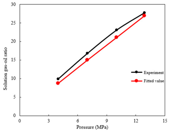
Figure 7.
Solution Gas-Oil Ratio Fitting Curve.
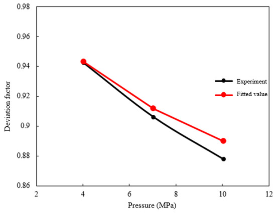
Figure 8.
Deviation Factor Fitting Curve.
Table 4.
Crude Oil Solution Gas-Oil Ratio Fitting.
Table 5.
Crude Oil Deviation Factor Fitting.
As shown in the figures, the solution gas-oil ratio of recomposed components is slightly lower than the value obtained from original component experiments, but the error remains within an acceptable range. The deviation factor shows excellent fitting at low pressures, but as pressure increases, the deviation between fitted and experimental values gradually widens. This issue may arise from inherent deviations in phase equilibrium prediction by the selected Peng-Robinson 3 Parm (PR3) equation of state at high pressures or from the loss of high-pressure phase behavior details due to insufficient pseudocomponent division. Since the error values are within acceptable limits and further adjustment without affecting other fitting results is difficult, the current optimized results are compromisely adopted.
In PVTi data fitting, since the parameters for adjusting viscosity differ from those of other experiments, to avoid mutual interference between fitting results, crude oil viscosity is generally fitted separately after other experimental parameters are completed. In this fitting, the Lohrenz-Bray-Clark (Modified) Formula (1) was used for viscosity calculation. Fitting results are shown in Figure 9a,b. It can be seen from the figures that both crude oil viscosity and gas viscosity exhibit good fitting effects. The fitted values of gas viscosity are slightly lower than the experimental values overall, possibly due to insufficient applicability of the LBC model for specific components or pressure ranges. It may also be caused by the difficulty of measuring high-pressure gas viscosity, potential systematic errors in experimental equipment (such as vibrating string viscometers), or inadequate control of experimental conditions (temperature, pressure). Therefore, further parameter optimization is unnecessary.
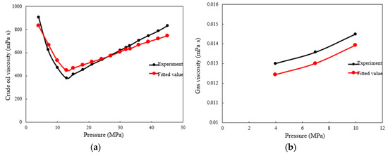
Figure 9.
Viscosity Fitting Results: (a) Crude Oil Viscosity Fitting Curve; (b) Gas Viscosity Fitting Curve.
The calculation expression for viscosity is:
- CO2 Injection Swelling Experiment Fitting
The fitting of the CO2 injection swelling experiment primarily involves adjusting the fluid component model based on the experimental test data of crude oil viscosity under different CO2 injection amounts. Finally, the corresponding experimental fitting comparison is completed as shown in Figure 10, with good fitting results.
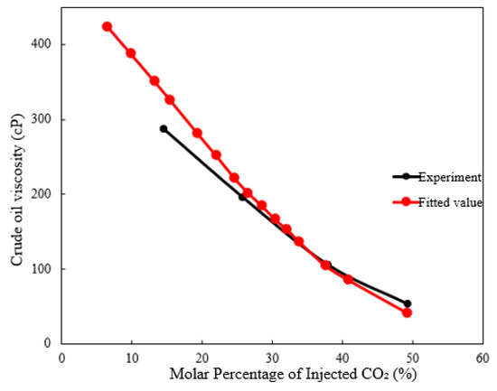
Figure 10.
Swelling Experiment Viscosity Fitting Results.
3.2. Asphaltene Deposition Model
To characterize the impact of asphaltene precipitation on the reservoir during gas injection, this paper uses a three-component model to simulate the process, with all content in this section referenced from the Eclipse Software (Version 2021.4) Manual [34]. The principles of the three-component model are detailed in Appendix B.
Using the experimental results from a series of experiments in Section 2.1, Section 2.2, Section 3 and Section 3.1, the code parameters required for the three-component model are defined. First, the ASPHALTE code is activated, which primarily consists of strings specifying characterization conditions, strings specifying the permeability impairment model, and strings specifying the viscosity model. The characterization condition string defaults to the WIGHT string, with data specified using single-variable codes (ASPP1P, ASPREG) or two-variable codes (ASPPP2P, ASPPW2D). This paper uses single-variable codes, which specify the relationship between pressure and the molar mass percentage of asphaltene dissolved in crude oil: the ASPP1P code designates the corresponding property “pressure,” and the ASPREG code specifies the specific relationship (displayed in a list).
The codes for specifying the permeability impairment model use the three-component model corresponding to SOLIDMMS or SOLIDMMC, which describes solid adsorption caused by changes in fluid mobility. The difference lies in that the two codes correspond to the mobility coefficient and the concentration/saturation of solids adsorbed by the formation, respectively. As the concentration/saturation of solids adsorbed by the formation increases, the mobility coefficient gradually decreases. Since a saturation experiment was conducted in the previous section, the SOLIDMMS code is selected to define the asphaltene model.
The ASPVISO code provides data for modeling oil viscosity changes during asphaltene precipitation. Three models are used to describe viscosity changes:
- Generalized Einstein Model (Single-Parameter): Specifies the slope of relative viscosity as a function of concentration to describe viscosity changes;
- K & D Model (Two-Parameter): Specifies the relationship between mass concentration at maximum packing and intrinsic viscosity to describe viscosity changes;
- Direct Relationship Table: Provides a table of the relationship between the mass fraction of asphaltene precipitate and the oil viscosity multiplier (i.e., the oil viscosity multiplier as a function of the mass fraction of asphaltene precipitate).
After defining all the above codes in combination with the experimental results and PVT fitting results, a unique asphaltene deposition model for the target oil sample in Well Block Xia 018 is formed. However, before using it for numerical simulation, the asphaltene deposition model must first be verified.
Shown as Table 6 is the mapping relationships between model parameters and experimental data.
Table 6.
Mapping relationship between asphaltene code settings and experimental data.
3.3. Model Validation
Core flooding experiments simulate reservoir conditions using field cores to evaluate EOR performance under realistic formation conditions through short- and long-core tests. Optimal injection parameters are determined by varying huff-n-puff parameters, providing guidance for developing similar reservoir exploitation strategies.
During CO2 flooding of crude oil-saturated cores, CO2 reacts with the crude oil, causing asphaltene precipitation that clogs pore throats and increases injection pressure. Based on this phenomenon, this study validated the asphaltene deposition model by conducting CO2 flooding experiments on oil-saturated cores and monitoring changes in injection pressure.
3.3.1. Core Flooding Experiment
Based on a high-temperature and high-pressure core flooding experimental setup, high-purity CO2 was used as the injection medium to conduct core flooding experiments. The experimental process of saturating short cores first and then performing flooding better simulates actual reservoir production processes. This study analyzed pressure evolution at the core scale, gas-injection agent development characteristics, and the distribution pattern of remaining oil.
- Experimental Equipment and Materials
Materials: 200 mL heavy oil sample from Well Block Xia 018; CO2 with a purity of 99.99%; Field cores, etc.
Equipment: Constant-speed and constant-pressure pump: pressure range 0–70 MPa, temperature range ambient—200 °C, flooding rate 0.001–20 mL/min; Core holder: diameter 2.5 cm, length 10 cm; Piston container: volume 1 L, pressure range 0–70 MPa, temperature range ambient—200 °C; High-pressure pipelines: pressure range 0–70 MPa, temperature range ambient—200 °C; Pressure gauge: accuracy 0.01 MPa (as shown in Figure 11).
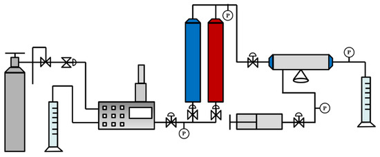
Figure 11.
Core Flooding Experiment Flow.
- Experimental Procedures
- Cores were cleaned, dried, and placed into the core holder, followed by a tightness test. The imbibition method was used to saturate formation water, and the pore volume and porosity of the core assembly were measured;
- The backpressure valve was set to formation pressure, and formation water was used to raise the core pressure to reservoir pressure. Formation water was injected into the short core at a rate of 0.01 mL/min for water saturation. When the pressure stabilized and continuous water production was observed at the outlet, water-phase saturation was considered complete;
- Water was injected into the core through pre-fixed pipelines with a small diameter to generate high pressure. The high-pressure water flow-induced fracturing to achieve the expected effect;
- The core setup was placed in a thermostatic chamber, and dead oil was injected into the core at a rate of 0.01 mL/min for oil saturation. When the pressure stabilized and continuous oil production was observed at the outlet, the core was considered fully oil-saturated. Approximately 2.0 pore volumes (PV) of dead oil were required, and the initial oil saturation of the core was calculated simultaneously;
- CO2 gas was injected into the core at a rate of 0.5 mL/min for CO2 flooding. Each core was flooded for 24 h, with data such as pressure, liquid production, oil production, and gas production recorded every 2 h.
- Experiment Result
As shown in Section 3.3.2 Figure 12, taking Samples 1, 2, and 3 as examples, their injection pressure changes over 24 h were recorded. The figure indicates that the injection pressure remained initially stable; as injection time increased, it began to rise around 10 h, peaked at approximately 15 h, and finally dropped rapidly to a constant value. This behavior is attributed to the following: when CO2 is injected, it first destabilizes asphaltene components, causing asphaltene precipitation that partially clogs pore throats, leading to a rapid increase in injection pressure. As the injection pressure further increases, CO2 becomes miscible with the crude oil, increasing asphaltene solubility and unclogging the blocked pore throats, causing the injection pressure to quickly return to a normal level. However, due to the irreversibility of the damage, the injection pressure after unclogging remains slightly higher than before the clogging occurred.
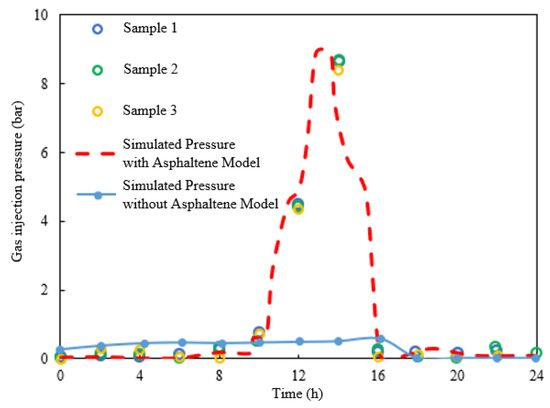
Figure 12.
Comparison of Injection Pressure Changes During Flooding Between Simulation and Experimental Records.
3.3.2. Core Flooding Numerical Simulation
After successfully establishing the asphaltene deposition model, the calibrated fluid composition model was imported into Petrel, forming an integrated numerical simulation technology that accounts for the coupling of multiple physicochemical processes such as asphaltene precipitation and migration. Before applying this technology, the accuracy of the model was first validated.
A core-scale mechanistic model matching the cores used in the flooding experiments was built using the Petrel platform. The model was parameterized with physical property data from the core samples, including average permeability, average porosity, and dimensions (length and diameter). The final properties of the mechanistic model were determined as follows: total length 6 cm, diameter 2.5 cm, porosity 0.2, permeability 100 mD, and grid size 25 mm × 25 mm × 1 mm.
The established mechanistic model is shown in Figure 13. To avoid convergence issues, reduce computation time, and simplify the calculation process, a 1D (stratified only in the k-direction) rectangular mechanistic model was used for simplification. The core-scale model was vertically divided into 60 layers, with three horizontal wells evenly spaced at the bottom—each equipped with 3 uniform perforation clusters—serving as CO2 injection wells to simulate the gas injection end of the core flooding experiment. At the top, nine production wells with uniform spacing were used for oil production, simulating the fluid outlet end of the experiment. The pre-imported and calibrated composition model was applied to the defined simulation scheme, and asphaltene deposition codes were added to activate the asphaltene deposition model. To match the actual gas injection rate and flooding time in the experiments, the numerical simulation was set with a constant injection rate of 0.5 mL/min for 24 h, recording results every 1 h. After configuration, the simulation scheme was run. The flooding results are shown in Figure 14.
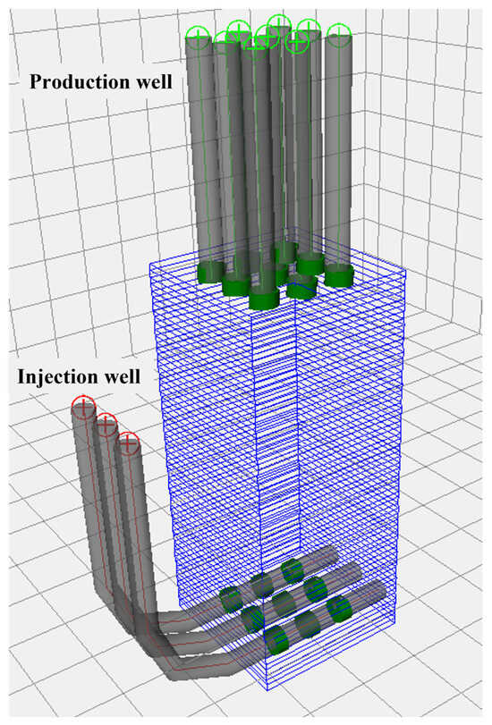
Figure 13.
1D Core-Scale Mechanistic Model.
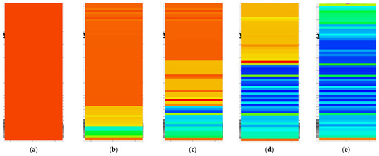
Figure 14.
Core Flooding Simulation Process (Taking Oil Saturation as an Example): Flooding Effect at (a) 1 h; (b) 4 h; (c) 8 h; (d) 12 h; (e) 16 h.
As shown in Figure 12, as the flooding simulation progresses, CO2 injected from the bottom displaces crude oil upward throughout the core, corresponding to a decrease in oil saturation starting from the lower part of the core. After 16 h of flooding, oil saturation stabilizes, indicating most of the crude oil in the core model has been displaced. During the simulation, uneven oil saturation distribution occurs in the middle section of the core model, likely due to asphaltene deposition—initially treated as a solid phase (unrecognized by oil saturation properties)—reverting to a free asphaltene state (recognized as a liquid component by oil saturation properties) due to the unclogging effect. Additionally, a comparison of injection pressure between the flooding experiment and core flooding simulation is shown in Figure 12. The figure demonstrates that simulation results without considering the asphaltene deposition model exhibit significant discrepancies with experimental data, whereas results incorporating the asphaltene deposition model show good agreement with experimental results. This preliminarily validates the effectiveness of the asphaltene deposition model.
4. Field Applications
Based on the previous descriptions of the block’s formation and oil sample characteristics, the crude oil in Well Block Xia 018 exhibits high viscosity and poor reservoir physical properties. The field plans to enhance production in Well Y through reservoir fracturing stimulation. Determining multiple construction and production parameters for reservoir fracturing requires integrating a reservoir mechanistic model with actual fracturing pumping schedules. Therefore, this chapter establishes a numerical simulation model that incorporates both the compositional model and asphaltene deposition model, conducting a systematic study on parameter optimization and screening. Based on this, optimal construction and production parameters are selected, and preliminary production recommendations are provided.
4.1. Mechanistic Model Development
To simplify calculations, demonstrate the workflow, and eliminate the influence of formation property heterogeneity, this chapter uses a computationally efficient mechanistic model for the study.
Based on the location of the target horizontal well Y, suitable regional size and thickness were defined to form a rectangular block measuring 1600 m × 900 m × 50 m, with a grid size of 20 m × 20 m × 5 m and a total of 36,520 grids. Property modeling for the mechanistic model was referenced from the geological data provided by the field, using average values. Key properties required for fracturing simulation and subsequent production simulation include porosity, permeability, water saturation, oil saturation, and geomechanical parameters (Poisson’s ratio, Young’s modulus, maximum and minimum horizontal principal stresses, overburden pressure, pore pressure, etc.), as listed in Table 7.
Table 7.
Key Parameters of Reservoir Mechanistic Model for Well Y in Xia 018 Well Block.
The established mechanistic model is shown in Figure 15, where Well Y is depicted as a horizontal well, preparing for the creation of zonesets in subsequent fracturing simulations.
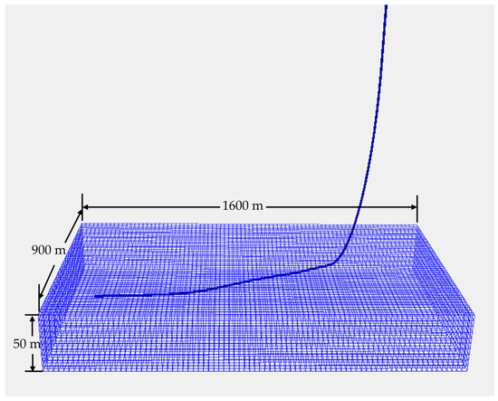
Figure 15.
Reservoir Mechanistic Model for Well Y in Xia 018 Well Block.
4.2. Fracturing and Production Optimization
Both fracturing operations and production prediction simulations require determining numerous parameters, whose selection ranges are primarily based on field data combined with operational experience. Under normal conditions, the fracturing parameters to be optimized include cluster spacing, fracturing stage length, fluid volume, proppant volume, CO2 injection volume, injection rate, well spacing, etc.; production regime parameters include daily oil (gas) production and production time. Since Well Y already has existing perforation data, cluster spacing will not be adjusted in this optimization.
Given the large number of fracturing parameters to optimize, an orthogonal array design was chosen to ensure uniform dispersion of parameters and minimize the number of experiments while enabling main effect analysis. The fracturing parameters consist of 5 factors with 4 levels each and 1 factor with 5 levels (well spacing), which cannot be directly accommodated by standard orthogonal arrays. Instead, the pseudo-level method was applied: using the standard orthogonal table L16(45) (16 experiments for 5 factors with 4 levels), the 6th factor (well spacing, 5 levels) was integrated into the table through pseudo-level adjustment, forming L20(45 × 51) to maintain orthogonality of main effects. For details, the designed experimental schemes are listed in Appendix A2. The final optimized fracturing parameters are fracturing stage length of 1000 m, fluid volume per stage of 100 m3, proppant volume per stage of 100 m3, CO2 injection volume per stage of 110 m3, injection rate of 14 m3/min, and well spacing of 260 m.
After optimizing fracturing parameters with SRV (Stimulated Reservoir Volume) as the target, the selected parameter set was further used to optimize production regimes with cumulative oil production as the objective.
Production simulation results (Figure 16, Figure 17, Figure 18 and Figure 19) show that as daily oil production increases, cumulative oil production rises gradually, while stable production time decreases and the pressure depletion radius in the well block expands. Since stable production cannot be sustained, increasing daily production beyond 15 m3/d leads to negligible growth in total production; thus, 15 m3/d is selected as the optimal daily oil production rate. As production years increase, pressure contours at the end of each period indicate an expanding depletion area. While cumulative oil production continues to grow, the average annual oil production declines progressively. Comprehensively considering input costs and economic benefits, 15 years is determined as the optimal production time.
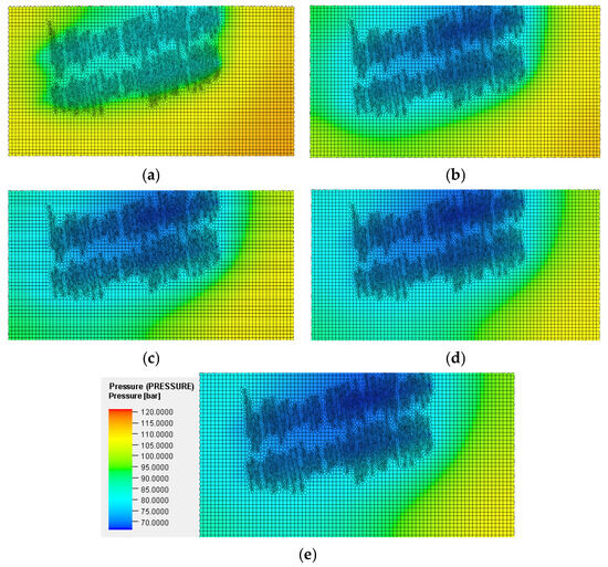
Figure 16.
Pressure Contours of the Well Block at the End of 10 Years under Different Daily Oil Production Rates: (a) 9 m3/d; (b) 12 m3/d; (c) 15 m3/d; (d) 18 m3/d; (e) 21 m3/d.
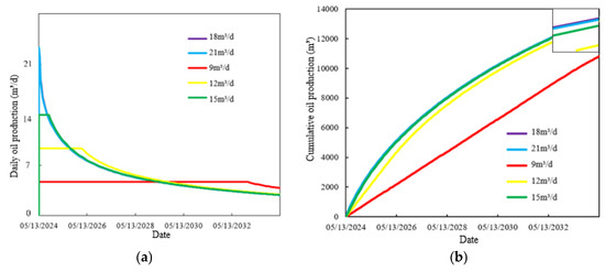
Figure 17.
Variations in Daily Oil Production over Time under Different Daily Oil Production Rate Settings: (a) variations in daily oil production over time; (b) variations in cumulative oil production over time.
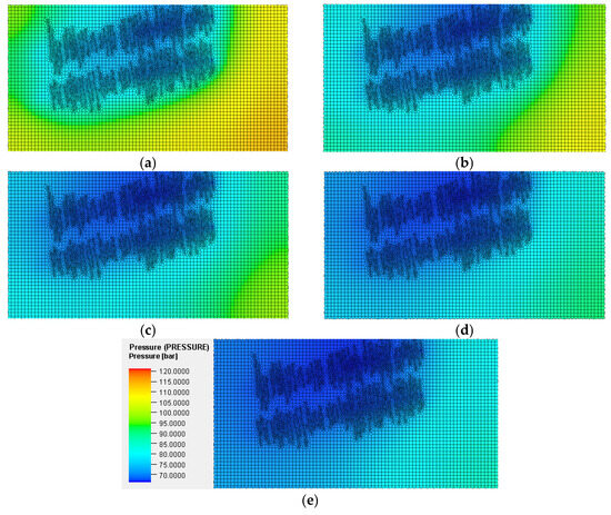
Figure 18.
Pressure Contours of the Well Block at the End of Different Production Years: (a) 5 years; (b) 10 years; (c) 15 years; (d) 20 years; (e) 25 years.
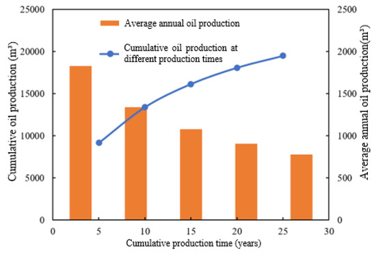
Figure 19.
Variations in Cumulative Oil Production and Average Annual Oil Production Under Different Production Time Settings.
4.3. Case Well Production Simulation
Using the production regime optimized in Section 4.2, a constant-production-rate prediction simulation was conducted for Well Y with a set daily production rate of 15 m3/day and a production duration of 15 years. The code for the asphaltene deposition model was activated during the simulation, and the results are shown in Figure 20. As indicated in the figure, with the progression of the production simulation, CO2 in the fracturing fluid reacts with heavy oil in the formation, causing asphaltene deposition in the wellbore vicinity. This leads to a decrease in reservoir permeability and the formation of local abnormal high pressure in the near-wellbore region, as shown in Figure 20b,c. However, as the simulation proceeds, the local abnormal high pressure gradually decreases. It is inferred that the increased pressure promotes miscibility between CO2 and asphaltene, enhancing asphaltene solubility and causing partial debottlenecking. Nevertheless, the reduced reservoir permeability cannot fully recover—by the end of 2039 (the final production stage), the pressure in the near-wellbore region remains slightly higher than in other areas, as shown in Figure 20d.
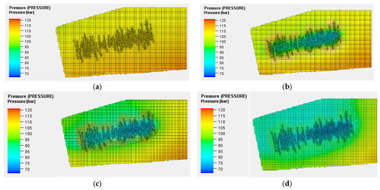
Figure 20.
Variations in Pressure Contour Plot for production prediction of Well Y: (a) The end of 2024; (b) The end of 2026; (c) The end of 2029; (d) The end of 2039.
A comparative simulation without activating the asphaltene deposition model was also performed, with results compared in Figure 21 and Figure 22. Without the asphaltene model (which does not account for asphaltene-induced damage), reservoir permeability remains unchanged, and the simulated curves for daily oil production, bottomhole flowing pressure, and cumulative oil production follow normal constant-production-rate trends. When the asphaltene deposition model is activated, bottomhole flowing pressure decreases more slowly, and daily production declines due to simulated permeability damage from asphaltene. Asphaltene plugging reaches its maximum severity by mid-2026, after which debottlenecking occurs and bottomhole pressure decreases. However, due to the irreversibility of permeability reduction (modeled by setting the flocculation rate higher than the dissolution rate in the asphaltene deposition model), bottomhole pressure remains slightly higher than in the non-asphaltene model scenario. Daily production is also lower than the non-asphaltene case, resulting in lower cumulative production: the standard scenario yields 13,000 m3, while the asphaltene-inclusive scenario yields 11,700 m3. For field production guidance, periodic debottlenecking operations may be required between 2026 and 2029 to maintain stable well productivity and improve ultimate recovery. From 2029 to 2039, the dosage and frequency of debottlenecking agents can be reduced.
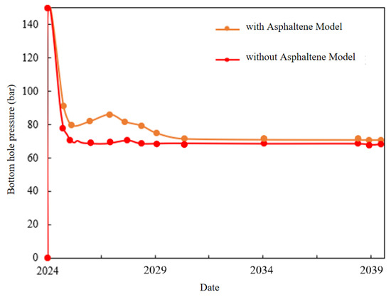
Figure 21.
Bottom hole Pressure of Well Y after 15 years of production.
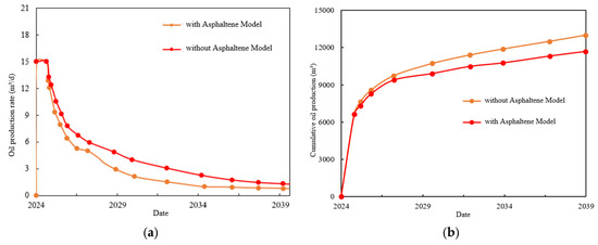
Figure 22.
Oil Production Rate and Cumulative Oil Production of Well Y after 15 years of production: (a) Oil Production Rate of Well Y after 15 years of production; (b) Cumulative Oil Production of Well Y after 15 years of production.
5. Conclusions
This study addresses the challenges of production enhancement in heavy oil reservoirs and damage caused by asphaltene deposition. Adopting a technical approach comprising “mechanism experiments—model development—parameter optimization—field validation,” it investigates the reaction mechanisms of CO2 injection into oil samples from the target block. Component and asphaltene deposition models specific to the oil samples were developed, with the accuracy of the asphaltene deposition model validated through core flooding experiments and numerical simulations. Fracturing and production parameters for the target area were optimized and successfully applied in field operations, leading to the following key findings:
- This study reveals the duality of the interaction mechanism between CO2 and heavy oil. Experiments confirm that CO2 reduces heavy oil viscosity through molecular diffusion and expands crude oil volume, significantly enhancing fluidity. However, CO2 dissolution disrupts the resin-asphaltene equilibrium: asphaltene precipitation is triggered when pressure drops below 25.6 MPa, reaching a peak of 2% at 16 MPa. Controlling the pre-injected CO2 volume in parameter optimization is essential to avoid reducing fracture conductivity.
- A research approach integrating the asphaltene deposition model into a unified simulation was proposed. PVT parameters were fitted using experimental data and the ECLIPSE-PVTi module. An asphaltene code was defined and applied to construct a three-component asphaltene deposition model, with its reliability validated through dual verification of core flooding experiments and numerical simulation. Enabling the asphaltene model in subsequent unified simulation cases improved prediction accuracy, demonstrating significant practical value;
- Collaborative optimization of fracturing operation parameters is completed. Based on the established orthogonal array, the highest unit-length Stimulated Reservoir Volume (SRV) was achieved at a fracturing stage length of 1000 m. Combining economic evaluation, the optimal parameter combination was determined as: fluid volume per stage of 1000 m3, proppant volume of 1000 m3, and injection rate of 14 m3/min. A design framework for similar reservoirs is provided;
- Conducted production simulation and prediction for case wells using optimized fracturing parameters and production regimes, integrated with the validated component and asphaltene models. A 3D geomechanical model was built for Well Y in the Xia 018 block, and simulations were performed using the optimized parameters. Compared with the scenario without the asphaltene deposition model, the 15-year predicted cumulative oil production was 1.17 × 10⁴ m3, a 10% decrease. Pressure contour plots of the well area revealed that the combined effect of declining pore pressure and CO2 during production would induce asphaltene precipitation in the near-well region. These results guide planning debottlenecking timing in field operations, demonstrating significant practical significance.
Author Contributions
Conceptualization, X.G. (Xiding Gao) and T.Z.; methodology, X.G. (Xiding Gao); software, L.Q.; validation, X.G. (Xiding Gao) and L.Q.; formal analysis, L.Z.; investigation, W.S.; resources, W.S.; data curation, X.G. (Xin Guan); writing—original draft preparation, X.G. (Xiding Gao); writing—review and editing, T.Z.; visualization, X.G. (Xin Guan); supervision, T.Z.; project administration, T.Z. All authors have read and agreed to the published version of the manuscript.
Funding
This research received no external funding.
Data Availability Statement
The original contributions presented in this study are included in the article. Further inquiries can be directed to the corresponding author.
Conflicts of Interest
The authors declare no conflicts of interest.
Appendix A
Appendix A.1
Table A1.
Well Stream Composition Data.
Table A1.
Well Stream Composition Data.
| Composition | Flash Oil Composition | Flash Gas Composition | Composition | ||
|---|---|---|---|---|---|
| (mol%) | (wt%) | (mol%) | (mol%) | (wt%) | |
| H2S | 0.00 | 0.00 | 0.00 | 0.00 | 0.00 |
| N2 | 0.00 | 0.00 | 0.00 | 0.00 | 0.00 |
| CO2 | 0.00 | 0.00 | 0.00 | 0.00 | 0.00 |
| C1 | 0.00 | 0.00 | 97.96 | 29.16 | 1.91 |
| C2 | 0.00 | 0.00 | 0.89 | 0.26 | 0.03 |
| C3 | 0.00 | 0.00 | 0.61 | 0.18 | 0.03 |
| iC4 | 0.00 | 0.00 | 0.13 | 0.04 | 0.01 |
| nC4 | 0.00 | 0.00 | 0.27 | 0.08 | 0.02 |
| iC5 | 0.00 | 0.00 | 0.08 | 0.02 | 0.01 |
| nC5 | 0.00 | 0.00 | 0.06 | 0.02 | 0.01 |
| C6 | 5.93 | 1.46 | 0.00 | 4.16 | 1.43 |
| C7 | 1.64 | 0.46 | 0.00 | 1.15 | 0.45 |
| C8 | 1.21 | 0.38 | 0.00 | 0.85 | 0.37 |
| C9 | 1.61 | 0.57 | 0.00 | 1.13 | 0.56 |
| C10 | 2.18 | 0.86 | 0.00 | 1.53 | 0.84 |
| C11 | 2.80 | 1.21 | 0.00 | 1.97 | 1.18 |
| C12 | 3.73 | 1.76 | 0.00 | 2.62 | 1.73 |
| C13 | 4.89 | 2.51 | 0.00 | 3.43 | 2.46 |
| C14 | 5.10 | 2.84 | 0.00 | 3.58 | 2.78 |
| C15 | 5.26 | 3.17 | 0.00 | 3.69 | 3.11 |
| C16 | 4.88 | 3.17 | 0.00 | 3.43 | 3.11 |
| C17 | 5.44 | 3.78 | 0.00 | 3.82 | 3.70 |
| C18 | 3.47 | 2.55 | 0.00 | 2.44 | 2.51 |
| C19 | 2.86 | 2.21 | 0.00 | 2.01 | 2.16 |
| C20 | 2.83 | 2.28 | 0.00 | 1.99 | 2.24 |
| C21 | 2.44 | 2.08 | 0.00 | 1.71 | 2.04 |
| C22 | 2.18 | 1.95 | 0.00 | 1.53 | 1.91 |
| C23 | 2.09 | 1.95 | 0.00 | 1.47 | 1.91 |
| C24 | 2.03 | 1.97 | 0.00 | 1.42 | 1.92 |
| C25 | 2.21 | 2.24 | 0.00 | 1.55 | 2.19 |
| C26 | 2.40 | 2.52 | 0.00 | 1.68 | 2.47 |
| C27 | 2.87 | 3.14 | 0.00 | 2.01 | 3.07 |
| C28 | 2.75 | 3.13 | 0.00 | 1.93 | 3.06 |
| C29 | 2.73 | 3.22 | 0.00 | 1.92 | 3.16 |
| C30 | 2.12 | 2.59 | 0.00 | 1.49 | 2.54 |
| C31 | 1.76 | 2.22 | 0.00 | 1.24 | 2.18 |
| C32 | 1.34 | 1.75 | 0.00 | 0.94 | 1.71 |
| C33 | 1.25 | 1.68 | 0.00 | 0.88 | 1.65 |
| C34 | 1.22 | 1.68 | 0.00 | 0.85 | 1.64 |
| C35 | 1.26 | 1.79 | 0.00 | 0.88 | 1.75 |
| C36+ | 15.52 | 36.89 | 0.00 | 10.90 | 36.16 |
| Total | 100.00 | 100.00 | 100.00 | 100.00 | 100.00 |
| molecular weight of C36+, 811 | |||||
| density of C36+, 0.9885 g/cm3 | |||||
Appendix A.2
Table A2.
Orthogonal Experimental Table for Fracturing Parameters.
Table A2.
Orthogonal Experimental Table for Fracturing Parameters.
| Case | Fracturing Length (m) | Single Stage Fluid Volume (m3) | Fracturing Length (m) | Single Stage Fluid Volume (m3) | Fracturing Length (m) | Single Stage Fluid Volume (m) |
|---|---|---|---|---|---|---|
| 1 | 600 | 600 | 600 | 90 | 10 | 200 |
| 2 | 600 | 800 | 800 | 100 | 12 | 225 |
| 3 | 600 | 1000 | 1000 | 110 | 14 | 250 |
| 4 | 600 | 1200 | 1200 | 120 | 16 | 260 |
| 5 | 600 | 600 | 600 | 90 | 10 | 275 |
| 6 | 800 | 600 | 800 | 100 | 14 | 250 |
| 7 | 800 | 800 | 1000 | 120 | 16 | 275 |
| 8 | 800 | 1000 | 1200 | 90 | 10 | 225 |
| 9 | 800 | 1200 | 600 | 110 | 12 | 260 |
| 10 | 800 | 600 | 800 | 120 | 14 | 200 |
| 11 | 1000 | 600 | 1000 | 90 | 16 | 260 |
| 12 | 1000 | 800 | 1200 | 100 | 10 | 275 |
| 13 | 1000 | 1000 | 600 | 110 | 12 | 200 |
| 14 | 1000 | 1200 | 800 | 120 | 14 | 225 |
| 15 | 1000 | 600 | 1000 | 90 | 16 | 250 |
| 16 | 1200 | 600 | 1200 | 100 | 12 | 260 |
| 17 | 1200 | 600 | 600 | 110 | 14 | 275 |
| 18 | 1200 | 1000 | 800 | 120 | 16 | 200 |
| 19 | 1200 | 1200 | 1000 | 90 | 10 | 225 |
| 20 | 1200 | 600 | 1200 | 100 | 12 | 250 |
This table ensures that each level of the 4-level factors appears 5 times, and each level of the 5-level factor (well spacing) appears 4 times. For any two 4-level factors, their level combinations occur at least once, and combinations between 4-level and 5-level factors cover over 80% of possible pairings.
Due to the numerous factors affecting the horizontal well fracturing construction of SRV, the fracturing length was first optimized based on the SRV magnitude of each simulation scheme, as shown in Figure A1. The simulation schemes for different horizontal section fracturing lengths were averaged, and the average SRV values for different lengths are shown in Figure A2. It can be seen from the figures that the single-well SRV increases with the increase of horizontal section fracturing length, while the SRV per unit fracturing length decreases with the increase of horizontal section fracturing length. Therefore, the intersection point of the two curves, i.e., the horizontal fracturing section length of 1000 m, was selected as the optimal fracturing section length.
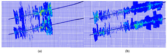
Figure A1.
Comparison of Fracture Distribution under Different Horizontal Fracturing Section Length Schemes: (a) case 3–600 m; (b) case 17–1200 m.
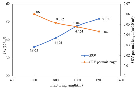
Figure A2.
Relationship between Single-Well SRV and SRV per Unit Length under Different Fracturing Section Length Schemes.
When the well spacing is less than 250 m, all pumping program schemes carry the risk of fracturing crossflow. When the well spacing is 260 m or 270 m, some schemes avoid crossflow. Considering the well area trends east-west with shorter north-south spacing, and Well Y is approximately 400 m from the northern reservoir boundary, a well spacing of 270 m would place wells north of Well Y too close to the boundary, preventing effective utilization of the pressure relief area. Therefore, 260 m is selected as the optimal well spacing after comprehensive consideration. As shown in Figure A3.
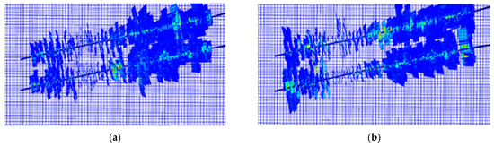
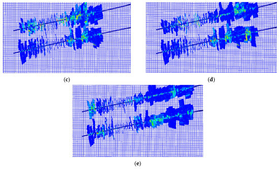
Figure A3.
Schematic of Simulation Results for Fracturing Schemes under Different Well Spacings: (a) 200 m; (b) 225 m; (c) 250 m; (d) 260 m; (e) 275 m.
As shown in Figure A4: with the increase of fluid volume per stage in the pumping program, the fracture length and single-well SRV generally show an increasing trend. However, when the fluid volume exceeds 1000 m3, the growth rate of fracture length and SRV significantly decreases. Considering comprehensive factors such as field construction costs, the optimal fluid volume per stage is determined to be 1000 m3.
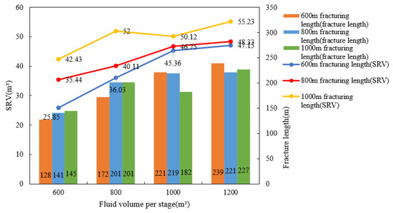
Figure A4.
Variations of SRV and Fracture Length under Different Fluid Volume Schemes.
Similarly, the optimal parameters for sand volume, CO2 injection volume, displacement rate, etc., were determined by the same optimization approach.
Appendix B
From a molecular dynamics perspective, the mechanism by which CO2 injection into heavy oil induces asphaltene precipitation can be summarized into three key processes, validated by both molecular dynamics (MD) simulations and experiments:
- Disruption of Asphaltene Micelles by CO2;
CO2 molecules diffuse into asphaltene micelles, gradually extracting non-polar and lightly polar components (e.g., saturates, aromatics), leading to micelle disintegration. MD simulations show that asphaltene micelles undergo a two-step precipitation process in a CO2 environment: first forming tetramers or dimers, which then aggregate further via π-π stacking and finally adsorb onto rock surfaces (e.g., silica) to form irreversible deposits. This process aligns with experimental observations of increased asphaltene interlayer spacing and reduced aggregation rates [35,36].
- 2.
- Reconstruction of Intermolecular Interactions;
CO2 alters intermolecular interactions: its π-π stacking with asphaltene aromatic rings enhances charge transfer, while dipole effects strengthen hydrogen bonding in polar groups, destabilizing aggregates. Supercritical CO2’s high permeability further weakens asphaltene-resin interactions [37,38].
- 3.
- Influence of Thermodynamic Conditions;
Thermodynamically, increased pressure enhances CO2-asphaltene binding to grow aggregate sizes, while lower temperatures boost CO2 solubility and reduce asphaltene thermal motion, favoring π-π stacking and precipitation [39].
The three-component model accounts for six potential behavioral characteristics of asphaltene during CO2 injection, including precipitation, dissolution, flocculation, dissociation, deposition, and entrainment. Specifically: Precipitation refers to the formation of asphaltene fine particles (“fines”) in the fluid; Dissolution (the reverse of precipitation) refers to the redissolution of these fines into the oil; Flocculation is the aggregation of precipitated fines into larger particles (flocs), as shown in Figure A5; Dissociation (the reverse of flocculation) is the breakup of flocs into fines; Deposition refers to flocs leaving the fluid and adhering to reservoir rock surfaces; Entrainment (the reverse of deposition) is the resuspension of deposited asphaltene into the fluid.
The three components interconvert in the fluid, with asphaltene formation simulated by defining the interconversion rates of precipitation, flocculation, and deposition. The corresponding calculation formulas for the precipitation-dissolution, flocculation-dissociation, and deposition-entrainment processes are provided in Equations (A1)–(A3), respectively:
Figure A5.
Schematic diagram of Asphaltene Flocculation Mechanism.
In Equation (A1), xlim represents the limiting mole fraction of the precipitated component dissolved in oil; Wlim denotes the maximum amount of dissolvable asphaltene; M is the molecular weight of crude oil; and mwp is the molecular weight of the precipitated component. In Equation (A2), Rf is the rate of fines converting to flocculated components (flocculation reaction); V is the fluid volume; Vp is the pore volume; SS is the solid saturation, representing the fractional pore volume filled by asphaltene deposition; Cf is the fines concentration in the oil phase; So is the oil saturation; Bo is the molar density of crude oil; and rf is the code-specified flocculation rate. In Equation (A3), Rd represents the deposition reaction rate; α is the code-specified adsorption coefficient; Cfloc is the flocculated component concentration in the oil phase; γ2 is the code-specified blockage coefficient; v is the average oil flow velocity; L is the length of oil flow; and Cfcr is the code-specified critical floc concentration for blockage initiation.
In the dissociation reaction, the conversion of flocculated components to fines occurs at a rate given by Equation (A4):
In the equation, represents the concentration of flocs in the oil phase; xf is the mole fraction of flocs in the oil phase; rdis is the code-specified dissociation rate; deposition and entrainment of asphaltene are modeled using solid components. Deposition is simulated through a pair of reactions between asphaltene floc components and deposited asphaltene components (Equation (A3)). Blockage occurs only when the floc concentration exceeds the critical floc concentration (Cf > Cfcr) and the volume fraction of deposited asphaltene (represented by solid saturation Ss) exceeds the critical value (Ss ≥ Scr), where Cfcr and Scr are specified by the ASPLCRT code—a code used to control asphaltene blockage.
The reverse reaction of Equation (A3) is the entrainment reaction, where deposited asphaltene converts to floc components at a rate given by Equation (A5):
In the equation, β represents the entrainment coefficient; Ucr is the critical entrainment velocity.
Both the average oil flow rate and average oil velocity are calculated in the previous time step. First, the total oil flow rates (Fox, Foy, Foz) and flow areas (Ax, Ay, Az) in each direction are computed by summing the flow rates and areas over opposite faces, including any contributions from non-adjacent connections, as shown in Equations (A6) and (A7):
Flow rates are calculated here based on the inter-grid transmissibility T, pressure difference (Δp), relative permeability of oil in the grid cell (kro), and crude oil viscosity (μo). The average velocity in each direction is given by Equation (A8):
The average flow is determined by taking the average over the N dimensions, as Equation (A9):
The phase average velocity is calculated using the root mean square of the direction velocities, as Equation (A10):
where ϕ is the porosity; C is a conversion factor that is used to convert volumes from reservoir barrels to cubic feet if the simulation is in field units. These flow and velocity calculations only take into account the flows between grid blocks.
References
- Cho, J.; Kim, T.H.; Chang, N.; Lee, K.S. Effects of asphaltene deposition-derived formation damage on three-phase hysteretic models for prediction of coupled CO2 enhanced oil recovery and storage performance. J. Pet. Sci. Eng. 2019, 172, 988–997. [Google Scholar] [CrossRef]
- Ettehadtavakkol, A.; Lake, L.W.; Bryant, S.L. CO2-EOR and storage design optimization. Int. J. Greenh. Gas Control 2014, 25, 79–92. [Google Scholar] [CrossRef]
- Zou, C.; Xue, H.; Xiong, B.; Zhang, G.; Pan, S.; Jia, C.; Wang, Y.; Ma, F.; Sun, Q.; Guan, C.; et al. Connotation, innovation and vision of “carbon neutral”. Nat. Gas Ind. 2021, 41, 46–57. [Google Scholar]
- Shuhui, Z.; Jun, W.; Yan, L. Development of China’s natural gas industry during the 14th Five-Year Plan in the background of carbon neutrality. Nat. Gas Ind. 2021, 41, 171–182. [Google Scholar]
- Mehdi, S.; Raoof, G.; Ebrahim, K.; Majid, M. Temperature profile estimation: A study on the Boberg and Lantz steam stimulation model. Petroleum 2020, 6, 92–97. [Google Scholar]
- Guo, Q.; Wu, N.; Yan, W.; Chen, N. An assessment method for deep gas resources. Acta Pet. Sin. 2019, 40, 383–394. [Google Scholar]
- Wang, H.; Li, G.; Shen, Z. Feasibility Analysis on Shale Gas Exploitation with Supercritical CO2. Pet. Drill. Tech. 2011, 39, 30–35. [Google Scholar]
- Shen, Z.; Wang, H.; Li, G. Feasibility analysis of coiled tubing drilling with supercritical carbon dioxide. Pet. Explor. Dev. 2010, 37, 743–747. [Google Scholar] [CrossRef]
- Cheng, Y.; Li, G.; Wang, H.; Tian, S.; Zhang, Y. feasibility analysis on coiled-tubing jet fracturing with supercritical CO2. Oil Drill. Prod. Technol. 2013, 35, 73–77. [Google Scholar]
- Liu, H.; Wang, F.; Zhang, J.; Meng, S.; Duan, Y. Fracturing with carbon dioxide: Application status and development trend. Pet. Explor. Dev. 2014, 41, 466–472. [Google Scholar] [CrossRef]
- Wang, H.; Li, G.; Shen, Z.; Song, X.; Cao, Y. Supercritical carbon dioxide drilling and the development of future drilling technology. Spec. Oil Gas Reserv. 2013, 19, 1–5. [Google Scholar]
- Demiral, B.; Khanifar, A.; Darman, N.B.; Alian, S.S. Study of Asphaltene Precipitation and Deposition Phenomenon during WAG Application. In Proceedings of the SPE Enhanced Oil Recovery Conference, Kuala Lumpur, Malaysia, 19–21 July 2015. [Google Scholar]
- Alvarado, V.; Moradi, M.; Wang, X. Role of Acid Components and Asphaltenes in Wyoming Water-in-Crude Oil Emulsions. Energy Fuels 2011, 25, 4606–4613. [Google Scholar] [CrossRef]
- Shen, Z.; Sheng, J. Experimental study of permeability reduction and pore size distribution change due to asphaltene deposition during CO2 huff and puff injection in Eagle Ford shale. Asia-Pac. J. Chem. Eng. 2017, 12, 381–390. [Google Scholar] [CrossRef]
- Currier, R.P.; Viswanathan, H.S.; Porter, M.L.; Kang, Q.; Middleton, R.S.; Jiménez-Martínez, J.; Hyman, J.D.; Carey, J.W.; Karra, S. Shale gas and non-aqueous fracturing fluids: Opportunities and challenges for supercritical CO2. Appl. Energy 2015, 147, 500–509. [Google Scholar] [CrossRef]
- Raha, S.; Maqbool, T.; Fogler, H.S.; Hoepfner, M.P. Modeling the Aggregation of Asphaltene Nanoaggregates in Crude Oil−Precipitant Systems. Energy Fuels 2011, 25, 1585–1596. [Google Scholar] [CrossRef]
- Miri, R.; Zendehboudi, S.; Kord, S.; Vargas, F.; Lohi, A.; Elkamel, A.; Chatzis, I. Experimental and numerical modeling study of gravity drainage considering asphaltene deposition. Ind. Eng. Chem. Res. 2014, 53, 11512–11526. [Google Scholar] [CrossRef]
- Vargas, F.M.; Garcia-Bermudes, M.; Boggara, M.; Punnapala, S.; Abutaqiya, M.; Mathew, N.; Prasad, S.; Khaleel, A.; Al Rashed, M.; Al Asafen, H. On the Development of an Enhanced Method to Predict Asphaltene Precipitation. In Proceedings of the Offshore Technology Conference, Houston, TX, USA, 5–8 May 2014. [Google Scholar] [CrossRef]
- AlHammadi, A.A.; Chen, Y.; Yen, A.; Wang, J.; Creek, J.L.; Vargas, F.M.; Chapman, W.G. Effect of the gas composition and gas/oil ratio on asphaltene deposition. Energy Fuels 2017, 31, 3610–3619. [Google Scholar] [CrossRef]
- Li, Z.; Firoozabadi, A. Modeling asphaltene precipitation by n-alkanes from heavy oils and bitumens using cubic-plus-association equation of state. Energy Fuels 2010, 24, 1106–1113. [Google Scholar] [CrossRef]
- Hawthorne, S.B.; Gorecki, C.D.; Sorensen, J.A.; Steadman, E.N.; Harju, J.A.; Melzer, S. Hydrocarbon mobilization mechanisms from upper, middle, and lower Bakken reservoir rocks exposed to CO2 SPE. In Proceedings of the Unconventional Resources Conference Canada, Society of Petroleum Engineers, Calgary, AB, Canada, 5–7 November 2013. [Google Scholar]
- Yu, W.; Lashgari, H.R.; Wu, K.; Sepehrnoori, K. CO2 injection for enhanced oil recovery in Bakken tight oil reservoirs. Fuel 2015, 159, 354–363. [Google Scholar] [CrossRef]
- Wu, R.; Wei, B.; Zou, P.; Zhang, X.; Jing, S.; Gao, K. Effect of Supercritical CO2 on the Physical Properties of Conventional Heavy Oil and Extra-heavy Oil. Oilfield Chem. 2018, 35, 440–446. [Google Scholar]
- Mehdi, M.; Ali, A.R.; Rohaldin, M. Microfluidic experiments and numerical modeling of pore-scale Asphaltene deposition: Insights and predictive capabilities. Energy 2023, 283, 129210. [Google Scholar]
- Alimohammadi, S.; Zendehboudi, S.; James, L. A comprehensive review of asphaltene deposition in petroleum reservoirs: Theory, challenges, and tips. Fuel 2019, 252, 753–791. [Google Scholar] [CrossRef]
- Zhang, H.; Huang, Q.; Zhang, D.; Lyu, Y.; Wang, Q.; Li, R.; Zhang, F.; Liu, L.; Xue, H. Experimental and molecular dynamics simulation investigations of adhesion in heavy oil/water/pipeline wall systems during cold transportation. Energy 2022, 250, 123811. [Google Scholar] [CrossRef]
- Sadeghi Yamchi, H.; Zirrahi, M.; Hassanzadeh, H.; Abedi, J. Numerical simulation of asphaltene deposition in porous media induced by solvent injection. Int. J. Heat Mass Transf. 2021, 181, 121889. [Google Scholar] [CrossRef]
- Massah, M.; Khamehchi, E.; Mousavi-Dehghani, S.A.; Dabir, B.; Naderan Tahan, H. A new theory for modeling transport and deposition of solid particles in oil and gas wells and pipelines. Int. J. Heat Mass Transf. 2020, 152, 119568. [Google Scholar] [CrossRef]
- Sabet, N.; Mohammadi, M.; Zirahi, A.; Zirrahi, M.; Hassanzadeh, H.; Abedi, J. Numerical modeling of viscous fingering during miscible displacement of oil by a paraffinic solvent in the presence of asphaltene precipitation and deposition. Int. J. Heat Mass Transf. 2020, 154, 119688. [Google Scholar] [CrossRef]
- Danial, R. Numerical study on miscible viscous fingering in thixotropic fluids. Nonlinear Sci. 2025, 2, 100005. [Google Scholar]
- Zhou, X.; Zhao, D.; Chi, P.; Ansari, U.; Li, Y.; Cheng, Y.; Han, Y.; Yin, J.; Li, Q. Sediment Instability Caused by Gas Production from Hydrate-bearing Sediment in Northern South China Sea by Horizontal Wellbore: Evolution and Mechanism. Nat. Resour. Res. 2023, 32, 1595–1620. [Google Scholar] [CrossRef]
- Li, Q.; Li, Q.; Wu, J.; Li, X.; Li, H.; Cheng, Y. Wellhead Stability During Development Process of Hydrate Reservoir in the Northern South China Sea: Sensitivity Analysis. Processes 2025, 13, 1630. [Google Scholar] [CrossRef]
- SY/T 5542-2009; Test Method for Reservoir Fluid Physical Properties. National Energy Administration of China: Beijing, China, 2009.
- Eclipse. Eclipse Technical Manual; Version 2021.4; Schlumberger: Houston, TX, USA, 2021. [Google Scholar]
- Fang, T.; Wang, M.; Li, J.; Liu, B.; Shen, Y.; Yan, Y.; Zhang, J. Study on the Asphaltene Precipitation in CO2 Flooding: A Perspective from Molecular Dynamics Simulation. Ind. Eng. Chem. Res. 2018, 57, 1071–1077. [Google Scholar] [CrossRef]
- Jiang, H.; Yang, H.; Cui, M.; Zhao, W.; Sun, R.; Jin, Y.; Wang, C. Effects of CO2 on the Aggregation Behavior of Asphaltene Molecules in Heavy Oil. Oilfield Chem. 2023, 40, 87–92. [Google Scholar]
- Dong, L.; Shao, C.; Hu, M.; Zhu, J. Molecular Dynamics Simulation of Asphaltene Deposition During CO2 Miscible Flooding. Pet. Sci. Technol. 2011, 29, 1274–1284. [Google Scholar] [CrossRef]
- Liu, Q.; Zhu, Y.; Ye, H.; Liao, H.; Dai, Q.; Tiong, M.; Xian, C.; Luo, D. Mitigating Asphaltene Deposition in CO2 Flooding with Carbon Quantum Dots. Energies 2024, 17, 2758. [Google Scholar] [CrossRef]
- Mehana, M.; Fahes, M.; Huang, L. Asphaltene Aggregation in Oil and Gas Mixtures: Insights from Molecular Simulation. Energy Fuels 2019, 33, 4721–4730. [Google Scholar] [CrossRef]
Disclaimer/Publisher’s Note: The statements, opinions and data contained in all publications are solely those of the individual author(s) and contributor(s) and not of MDPI and/or the editor(s). MDPI and/or the editor(s) disclaim responsibility for any injury to people or property resulting from any ideas, methods, instructions or products referred to in the content. |
© 2025 by the authors. Licensee MDPI, Basel, Switzerland. This article is an open access article distributed under the terms and conditions of the Creative Commons Attribution (CC BY) license (https://creativecommons.org/licenses/by/4.0/).