Abstract
On the one hand, the dynamic characteristics of gas-heat flow in the IES (integrated energy system) are important in achieving multi-energy coupling, improving system scheduling flexibility, and increasing energy regulation potential. On the other hand, the uncertainty of new energy causes fluctuations in the interactive power between the upper TG (transmission grid) and the lower IES, and its coupling characteristics weaken the autonomy of each system. Therefore, this paper proposes a robust two-stage scheduling strategy for TG-IES, considering gas-heat dynamic characteristics. Firstly, according to the characteristic equation of gas-heat energy flow, the dynamic model of the gas-heat network is established and applied to system scheduling. Secondly, aiming at the uncertainty problem, a TG-IES two-stage robust model is constructed, and the ATC (analytical target cascading) method and the C&CG (column and constraint generation) algorithm are combined to realize the distributed solution of the non-convex coupling model. Finally, the effectiveness of the model and strategy is verified by using the IEEE-39 system as TG and the IEEE39 Grid-20 Gas Grid-6 Heat Network system as IES. The simulation results show that using a two-stage robust model and considering the dynamic characteristics of gas and heat can effectively reduce system operating costs and improve the environmental friendliness of system scheduling.
1. Introduction
With the development of the integrated energy system, the multi-energy flow network based on electricity–gas–heat is closely coupled, which promotes the interaction between the transmission network and the integrated IES, and forms the operation mode of TG-IES up and down linkage and IES-IES complementary at the same level [1,2,3]. The dynamic inertia of gas-heat energy flow imparts characteristics such as ‘tube storage’ and ‘time delay loss’. How to fully exploit dynamic characteristic resources and apply them to system scheduling is of great significance for reducing system coupling uncertainty, alleviating energy supply pressure, and improving the ability of new energy consumption and scheduling economy [4,5].
The dynamic characteristics of electric energy flow, thermal energy flow, and gas energy flow exhibit significant differences [6,7,8,9]. Among them, electric energy flow has the smallest inertia constant and the fastest transmission speed. Gas and thermal energy flows feature larger inertia constants and slower transmission speeds. The delay characteristic of gas energy flow can be equivalently represented as a dynamic “linepack” property, while the delay characteristic of thermal energy flow corresponds to a dynamic “transportation delay” [10,11]. The dynamic characteristics of gas and thermal networks can provide certain operational reserves for the system, effectively enhancing the operational flexibility of multi-energy coupled systems and the accommodation capacity for renewable energy.
Previous studies have considered the dynamic characteristics of gas networks in scheduling models. References [12,13] proposed an electric gas coupling system scheduling model that takes into account the dynamic characteristics of the gas network, demonstrating that the dynamic characteristics of the gas network can increase the consumption and energy utilization efficiency of new energy. Reference [14] constructed a multi-time-scale dynamic optimization scheduling model for a coupled system of electricity–gas interconnection. The example shows that gas network storage makes the output of the unit and the output of the gas source smoother. Reference [15] replaced the nonlinear dynamic equation of the gas network with an approximate matrix and constructed a robust scheduling model for a two-stage electric gas coupling system, which improved the wind power consumption of the natural gas network.
There are some studies on the TG-IES collaborative scheduling model, which has attracted the attention of many scholars. In References [16,17], the electrical–gas–thermal coupling system is modeled layer by layer, and the tie-line exchange power is used as the coupling variable to realize the parallel optimization of the transmission and distribution network through the ATC algorithm. On this basis, Reference [18] considered the influence of dynamic factors of gas-heat flow on system scheduling. However, the above literature has not conducted in-depth research on the uncertainty caused by new energy sources, and the dynamic model adopted cannot reflect the dynamic change trend of gas-heat energy flow at any time section.
Faced with the uncertainty caused by the fluctuation of new energy in the TG-IES system, the uncertainty set in the two-stage robust model is used to replace the random variables described by the probability distribution [19,20], and the optimal scheduling scheme under the “worst-case” scenario is obtained, which is more suitable for engineering needs. Reference [21] introduces the Nash decision theory and uses the C&CG algorithm to solve the profit and electricity trading maximization model. Reference [22] applies robust optimization thinking to establish a carbon emission uncertainty set to resist fluctuations caused by uncertain factors. References [23,24] establish a two-stage robust model, which combines C&CG with the alternating direction multiplier method to decompose the min-max-min structure and achieve distributed solving. However, the above research overlooked the impact of the system coupling variable uncertainty on system scheduling.
The dynamic gas storage and thermal inertia of the heating network can effectively promote the coupling and complementarity of heterogeneous energy flows, improve the flexibility and energy efficiency of system scheduling. At the same time, due to the uncertainty of wind and solar power, there is uncertainty in the interaction power between systems, which has a significant impact on the optimized operation of the system. In this paper, we establish a robust two-stage optimal scheduling model of TG-IES that considers the dynamic characteristics of gas and heat. The main contributions of this paper are as follows:
- 1
- Based on the differential model of gas and thermal energy flow, a dynamic model of the gas-heat network is established and applied to the scheduling of the TG-IES system.
- 2
- A min-max-min two-stage robust optimization model is established to handle the coupling power and wind–solar uncertainty problems in TG-IES collaborative systems, and combine ATC and C&CG to solve the non-convex robust model while achieving decoupling between subsystems and improving the distribution autonomy of each system.
The remainder of this paper is organized as follows. Section 2 introduces the dynamic model of the gas heating network. In Section 3, a robust two-stage scheduling model for TG-IES is established based on the gas thermal dynamic model. Simulation verification is conducted on the established model in Section 4. Finally, Section 5 concludes the paper and discusses future research.
2. Analysis of Gas-Heat Network Dynamics
2.1. Modeling of Natural Gas Network Dynamics
In a gas supply system, the outlet airflow is indirectly controlled by adjusting the inlet pressure of the pipeline to meet user demand, as shown in Figure 1.
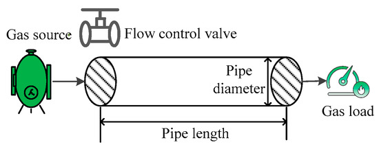
Figure 1.
Gas pipeline schematic diagram.
When considering the dynamic characteristics of gas network pipelines, natural gas has slow transmission speeds and compressibility during pipeline transmission, resulting in unequal gas flow rates at the pipeline inlet and outlet. The portion of natural gas retained in the pipeline is referred to as line pack. Based on this characteristic, the engineer Weymouth derived the relationship between gas flow and pressure using the ideal gas state equation and fluid mechanics principles [25]:
where Pgas,i, Pgas,j, and Ggas,ij represent the inlet node i, outlet node j pressure, and pipeline ij gas flow rate, respectively; Dgas, Lg, fg, and Tg are the inner diameter, length, friction coefficient, and temperature of the pipeline, respectively; and Zg and Rg are the gas constant and compressibility factor, respectively. The parameter sgn indicates the direction, taking values ±1. When sgn(, ) = 1, the airflow direction is from i to j. When sgn(, ) = −1, the airflow direction is from j to i:
To simplify calculations, the quadratic terms of pressure and airflow are piecewise linearized. Introduce auxiliary variables = , = on the right side of Equation (1), replace Ggas,ij|Ggas,ij| on the left side of the equation with a piecewise function, set the positive direction of the airflow as i to j, and the value range of Ggas,ij is [0, ]. The negative direction is j to i, the value range of Ggas,ij is [−, 0], is the upper limit of flow transmission, and the piecewise linearization is shown in Figure 2.
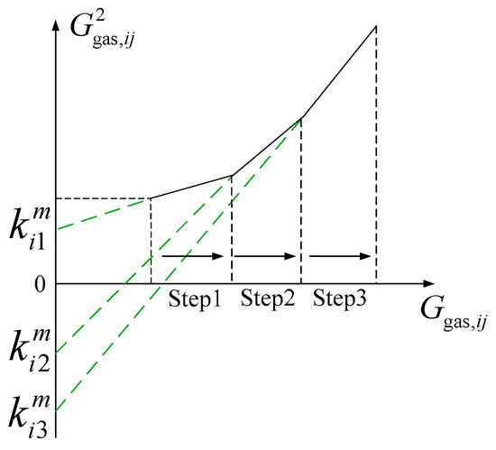
Figure 2.
Piecewise linearization diagram.
Taking the positive direction as an example, by dividing the interval into M equal segments, Equation (1) is transformed as follows:
where is the gas flow rate of segment m at time t; is the slope of segment m; and is a 0–1 variable indicating whether the gas flow rate at time t falls within segment m.
2.2. Dynamic Modeling of Heating Pipes
In heating networks, it is necessary to control the water pressure at both ends of the pipeline to ensure water flow. Therefore, devices such as flow control valves and booster pumps are added. Under the action of booster pumps, heating stations transfer thermal energy to heat loads through supply pipelines. After heat transfer, the water temperature decreases, and the water returns to the heating station through return pipelines, forming a heating cycle, as shown in Figure 3.
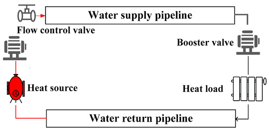
Figure 3.
Schematic diagram of a heating pipeline.
The dynamic characteristics of heating networks mainly manifest in the impact of medium temperature changes, including transmission delay and temperature loss. This paper maintains a constant water flow rate and only considers temperature changes in the heating network and a constant-flow variable-temperature control mode.
The relationship between temperature and thermal power can be expressed as:
where Hheat is the transmission rate of thermal energy required by water flow to provide heat load per unit of time in pipelines; Theat is the temperature that water needs to reach to meet the heat load; cw is the specific heat capacity of water; and μh is the heat dissipation coefficient of the pipeline.
Considering heat transfer delays related to pipeline material, ambient temperature, etc., the supply and return pipeline heat delay times , satisfy [12]:
where ρw is water density; and are the length and cross-sectional area of pipeline b; and and are the flow rates of supply and return pipelines b.
Due to pipeline material and environmental factors, heat loss occurs during heat transfer, causing the water temperature to fall below required standards. Thus, heat loss must be considered. The outlet water temperature of pipelines can be expressed as follows:
where and are the outlet temperatures of supply and return pipelines b; and are the inlet temperatures of supply and return pipelines b; and is the ambient temperature of the pipeline. The heat losses and of the water supply and return pipelines b are:
3. TG-IES Two-Stage Robust Modeling Based on the Dynamic Flow of Gas and Heat Networks
TG and IES achieve energy complementation between different levels through electric power interaction. Meanwhile, CHP (combined heating and power), GB (gas boiler), and EB (electric boiler) energy conversion units make coordinated decisions on the interactive power to achieve the coordinated dispatch of the TG-IES system. The energy flow in the system is shown in Figure 4, including the electric energy interaction between TG-IES and IES-IES, as well as the multi-energy conversion in IES.
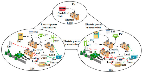
Figure 4.
TG-IES energy flow framework.
3.1. TG-IES System Modeling
3.1.1. Unit Model
Taking IES k at time t as an example, the unit models are as follows:
(1) CHP
where Gk,CHP,t is the natural gas consumed by CHP; Pk,CHPe,t and Hk,CHPh,t are the electricity and heat production power of CHP; and ηCHPe and ηCHPh are the conversion efficiency of CHP electricity and heat.
(2) GB
where Gk,GB,t is the consumption of natural gas in GB; Hk,GBh,t is the GB heat generation power; and ηGBh is the GB heat conversion efficiency.
(3) EB
where Pk,EB,t is the natural gas consumption of EB; Hk,EBh,t is the heat generation power of EB; and ηEBh is the EB heat conversion efficiency.
(4) Energy storage equipment
where Sk,ES,t is the energy storage capacity; Pk,Ech,t and Pk,Edis,t are the charging and discharging power; ηEch and ηEdis are the charging and discharging efficiencies; uk,ess is the charging and discharging state of energy storage, with a variable of 0–1; and is the maximum charging and discharging power.
(5) Carbon trading model
The CO2-emitting units in IES include diesel units, CHP, and GB, and the carbon emission quota is expressed as:
where T is the period set of the scheduling cycle; Pk,dg,t is the output of the diesel unit dg; Ek,C, Ek,dg, Ek,CHP, and Ek,GB are the carbon emission quotas for the system, diesel units, CHP, and GB; and δe and δh are the carbon emission quota coefficients for unit electricity and heat power. The actual carbon emissions of the system are:
where Ek,C,a, Ek,dg,a, Ek,CHP,a, and Ek,GB,a represent the actual carbon emissions of the system, diesel unit, CHP, and GB; and ωe and ωh represent the carbon emission intensity per unit of electrical and thermal power.
Denote Ek,C,a − Ek,C = d, indicating the amount of carbon emissions exceeding the quota. When d < 0, IES provides quantitative subsidies based on the corresponding range of actual carbon emissions. When d > 0, IES purchases carbon quotas beyond the range. The specific model is:
where CCO2 is the cost of carbon trading; u is the reward coefficient; cg is the base price for carbon trading; h is the carbon emission interval value; and ψ is the carbon price growth rate.
3.1.2. Objective Function
This paper takes the scheduling cost CTG-K of the TG-IES system as the target, including the operation cost CTG of TG and the set CK (C1, C2, …, Ck) of IES operation costs.
(1) TG operating cost
where G is the collection of coal-fired units in the transmission network; Pg,t and Cg,t are the output and output cost characteristic functions of unit g at time t, respectively; and ad, bd, and cd are the cost coefficients of thermal power units.
(2) IES operating cost
Taking IES k as an example, its operating costs include power grid cost Ce,k, natural gas network cost Cg,k, and heating network cost Ch,k.
The operating cost of the grid network:
where Gk is the set of diesel units; Cdg,t,k is the cost of the diesel unit dg; PB,t,k and wB are the power output and maintenance coefficients of unit B, including CHP, EB, wind power, and photovoltaic; and CCO2,t,k is the ladder carbon trading cost.
The operating cost of the natural gas network:
where Uk is the collection of natural gas sources, and and cgas,t are the gas flow and gas price of the gas source u, respectively.
The operating cost of the heating network:
where cheat,t is the heating price at time t.
3.1.3. Constraint Condition
Taking IES k at time t as an example, the constraints of TG-IES include TG constraints, IES constraints, and transmission power coupling constraints. The constraints of IES include a power grid, gas network, and heat network [17].
- 1
- TG constraints
TG constraints include power balance, node power balance, line trend, phase angle, unit output, and unit climbing.
where is the power transmitted from TG to IES k; Pd,t is the predicted value of the load; i and j are line nodes; JG is a set of objects connected to node j; fij,t and are the transmission power and upper limit of line ij; Jij, θi,t, θj,t and θrefb,t are the phase angles of the susceptance of line ij, nodes i and j, and relaxed nodes; ug,t is the state variable of unit g; and are the upper and lower limits of the output of unit g; and and are the climbing speeds of unit g up and down the slope.
- 2
- IES Constraints
Power grid constraints include power balance, node power balance, line flow, phase angle, unit output, transmission power, and unit ramp-up.
where Pk,pv,t and Pk,wind,t are the photovoltaic and wind power; Pk,e,t is the predicted value for medium load; is the power of IES m transmitted from IES k; and are the power of TG and IES m received by IES k; a and b are the nodes of the power grid line; J is a set of objects connected to node b in the power grid; fk,ab,t and are the transmission power and upper limit of line ab; Jk,ab, θk,a,t, θk,b,t and θk,refb,t are the phase angles of the susceptance of line ab, nodes a and b, and the relaxation node; and are the upper limits of the output of unit dg and unit B; , , , and are the climbing speeds of unit dg and unit B up and down the slope; and udg,t,k and uB,t,k are the state variables of unit dg and unit B.
The natural gas network constraints include the gas network dynamic model Equation (3), nodal flow balance constraints, gas source output and pipeline flow constraints, and nodal pressure constraints.
where c and d are the nodes of the gas network line; Gk,g,t is the gas load; Gcd,t is the average flow rate of the pipeline cd; pc,t and pd,t are the node c and d air pressure; , are the upper and lower limits of air source output; Gcd,t, , and are the pipeline cd gas flow and upper and lower flow limits; and pc,t, , and are the air pressure and the upper and lower limits of air pressure at node c.
The heat network constraints include the heating network model Equations (5)–(7), the heat power balance constraint, and the supply/return pipeline inlet/outlet temperature constraints.
where Hk,h,t is the heat load; , , and are the water supply pipeline temperature and its upper and lower limits at node o; and , , and are the return pipe temperature and its upper and lower limits at node o.
Transmission power constraint:
where and are the upper limits of variables.
3.2. TG-IES Two-Stage Robust Optimization Model
3.2.1. TG-IES Two-Stage Robust 1st Stage
Without considering uncertain variables, the cost model is:
The compact form of the model is:
where α and β are column vectors of the cost coefficient corresponding to the variable; x and z are the set of state variables; y is the set of decision variables; Ω is the solution of y under certain deterministic (x,z,u′); A, B, C, D, E, and F are the constant coefficient matrix corresponding to the variables; d and h are constant series vectors; and u′ is the predicted value of the uncertain variable, expressed as follows:
where P and P are the initial values of the power transmitted by TG and IES m to IES k at time t, respectively. P′k,pv,t and P′k,wind,t are the predicted photovoltaic and wind power output values at time t, respectively.
Considering the uncertain variables, the uncertainty set U of the box type is established as follows:
where u is the actual output matrix of uncertain variables at time t, and Δu is the maximum fluctuation matrix of uncertain variables at time t.
3.2.2. TG-IES Two-Stage Robust 2nd Stage
The uncertain variable is related to the total output of the unit, and it is necessary to obtain the values of two types of variables: unit start–stop and unit output. Find the optimal solution in the first stage, obtain the start–stop status of each unit, and bring it into the second stage. Find the optimal solution for the worst-case scenario in the second stage under uncertain conditions. Equation (29) can be changed to min-man-min form:
Due to the decrease in the scenic output and the exchange power between IES, the scenic penalty cost and the power generation cost of the units in the park increase, and the increase in the exchange power between TG and IES leads to an increase in the coal consumption cost of the coal-fired units. To simulate the worst scenario, the wind and scenery output and the exchange power between IES are set to the minimum value of the interval, and the exchange power between TG and IES is set to the maximum value of the interval, so Equation (31) can be rewritten as follows:
where γ is the state variable. When the value is 1, the value of the uncertain variable is taken to the interval boundary. Гk,GD, Гk,D, Гk,pv, and Гk,wind are the adjustment parameters of the uncertain variable. The value is an integer from 0 to T, indicating the total number of periods that can reach the boundary of the interval.
Therefore, the two-stage robust optimization problem can be divided into the main problem min and the subproblem max-min, whose coupling and non-convexity make it impossible for the solver to find the two optimal solutions. In this paper, ATC combined with the C&CG algorithm is used to solve the model.
3.3. Model Solving
3.3.1. Two-Stage Robust Model Solution
The C&CG algorithm solves the main problem in the first stage to get the unit start–stop state and combines constraints to solve the man-min problem in the second stage. Through l iterations, the main problem form is obtained as follows:
where σ is the solution of the subproblem; (u′l + γΔul) is the solution of the l times worst scenario; and γΔul is a bilinear term, linearized by the Big-M method:
where γ′ is the auxiliary variable. M1 is a sufficiently large constant number. The subproblem form is:
where xl and zl are the solutions of the l times state variable and the decision variable, respectively.
The max-min is a two-layer optimization problem, which can be transformed into a single-layer optimization problem using KKT conditions. Adding dual constraints and complementary relaxation constraints:
where φ is the dual variable of y.
φTΔu in the complementary relaxation constraint is a bilinear term, and it is linearized by introducing the auxiliary variable v and a sufficiently large constant M2 using the Big-M method:
After transformation, the subproblem form is:
3.3.2. TG-IES Decoupling
Since the transmission power of TG and IES weakens the power supply of TG to the internal load, the coupling constraint needs to be decoupled. By introducing Lagrange multipliers and and penalty factors and combined with two-stage robustness, the model can be expressed as:
where ,,, and are optimized coupled variables; w is the number of iterations; and δμ is the convergence coefficient, with the value of 2~3.
3.3.3. Solution Step
The solving process of the ATC-C&CG algorithm is shown in Figure 5, and the solving steps are as follows:
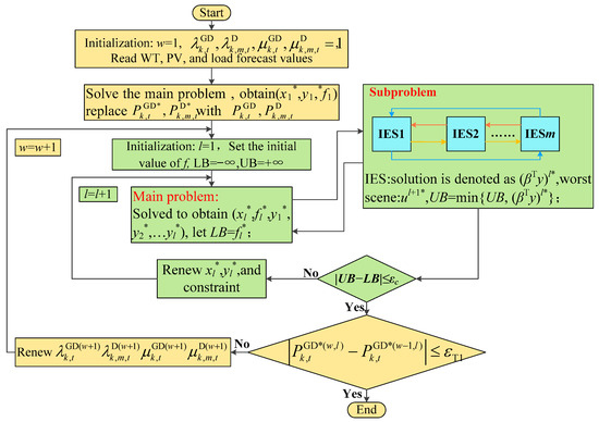
Figure 5.
Solving a flowchart.
- 1
- Initialize the iteration count of the ATC algorithm, w = 1, read the wind and solar prediction values, set the initial values of , , , and to 1, and start the outer loop;
- 2
- Solve Equation (40) to obtain the initial values of the coupling variables and the unit state variables, replace and with and , solve the subproblem of the Equation (40), initialize the iteration number of the C&CG algorithm, l = 1, set the initial lower bound LB = −∞ and initial upper bound UB = +∞ of the objective function, and start the inner loop;
- 3
- During the l iterations, update , , , and alternately, with the optimal solution denoted as (xl*, fl*, y1*, y2*, …yl*). The updated iteration produces fl*, where LB = fl*;
- 4
- Record the solution of the subproblem obtained as (βTyl)*, corresponding to the worst-case scenario ul*, and update the upper bound UB = min{UB, (βTyl)*};
- 5
- Determine the termination condition of the inner loop: Given a sufficiently small convergence threshold εc, if UB − LB ≤ εc, stop the iteration of C&CG, return xl* and yl*, and proceed to step 6. Otherwise, return to step 3;
- 6
- Determine the termination condition of the outer loop: Given sufficiently small convergence thresholds εT1 and εT2. If | − | ≤ εT1, | − | ≤ εT2, stop the iteration of ATC and output the final result. Otherwise, return to step 2 and update , , , and .
4. Results and Discussion
This paper selects the IEEE-39 node power system as the transmission network and the IEEE-39-20-6 node as the IES to construct the TG-IES1-IES2 system. Using MATLAB 2021b software to call the GUROBI solver for solving. The model parameters are shown in reference [25]. The carbon trading model and equipment parameters are shown in Table 1 and Table 2. The topology structure is shown in Figure 6. The predicted values of wind and solar, as known quantities, are shown in Figure 7. The predicted values of loads, as known quantities, are shown in Figure 8.

Table 1.
Carbon trading model parameters.
Table 2.
Equipment parameters.
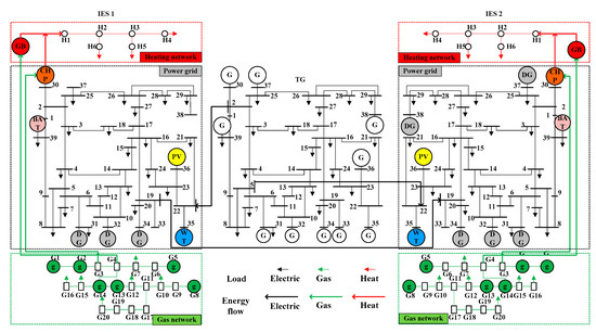
Figure 6.
Topology diagram.
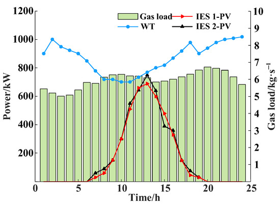
Figure 7.
Wind, solar, and gas load prediction values of the IES system.
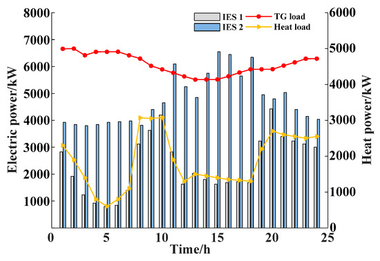
Figure 8.
Forecast values of electrical and thermal loads for the IES system.
4.1. Analysis of Scheduling Results in Different Modes
This chapter sets up four sections to verify the strategy’s effectiveness, as shown in Table 3. The optimization results are presented in Table 4, and the power balance is illustrated in Figure 9.
Table 3.
Different sections.
Table 4.
Comparison of scheduling results under different sections (10 thousand/CNY).
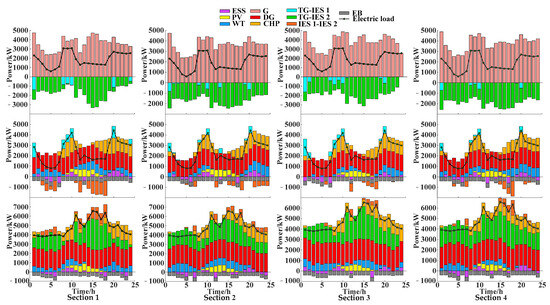
Figure 9.
Different sections of power optimization.
From Table 4, it can be seen that TG, IES1, and IES2 in Section 2 all have reduced costs compared to Section 1. The dynamic model reflects the storage characteristics of gas pipelines and the loss characteristics of thermal pipelines. During periods of high electricity consumption, utilizing stored gas fuel to supply energy to CHP can achieve peak shaving effects and reduce gas purchase costs. At the same time, to meet the energy demand of users under heat loss conditions, the cost of heat loss is reduced by reducing the thermal output of CHP units. At this period, CHP operates according to the working scenario of ordering power by heat, with a decrease in CHP power output and an increase in wind and solar power output, relieving the pressure on the TG power supply, reducing the grid costs of IES1 and IES2, and the total system cost.
Section 3 and Section 4 present the scheduling results for predicted, optimal, and worst-case scenarios, with corresponding uncertainties shown in Figure 9. Compared to Section 3, during the 9:00–19:00 period when electricity consumption is high, the DG and CHP power output of IES1 and IES2 in Section 4 decreases, while the wind and photovoltaic power output increases. When the two-stage robust model is adopted, the scheduling result after adding the dynamic model is better than that of the steady-state model. The optimal period of wind power output and transmission power between subsystems in Section 4 is more than that in Section 3, and the wind power output and carbon yield in each section are also higher than those in other models. In summary, combining dynamic models with two-stage robust strategies can improve the power of new energy and reduce scheduling costs and carbon emissions.
The periods with significant changes in wind power output in Figure 10 are concentrated between 9:00 and 19:00, and between 21:00 and 2:00. In the previous period, the upper limit of wind power was relatively small, and there was a high demand for electricity from users. In the latter period, wind power output is relatively high, resulting in lower electricity demand from users. For the anti-peak characteristic of wind power, energy storage devices can store the remaining electricity generated during low peak periods to meet peak electricity demand. At this moment, the total amount of wind power is relatively low, and there is abundant photovoltaic energy. Wind and photovoltaic power are subject to upper limits. When electricity demand is low, wind power takes the predicted value to obtain the optimal solution in the worst-case scenario.
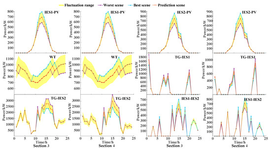
Figure 10.
Uncertain variable power distribution.
From 12:00 to 18:00, IES2 has a high electricity demand, and the output of coal-fired units increases. The TG transmits more power to IES2. The ATC-C&CG algorithm is used to decouple transmission power, improve the distribution autonomy of upper-level TG and lower-level IES, and solve for the optimal solution in the worst-case scenario. At this time, the value of power delivered by the TG to IES1 and IES2 is the lower limit, and the remaining periods are the predicted values. The value of power transmitted from IES1 to IES2 is the upper limit, and the remaining periods are the predicted values. IES1 works with the TG to supply energy to IES2 and relieve the power-supply pressure of the TG.
Figure 11 shows the variation curves of the total cost and carbon emissions concerning the uncertain adjustment parameter Г for both the predicted and actual systems in Mode 4. When the value of Г is less than 7, the total cost and carbon emissions gradually decrease because the number of adverse scenario periods increases, and it is necessary to ensure optimal scheduling in worst-case scenarios. The robust model plays a positive role. As the Г value increases, the duration of adverse scenarios exceeds the actual situation, resulting in a similar scheduling result between predicted and actual scenarios, showing an increasing trend. It is necessary to select an appropriate Г value based on historical data and actual engineering conditions.
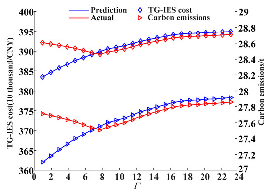
Figure 11.
The impact of Г on system costs and carbon emissions.
This paper compares C&CG with ATC-C&CG to verify the effectiveness of ATC-C&CG in solving distributed robust models. The total cost iteration results are shown in Figure 12. After joining ATC, the transmission power is decoupled through Lagrange multipliers and penalty factors to achieve parallel computing of TG and IES. The costs of TG, IES1, and IES2 are balanced, and the cost iteration curve is shown in Figure 13. In the iterative calculation of ATC, C&CG jumps out of the loop after only one iteration, and the target value converges after five iterations. Using only C&CG to solve the model requires seven iterations, a longer computation time, and an additional cost of CNY 0.3365 thousand. Based on the above analysis, ATC-C&CG has improved the efficiency and accuracy of solving the model.
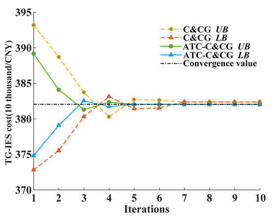
Figure 12.
Algorithm convergence curves.
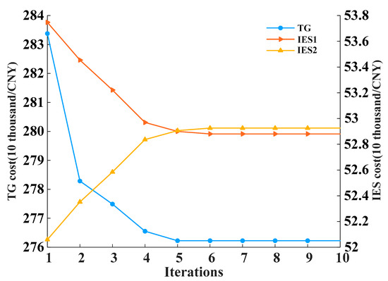
Figure 13.
Iteration curves for each system cost.
4.2. Dynamic Characteristic Effect Analysis
The total amount of gas purchased by IES under different sections is shown in Figure 14. Compared with the comparison Section 1, Section 2, and Section 3, the gas source output of Section 4 decreased by 0.3046 km3, 0.0077 km3, and 0.1528 km3, respectively. Compared with Section 1 and Section 3, Section 2 and Section 4 have reduced gas purchases. Due to the lower energy demand from 3:00 to 5:00, the CHP output of IES1 and IES2 is 0. By utilizing the characteristics of pipeline storage, the remaining natural gas produced by the gas source is stored and used as fuel for CHP and GB from 7:00 to ~10:00 and from 17:00 to ~24:00, reducing the amount of gas purchased and thus reducing the cost of gas purchase, as shown in Figure 15. Compared to Section 3, Section 4 has reduced CHP output. The two-stage robust model can expand the solution space and solve for the optimal gas source output in the worst-case scenario, further reducing the gas purchase volume in Section 4.
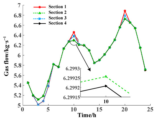
Figure 14.
Total output of different modes of gas supply.
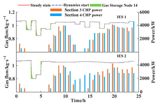
Figure 15.
Changes in gas source node flow and CHP output.
The thermal energy optimization of Section 3 and Section 4 is shown in Figure 16 and Figure 17. Due to the lack of consideration for the dynamic characteristics of the heating network in Section 3, the total heat output of the units in each period is equal to the heat load. During the 12:00~19:00 period, Section 4 stores the remaining thermal energy produced by CHP, GB, and EB. Release from 0:00 to 11:00 and 20:00 to 0:00 to supplement the portion of heat energy that is less than the heat load of the unit, thereby reducing pipeline heat loss and heating costs. The average temperature changes with the storage and release of heat energy. Comparing the variation curves of heat load and temperature, the thermal delay characteristic results in partial temperature delay.
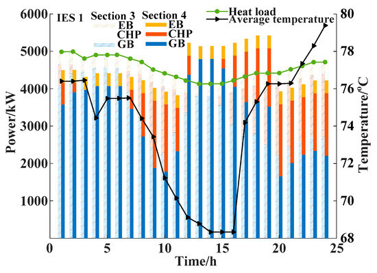
Figure 16.
Thermal optimization and temperature change of IES1.
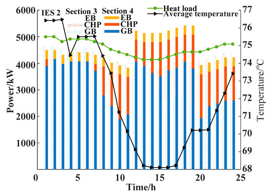
Figure 17.
Thermal optimization and temperature change of IES2.
5. Conclusions
This paper presents a two-stage robust scheduling model for TG-IES, based on the gas thermal dynamic characteristics. The model is solved using ACT and C&CG algorithms, and the following conclusions are obtained:
- 1
- The total scheduling cost of the optimal Section 4 is reduced by 0.49%, 0.24%, and 0.15% compared to Section 1, Section 2, and Section 3, respectively, reflecting the dynamic characteristics of gas and heat and the two-stage robust model’s significant support for uncertainty variable solving and economic operation of the transmission grid multi-park collaborative system.
- 2
- After adopting a two-stage robust model, the total cost of optimal Section 3 and Section 4 is lower than that of Section 1 and Section 2, reflecting the flexibility of two-stage robust models in solving uncertainty problems. On this basis, considering the dynamic characteristics of gas and heat, utilizing the gas “pipe storage” characteristic to improve the system’s multi-energy complementarity, the scheduling cost of Section 4 is further reduced.
This article focuses on the power exchange scheduling of multi-park systems and has not yet considered the interaction of gas and heat energy between parks. In subsequent research, the impact of gas thermal dynamic characteristics on the interaction system of gas and thermal energy flow in multiple parks can be analyzed, as well as the optimization of the interaction system’s operation.
Author Contributions
Conceptualization, J.W., T.Z., W.L. and M.C.; Methodology, J.W., T.Z. and M.C.; Software, J.W.; Validation, J.W. and W.L.; Formal analysis, J.W., T.Z., W.L. and M.C. All authors have read and agreed to the published version of the manuscript.
Funding
This research received no external funding.
Data Availability Statement
The original contributions presented in this study are included in the article. Further inquiries can be directed to the corresponding author(s).
Conflicts of Interest
The authors declare that they have no known competing financial interests or personal relationships that could have appeared to influence the work reported in this paper.
Abbreviations
| IES | integrated energy system |
| TG | transmission grid |
| ATC | analytical target cascading |
| C&CG | column and constraint generation |
| CHP | combined heating and power |
| GB | gas boiler |
| EB | electric boiler |
References
- Liu, L.; Hu, X.; Chen, J.; Wu, R.; Chen, F. Embedded scenario clustering for wind and photovoltaic power, and load based on multi-head self-attention. Prot. Control Mod. Power Syst. 2024, 9, 122–132. [Google Scholar] [CrossRef]
- Zhang, G.; Liu, J.; Xie, T.; Zhang, K. Low-carbon optimization operation of rural energy system considering high-level water tower and diverse load characteristics. Processes 2025, 13, 1366. [Google Scholar] [CrossRef]
- Jiang, T.; Wu, C.; Li, X.; Zhang, R.; Fu, L. Clearing mechanism of energy-flexibility markets with transmission and distribution coordination considering charging and discharging of electric vehicles. Autom. Electr. Power Syst. 2024, 48, 210–224. [Google Scholar]
- Zhang, Y.; Su, Y. Research on influencing factors of rural residents living energy structure transformation towards sustainable development. Value Eng. 2020, 39, 287–292. [Google Scholar]
- Cai, J.; Wang, Y.; Xu, X.; Xiong, W.; Guo, T.; Miao, S.; Miu, S. Joint optimization model of power grid unit commitment and technical transformation plan considering transmission and distribution coordination. Electr. Power Autom. Equip. 2023, 43, 174–183. [Google Scholar]
- Wang, M.; Zhao, H.; Liu, C.; Ma, H. Dynamic energy flow tracking and carbon entropy analysis of integrated energy system based on superposition principle. Autom. Electr. Power Syst. 2024, 48, 10–20. [Google Scholar]
- Li, Z.; Xu, Y.; Wang, P.; Xiao, G. Coordinated preparation and recovery of a post-disaster multi-energy distribution system considering thermal inertia and diverse uncertainties. Appl. Energy 2023, 336, 120736. [Google Scholar] [CrossRef]
- Dong, S.; Wang, C.; Xu, S.; Zhang, L.; Zha, H. Day-ahead optimal scheduling of electricity-gas-heat integrated energy system considering dynamic characteristics of networks. Autom. Electr. Power Syst. 2018, 42, 12–19. [Google Scholar]
- Chen, X.; Wang, C.; Wu, Q.; Dong, X.; Liang, J. Optimal operation of integrated energy system considering dynamic heat-gas characteristics and uncertain wind power. Energy 2020, 198, 117270. [Google Scholar] [CrossRef]
- Qin, X.; Sun, H.; Shen, X. A generalized quasi-dynamic model for electric-heat coupling integrated energy system with distributed energy resources. Appl. Energy 2019, 251, 113270. [Google Scholar] [CrossRef]
- Lin, Z.; Zhu, X.; Wang, S.; Gao, L.; Yu, Y.; Wang, S. Optimal scheduling of electric-thermal integrated energy system considering dynamic characteristics of heating network and carbon trading. Proc. CSU-EPSA 2022, 34, 64–70. [Google Scholar]
- Zhang, H.; Cheng, Z.; Jia, R.; Zhou, C.; Li, M. Economic optimization of electric-gas integrated energy system considering dynamic characteristics of natural gas. Power Syst. Technol. 2021, 45, 1304–1311. [Google Scholar]
- Lin, Y.; Shao, Z.; Chen, F.; Chen, Y.; Deng, H. Distributed low-carbon economic scheduling of integrated electricity and gas system based on gas network division. Power Syst. Technol. 2023, 47, 2639–2645. [Google Scholar]
- Mei, J.; Wei, Z.; Zhang, Y.; Ma, Z.; Sun, G.; Zang, H. Dynamic optimal dispatch with multiple time scale in integrated power and gas energy systems. Autom. Electr. Power Syst. 2018, 42, 36–42. [Google Scholar]
- Yang, J.; Ning, Z.; Kang, C.; Xia, Q. Effect of natural gas flow dynamics in robust generation scheduling under wind uncertainty. IEEE Trans. Power Syst. 2017, 33, 2087–2097. [Google Scholar] [CrossRef]
- Wang, W.; Wang, X.; Xu, Y.; Wang, Y.; Liu, J.; Du, Y. A synthetic optimal decision-making method for parallel restoration sectionalizing and generator start-up sequence of power grids considering transmission and distribution system coordination. Proc. CSEE 2024, 44, 859–872. [Google Scholar]
- Zhang, X.; Zhang, Y.; Ji, X.; Han, X.; Yang, M.; Xu, B. Synergetic optimized scheduling of transmission and distribution network with electricity-gas-heat integrated energy system. Power Syst. Technol. 2022, 46, 4256–4270. [Google Scholar]
- Zhang, Y.; Zhang, X.; Ji, X.; Han, X.; Wang, C.; Yu, Y. Synergetic unit commitment of transmission and distribution network considering dynamic characteristics of electricity-gas-heat integrated energy system. Proc. CSEE 2022, 42, 8576–8592. [Google Scholar]
- Liu, Y.; Guo, L.; Wang, C. Economic dispatch of microgrid based on two stage robust optimization. Proc. CSEE 2018, 38, 4013–4022. [Google Scholar]
- Li, M.; Mei, W.; Zhang, L.; Bai, B.; Zhao, C.; Cai, L. Research on multi-energy microgrid scheduling optimization model based on renewable energy uncertainty. Power Syst. Technol. 2019, 43, 1260–1270. [Google Scholar]
- Cao, M.; Xie, C.; Li, F.; Yi, C.; Zhang, G.; Gao, Y. Co-optimized operation of multi-integrated energy microgrids-shared energy storage. Power Syst. Technol. 2024, 48, 4493–4502. [Google Scholar]
- Zhou, T.; Xue, Y.; Ji, J.; Han, Y.; Bao, W.; Li, F.; Du, E.; Zhang, N. A two-stage robust optimization method for electricity-cooling-heat integrated energy system considering uncertainty of indirect carbon emissions of electricity. Power Syst. Technol. 2024, 48, 50–63. [Google Scholar]
- Yi, Y.; Xu, J.; Zhang, W.; Li, Y. Multi-microgrid cooperative game considering two-stage robust optimal configuration. Autom. Electr. Power Syst. 2023, 47, 149–156. [Google Scholar]
- Xu, Y.; Zhang, S.; Zhang, T.; Mi, L. Cooperative optimal operation of multi-microgrids based on hybrid two-staged robustness. Power Syst. Technol. 2024, 48, 247–267. [Google Scholar]
- Deng, H. Evaluating Nodal Energy Price of Carbon Emission-Embedded Electricity-Gas-Heat Integrated Energy System. Master’s Thesis, Northeast Electric Power University, Jilin, China, 2019. [Google Scholar]
Disclaimer/Publisher’s Note: The statements, opinions and data contained in all publications are solely those of the individual author(s) and contributor(s) and not of MDPI and/or the editor(s). MDPI and/or the editor(s) disclaim responsibility for any injury to people or property resulting from any ideas, methods, instructions or products referred to in the content. |
© 2025 by the authors. Licensee MDPI, Basel, Switzerland. This article is an open access article distributed under the terms and conditions of the Creative Commons Attribution (CC BY) license (https://creativecommons.org/licenses/by/4.0/).