A Day-Ahead Optimization of a Distribution Network Based on the Aggregation of Distributed PV and ES Units

Abstract

The increasing penetration of distributed photovoltaic (PV) and energy storage (ES) systems in power grids, while advancing the transition to clean energy and enhancing grid flexibility, poses resource dispersion, uncertainty, and scheduling challenges. Consequently, it becomes crucial to manage and optimize these resources. In this paper, we innovatively propose a distribution network day-ahead optimal scheduling model that takes into account distributed resource aggregation and uncertainty. Firstly, distributed PV aggregation (PVA) is performed using the Minkowski summation method, and distributed ES aggregation (ESA) is performed using the polytope inner approximation method. Then, in order to deal with the uncertainty, the supply–demand balance of flexibility is modeled using kernel density estimation (KDE). Finally, the aggregation model and the flexibility supply–demand balance model are incorporated into the distribution network day-ahead optimization. The simulation study of the IEEE 69-node distribution system shows that the aggregate feasible region (AFR) is improved by about 90% and the active flexibility is improved by about 10% compared to box inner approximate aggregation methods, demonstrating their effectiveness in managing operational uncertainties and optimizing the utilization of distributed energy resources in day-ahead scheduling.

1. Introduction

Against the backdrop of energy transition and policy support, rooftop PV and household energy storage systems are developing rapidly due to technological advances and cost reductions, becoming important forms of clean energy utilization. Therefore, the continuous integration of a wide range of distributed renewable energy sources into the grid has significantly increased the complexity of distribution network scheduling [1]. It mainly stems from the spatial–temporal dispersion of resources, random power fluctuations, and multidimensional operation constraints. Traditional decentralized management makes it hard to coordinate the heterogeneous features of distributed PV and ES, which can easily lead to reverse current and the waste of regulation potential. Distributed resource aggregation integrates distributed units into aggregates through clustering management and control and uses aggregation methods to compress uncertainty intervals and improve flexible regulation capability.

Aggregators must understand the flexibility of PV units and ES units, specifically by constructing AFR to determine acceptable power profiles [2,3]. In practice, the precise AFR corresponds to the Minkowski sum of the feasible regions of all PV and ES units. Direct Minkowski summation for PV systems is both accurate and computationally efficient. However, performing Minkowski sum operations on polytopes under H-representation is generally NP-hard [4]. The set of admissible power profiles for an ES unit is typically represented as the intersection of a collection of half-spaces, a concept known as the H-representation of a polytope [5]. As a result, some researchers have focused on deriving an approximate AFR that maintains acceptable computational complexity. These approximate methods can be broadly categorized into two types: outer approximation and inner approximation. Outer approximation methods typically obtain the approximate AFR through linear summation [6]. The virtual battery model, as presented in [7,8], is used to describe the flexibility of individual electric vehicles, with their energy and power bounds being summed to derive the aggregate bounds. To enhance the accuracy, Barot and Taylor [9] propose a general outer approximation method for the Minkowski sum of polytopes, while an equivalent time-variant storage model is developed in [10] by incorporating time-dependent constraints for aggregation. In general, these methods are straightforward and computationally efficient. However, they may lead to the inclusion of infeasible regions, which could result in violations of the original energy storage constraints during the disaggregation process. To ascertain the viability of the disaggregation process, several inner approximation methods have been proposed. References [11,12] formulate optimization problems to maximize the difference between the upper and lower bounds, a technique commonly referred to as the box-based method. However, this method is typically conservative and may exclude a significant portion of the AFR. Consequently, several geometric approaches have been developed to better capture the feasible regions of energy storage, including zonotope-based [13], ellipsoid-based [14], and polytope-based [15,16] methods. Among these, the polytope-based inner approximation method offers higher accuracy for linear and convex models compared to other methods [17]. Therefore, further research is needed to improve aggregation accuracy while maintaining computational efficiency and to explore how the AFR can be effectively utilized for optimal scheduling following aggregation.

At the same time, the expansion of renewable energy sources has led to a rapid increase in the demand for system flexibility. Assuming that fossil fuel generators provide all the flexibility, in this case, this operational paradigm not only compromises the environmental benefits inherent in renewable energy systems but also escalates the marginal costs of power system operations while constraining the potential for further renewable capacity integration [18]. As a large number of ES units are integrated into the distribution network, they present significant flexibility potential that can improve both the economical and reliable operation of the system by providing a variety of ancillary services, such as reserve capacity [19,20] and peaking services [21]. For the distribution network, the system flexibility refers to the ability to deploy its resources to respond to changes in the net load [22]. In addition, the application of advanced ICT promotes the evolution from a traditional power grid to a Smart Grid [23], which provides possibilities for new technologies. At present, the existing research on distributed flexibility coordination can be summarized as the following six methods according to flexibility supply [24,25,26]: demand response-based approach, dispatchable distributed generators-based approach (e.g., microturbines), ES-based approach, grid interconnection-based approach, renewable energy curtailment-based approach, and load shedding-based approach. Note that the above first four approaches can be regarded as proactive methods, while the last two are passive ones. Therefore, it is an important challenge to quantify the flexibility supply–demand balance of the distribution system.

To address the limitations of these existing methods, this paper proposes a fast aggregation technique based on Minkowski summation and polytope inner approximation, which allows for the rapid determination of the feasible regions for both active and reactive power. Additionally, a distribution network day-ahead optimization strategy that accounts for aggregators and uncertainty is proposed. The main contributions of this paper are as follows:

• A PV and ES aggregation method is proposed, which determines the AFR for active and reactive power through Minkowski summation and polytope inner approximation, providing dispatchable capabilities for subsequent optimal scheduling.
• A conservative representation of probability density confidence intervals is developed for new energy and load uncertainties. The flexibility supply and demand balance is derived through the KDE method. Confidence levels are incorporated to transform the uncertainty of PV systems and load into a deterministic flexibility balance problem.
• A day-ahead optimal scheduling method based on the proposed PV and ES aggregation model and flexibility supply and demand balance is proposed, which helps achieve the aggregation of distributed resources and the overall strategy of distribution network scheduling.

The rest of the paper is organized as follows. Section 2 constructs the distributed PV and ES aggregation model. Section 3 details the distribution network flexibility balancing. Section 4 describes the day-ahead distribution network optimization considering aggregation and uncertainty. Numerical case studies demonstrate the effectiveness of the proposed model in Section 5. Finally, Section 6 concludes the paper.

2. AFR for Distributed PV and ES

The development and utilization of large-scale distributed resources make them small, numerous, and dispersed and, thus, poorly scheduled by traditional methods. Therefore, in the context of PV and ES systems, the concept of aggregation is introduced to effectively aggregate these distributed resources and participate in network optimization and scheduling as a whole.

2.1. Aggregation of Distributed PV Units

For PV units, the feasible regions of active and reactive power form a convex set in the two-dimensional plane so that active and reactive power aggregation can be performed directly by the Minkowski summation method.

Minkowski summation is the sum of the point sets of two Euclidean spaces, also known as the expansion set of these two spaces. Given two point sets $Z^{\mathrm{a}}$ and $Z^{\mathrm{b}}$, point set $Z^{\mathrm{c}}$ is defined as the Minkowski sum of the two points. This addition is performed by adding the corresponding x-coordinates and the corresponding y-coordinates, and the point set $Z^{\mathrm{c}}$ is the Minkowski summation of $Z^{\mathrm{a}}$ and $Z^{\mathrm{b}}$. Thus, the basic form of Minkowski summation is:

$$Z^{\mathrm{c}}=Z^{\mathrm{a}}\oplus Z^{\mathrm{b}}=\{a+b| a\in Z^{\mathrm{a}},b\in Z^{\mathrm{b}}\}$$

(1)

The PV unit feasible region can be represented in a vector form:

$$Z_n^{\mathrm{PV}}=(P_n^{\mathrm{PV}},Q_n^{\mathrm{PV}})$$

(2)

where $Z_n^{\mathrm{PV}}$ is the feasible region of the PV unit $n$, $P_n^{\mathrm{PV}}$ is the feasible active power of the PV unit $n$, and $Q_n^{\mathrm{PV}}$ is the feasible reactive power of the PV unit $n$.

Therefore, the feasible region of the PVA is:

$$Z_m^{\mathrm{PVA}}=Z_1^{\mathrm{PV}}\oplus Z_2^{\mathrm{PV}}\dots \dots \oplus Z_n^{\mathrm{PV}}$$

(3)

where $Z_m^{\mathrm{PVA}}$ is the feasible region of the PVA $m$.

Further derivation of the AFR is conducted after the aggregation of PV. The feasible regions of PV unit 1 and PV unit 2 are shown below, represented in the vector form and satisfying the active power and reactive power constraints:

$$\left\{\begin{array}{l}{Z}_1^{\mathrm{PV}}=(P_1^{\mathrm{PV}},Q_1^{\mathrm{PV}})\\ Z_2^{\mathrm{PV}}=(P_2^{\mathrm{PV}},Q_2^{\mathrm{PV}})\end{array}\right.$$

(4)

$$\left\{\begin{array}{l}{(P_1^{\mathrm{PV}})}^2+{(Q_1^{\mathrm{PV}})}^2\le {(S_1^{\mathrm{PV}})}^2\\ {(P_2^{\mathrm{PV}})}^2+{(Q_2^{\mathrm{PV}})}^2\le {(S_2^{\mathrm{PV}})}^2\end{array}\right.$$

(5)

Theorem 1.

According to Minkowski inequality [27]:

$$‖Z_1^{\mathrm{PV}}+Z_2^{\mathrm{PV}}‖\le ‖Z_1^{\mathrm{PV}}‖+‖Z_2^{\mathrm{PV}}‖$$

(6)

where $‖Z_1^{\mathrm{PV}}‖$ is the vector norm of PV 1, $‖Z_2^{\mathrm{PV}}‖$ is the vector norm of PV 2, and $‖Z_1^{\mathrm{PV}}+Z_2^{\mathrm{PV}}‖$ is the vector norm of PVA.

Proof of Theorem 1.

Further obtained from Equation (6):

$$\sqrt{(P_1^{\mathrm{PV}}+P_2^{\mathrm{PV}}{)}^2+(Q_1^{\mathrm{PV}}+Q_2^{\mathrm{PV}}{)}^2}\le \sqrt{(P_1^{\mathrm{PV}}+Q_1^{\mathrm{PV}}{)}^2}+\sqrt{(P_2^{\mathrm{PV}}+Q_2^{\mathrm{PV}}{)}^2}$$

(7)

Combining with Equation (5) to obtain:

$$\sqrt{(P_1^{\mathrm{PV}}+P_2^{\mathrm{PV}}{)}^2+(Q_1^{\mathrm{PV}}+Q_2^{\mathrm{PV}}{)}^2}\le S_1^{\mathrm{PV}}+S_2^{\mathrm{PV}}$$

(8)

The final aggregation constraint is obtained:

$$\left\{\begin{array}{l}{P}_m^{\mathrm{PVA}}=P_1^{\mathrm{PV}}+P_2^{\mathrm{PV}}\\ Q_m^{\mathrm{PVA}}=Q_1^{\mathrm{PV}}+Q_2^{\mathrm{PV}}\\ (P_m^{\mathrm{PVA}}{)}^2+(Q_m^{\mathrm{PVA}}{)}^2\le (S_m^{\mathrm{PVA}}{)}^2\end{array}\right.$$

(9)

where $P_m^{\mathrm{PVA}}$ is the active power of PVA $m$, and $Q_m^{\mathrm{PVA}}$ is the reactive power of PVA $m$.

Therefore, for PVA active and apparent power can be directly summed to obtain the feasible region according to the constraints of Equation (9).

Based on the PV prediction curve, the actual PV power output at each time is derived:

$$P_{m,t}^{\mathrm{PVA}}={\partial }_t{P}_m^{\mathrm{PVA}}$$

(10)

where ${\partial }_t$ is the PV prediction coefficient at time $t$, and $P_m^{\mathrm{PVA}}$ is the active power of PVA $m$. □

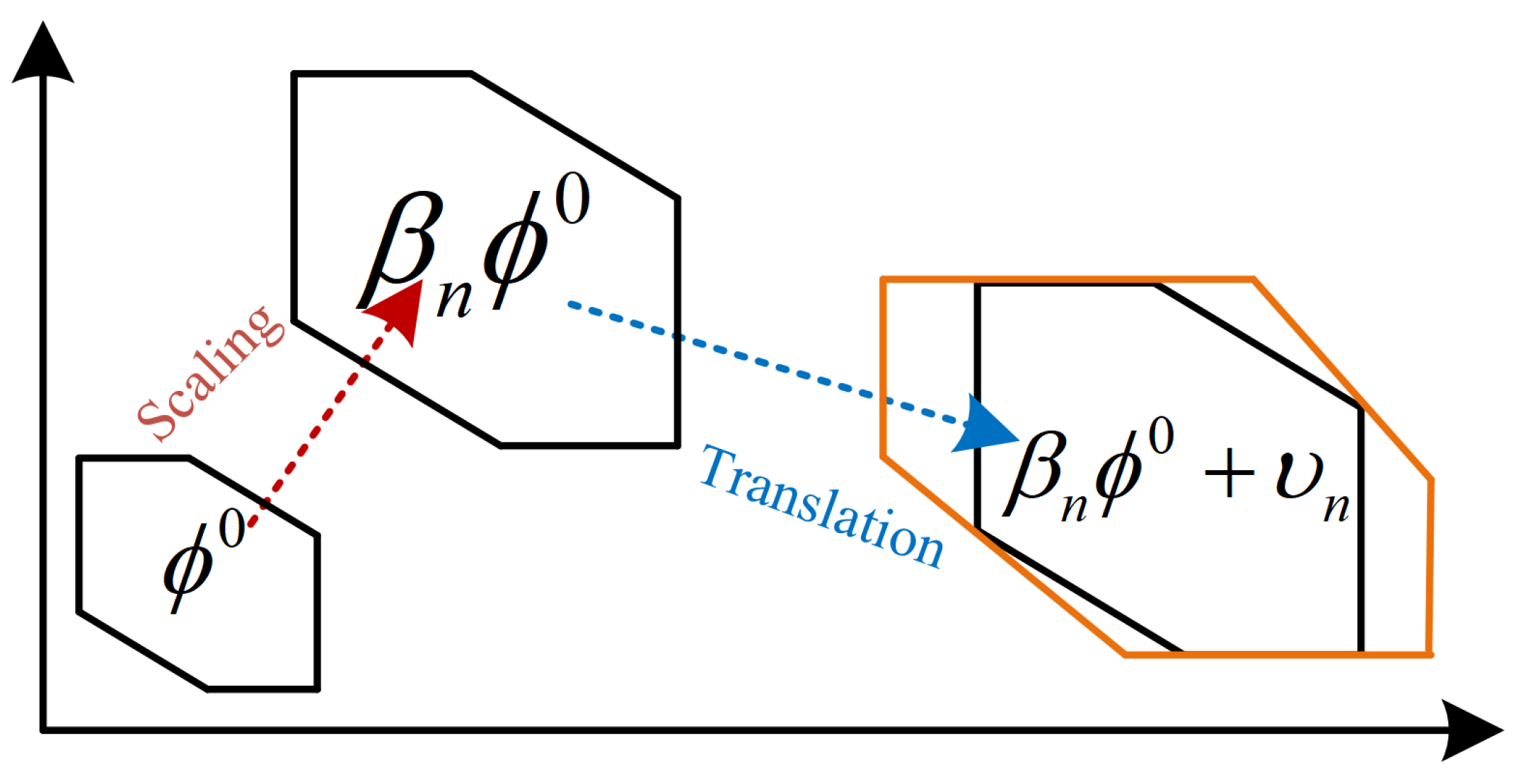
2.2. Aggregation of Distributed ES Units

The mathematical model for charging and discharging an ES unit is given by the following:

$$\left\{\begin{array}{l}0\le P_{n,t}^{\mathrm{ch}}\le P_n^{\mathrm{ch},\max }\\ 0\le P_{n,t}^{\mathrm{dch}}\le P_n^{\mathrm{dch},\max }\\ E_{n,t+1}=E_{n,t}+({\eta }_n^{\mathrm{ch}}{P}_{n,t}^{\mathrm{ch}}-{\displaystyle \frac{P_{n,t}^{\mathrm{dch}}}{{\eta }_n^{\mathrm{dch}}}})\Delta t\\ 0\le E_{n,t}\le E_n^{\max }\end{array}\right.$$

(11)

where $P_{n,t}^{\mathrm{ch}}$ and $P_{n,t}^{\mathrm{dch}}$ are the charging power and discharging power of the ES unit $n$ at time $t$, respectively; $E_{n,t}$ is the battery capacity of the ES unit $n$ at time $t$; ${\eta }_n^{\mathrm{ch}}$ and ${\eta }_n^{\mathrm{dch}}$ are the charging and discharging power efficiencies of the ES unit $n$, respectively.

The mathematical model of ES can be represented in a polytope form, as shown in Equation (12).

$${\mathsf{\Omega }}_n=\left\{P_n\in {ℝ}^{2r}|M_n{P}_n<N_n\right\}$$

(12)

where $P_n={[P_n^{\mathrm{ch}},P_n^{\mathrm{dch}}]}^T$, $P_n^{\mathrm{ch}}={[P_{n,t}^{\mathrm{ch}}]}_{1\times r}^T$, $P_n^{\mathrm{dch}}={[P_{n,t}^{\mathrm{dch}}]}_{1\times r}^T$.

$M_n$ and $N_n$ are expressed as, respectively:

$$M_n=\left[\begin{array}{cc}{I}_r& 0\\ 0& I_r\\ -I_r& 0\\ 0& -I_r\\ B_n^{\mathrm{ch}}& -B_n^{\mathrm{dch}}\\ -B_n^{\mathrm{ch}}& B_n^{\mathrm{dch}}\end{array}\right]$$

(13)

where $I_r$ is an r-dimensional identity matrix, and $B_n^{\mathrm{ch}}$ and $B_n^{\mathrm{dch}}$ are r-dimensional lower triangular matrices:

$$\left\{\begin{array}{l}{B}_n^{\mathrm{ch}}=diag{(\Delta t{\eta }_n^{\mathrm{ch}})}_{r\times r}\\ B_n^{\mathrm{dch}}=diag{(\Delta t/{\eta }_n^{\mathrm{dch}})}_{r\times r}\end{array}\right.$$

(14)

$$N_n=\left[\begin{array}{l}{P}_n^{\mathrm{ch},\max }\\ P_n^{\mathrm{dch},\max }\\ 0\\ 0\\ E_n^{\max }-E_n^0\\ E_n^0-E_n^{\min }\end{array}\right]$$

(15)

where $P_n^{\mathrm{ch},\max }$, $P_n^{\mathrm{dch},\max }$, $E_n^{\max }$, $E_n^{\min }$, $E_n^0$ are r-dimensional column vectors. $P_n^{\mathrm{ch},\max }={[P_n^{\mathrm{ch},\max }]}_{r\times 1}$, $P_n^{\mathrm{dch},\max }={[P_n^{\mathrm{dch},\max }]}_{r\times 1}$, $E_n^{\max }={[E_n^{\max }]}_{r\times 1}$, $E_n^{\min }={[E_n^{\min }]}_{r\times 1}$, $E_n^0={[E_n^0]}_{r\times 1}$.

To ensure the feasibility of the aggregation, this paper uses the polytope inner approximation method. This method ensures that the dispatch signals from the higher-level grid are feasible and can be efficiently disaggregated for implementation.

Theorem 2.

Firstly, the basis aggregate matrix is constructed according to ${\varphi }_k^0(M_k^0,N_k^0)$ , $M_k^0$ and $N_k^0$ are the average of all the ES parameters. Then, a series of same-type ${\varphi }_k^0$ to each ES ${\varphi }_n$ is generated by scaling and translating the basis matrices so that $M$ of same-type polygons is conveniently computed as follows:

$$\widetilde{{\varphi }_n}={\beta }_n{\varphi }_k^0+{\upsilon }_n=\left\{P_n\in {ℝ}^{2r}|M_k^0(P_n-\right.{\upsilon }_n)\le \left.{\beta }_n{N}_k^0\right\}$$

(16)

$$({\beta }_1{\varphi }_k^0+{\upsilon }_1)\oplus ({\beta }_2{\varphi }_k^0+{\upsilon }_2)=({\beta }_1+{\beta }_2){\varphi }_k^0+({\upsilon }_1+{\upsilon }_2)$$

(17)

where $\widetilde{{\varphi }_n}$ is ${\varphi }_n$’s the inner approximate feasible region, ${\beta }_n$ and ${\upsilon }_n$ are the scaling and translating factors, respectively.

Proof of Theorem 2.

Given a convex set ${\varphi }_k^0=\left\{\left.P_n|M_k^0{P}_n\le N_k^0\right\}\right.$, after scaling and translating, the same type ${\varphi }_k^0$ can be expressed as

$${\beta }_n{\varphi }_k^0+{\upsilon }_n:=\left\{U_n|U_n={\beta }_n{P}_n+{\upsilon }_n,\forall P_n\in {\varphi }_k^0\right\}$$

(18)

Equation (18) is equivalent:

$${\beta }_n{\varphi }_k^0+{\upsilon }_n:=\left\{U_n|U_n={\beta }_n{P}_n+{\upsilon }_n,M_k^0{P}_n\le N_k^0\right\}$$

(19)

$P_n$ can be expressed as:

$$P_n={\displaystyle \frac{U_n-{\upsilon }_n}{{\beta }_n}}$$

(20)

Equations (18) and (19) can be expressed as:

$${\beta }_n{\varphi }_k^0+{\upsilon }_n:=\left\{U_n|M_k^0(U_n-{\upsilon }_n)\le {\beta }_n{N}_k^0\right\}$$

(21)

Replacing $U_n$ with $P_n$ yields Equation (16).

As shown in Figure 1, ${\beta }_n$ is used to zoom in on the prototype and determine the size of the feasible region and ${\upsilon }_n$ is used to translate the prototype and determine the location of the feasible region. Therefore, to obtain the maximum inner approximation region, the following problem is established:

$$\begin{array}{l}\underset{{\beta }_n,{\upsilon }_n}{\max }{\beta }_n\\ \mathrm{s}.\mathrm{t}. {\beta }_n{\varphi }_k^0+{\upsilon }_n\subseteq {\varphi }_n,{\beta }_n\ge 0\end{array}$$

(22)

According to Farkas’ derivation, the above-set inclusion problem is equivalent to the following equation and inequality problem, the proof of which can be found in Appendix A [15]:

$$\begin{array}{l}\underset{{\beta }_n,{\upsilon }_n,G}{\max }{\beta }_n\\ \mathrm{s}.\mathrm{t}. G{M}_k^0=M_n,G\ge 0\\ {\beta }_{n}G{N}_k^0+M_n{\upsilon }_n\le N_n,{\beta }_n\ge 0\end{array}$$

(23)

where $G$ is the assisted matrix.

Due to its variable-solving problem, introducing the assistant parameters and letting $b_n=1/{\beta }_n,r_n=-{\upsilon }_n/{\beta }_n$, the following equation can be further obtained:

$$\begin{array}{l}\underset{b_n,r_n,G}{\min }{b}_n\\ \mathrm{s}.\mathrm{t}. G{M}_k^0=M_n,G\ge 0\\ G{N}_k^0\le b_n{N}_n+M_n{r}_n,b_n\ge 0\end{array}$$

(24)

The active and reactive power mathematical formulas are then used to summarize and solve for the feasible region of reactive power, which ultimately leads to the ES active and reactive power feasible region and the upper and lower battery capacity limits.

$$(P_{m,t}^{\mathrm{ESA}}{)}^2+(Q_{m,t}^{\mathrm{ESA}}{)}^2\le (S_m^{\mathrm{ESA}}{)}^2$$

(25)

where $P_{m,t}^{\mathrm{ESA}}$ is the active power of the ES aggregator (ESA) $m$ at time $t$, $Q_{m,t}^{\mathrm{ESA}}$ is the reactive power of the ESA $m$ at time $t$, and $S_m^{\mathrm{ESA}}$ is the apparent power of the ESA $m$. □

3. Flexible Supply and Demand Balance

The integration of a large number of new energy sources into the distribution network increases the volatility, uncertainty, and a lack of flexibility. Therefore, the flexibility supply–demand balance model is constructed to convert the uncertainty problem into a deterministic problem and incorporate it into the optimal scheduling of the distribution network.

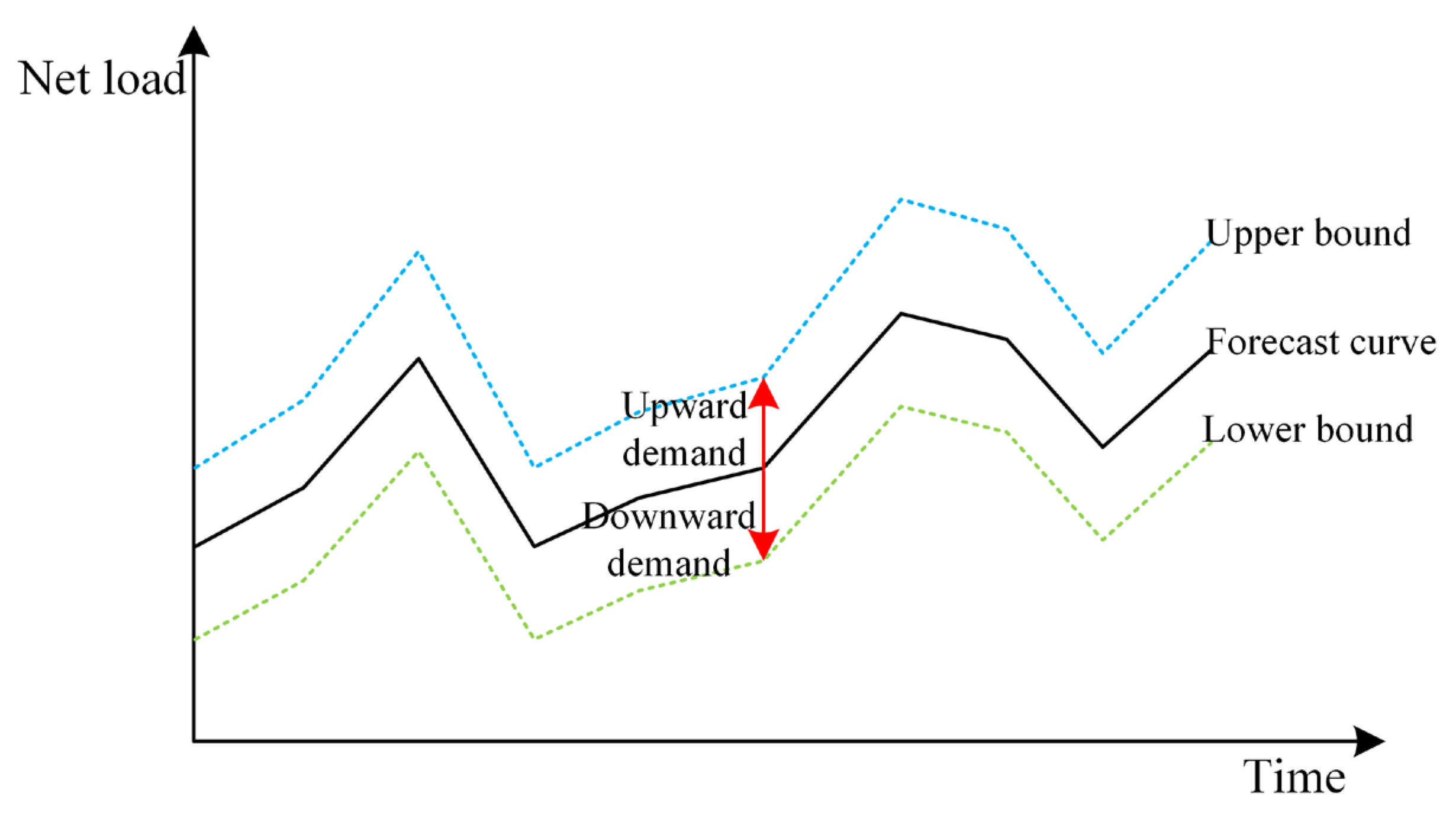
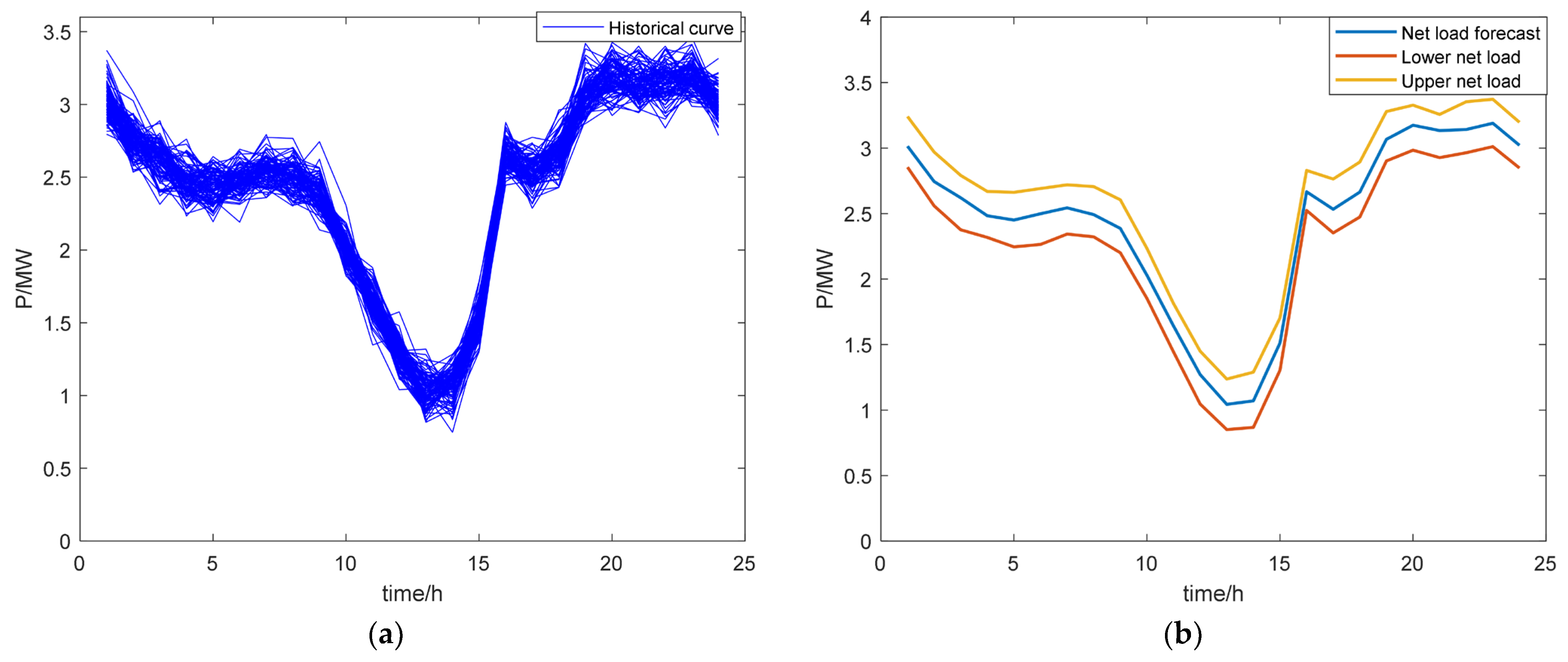
3.1. Mathematical Model of Net Load Uncertainty

The net load of the power system is defined as the difference between the load curve and the renewable energy generation curve. It is used to describe the load demand other than the new energy required by the power system over some time. It can help the power dispatch department to forecast and plan the power supply and demand and rationally arrange the power production, transmission, and distribution capacity to ensure the stable operation of the system. The net load formula in this paper is as follows:

$$P_t^{\mathrm{NL}}=P_t^{\mathrm{L}}-P_t^{\mathrm{RE}}$$

(26)

where $P_t^{\mathrm{NL}}$ is the value of the net load at time $t$; $P_t^{\mathrm{L}}$ is the value of the load at time $t$; $P_t^{\mathrm{RE}}$ is the value of new energy at time $t$.

Both load and new energy sources have uncertainty, and the uncertainty is greater in the day-ahead optimization, so we select multiple net load curves from historical data. Each period estimates its net load distribution using KDE, and the upper and lower bounds of the net load forecast curves are calculated by setting appropriate confidence intervals.

As shown in Figure 2, after deriving the KDE at different times, appropriate confidence intervals are chosen, and finally, the upper bound $Z_{\alpha }$ and lower bound $Z_{-\alpha }$ are derived.

After traversing all the time nodes, the upper and lower bounds of the net load forecast curve can be derived as shown in Figure 3.

Therefore, we need to integrate flexible resources to meet the uncertainty of load and new energy fluctuations. The uncertain fluctuation model is as follows.

$$\left\{\begin{array}{l}\Delta P_t^{\mathrm{NL},\mathrm{up}}=P_t^{\mathrm{NL},\mathrm{up}}-P_t^{\mathrm{NL}}\\ \Delta P_t^{\mathrm{NL},\mathrm{dn}}=P_t^{\mathrm{NL}}-P_t^{\mathrm{NL},\mathrm{dn}}\end{array}\right.$$

(27)

where $\Delta P_t^{\mathrm{NL},\mathrm{up}}$ is the upward demand at time $t$; $\Delta P_t^{\mathrm{NL},\mathrm{dn}}$ is the downward demand at time $t$; $P_t^{\mathrm{NL},\mathrm{up}}$ is the upper bound of the net load fluctuation at time $t$; $P_t^{\mathrm{NL},\mathrm{dn}}$ is the lower bound of the net load fluctuation at time $t$; and $P_t^{\mathrm{NL}}$ is the net load forecast at time $t$.

3.2. Model of Flexible Resources

In this paper, the ESA and the resource supply from the regional grid are considered. Aggregate $m$ is accessed in node $j$, and subsequent optimal scheduling uses the $j$ notation.

$$\left\{\begin{array}{l}{F}_t^{\mathrm{Tot},\mathrm{up}}={\displaystyle \sum _{j\in {\mathsf{\Omega }}_{\mathrm{ESSA}}}{F}_{j,t}^{\mathrm{ESSA},\mathrm{up}}}+F_t^{\mathrm{Grid},\mathrm{up}}\\ F_t^{\mathrm{Tot},\mathrm{dn}}={\displaystyle \sum _{j\in {\mathsf{\Omega }}_{\mathrm{ESSA}}}{F}_{j,t}^{\mathrm{ESSA},\mathrm{dn}}}+F_t^{\mathrm{Grid},\mathrm{dn}}\end{array}\right.$$

(28)

where $F_t^{\mathrm{Tot},\mathrm{up}}$ and $F_t^{\mathrm{Tot},\mathrm{dn}}$ are the sum of the system’s flexibility upward and downward resources at time $t$; $F_{j,t}^{\mathrm{ESSA},\mathrm{up}}$ and $F_{j,t}^{\mathrm{ESSA},\mathrm{dn}}$ are the flexibility upward and downward of the ESA $j$ at time $t$; $F_t^{\mathrm{Grid},\mathrm{up}}$ and $F_t^{\mathrm{Grid},\mathrm{dn}}$ are the flexibility upward and downward of the grid at time $t$.

(1)

Supply of ESA

$$\left\{\begin{array}{l}{F}_{j,t}^{\mathrm{ESA},\mathrm{up}}=\min (P_{j,t}^{\mathrm{dchA},\max }-P_{j,t}^{\mathrm{ESA}},(E_{j,t}^{\mathrm{A}}-E_{j,t}^{\mathrm{A},\min }){\eta }_j^{\mathrm{A},\mathrm{dch}}/\Delta t)\\ F_{j,t}^{\mathrm{ESA},\mathrm{dn}}=\min (P_{j,t}^{\mathrm{chA},\max }+P_{j,t}^{\mathrm{ESA}},(E_{j,t}^{\mathrm{A},\max }-E_{j,t}^{\mathrm{A}})/{\eta }_j^{\mathrm{A},\mathrm{ch}}\Delta t)\end{array}\right.$$

(29)

where $P_{j,t}^{\mathrm{ESA}}$ is the active power of the ESA $j$ at time $t$; $E_{j,t}^{\mathrm{A}}$ is the battery capacity of ESA $j$ at time $t$; ${\eta }_j^{\mathrm{A},\mathrm{ch}}$ and ${\eta }_j^{\mathrm{A},\mathrm{dch}}$ are the charging and discharging power factors of the ESA $j$, respectively.

(2)

Supply of regional grid

$$\left\{\begin{array}{l}{F}_t^{\mathrm{Grid},\mathrm{up}}=P^{\mathrm{Grid},\max }-P_t^{\mathrm{Grid}}\\ F_t^{\mathrm{Grid},\mathrm{dn}}=P_t^{\mathrm{Grid}}-P^{\mathrm{Grid},\min }\end{array}\right.$$

(30)

where $P_t^{\mathrm{Grid}}$ is the active power of power purchased from the regional grid at time $t$.

Therefore, the prediction uncertainty fluctuation balance mechanism is:

$$\left\{\begin{array}{l}\Delta D_t^{\mathrm{up}}=F_t^{\mathrm{Tot},\mathrm{up}}-\Delta P_t^{\mathrm{NL},\mathrm{up}}\hfill \\ \Delta D_t^{\mathrm{dn}}=F_t^{\mathrm{Tot},\mathrm{dn}}-\Delta P_t^{\mathrm{NL},\mathrm{dn}}\hfill \end{array}\right.$$

(31)

where $\Delta D_t^{\mathrm{up}}$ and $\Delta D_t^{\mathrm{dn}}$ are the flexibility upward and downward supply–demand balances at time $t$. The value is greater than 0 when the flexibility supply is considered to satisfy the uncertainty of demand fluctuation.

4. Day-Ahead Distribution Network Optimization Considering Aggregation and Uncertainty

4.1. Objective Function

To ensure the economic operation of the distribution network, the day-ahead optimization takes the cost of PVA, ESA, and power purchase from the regional grid as an objective function.

$$\min f=C^{\mathrm{PVA}}+C^{\mathrm{ESA}}+C^{\mathrm{Grid}}$$

(32)

where $C^{\mathrm{PVA}}$ is the PVA dispatch cost, $C^{\mathrm{ESA}}$ is the ESA dispatch cost, and $C^{\mathrm{Grid}}$ is the power purchase cost of the regional grid.

(1)

PVA dispatch cost

$$C^{\mathrm{PVA}}={\displaystyle \sum _{t=1}^T{\displaystyle \sum _{j\in {\mathsf{\Omega }}_{\mathrm{PVA}}}{c}_t^{\mathrm{PVA},\mathrm{Q}}{Q}_{j,t}^{\mathrm{PVA}}}}$$

(33)

where $c_t^{\mathrm{PVA},\mathrm{Q}}$ is the price of PVA reactive power dispatch at time $t$; $Q_{j,t}^{\mathrm{PVA}}$ is the reactive output of PVA $j$ at time $t$.

(2)

ESA dispatch cost

$$C^{\mathrm{ESA}}={\displaystyle \sum _{t=1}^T{\displaystyle \sum _{j\in {\mathsf{\Omega }}_{\mathrm{ESSA}}}(c_t^{\mathrm{ESA},\mathrm{P}}{P}_{j,t}^{\mathrm{ESA}}}}+c_t^{\mathrm{ESA},\mathrm{Q}}{Q}_{j,t}^{\mathrm{ESA}})$$

(34)

where $c_t^{\mathrm{ESA},\mathrm{P}}$ is the price of ESAs active dispatch at time $t$; $P_{j,t}^{\mathrm{ESA}}$ is the active output of ESA $j$ at time $t$; $c_t^{\mathrm{ESA},\mathrm{Q}}$ is the price of ESAs reactive dispatch at time $t$; $Q_{j,t}^{\mathrm{ESA}}$ is the reactive output of ESA $j$ at time $t$.

(3)

Power purchase cost from the regional grid

$$C^{\mathrm{Grid}}={\displaystyle \sum _{t=1}^T(c_t^{\mathrm{Grid},\mathrm{P}}{P}_t^{\mathrm{Grid}}+}{c}_t^{\mathrm{Grid},\mathrm{Q}}{Q}_t^{\mathrm{Grid}})$$

(35)

where $c_t^{\mathrm{Grid},\mathrm{P}}$ is the purchase price of active power from the regional grid at time $t$; $P_t^{\mathrm{Grid}}$ is the active power purchased by the grid from the regional grid at time $t$; $c_t^{\mathrm{Grid},\mathrm{Q}}$ is the purchase price of reactive power from the regional grid at time $t$; $Q_t^{\mathrm{Grid}}$ is the reactive power purchased by the grid from the regional grid at time $t$.

4.2. Constraints

Constraints include PVA operational constraints, ESA operational constraints, power constraints on regional grid contact lines, supply and demand balance constraints, and power system flow constraints.

(1)

PVA operational constraints

PVA active and reactive power constraints ensure the feasibility of scheduling and disaggregation.

$$\left\{\begin{array}{l}{P}_{j,t}^{\mathrm{PVA}}=P_{j,t}^{\mathrm{PVA},\mathrm{pre}}\\ \sqrt{{(P_{j,t}^{\mathrm{PVA}})}^2+{(Q_{j,t}^{\mathrm{PVA}})}^2}\le S_j^{\mathrm{PVA}}\end{array}\right.$$

(36)

where $P_{j,t}^{\mathrm{PVA},\mathrm{pre}}$ is the predicted active power of the PVA $j$ at time $t$, $P_{j,t}^{\mathrm{PVA}}$ is the active power of PVA $j$ at time $t$, $S_{j,t}^{\mathrm{PVA}}$ is the apparent power of the PVA $j$.

(2)

ESA operational constraints

ESA active power, reactive power, and battery capacity constraints ensure scheduling feasibility and aggregation decomposition of aggregates.

$$\left\{\begin{array}{l}{P}_{j,t}^{\mathrm{chA},\min }\le P_{j,t}^{\mathrm{chA}}\le P_{j,t}^{\mathrm{chA},\max }\\ P_{j,t}^{\mathrm{dchA},\min }\le P_{j,t}^{\mathrm{dchA}}\le P_{j,t}^{\mathrm{dchA},\max }\\ E_{j,t+1}^{\mathrm{A}}=E_{j,t}^{\mathrm{A}}+({\eta }_j^{\mathrm{chA}}{P}_{j,t}^{\mathrm{chA}}-{\displaystyle \frac{P_{j,t}^{\mathrm{dchA}}}{{\eta }_j^{\mathrm{dchA}}}})\Delta t\\ E_{j,t}^{\mathrm{A},\min }\le E_{j,t}^{\mathrm{A}}\le E_{j,t}^{\mathrm{A},\max }\\ P_{j,t}^{\mathrm{ESA}}=P_{j,t}^{\mathrm{dchA}}-P_{j,t}^{\mathrm{chA}}\\ \sqrt{{(P_{j,t}^{\mathrm{ESA}})}^2+{(Q_{j,t}^{\mathrm{ESA}})}^2}\le S_j^{\mathrm{ESA}}\end{array}\right.$$

(37)

(3)

Power constraints on regional grid tie lines

The active and reactive power constraints of the higher-level grid ensure that the power of the higher-level grid contact line is within the scheduling range.

$$\left\{\begin{array}{l}{P}^{\mathrm{Grid},\min }⩽P_t^{\mathrm{Grid}}⩽P^{\mathrm{Grid},\max }\\ Q^{\mathrm{Grid},\min }⩽Q_t^{\mathrm{Grid}}⩽Q^{\mathrm{Grid},\max }\end{array}\right.$$

(38)

where $P^{\mathrm{Grid},\min }$ and $P^{\mathrm{Grid},\max }$ are the minimum and maximum of the active power purchased from the regional grid, and $Q^{\mathrm{Grid},\min }$ and $Q^{\mathrm{Grid},\max }$ are the minimum and maximum of the reactive power purchased from the regional grid, respectively.

(4)

Supply and demand balance constraints

Based on the supply and demand balance constraints derived in Section 3, the supply and demand balance of active power in the network is guaranteed during the distribution network scheduling hours.

By deriving from Equations (26)–(31), additional constraints can be obtained, that is,

$$\left\{\begin{array}{l}\Delta D_t^{\mathrm{up}}\ge 0\hfill \\ \Delta D_t^{\mathrm{dn}}\ge 0\hfill \end{array}\right.$$

(39)

(5)

Power system flow constraints

Power flow constraints ensure that the distribution network is scheduled to operate with power, voltage, and electricity within allowable limits.

$$\left\{\begin{array}{l}{\displaystyle \sum _{i\in u(i)}(P_{ij,t}-r_{ij}{(I_{ij,t})}^2)}+P_{j,t}={\displaystyle \sum _{k\in v(j)}{P}_{jk,t}}\\ {\displaystyle \sum _{i\in u(i)}(Q_{ij,t}-x_{ij}{(I_{ij,t})}^2)}+Q_{j,t}={\displaystyle \sum _{k\in v(j)}{Q}_{jk,t}}\\ {(V_{j,t})}^2={(V_{i,t})}^2-2(r_{ij}{P}_{ij,t}+x_{ij}{Q}_{ij,t})+(r_{ij}^2+x_{ij}^2){(I_{ij,t})}^2\\ P_{j,t}=P_{j,t}^{\mathrm{ESSA}}+P_{j,t}^{\mathrm{PVA}}-P_{j,t}^{\mathrm{L}}\\ Q_{j,t}=Q_{j,t}^{\mathrm{ESSA}}+Q_{j,t}^{\mathrm{PVA}}-Q_{j,t}^{\mathrm{L}}\\ {(I_{ij,t})}^2={\displaystyle \frac{{(P_{ij,t})}^2+{(Q_{ij,t})}^2}{{(V_{j,t})}^2}}\\ {(V^{\min })}^2\le {(V_{j,t})}^2\le {(V^{\max })}^2\\ {(I_{ij,t})}^2\le {(I_{ij}^{\max })}^2\end{array}\right.$$

(40)

where $u(j)$ is the set of nodes flowing into $j$; $v(j)$ is the set of nodes flowing out from $j$; $P_{ij,t}$ and $Q_{ij,t}$ are the active and reactive power of node $i$ flowing to $j$ at time $t$, respectively; $P_{j,t}$ and $Q_{j,t}$ are the active and reactive power injected by node $j$ at time $t$, respectively; $V_{j,t}$ and $V_{i,t}$ are the actual voltage of node $j$ and node $i$ at time $t$; $r_{ij}$ and $x_{ij}$ are the resistance reactance of the branch $ij$, respectively; $I_{ij,t}$ is the current flowing between nodes $ij$; $V^{\max }$ and $V^{\min }$ are the upper and lower limits of voltage, respectively; $I_{ij}^{\max }$ is the maximum value of current.

Let $l_{ij,t}$ be equal to ${(I_{ij,t})}^2$ and $u_{j,t}$ be equal to ${(V_{j,t})}^2$ to perform second-order cone relaxation:

$$\left\{\begin{array}{l}{\displaystyle \sum _{i\in u(j)}(P_{ij,t}-r_{ij}{l}_{ij,t})}+P_{j,t}={\displaystyle \sum _{k\in v(j)}{P}_{jk,t}}\\ {\displaystyle \sum _{i\in u(j)}(Q_{ij,t}-x_{ij}{l}_{ij,t})}+Q_{j,t}={\displaystyle \sum _{k\in v(j)}{Q}_{jk,t}}\\ u_{j,t}=u_{i,t}-2(r_{ij}{P}_{ij,t}+x_{ij}{Q}_{ij,t})+(r_{ij}^2+x_{ij}^2)l_{ij,t}\\ l_{ij,t}{u}_{j,t}={(P_{ij,t})}^2+{(Q_{ij,t})}^2\\ {(V_j^{\min })}^2\le u_{j,t}\le {(V_j^{\max })}^2\\ l_{ij,t}\le {(I_{ij}^{\max })}^2\end{array}\right.$$

(41)

Further simplification leads to:

$$l_{ij,t}\ge {\displaystyle \frac{{(P_{ij,t})}^2+{(Q_{ij,t})}^2}{u_{j,t}}}\iff {‖\begin{array}{c}2P_{ij,t}\\ 2Q_{ij,t}\\ l_{ij,t}-u_{j,t}\end{array}‖}_2\le l_{ij,t}+u_{j,t}$$

(42)

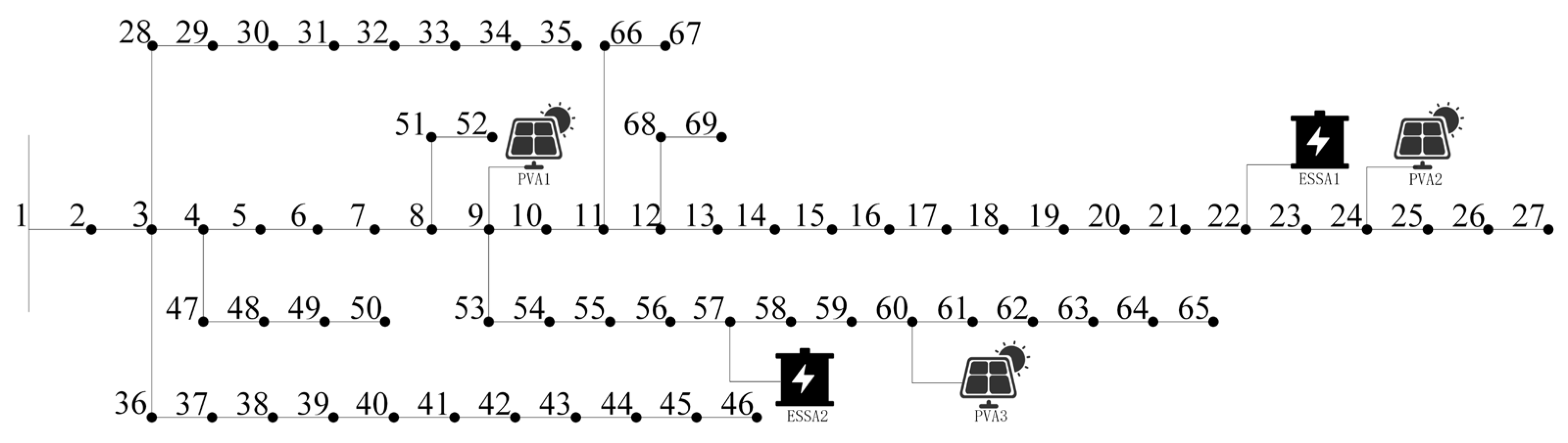
5. Case Study

In this paper, the IEEE 69-node distribution system is selected, and three PVAs and two ESAs are in the distribution network. This paper aims to verify the feasibility of the PV and ES aggregation methods and optimal dispatch. The test cases were conducted on a laptop with Intel Core i7-8550U CPU, 1.80 GHz and 16 GB RAM. The MATLAB R2023a software with YALMIP toolbox and CPLEX solver were used to solve the optimization problems.

5.1. PV and ES Aggregate Results

Selection of suitable PV unit and ES unit data and their aggregation and analysis.

(1)

PV aggregate results

The data for PV units are shown in

Table 1. PV unit data.

PV Unit	Rated Power/kW
PV 1	100
PV 2	200
PV 3	300
PV 4	400

.

Based on the rated power data of the PV units in Table 1, Minkowski power aggregation was performed to obtain the active and reactive power aggregation range of the PVA. The PVA feasible region is shown in the following figure.

As shown in Figure 4, Figure 4a indicates that the PVA power can be determined through Minkowski summation of the feasible regions of active and reactive power for PV units. Figure 4b indicates that by combining this active and reactive output with the PV forecast curves, the actual PV output can be accurately derived, and further scheduling optimization solutions can follow.

(2)

ES aggregate results

Among them, the types of ES units are shown in the following

Table 2. ES unit data.

ES Unit	Rated Power/kW	Rated Capacity/kWh
ES 1	100	550
ES 2	150	600
ES 3	200	650

.

The following three ES aggregate and optimal scheduling examples are set up for comparative analysis:

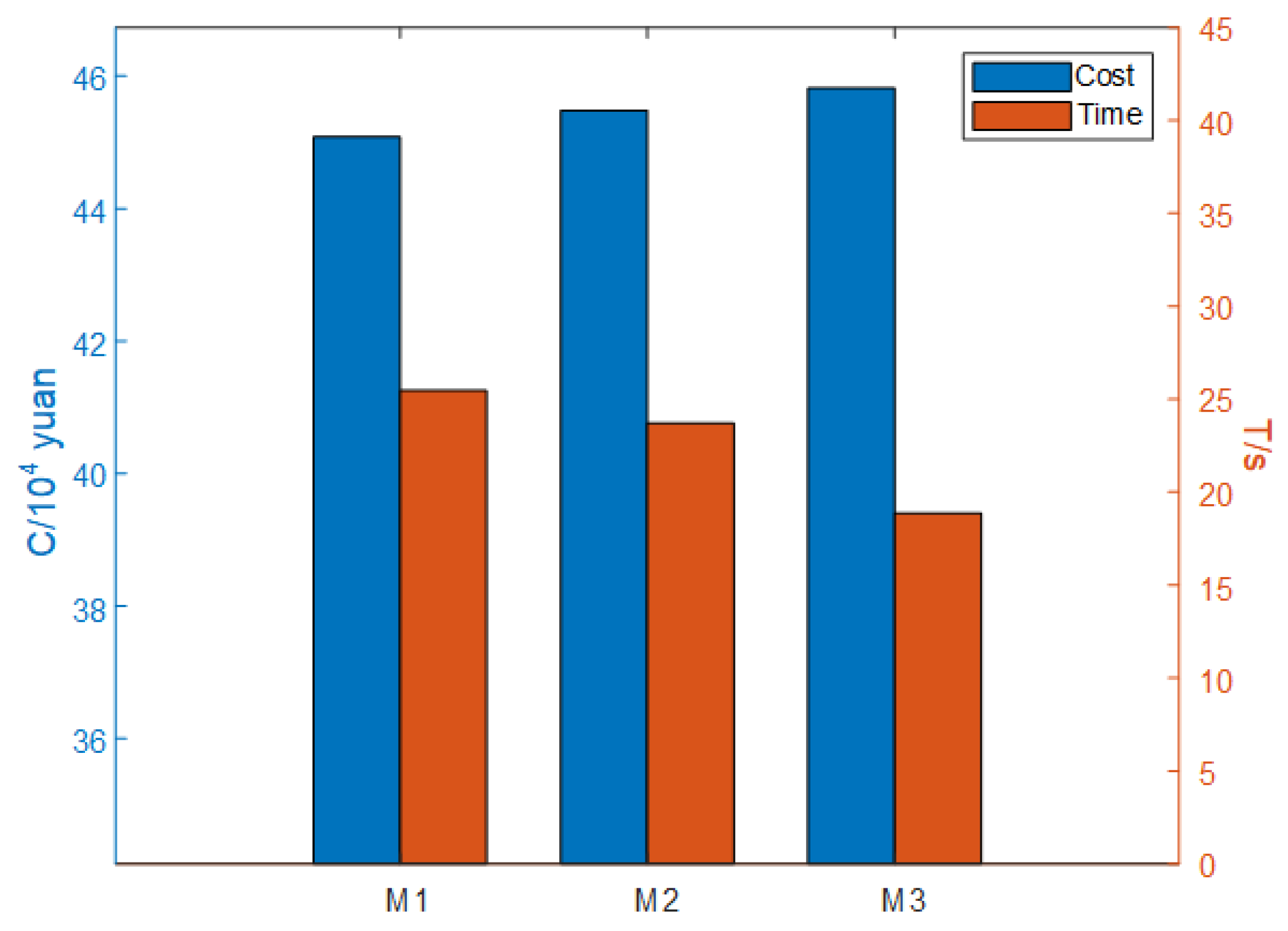
• Method 1 (M1): Original optimal scheduling without using the aggregation method;
• Method 2 (M2): Proposed method, Minkowski summation and polytope inner approximation for aggregation optimal scheduling;
• Method 3 (M3): Box inner approximate method [28] for aggregation optimal scheduling.

The ESA’s AFR is shown in Figure 5:

Figure 5 shows the active power feasible region and battery capacity range for different aggregate methods and the original method, where the ES active power is equal to the discharge power minus the charge power.

It can be seen that the difference between M1 and M2 in this paper is not much, losing part of the feasible region. As for the feasible region of M3, most of the feasible domain is lost due to the decoupling of active power and battery capacity, and the results are more conservative.

Figure 6 shows the effectiveness of the M2 method of aggregation, which is further verified by comparing the active and reactive power feasible regions of the different methods. It can be seen that at time t1, the active and reactive power feasible region after M2 aggregation is approximated as the M1 feasible region, with only a small part of the feasible region lost, while the feasible region of M3 is a strip-shaped region, with most of the active and reactive power feasible region lost.

Thus, further evidence of the aggregate region effect of the polytope inner approximate methods is needed in this paper.

5.2. Distribution Network Day-Ahead Optimization Results

In this paper, we take the IEEE 69-node as an example with data from reference [29], whose topology is shown in Figure 7 where three PVAs and two ESAs were set up. The PVA1, PVA2, PVA3, ESSA1 and ESSA2’s active power and reactive power feasible regions are obtained after aggregating by the above aggregate methods. The placing of PVAs and ESAs is determined by a combination of interdependent factors: (i) load distribution patterns and voltage regulation demands; (ii) spatiotemporal characteristics of renewable energy resources; (iii) network topology constraints and congestion mitigation strategies; and (iv) practical engineering requirements derived from specific application scenarios.

Time-of-day tariffs refer to the division of a 24 h day into periods according to the operating conditions of the system, with each period being charged at the average marginal cost of system operation. Time-of-use tariffs stimulate and encourage electricity consumers to shift peaks and valleys and optimize electricity consumption. Each day is divided into three tariffs, with each tariff specifically delineated according to the respective season and the time when peak and valley loads occur. This paper delineates 7 h for the peak period, 5 h for the trough period, and 12 h for the average period. Therefore, this paper calculates the regulation cost of the flexibility resources, taking into account the real-time impact of time-of-day tariffs, which makes the cost of the flexibility resources more accurate, and the time-of-day tariffs are shown in

Table 3. Time-of-day tariffs.

Time	Time-of-Day Tariff Ratio/CNY/kWh
00:00–05:00	0.3
05:00–09:00	0.6
9:00–12:00	0.9
12:00–16:00	0.6
16:00–20:00	0.9
20:00–24:00	0.6

.

(1)

Flexibility in supply and demand balance

As shown in Figure 8, first, 100 net load historical data curves were derived from the statistical data. Then, based on the historical data, the kernel estimation method was used to derive the upper and lower net load limits. Finally, the net load forecast curves wee combined to derive flexibility demand upper and lower bound values for subsequent optimal scheduling.

(2)

Distribution network optimization

We performed a comparative analysis of flexibility resource availability, economics, and solution speed after optimal scheduling.

Figure 9 shows that the flexibility of M1 optimized scheduling and M2 is adjusted upward and downward by similar magnitudes, with M2 being smaller than M1 optimized scheduling only at individual times. The optimal scheduling of M3 is much smaller than the optimal scheduling of M1 and the optimal scheduling of M2 in terms of the overall flexibility of upward and downward adjustments.

Therefore, in this paper, we assert that the resource flexibility adjustment capability, following the polytope inner approximation, is significantly enhanced when it is incorporated into the optimal scheduling framework of the power system. This implies that the approximation process not only provides a more accurate representation of the resource flexibility but also ensures that the system’s operational efficiency and robustness are optimized through the scheduling process.

Figure 10 compares the cost and computation time of different optimal scheduling methods. It can be seen that M1 scheduling has the minimum cost but the maximum computation time. In comparison, M3 has the maximum cost but the minimum computation time. And M1 has relatively better cost and faster computation time. If the number of aggregate units increases, the cost, computation time, and feasible region of the polytope inner approximation optimal scheduling method in this paper will further highlight its superiority.

Table 4. Comparison of examples.

Flexibility	Optimization Cost	Computation Time
M1 > M2 > M3	M3 > M2 > M1	M1 > M2 > M3

shows a comparison of the flexibility, optimization cost and computation time effects of the three aggregation and scheduling schemes.

In summary, the proposed M2 method demonstrates comprehensive superiority across key performance metrics: compared to the M3 approach, it achieves enhanced aggregation efficacy by better preserving resource flexibility characteristics while maintaining tighter operational boundaries; economically, M2 outperforms M3 through improved cost-efficiency ratios in scheduling decisions; and regarding computational performance, M2 exhibits significantly faster solution speeds than the baseline M1 unaggregated scheduling scheme. The tripartite advantages of the M2 approach in terms of aggregation effectiveness, economic optimization, and computational efficiency make it a well-balanced solution that simultaneously addresses the key challenges of model aggregation computation, operational cost, and real-time dispatch feasibility in modern power systems.

Figure 11 presents the optimal scheduling outcomes for PV and ES obtained through the M2 optimization methodology. The PV reactive power scheduling results show that more reactive power scheduling is needed at noon, that there is sufficient reactive power in the network, and that the overall PV reactive power demand is not too large.

The ES active power, reactive power, and battery state of charge (SOC) scheduling results show that charging is performed in the early morning hours when the tariff is relatively low, the network has sufficient active power storage in the daytime hours to serve, relatively, as a standby flexibility resource, and the ES active power discharges more to supply the network at night. Reactive power utilization is relatively low due to sufficient network reactive power. Battery capacity is charged in the morning, fully charged as a standby flexibility resource, and discharged at night to supply the network.

(3)

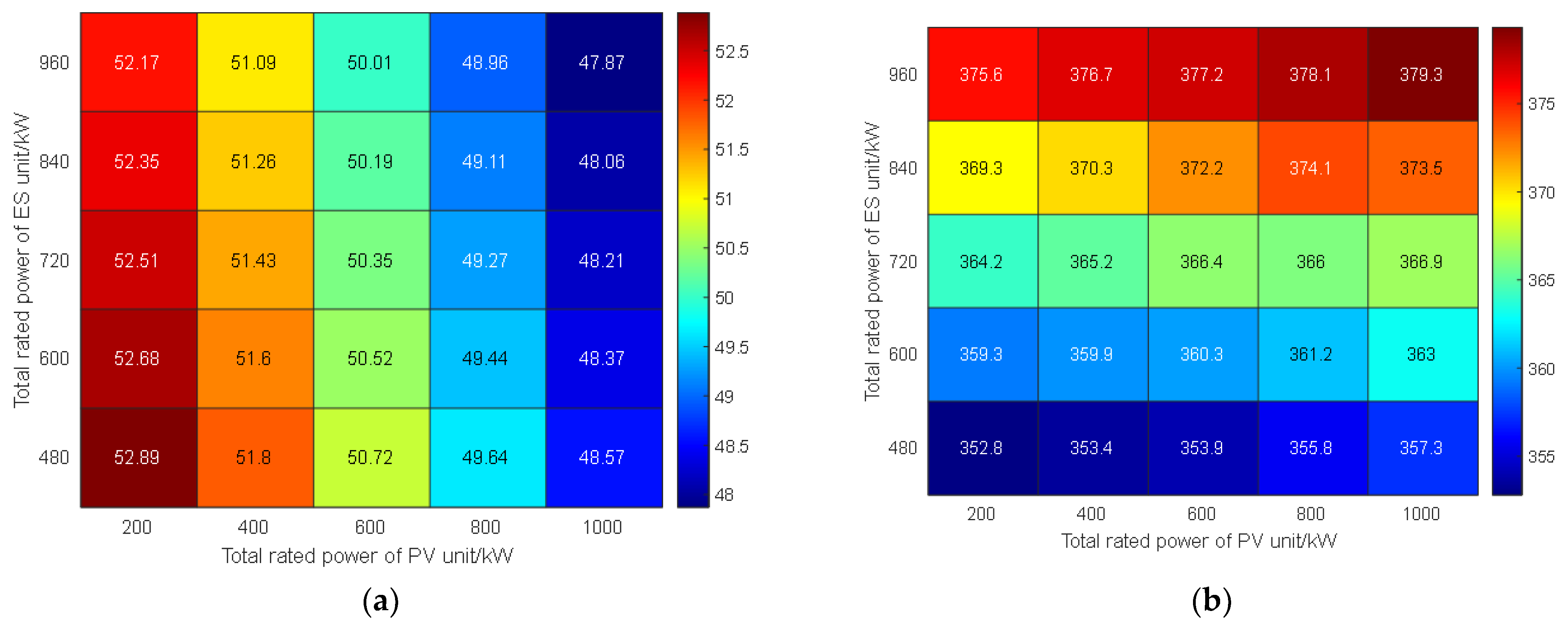
Sensitivity analysis

By changing the PV units’ power rating and ES units’ power rating parameters, the aggregation and optimization solution is performed to analyze the optimization target cost (CNY 10⁴) and flexibility margin (MW).

As illustrated in Figure 12a, the system exhibits distinct cost reduction patterns: the cost of system optimization tends to decrease as PV penetration increases, while the cost of ESS likewise decreases as ESS integration capabilities increase. Figure 12b reveals a coupled optimization mechanism where enhanced PV not only reduces overall system costs but also improves operational flexibility, with ESS integration further amplifying this flexibility enhancement. Both PV and ESS power ratings exhibit strong positive correlations with the dual optimization objectives, achieving cost effectiveness and maintaining sufficient flexibility margin for grid operation.

6. Conclusions

This paper focuses on proposing a bottom-up aggregation method for aggregating distributed PV and ES systems and then deriving scheduling results through up-bottom day-ahead optimal scheduling of the distribution network, while taking aggregation and uncertainty into account. The main conclusions are summarized as follows:

• The Minkowski summation method for PV systems and the polytope inner approximation method for ES are proposed. These methods effectively aggregate distributed PV and ES units into resource aggregators through mathematical modeling and algorithm design. Compared to the box inner approximation method, the AFR is enlarged, and the aggregation effect is more pronounced.
• To address the uncertainty in optimal scheduling, the KDE method is applied to transform the uncertainty problem into a deterministic flexibility supply–demand balance problem. This transformation not only simplifies the problem’s complexity but also enhances the robustness and flexibility of the model.
• A distribution network optimal scheduling model considering aggregate distributed resources and uncertainty is developed. This model accounts for the aggregation characteristics of distributed resources as well as various uncertainty factors. Comparative analysis shows that the proposed method outperforms the box inner approximation aggregation optimization method and provides faster solutions than the original optimization approach, resulting in more scientifically grounded and reasonable scheduling outcomes.

In future work, the aggregation of additional distributed resources into a single resource aggregator will be explored. Moreover, multi-objective optimization, considering both the distribution network and aggregator objectives, will be incorporated into subsequent optimal scheduling efforts.

References

- Çiçek, A.; Erdinç, O. Risk-averse optimal bidding strategy for a wind energy portfolio manager including EV parking lots for imbalance mitigation. Turk. J. Electr. Eng. Comput. Sci. 2021, 29, 481–498. [Google Scholar] [CrossRef]
- Wen, Y.; Hu, Z.; You, S.; Duan, X. Aggregate feasible region of DERs: Exact formulation and approximate models. IEEE Trans. Smart Grid 2022, 13, 4405–4423. [Google Scholar] [CrossRef]
- Taheri, S.; Kekatos, V.; Veeramachaneni, S.; Zhang, B. Data-driven modeling of aggregate flexibility under uncertain and non-convex device models. IEEE Trans. Smart Grid 2022, 13, 4572–4582. [Google Scholar] [CrossRef]
- Tiwary, H.R. On the hardness of computing intersection, union and Minkowski sum of polytopes. Discret. Comput. Geom. 2008, 40, 469–479. [Google Scholar] [CrossRef]
- Van Tu, T. Minimal representations of a face of a convex polyhedron and some applications. Acta Math. Vietnam. 2021, 46, 761778. [Google Scholar] [CrossRef]
- Wang, X. Tri-Level scheduling model considering residential demand flexibility of aggregated HVACs and EVs under distribution LMP. IEEE Trans. Smart Grid 2021, 12, 3990–4002. [Google Scholar] [CrossRef]
- Zhou, M.; Wu, Z.; Wang, J.; Li, G. Forming dispatchable region of electric vehicle aggregation in microgrid bidding. IEEE Trans. Ind. Informat. 2021, 17, 4755–4765. [Google Scholar] [CrossRef]
- Hu, J.; Wu, J.; Ai, X.; Liu, N. Coordinated energy management of prosumers in a distribution system considering network congestion. IEEE Trans. Smart Grid 2021, 12, 468–478. [Google Scholar] [CrossRef]
- Barot, S.; Taylor, J.A. A concise, approximate representation of a collection of loads described by polytopes. Int. J. Electr. Power Energy Syst. 2017, 84, 55–63. [Google Scholar] [CrossRef]
- Pertl, M.; Carducci, F.; Tabone, M.; Marinelli, M.; Kiliccote, S.; Kara, E.C. An equivalent time-variant storage model to harness EV flexibility: Forecast and aggregation. IEEE Trans. Ind. Informat. 2019, 15, 1899–1910. [Google Scholar] [CrossRef]
- Chen, X.; Dall’Anese, E.; Zhao, C.; Li, N. Aggregate power flexibility in unbalanced distribution systems. IEEE Trans. Smart Grid 2020, 11, 258–269. [Google Scholar] [CrossRef]
- Yan, D.; Ma, C.; Chen, Y. Distributed coordination of charging stations considering aggregate EV power flexibility. IEEE Trans. Sustain. Energy 2023, 14, 356–370. [Google Scholar] [CrossRef]
- Müller, F.L.; Szabó, J.; Sundström, O.; Lygeros, J. Aggregation and disaggregation of energetic flexibility from distributed energy resources. IEEE Trans. Smart Grid 2019, 10, 1205–1214. [Google Scholar] [CrossRef]
- Hreinsson, K.; Scaglione, A.; Alizadeh, M.; Chen, Y. New insights from the Shapley-Folkman lemma on dispatchable demand in energy markets. IEEE Trans. Power Syst. 2021, 36, 4028–4041. [Google Scholar] [CrossRef]
- Zhao, L.; Zhang, W.; Hao, H.; Kalsi, K. A geometric approach to aggregate flexibility modeling of thermostatically controlled loads. IEEE Trans. Power Syst. 2017, 32, 4721–4731. [Google Scholar] [CrossRef]
- Yi, Z.; Xu, Y.; Gu, W.; Yang, L.; Sun, H. Aggregate operation model for numerous small-capacity distributed energy resources considering uncertainty. IEEE Trans. Smart Grid 2021, 12, 4208–4224. [Google Scholar] [CrossRef]
- Mangasarian, O.L. Set containment characterization. J. Global Optim. 2002, 24, 473–480. [Google Scholar] [CrossRef]
- Hao, H.; Sanandaji, B.M.; Poolla, K.; Vincent, T.L. Aggregate flexibility of thermostatically controlled loads. IEEE Trans. Power Syst. 2015, 30, 189–198. [Google Scholar] [CrossRef]
- Vagropoulos, S.I.; Bakirtzis, A.G. Optimal bidding strategy for electric vehicle aggregators in electricity markets. IEEE Trans. Power Syst. 2013, 28, 4031–4041. [Google Scholar] [CrossRef]
- Habibifar, R.; Lekvan, A.A.; Ehsan, M. A risk-constrained decision support tool for EV aggregators participating in energy and frequency regulation markets. Elect. Power Syst. Res. 2020, 185, 0378–7796. [Google Scholar] [CrossRef]
- Liang, H.; Liu, Y.; Li, F.; Shen, Y. Dynamic economic/emission dispatch including PEVs for peak shaving and valley filling. IEEE Trans. Ind. Electron. 2019, 66, 2880–2890. [Google Scholar] [CrossRef]
- Majzoobi, A.; Khodaei, A. Application of microgrids in supporting distribution grid flexibility. IEEE Trans. Power Syst. 2017, 32, 3660–3669. [Google Scholar] [CrossRef]
- Fang, X.; Misra, S.; Xue, G.; Yang, D. Smart grid—The new and improved power grid: A survey. IEEE Commun. Surv. Tuts. 2012, 14, 944–980. [Google Scholar] [CrossRef]
- Yang, X.; Xu, C.; He, H.; Yao, W.; Wen, J.; Zhang, Y. Flexibility provisions in active distribution networks with uncertainties. IEEE Trans. Sustain. Energy 2021, 12, 553–567. [Google Scholar] [CrossRef]
- Niu, H.; Yang, L.; Zhao, J.; Wang, Y.; Wang, W.; Liu, F. Flexible-regulation resources planning for distribution networks with a high penetration of renewable energy. IET Gener. Transm. Distrib. 2018, 12, 4099–4107. [Google Scholar]
- Wang, Q.; Hodge, B.M. Enhancing Power System Operational Flexibility with Flexible Ramping Products: A Review. IEEE Trans. Ind. Inform. 2017, 13, 1652–1664. [Google Scholar] [CrossRef]
- Hardy, G.H.; Littlewood, J.E.; Pólya, G. Inequalities, Cambridge Mathematical Library, 2nd ed.; Cambridge University Press: Cambridge, UK, 1952; pp. 35880–35889. [Google Scholar]
- Zhang, M.; Xu, Y.; Shi, X.; Guo, Q. A Fast Polytope-Based Approach for Aggregating Large-Scale Electric Vehicles in the Joint Market Under Uncertainty. IEEE Trans. Smart Grid 2024, 15, 701–713. [Google Scholar] [CrossRef]
- Jia, H.; Zhu, X.; Cao, W. Distribution Network Reconfiguration Based on an Improved Arithmetic Optimization Algorithm. Energies 2024, 17, 1969. [Google Scholar] [CrossRef]