Abstract
Within the spectrum of complex downhole operational challenges, pipe sticking incidents emerge as one of the most prevalent and costly drilling complications. These incidents characteristically develop through progressive deterioration rather than abrupt failure, with discernible precursor signals typically manifesting as anomalous patterns in critical drilling parameters (torque fluctuations, drag anomalies, deviations in standpipe pressure). Consequently, early detection of these signals plays a pivotal role in mitigating pipe sticking occurrences. To systematically investigate the characteristic signatures pipe sticking events, this study employs two modal decomposition methods to extract salient features from near-bit downhole data. Conventional pipe sticking prediction methodologies exhibit three predominant limitations: rule-based systems suffer from poor generalizability, physics-based models demonstrate low computational efficiency, and data-driven techniques lack physical interpretability. To overcome these constraints, this study innovatively proposes a physically constrained prediction framework that integrates Variational Mode Decomposition (VMD) with near-bit measurement data. Experimental results demonstrate the superior predictive capability of the proposed VMD-based, near-bit data-physical constraint model. Based on a comprehensive evaluation using six benchmark models, the proposed approach achieves optimal performance, with an R2 metric of approximately 0.9, significantly outperforming existing algorithms. When deployed in actual drilling operations, this model exhibits robust early detection of pipe sticking precursors, enabling proactive intervention. The practical implementation of this framework facilitates timely corrective actions, thereby substantially reducing the incidence of downhole pipe sticking events and enhancing operational safety.
1. Introduction
During the drilling process of unconventional reservoirs, complex downhole accidents are prone to occur, which can significantly affect drilling efficiency and operational safety [1,2]. As a predominant drilling non-productive time (NPT) contributor, stuck pipe events are invariably preceded by measurable parameter deviations, making early warning systems essential for risk mitigation. Existing prediction frameworks principally employ: (i) rule-based heuristics, (ii) physics-based simulations, or (iii) data-driven algorithms [3]. Nevertheless, these established approaches demonstrate fundamental constraints in either generalizability, computational efficiency, or physical interpretability.
Simple rule-based methods identify anomalies by analyzing the statistical characteristics of drilling parameters, such as standard deviation and skewness [4,5,6,7]. However, these methods fail to fully capture the complexity of stuck pipe incidents and require predefined thresholds, limiting their applicability. Physics-based methods, on the other hand, use physical models (e.g., torque and hydraulic models [8]) to detect stuck pipe signals by setting anomaly thresholds or estimating drilling variables [9,10,11]. However, the accuracy of these methods is highly dependent on input parameters, such as wellbore and drilling fluid properties, which often exhibit significant uncertainty [12]. Additionally, the parameter estimation process is challenging, especially when only surface data are available, which may lead to local solution issues. Data-driven methods, particularly machine learning techniques, offer the potential to predict stuck pipe incidents by learning abnormal patterns from historical data [13,14,15,16,17]. While supervised learning methods have been widely adopted, the scarcity of stuck pipe data makes them prone to overfitting, causing the models to focus more on the stuck events rather than the early warning signs. As a result, some studies have begun to explore unsupervised learning; however, the accuracy remains limited due to the insufficient data.
To overcome these issues, non-stationary signal processing methods have gained significant attention in recent years. These methods are particularly useful when the frequency components of a signal change over time. Traditional time-frequency transformation techniques, such as the Short-Time Fourier Transform (STFT) [18] and wavelet transform [19], are commonly employed for signal analysis. While these methods can separate signals in the time-frequency domain and perform multi-scale processing, they have limitations when handling non-stationary signals. For instance, the frequency resolution of STFT cannot be adjusted based on the signal characteristics, and wavelet transform tends to have relatively poor resolution in the low-frequency range.
To address these issues, Huang et al. [20] proposed the Empirical Mode Decomposition (EMD) method in 1988, which decomposes a signal into a set of Intrinsic Mode Functions (IMFs) [21] with different frequency components. EMD is particularly suitable for non-stationary and nonlinear vibration signals, and the instantaneous frequencies obtained through its decomposition have clear physical meanings [22]. Furthermore, Variational Mode Decomposition (VMD) was developed as an improvement over EMD. By solving an optimization problem, VMD extracts modes from the signal, thus avoiding the mode mixing problem inherent in EMD. VMD not only provides a more accurate representation of the frequency components in the signal but also offers greater adaptability and precision.
Based on the above analysis, this paper proposes a new method for predicting stuck pipe incidents. The method combines the feature extraction capabilities of modal decomposition with a hybrid approach of physical mechanisms and data-driven techniques, aiming to address the inherent limitations of previous methods. This hybrid approach enables more accurate identification of early signs of stuck pipe incidents and provides a more reliable prediction model for practical applications.
2. Algorithm Principles
2.1. Empirical Mode Decomposition
The Empirical Mode Decomposition (EMD) algorithm requires the input vibration signal x(t) to satisfy the fundamental Intrinsic Mode Function (IMF) condition, mandating the presence of at least two extrema (one maximum and one minimum). The local temporal characteristics of the signal are governed by the characteristic time scale τ defined by the inter-extrema intervals, which determines the instantaneous frequency components of the signal’s oscillatory modes. In the context of Empirical Mode Decomposition (EMD), for a vibration signal sequence x(t), it is assumed that the signal has at least two extreme points, one being a maximum and the other a minimum. The local time domain characteristics of the data sequence are uniquely determined by the time scale between extreme points. If the data sequence lacks extreme points but has inflection points, extreme points can be obtained by differentiating the data once or multiple times, and then the decomposition results can be obtained through integration. The process of Empirical Mode Decomposition [23] for the vibration signal x(t) is shown in Table 1.

Table 1.
The process of Empirical Mode Decomposition.
2.2. Variational Mode Decomposition
The specific decomposition process of VMD can be regarded as the solution to a variational problem, with the algorithm primarily involving the construction of the variational problem and its solution. The variational problem can be constructed in the following manner. For the k-th carbon emission modal component , the Hilbert transform is applied to obtain the analytic signal for each , and its one-sided spectrum can be calculated using the following equation [24]:
where represents the Dirac delta function; k denotes that the original carbon emission signal is composed of k carbon emission modal components ; j represents the imaginary unit. By multiplying Equation (1) with the exponential term corresponding to the central frequency of each carbon emission modal component , the spectra of the modes can be modulated to their respective basebands [25] according to Equation (2):
The 2-norm of the demodulated gradient is calculated using Equations (3) and (4), and the bandwidth of is estimated [26] as follows:
where represents the original complex carbon emission signal.
Based on this, the solution process of VMD mainly considers two constraints:
1. The sum of the bandwidths of each carbon emission mode component and its corresponding central frequency is minimized.
2. The sum of the k carbon emission mode components equals the original input complex carbon emission signal.
To solve the objective function represented by Equations (3) and (4), a quadratic penalty parameter α and a Lagrange multiplier operator are introduced into Equation (5). After introducing these two elements, the augmented Lagrangian function can be expressed as shown in Equation (5):
Then, the Alternating Direction Method of Multipliers (ADMM) is employed to solve Equation (5). After which, the optimal solution of the Lagrangian function is obtained as
where represents the expression of the carbon emission mode component , transformed from the time domain to the frequency domain using the Fourier transform; the same applies to and ; is the noise tolerance, and adjusting its value can reduce the impact of noise.
3. The Characteristics Analysis of Sticking
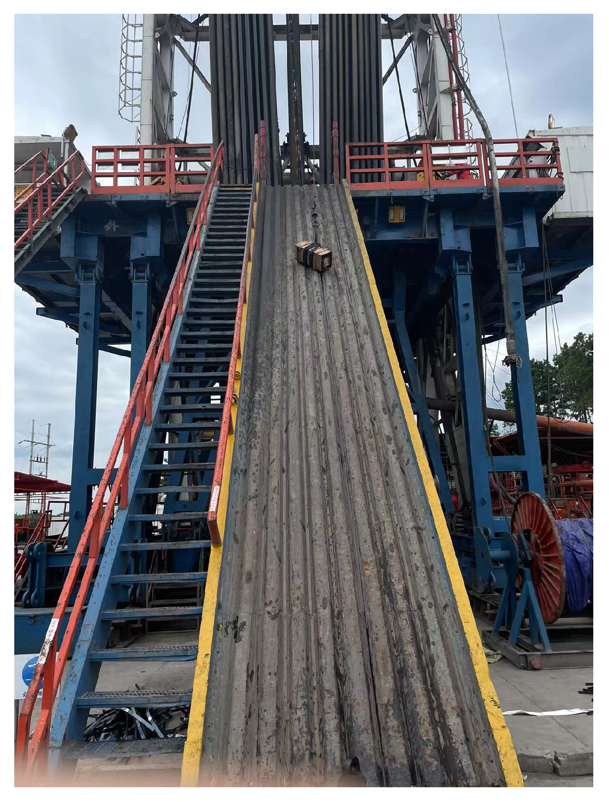
The data used in this study are derived from the downhole measurements of Well Wei202H23. The Wei202H23 platform, located in Group 9, Changling Village, Shanwang Town, Weiyuan County, Neijiang City, Sichuan Province, is depicted in Figure 1. The exploration and development rights for the area surrounding the Wei202H23 platform are held by PetroChina Company Limited. This task originates from the 2019 exploration and development well placement plan of the Sichuan Oil and Gas Project Manager Department. The platform serves as a horizontal well for the capacity construction of the Longmaxi Formation shale gas reservoir in the Wei202 well area.
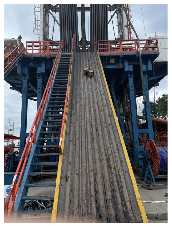
Figure 1.
We202H23-3 platform.
The data extracted covers a 5 min period, comparing the changes in parameters under normal drilling and stuck pipe conditions in the time domain, frequency domain, time-frequency domain, and vibration. The stuck pipe data include 3 min before the stuck pipe event and 2 min after the event, collectively forming the data for stuck pipe analysis. This study investigated a stuck pipe event that occurred during back-reaming, which was caused by borehole shrinkage and classified as mechanical sticking. In this study, the target wellbore for analysis is a vertical well, which should be considered when interpreting the applicability of the proposed predictive models.
3.1. Time Domain Analysis
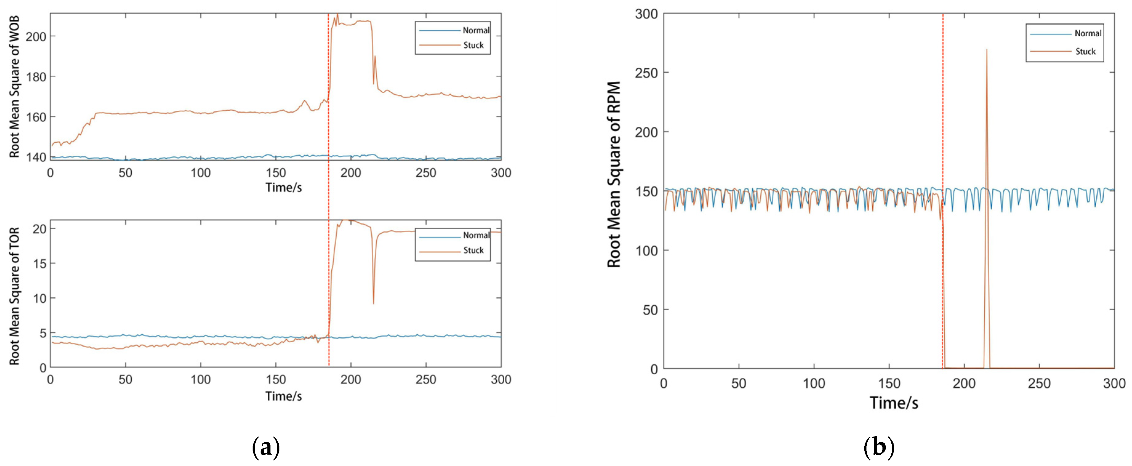
As shown in Figure 2, the analysis focuses on the root mean square (RMS) values of WOB (weight on bit, kN), TOR (torque, kN·m), and RPM (rotary speed, rev/min) under normal drilling and stuck pipe conditions. The RMS values can clearly reveal the characteristics of parameter changes when a stuck pipe event occurs. During normal drilling, the RMS values of WOB, TOR, and RPM remain stable. The moment a stuck pipe event occurs, the RMS value of RPM drops rapidly to 0. The RMS value of WOB increases from around 160 kN to near 200 kN, while the RMS value of TOR rises from 5 kN·m to 20 kN·m. Before the stuck pipe event occurs, only the WOB shows an increase compared to normal drilling conditions, rising from 145 kN to 160 kN in the 3 min prior to the stuck pipe event. The RMS values of TOR and RPM remain consistent with those during normal drilling, without any significant characteristics.
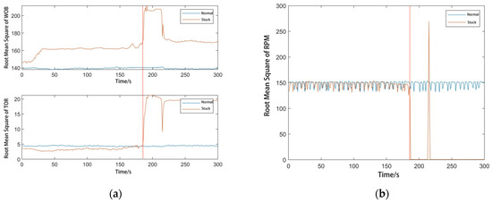
Figure 2.
Time domain analysis of near-bit data. (a) Root Mean Square of WOB and TOR; (b) Root Mean Square of RPM.
3.2. Frequency Domain Analysis
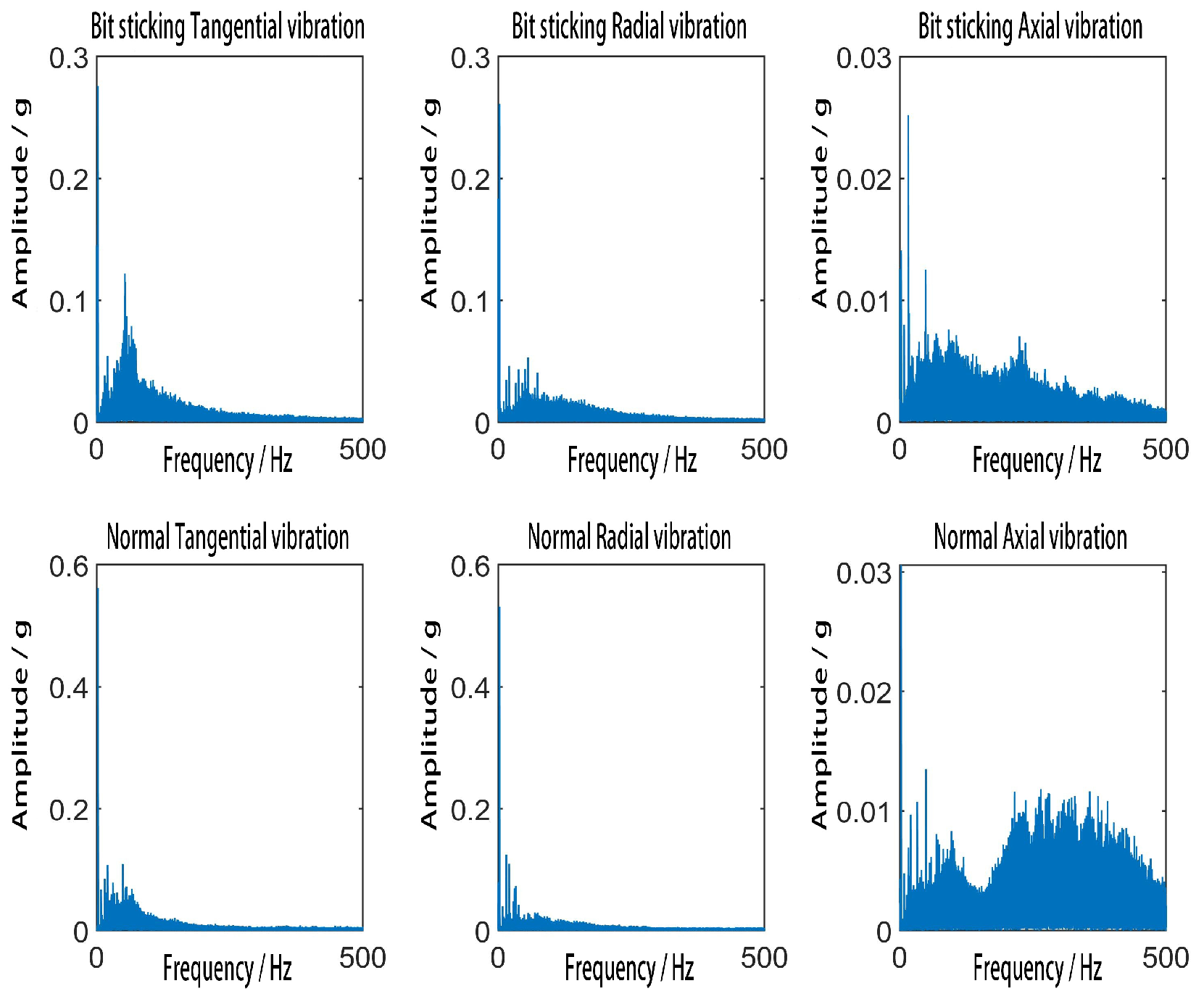
As shown in Figure 3, a comparison is made between tangential, radial, and axial vibrations under normal drilling and bit sticking conditions. During normal drilling, the amplitude of tangential vibration is within 0.2 g, radial vibration within 0.2 g, and axial vibration within 0.03 g, maintaining relatively stable vibration amplitudes. The frequencies of tangential, radial, and axial vibrations are primarily concentrated below 200 Hz. Before the occurrence of a stuck pipe event, the tangential, radial, and axial vibrations are similar to those observed during normal drilling, indicating no significant deviation. After the stuck pipe event, vibrational amplitudes significantly decrease, and the energy levels drop close to zero, suggesting vibration disappearance. Despite this, the frequency components of the signals remain mainly concentrated below 200 Hz.
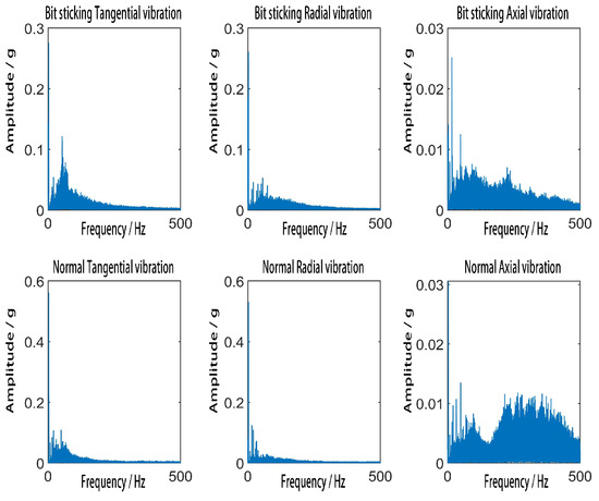
Figure 3.
Frequency domain analysis of near-bit data.
Figure 3 comparatively characterizes the tangential, radial, and axial vibration signatures under normal drilling and stuck pipe conditions. During normal drilling operations, vibration amplitudes remain stable, and spectral analysis shows that energy distribution for all vibration modes is predominantly within the sub-200 Hz range. During the pre-sticking phase, vibrational amplitudes do not show noticeable deviation from normal patterns. However, following the onset of sticking, the vibrational energy diminishes sharply while frequency domain features maintain concentrations below 200 Hz.
By comparing the parameter variations in the frequency domain under normal drilling and stuck pipe conditions, it is found that the parameter characteristics prior to the stuck pipe event are very similar to those during normal drilling. Therefore, it is difficult to extract distinguishing features before and after the stuck pipe event, making the early prediction of stuck pipe occurrences challenging.
3.3. Vibration Analysis
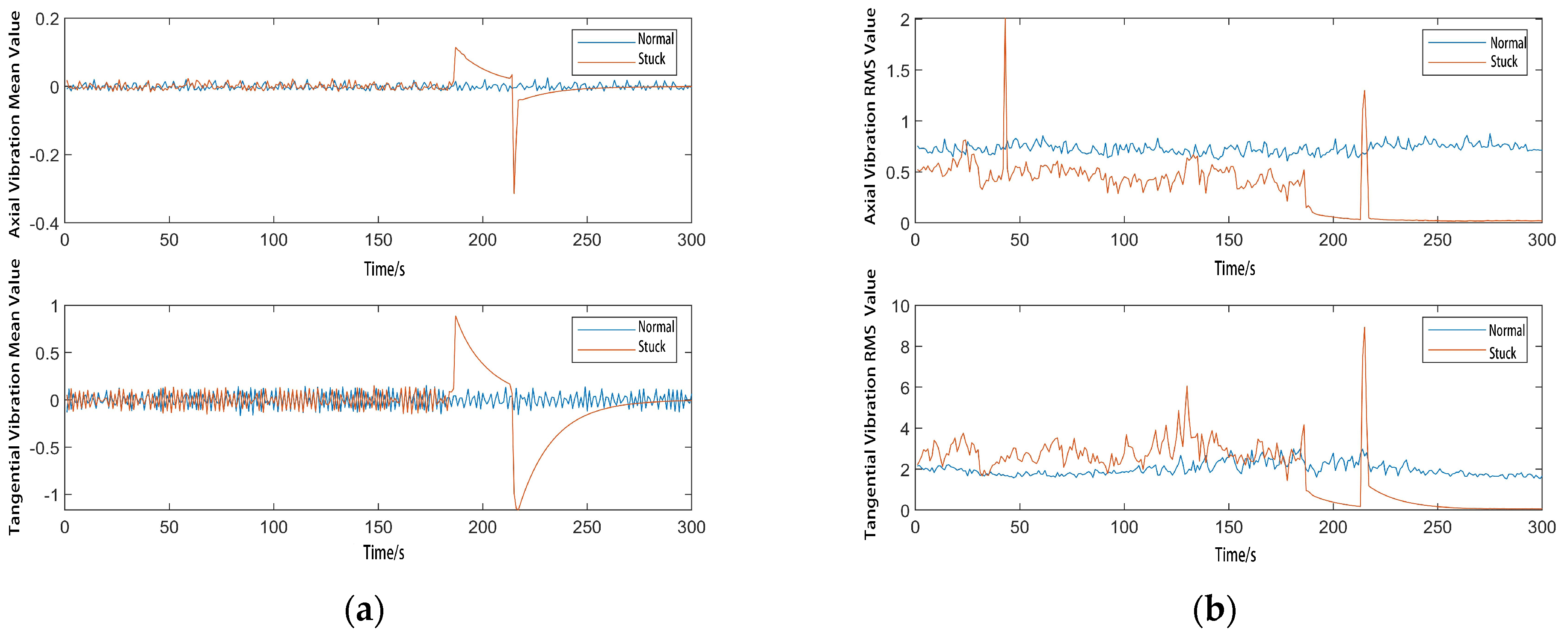
As shown in Figure 4, time domain analysis and processing are conducted on the signals, including probability density function, mean square value, mean value, variance, and correlation analysis, among others. Variance reflects the fluctuation amplitude of the vibration signal, while the mean square value, which is the mean of the squared vibration signal, indicates the average power of the signal. During normal drilling, the mean value of tangential vibration fluctuates around 0, with the root mean square (RMS) value fluctuating around 2 m/s2; the mean value of axial vibration fluctuates around 0, with the RMS value fluctuating around 0.25 m/s2. These characteristics indicate stable drilling. Before a stuck pipe event occurs, the mean and RMS values of tangential vibration are similar to those of normal vibration. The moment a stuck pipe event occurs, the mean values of tangential and axial vibrations undergo violent fluctuations, and the RMS values rapidly increase to around 8 m/s2 after the stuck pipe event.
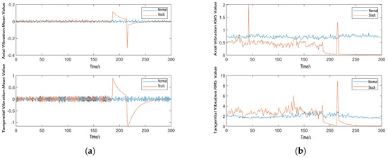
Figure 4.
Vibration analysis of near-bit Data. (a) Axial Vibration Mean Value and Tangential Vibration Mean Value; (b) Axial Vibration RMS Value and Tangential Vibration RMS Value.
3.4. Time-Frequency Domain Analysis
The Short-Time Fourier Transform (STFT) involves segmenting the signal, applying a window function, and then performing the Fast Fourier Transform (FFT) within each window. Before a stuck pipe event occurs, the time-frequency domain shows no significant difference from normal drilling conditions, with the main frequencies concentrated below 200 Hz. As shown in Figure 5, the time-frequency plot reveals that after a stuck pipe event occurs, there is no vibration, and thus no vibration frequency. Therefore, it is not possible to predict a stuck pipe event based on frequency analysis.
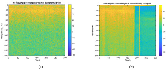
Figure 5.
Time-frequency domain analysis of near-bit data. (a) Time-frequency plot of tangential vibration during normal drilling; (b) Time-frequency plot of tangential vibration during stuck pipe.
By comparing the changes in parameters under normal drilling and stuck pipe conditions in the time domain, frequency domain, time-frequency domain, and vibration, it is found that the parameter characteristics before a stuck pipe event are similar to those during normal drilling. Therefore, it is not possible to extract features before and after a stuck pipe event, making it impossible to predict a stuck pipe occurrence.
4. Experimentation and Analysis
4.1. Data Preprocessing
4.1.1. Parameter Selection
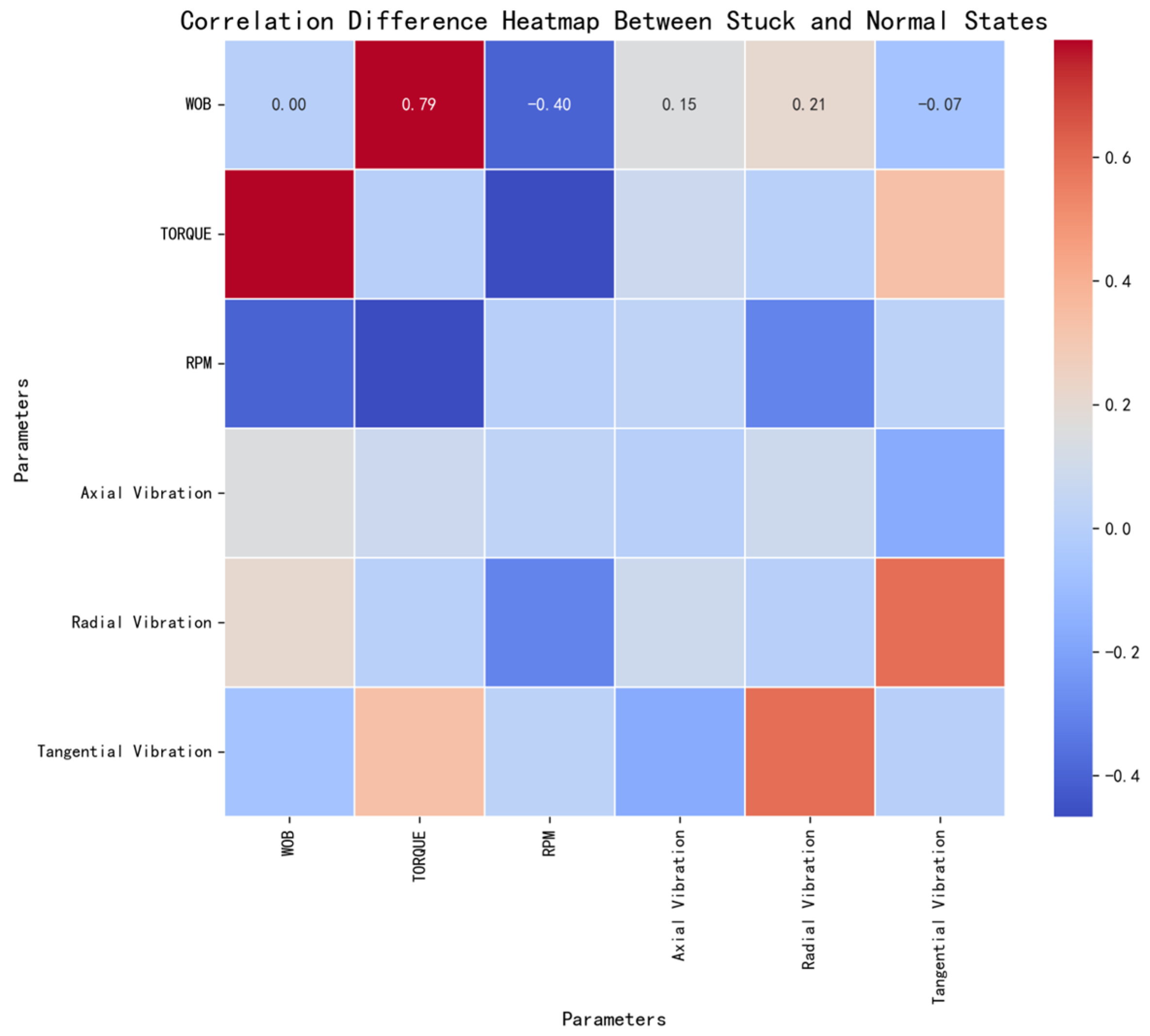
The correlation matrix was calculated separately for the stuck pipe and normal drilling conditions to determine the correlation coefficients between each pair of parameters. The difference in correlation matrices between the two conditions was then computed. As shown in Figure 6, the heatmap reveals significant differences in the correlations between parameters under the two conditions. The correlation difference between drilling pressure and torque is particularly large, with a notable positive correlation (red area, 0.79) in the heatmap. This indicates that the association between drilling pressure and torque is stronger during a stuck pipe event. The correlation between rotational speed and drilling pressure is negative (−0.40), suggesting that during a stuck pipe event, the trend of rotational speed is inversely related to that of drilling pressure. This may reflect that an increase in drilling pressure leads to a decrease in rotational speed during a stuck pipe event. The correlations between axial and normal vibrations show smaller changes, indicated by lighter colors in the heatmap. This suggests that the relationship between these two parameters remains relatively stable and is not significantly affected by the stuck pipe condition.

Figure 6.
Heatmap of differences in correlation of drilling parameters between sticking and normal drilling conditions.
4.1.2. Mode Decomposition Techniques
- Empirical Mode Decomposition (EMD)
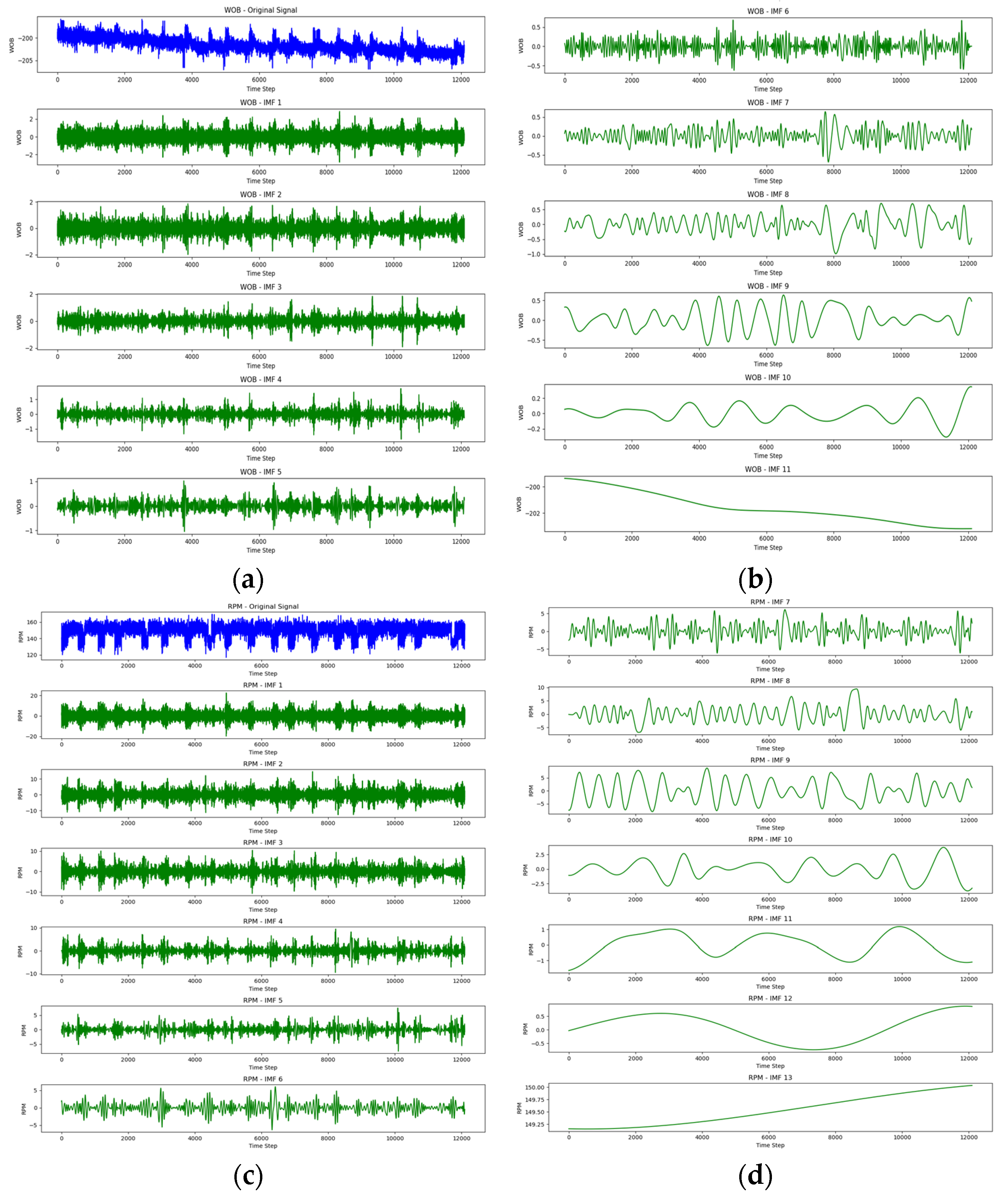
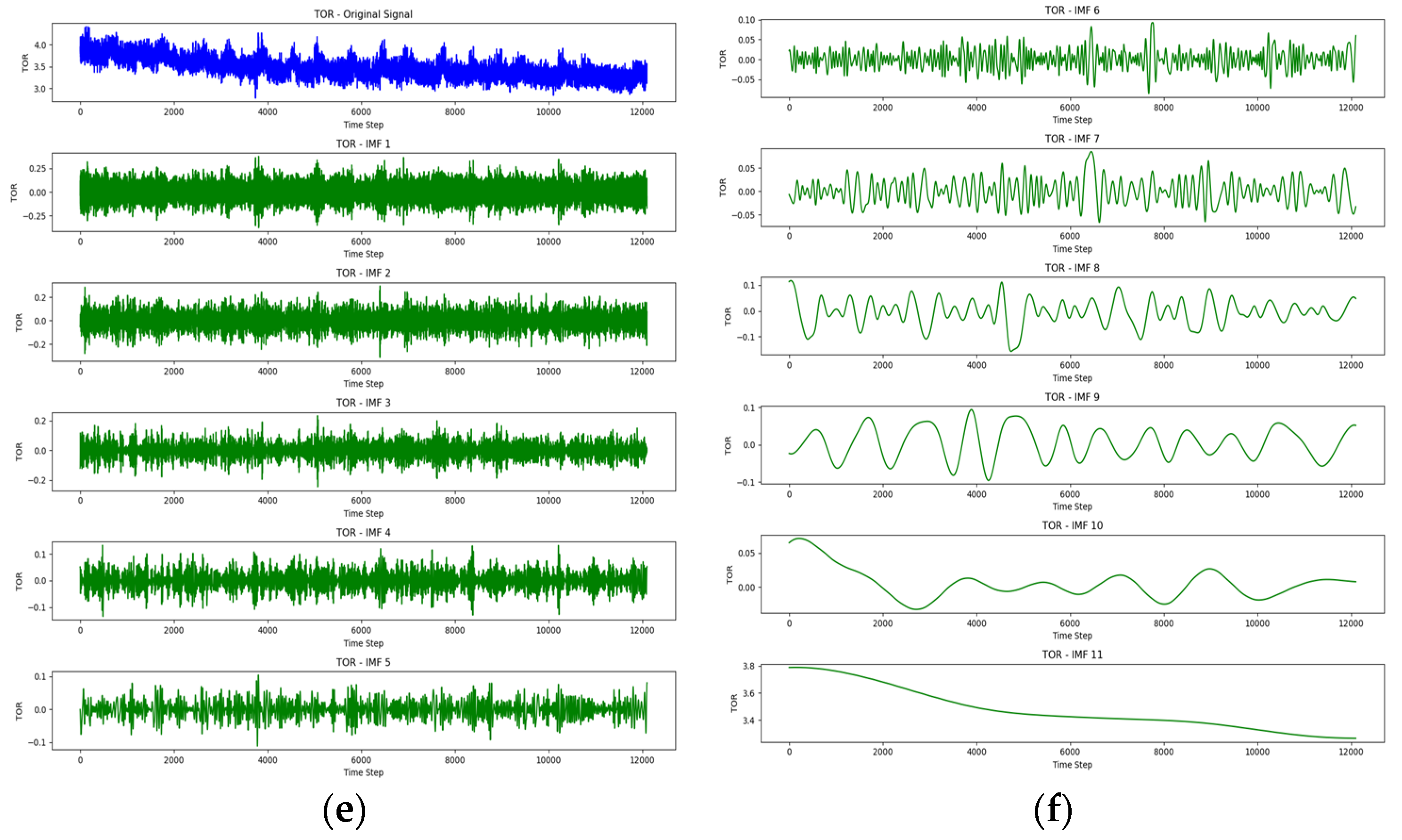
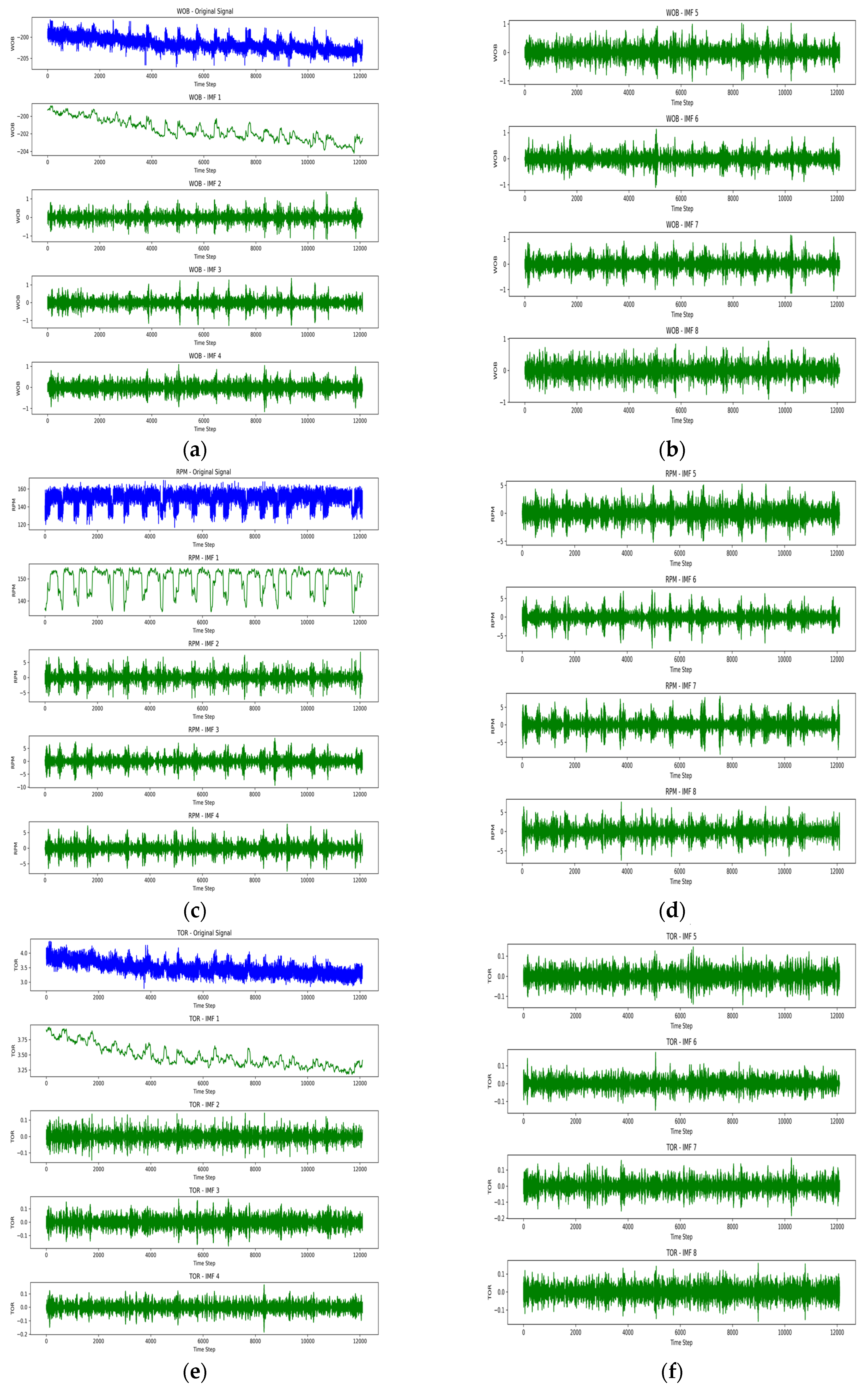
Empirical Mode Decomposition (EMD) is a data-driven and adaptive time-series analysis technique designed to decompose nonlinear and non-stationary signals into a finite set of oscillatory components known as Intrinsic Mode Functions (IMFs). In this study, EMD is first applied to the input signals, including WOB, TOR, and RPM, to obtain a series of IMFs, as illustrated in Figure 7. To evaluate the relevance of each decomposed component, the Pearson correlation coefficients between each IMF (obtained by EMD) or each mode (obtained by VMD) and the original target variables (WOB, TOR, and RPM) were calculated. Table 2 presents the correlation results, where higher absolute values indicate stronger relevance between the decomposed components and the original signals. The most relevant components were selected based on these correlations and subsequently recombined to form the reconstructed signals used for forecasting.
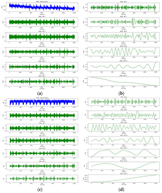

Figure 7.
IMFs of WOB, TOR, and RPM signals after EMD. (a,b) IMFs of WOB signals after EMD; (c,d) IMFs of TOR signals after EMD; (e,f) IMFs of RPM signals after EMD.
Table 2.
IMF correlations of WOB, TOR, and RPM signals.
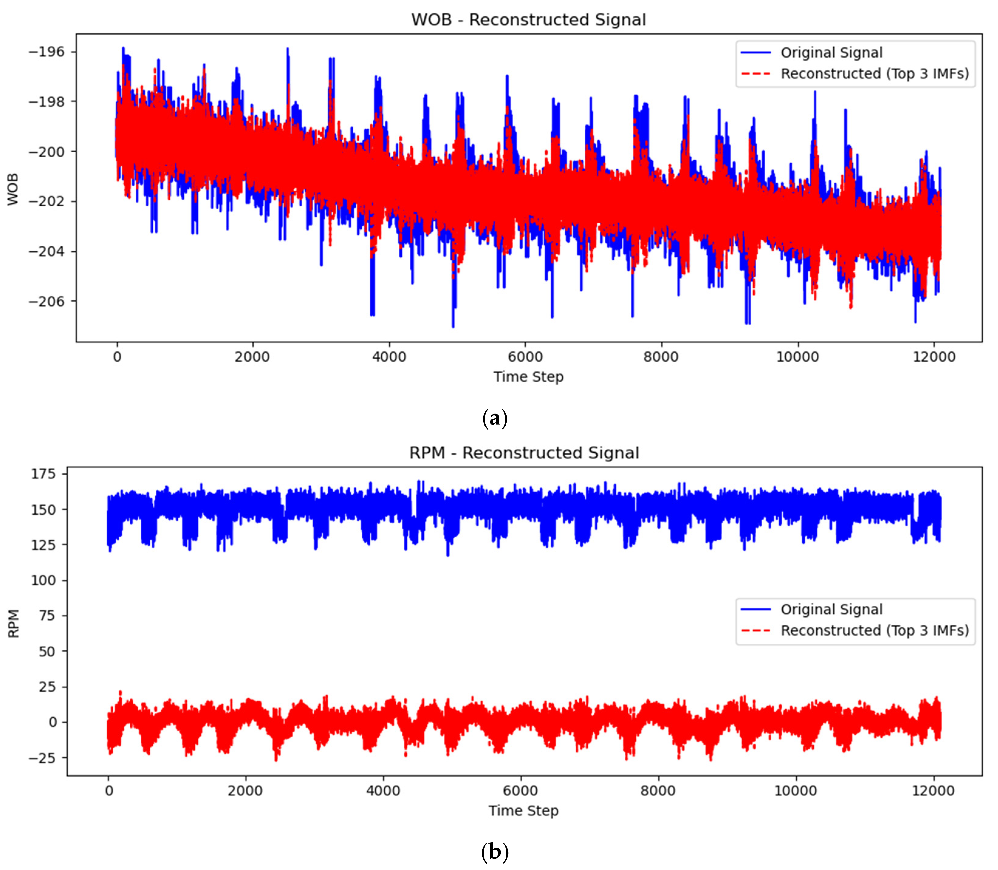
As shown in Figure 8, from the comparison of the reconstructed signal and the original signal during normal drilling, the following observations can be made:


Figure 8.
Reconstructed WOB, TOR, and RPM signals after EMD. (a) Comparison Between WOB Original Signal and Reconstructed Signal; (b) Comparison Between RPM Original Signal and Reconstructed Signal; (c) Comparison Between TOR Original Signal and Reconstructed Signal.
WOB (Weight on Bit): The original signal (blue line) contains a lot of high-frequency noise and fluctuations, while the reconstructed signal (red line) shows a much smoother trend. This smoothness removes instantaneous disturbances and retains the long-term trend of the signal, especially during the phase when the WOB is gradually decreasing. By observing the reconstructed signal, a continuous decline in WOB is evident, and the fluctuations become more stable. This could be a precursor to a stuck pipe event, as the WOB typically increases gradually or changes at a slower rate before such an event occurs.
TOR (Torque): Similar to WOB, the high-frequency fluctuations in the original signal are smoothed out in the reconstructed signal. Although the changes in torque are relatively small, the reconstructed signal shows a clearer trend compared to the original signal, which is very helpful for monitoring potential stuck pipe events. The stability of the torque could reflect subtle changes in the tool before encountering a stuck condition.
RPM (Rotations Per Minute): The original signal shows severe fluctuations, while the reconstructed signal suppresses irrelevant high-frequency noise and highlights the periodic fluctuations in RPM. Before a stuck pipe event, the RPM fluctuations might become more regular, and the reconstructed signal can better reveal this change, helping to detect potential anomalies.
The precursor to a stuck pipe event is typically a gradual change rather than an abrupt one. The smoothness of the reconstructed signal allows us to observe gradual changes that were masked by noise in the original signal. Particularly in the reconstructed signals for WOB and TOR, the trend changes (such as a gradual decrease in WOB or a steady increase in TOR) could serve as early warning signals before a stuck pipe event occurs. By selecting the IMF components with high correlation, the reconstructed signal eliminates irrelevant high-frequency noise, which is crucial for understanding the fundamental trend of the signal. Before a stuck pipe event, the original signal may contain many transient high-frequency fluctuations, which are not directly meaningful. However, the reconstructed signal can remove these fluctuations, revealing the long-term changes associated with the stuck pipe event. The WOB-reconstructed signal is clearly much smoother and the trend is more distinct compared to the original signal, with larger and more stable changes in WOB before the stuck pipe event, which suggests that the reconstructed signal better captures the gradual increase in WOB. The RPM-reconstructed signal shows a more evident regularity and fluctuation, appearing much more stable compared to the chaotic fluctuations in the original signal, which can help us capture potential changes before the stuck pipe event. The TOR-reconstructed signal also shows smooth variation after noise removal. Compared to the high-frequency fluctuations in the original signal, many irrelevant changes are removed, aiding in a clearer analysis of the slow-changing trend before the stuck pipe event.
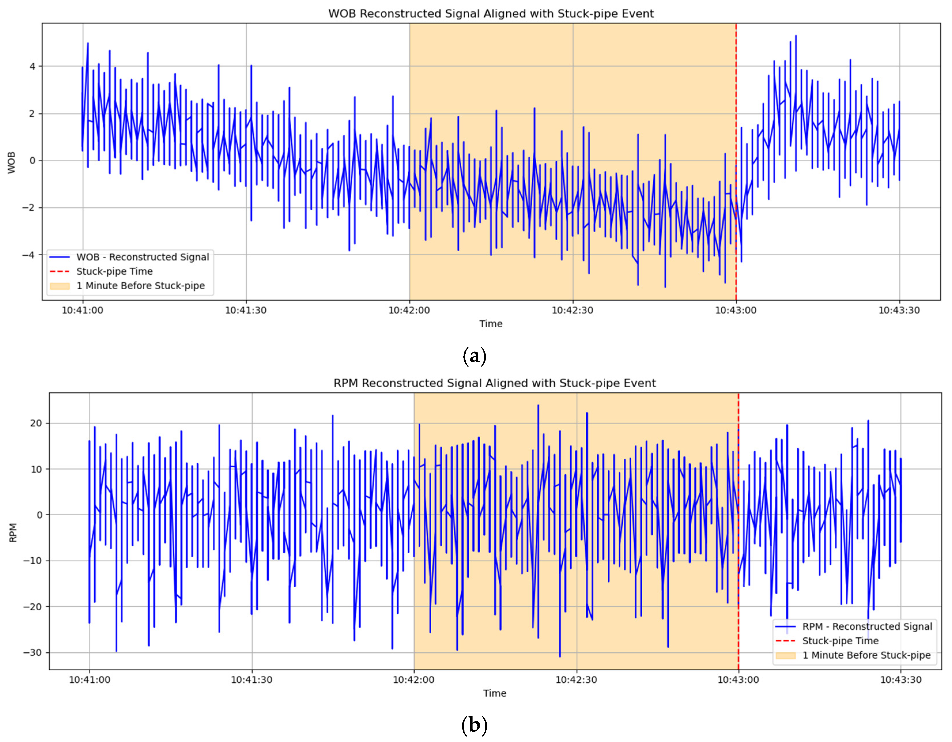
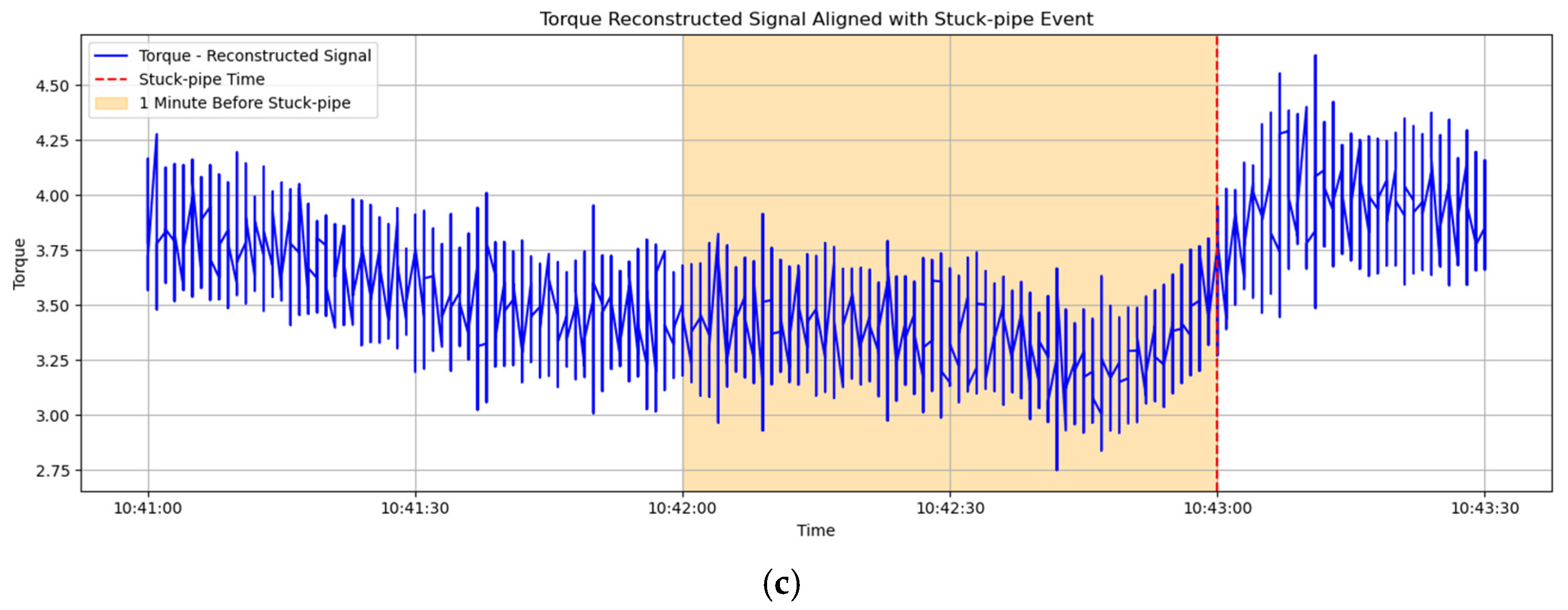
As shown in Figure 9, by observing the reconstructed signals during normal drilling and after the occurrence of a stuck pipe event, it can be seen that the WOB (Weight on Bit) value decreases and the fluctuations decrease before the stuck pipe event. This may be due to the drilling tool being stuck, increasing friction. Before the stuck pipe event, the fluctuation in torque gradually decreases, possibly reflecting changes in mechanical resistance. This is difficult to detect in the original signal, but it can be clearly seen in the reconstructed signal. The reconstructed signal may show periodic changes in RPM (Rotations Per Minute). Before the stuck pipe event, due to the effect of the stuck condition, the RPM cycle might become more regular or show increased changes.


Figure 9.
Extract meaningful features from the reconstructed signals during normal drilling. (a) WOB Reconstructed Signal Aligned with Stuck-pipe Event; (b) RPM Reconstructed Signal Aligned with Stuck-pipe Event; (c) TOR Reconstructed Signal Aligned with Stuck-pipe Event.
- 2.
- Variational Mode Decomposition (VMD)
Variational Mode Decomposition (VMD) is a recently developed signal processing technique based on variational principles, which decomposes complex signals into a set of band-limited intrinsic mode components with well-defined center frequencies. Unlike EMD, VMD formulates the decomposition process as a constrained variational optimization problem, wherein each mode is obtained by minimizing its spectral bandwidth. The decomposition is governed by two key parameters: the number of modes K and the penalty factor α. As shown in Figure 10, VMD is utilized to decompose the original signals into multiple modes. Subsequently, as shown in Table 3, the Pearson correlation coefficients between each mode and the original signal are computed and recombined to reconstruct a new signal.
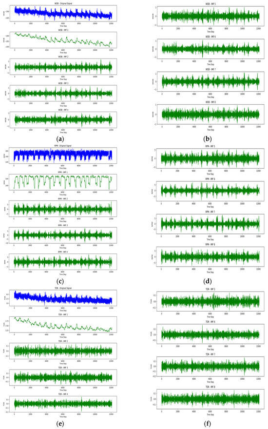
Figure 10.
IMFs of WOB, torque, and RPM signals after VMD. (a,b) IMFs of WOB signals after VMD; (c,d) IMFs of TOR signals after VMD; (e,f) IMFs of RPM signals after VMD.
Table 3.
IMF correlations of the three signals.
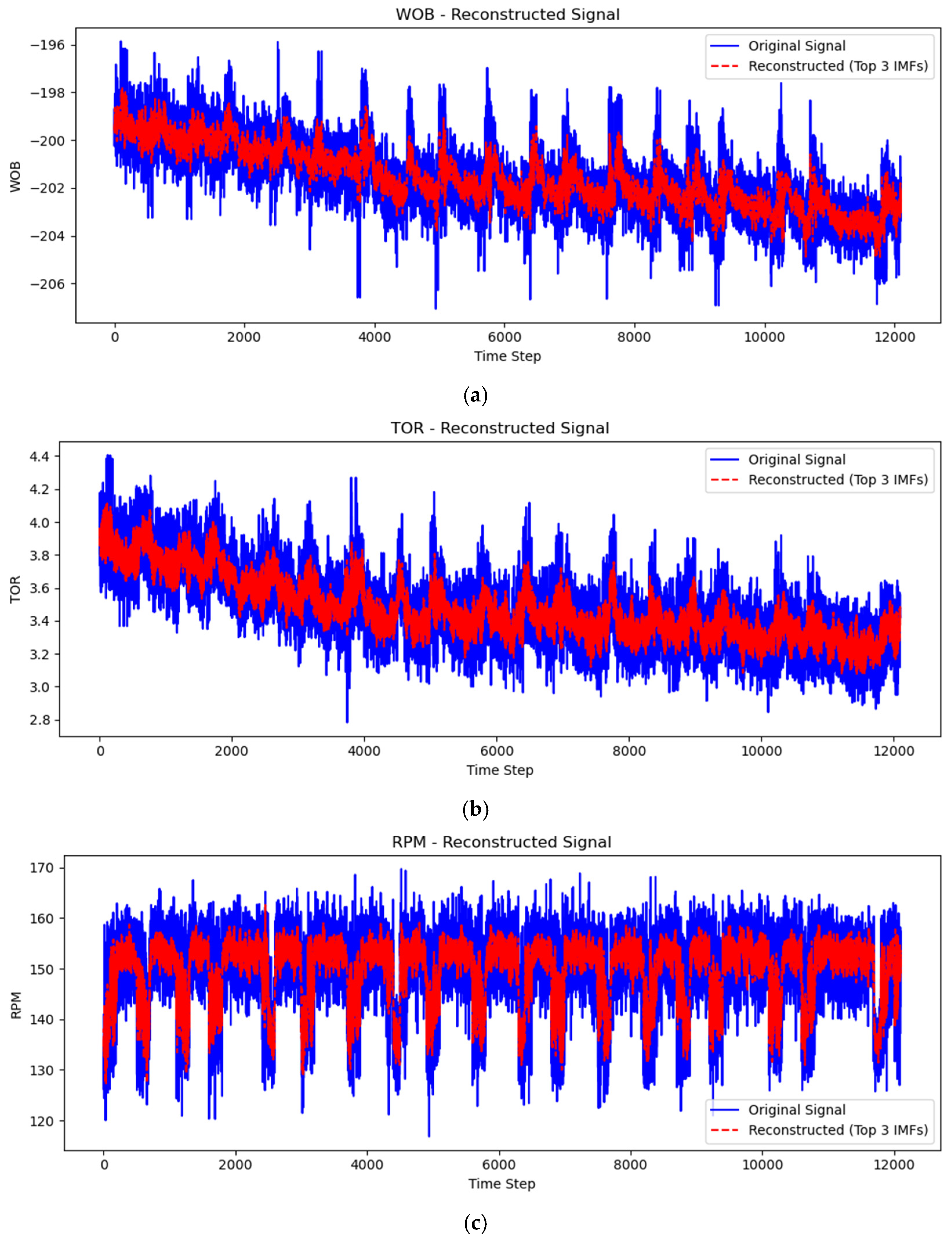
As shown in Figure 11, VMD has a stronger capability to handle non-stationary and noisy signals by adapting its frequency decomposition based on the data. This results in better separation of signal components, especially when the signal is highly fluctuating or has overlapping frequency components. VMD focuses on extracting modes with less noise and provides a more stable frequency separation, which helps in revealing trends that might not be visible in the EMD due to its sensitivity to high-frequency noise.

Figure 11.
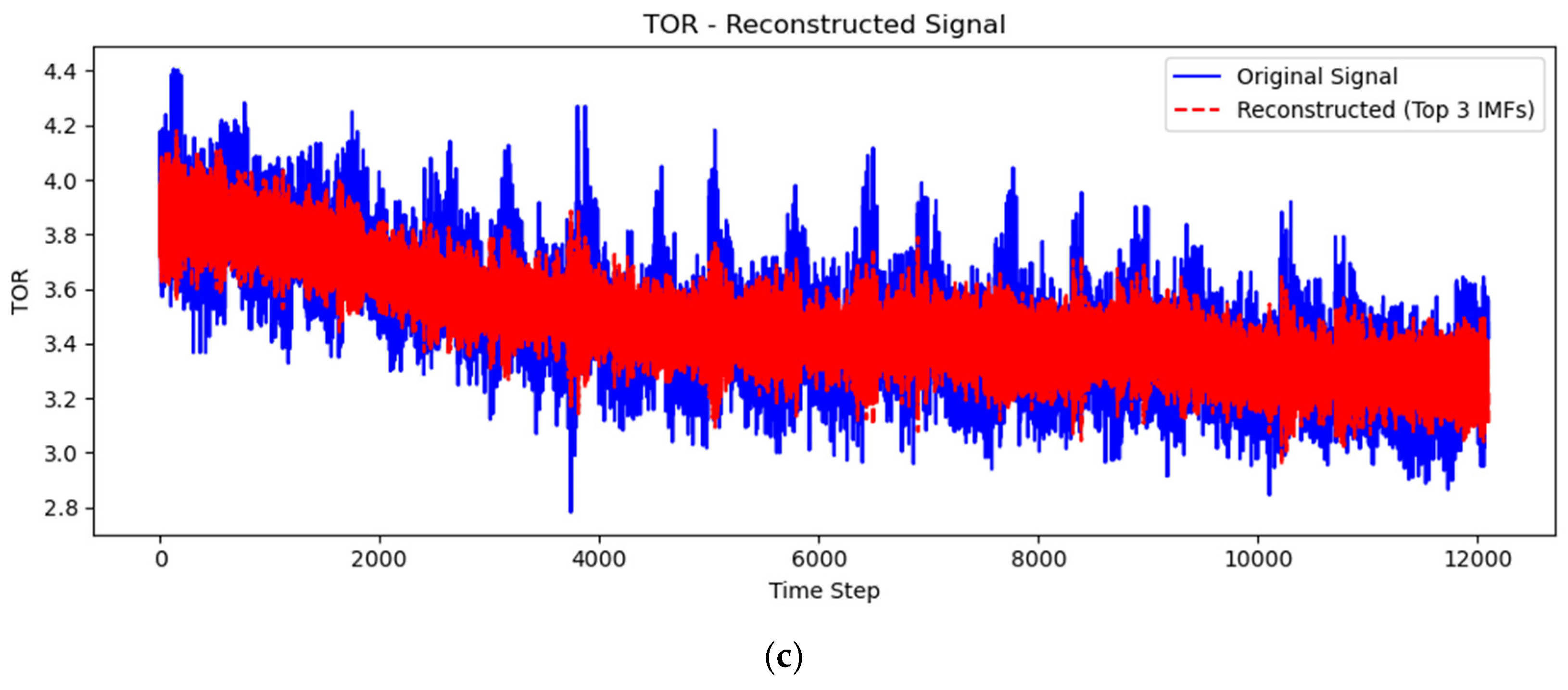
Reconstructed WOB, TOR, and RPM signals after VMD. (a) Comparison Between WOB Original Signal and Reconstructed Signal; (b) Comparison Between TOR Original Signal and Reconstructed Signal; (c) Comparison Between RPM Original Signal and Reconstructed Signal.
WOB (Weight on Bit): The original WOB signal is highly fluctuating with a lot of high-frequency noise, making it difficult to observe long-term trends or gradual changes leading up to the stuck pipe event. In contrast, the reconstructed signal after VMD processing is smoother, and the gradual decline in WOB is more visible. This decline in WOB, with less fluctuation, is indicative of increased resistance or friction—a potential sign of the tool becoming stuck. The gradual decrease in WOB (more apparent in the reconstructed signal) suggests that the drilling tool is experiencing increasing friction, which is a key precursor to a stuck pipe event.
TOR (Torque): The original torque signal shows significant noise and rapid fluctuations, making it difficult to discern clear trends or shifts in mechanical resistance before a stuck pipe event. VMD helps to smooth out the high-frequency fluctuations and highlights the trend in torque. Even if torque changes are smaller in magnitude, the trend is clearer, which is critical for detecting subtle mechanical issues that can precede a stuck pipe event. The reduction in torque fluctuations or a more stable pattern in the reconstructed signal reflects increased mechanical resistance as the tool approaches a stuck condition.
RPM (Rotations Per Minute): The original RPM signal is full of high-frequency fluctuations, making it difficult to interpret. After VMD processing, the reconstructed RPM signal shows more periodicity and smoother transitions. Before a stuck pipe event, RPM often exhibits more regular cycles or a higher-amplitude pattern, which can indicate that the system is under stress. The reconstructed RPM signal reveals periodic changes or more regular cycles, which may signal increased friction or a gradual mechanical change leading up to the stuck pipe event.
As shown in Figure 12, by observing the reconstructed signals during normal drilling and after the occurrence of a stuck pipe event, the gradual decrease in Weight on Bit and the reduction in fluctuations may be due to the drilling tools becoming stuck, resulting in increased friction. The reduction in torque fluctuations may reflect changes in mechanical resistance. The periodic changes in rotational speed may be another signal of impending sticking.
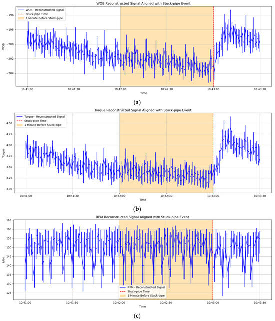
Figure 12.
Extracted meaningful features from the reconstructed signals during normal drilling.
4.2. Model Construction
4.2.1. Rationale for a Data-Physics Dual-Driven Approach
In the context of stuck pipe prediction, data imbalance—where normal drilling data vastly exceeds instances of a stuck pipe—presents a significant challenge for purely data-driven models. As illustrated in Figure 13, traditional physics-based models depend on well-established physical laws and retain certain predictive capabilities under limited data conditions. However, their adaptability to complex, dynamic field environments is often constrained. Conversely, data-driven models rely heavily on large volumes of historical data. While they can achieve high accuracy under abundant data conditions, their performance deteriorates in rare-event scenarios due to overfitting and a lack of physical interpretability.

Figure 13.
Three modeling approaches.
The Data-Physics dual-driven approach offers a promising solution by integrating partial physical knowledge with available data. As shown in the overlapping region of partial data and partial physics in the figure, this hybrid framework leverages the strengths of both paradigms: it enhances model generalization in data-scarce conditions and improves interpretability through embedded physical constraints. This makes it particularly effective in high-risk drilling operations characterized by data imbalance and partial domain knowledge.
These findings collectively underscore the advantages of the Data-Physics dual-driven paradigm in addressing data imbalance, enhancing robustness, and improving interpretability in stuck pipe prediction tasks.
4.2.2. CNN-LSTM-Attention Architecture
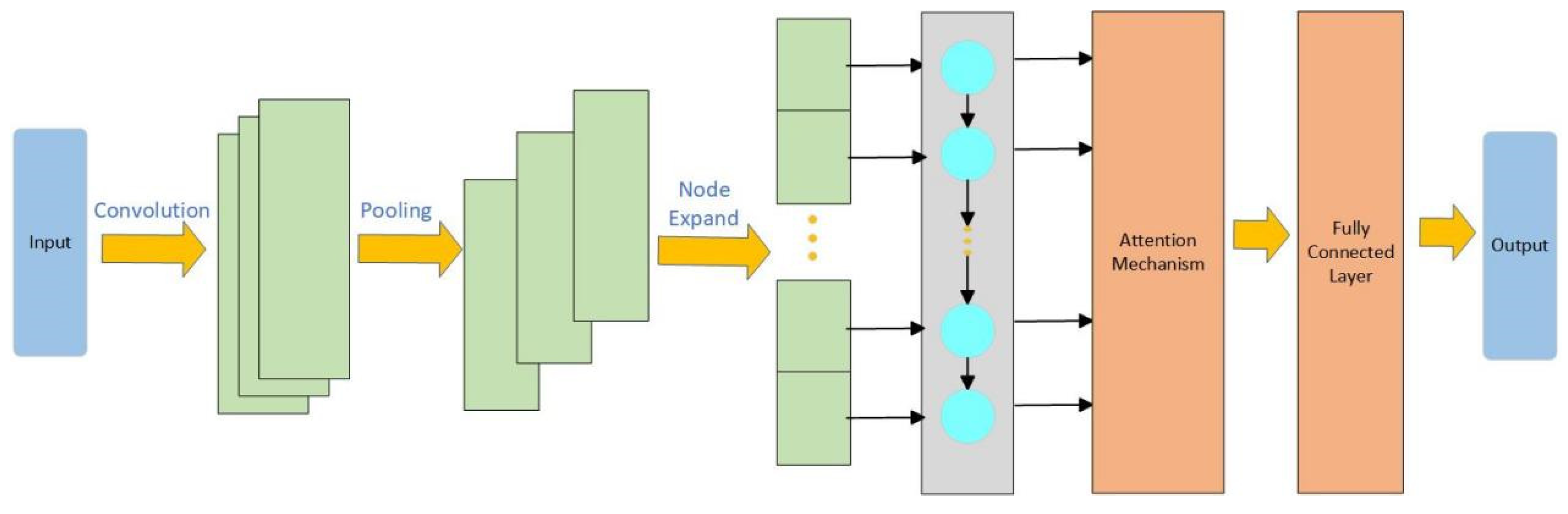
The CNN-LSTM-Attention [27] architecture is shown in Figure 14, which includes the input layer, convolutional layer, pooling layer, LSTM layer, Attention layer, and fully connected layer.

Figure 14.
CNN-LSTM-Attention architecture.
Input Layer: The input is the new signal obtained after modal decomposition.
Convolutional Layer: This layer is used to extract local temporal features from the input data. Through convolution operations, it can process the data locally at each time step and identify local patterns.
Pooling Layer: The pooling layer reduces the dimensionality of the features through down sampling, decreases the computational load, and enhances the model’s robustness to local features.
LSTM Layer [28]: The LSTM layer is used to capture long-term dependencies in time-series data. Through its memory cells, LSTM can effectively retain historical information and utilize it in the computation of the current time step.
Attention Layer: This layer optimizes the model’s focus on important time steps. The Attention mechanism helps the model concentrate on significant parts of the input sequence. By calculating the importance weights for each time step, the model can selectively focus on key time steps, thereby improving the prediction accuracy. In this model, the Attention mechanism is applied to the output of the LSTM layer to enhance the model’s focus on important time steps.
Fully Connected Layer: The final output from the LSTM layer is passed to the fully connected layer for the final prediction.
In this study, the forecasting task is formulated as a one-step-ahead prediction problem. The model inputs a sequence consisting of the past 50 time steps of three drilling parameters (Weight on Bit, torque, and rotary speed), and predicts the corresponding values of these parameters at the next time step.
In this study, the primary forecasting task is formulated as a one-step-ahead prediction, where the model takes the past 50 time steps of three key drilling parameters—Weight on Bit (WOB), torque (TOR), and rotary speed (RPM)—as input, and predicts their values at the next time step. The input is represented as a three-dimensional tensor with shape (samples, 50, 3), and the output is a two-dimensional array of shape (samples, 3) for simultaneous prediction of all three parameters.
To further evaluate the model’s potential for real-world early warning applications, we additionally conducted a single set of multi-step prediction experiments, extending the forecast horizon to three steps (approximately 15 s). In this case, the model output takes the shape (samples, 3, 3), representing predicted values of all three parameters over the next three time steps.
4.2.3. Design of Adaptive Physics-Constrained Loss Function
- Gradient Constraint
Gradient constraints are commonly used to ensure that the rate of change of a signal or physical quantity is consistent with actual physical phenomena. In many physical systems, the changes in signals are regular, especially in dynamic systems where the gradients (i.e., rates of change) between signals [29] follow certain physical laws. The purpose of the gradient constraint is to make the gradient relationship between drilling pressure and rotational speed (driven by torque) more consistent with physical laws. The formula for the gradient constraint is as follows:
The assumption of the physical constraint is that the product of the two gradients should be close to 1 or some other constant value (depending on the specific physical context). Therefore, the loss function includes this term:
- 2.
- Power Constraint
The assumption of the physical constraint is that the product of the two gradients should be close to 1 or some other constant [30] value (depending on the specific physical context). Therefore, the loss function includes this term:
The power error is incorporated into the loss function, as shown in Equation (13):
- 3.
- Design of Adaptive Weights
The adjustment of weights depends on the error in each constraint part of the model [31]. Specifically, as shown in Equations (14) and (15):
In Equations (14) and (15):
and are the initial weight, with an initial value set to 0.2.
represents the average of the drilling pressure prediction error. The larger the error, the greater the weight, indicating that the influence of the physical constraint on drilling pressure will be enhanced. Similarly, is used to adjust the weight for torque.
- 4.
- Design of the Final Loss Function
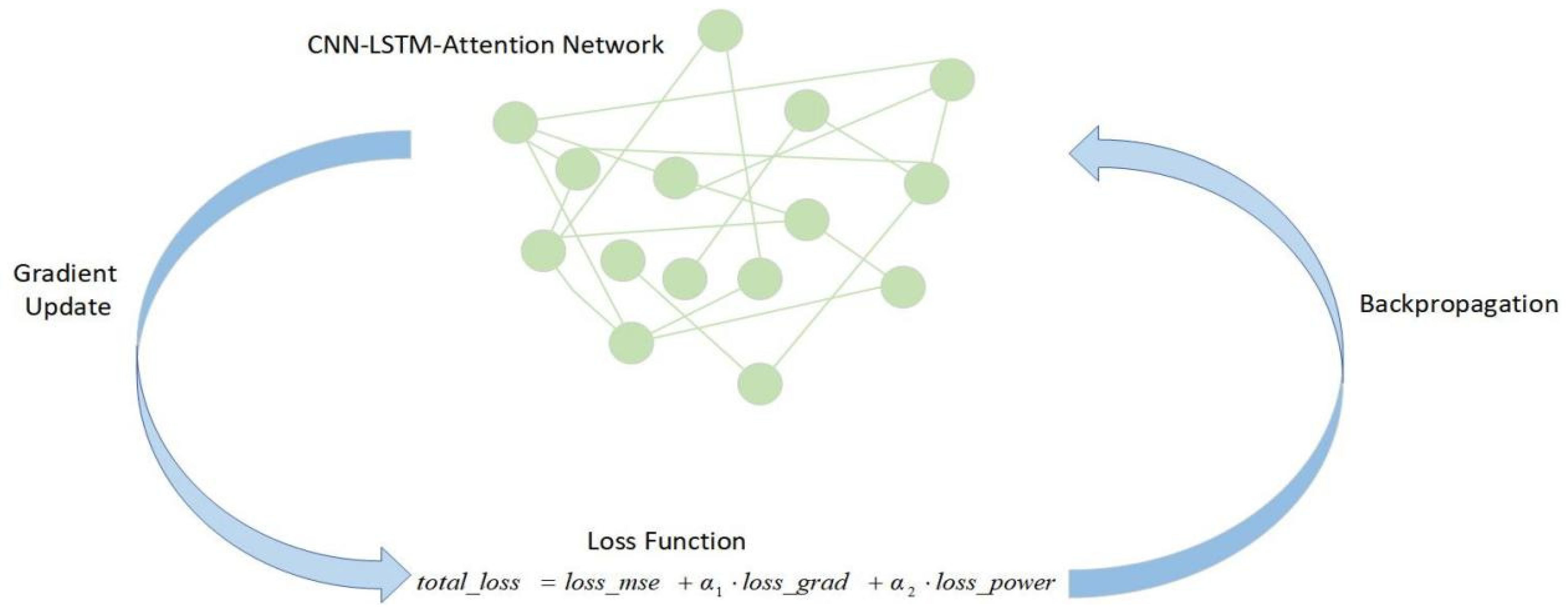
As shown in Figure 15, by integrating the main loss (MSE) and the loss from the physical constraints, the final loss function is obtained, as shown in Equation (16):
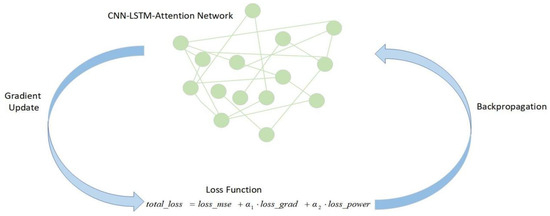
Figure 15.
The relationship between loss function and network.
In this Equation:
: Main loss, measuring the error between the predicted and true values.
: Gradient constraint loss, ensuring that the relationship between drilling pressure and rotational speed conforms to physical laws.
: Power constraint loss, ensuring that the product of torque and rotational speed (i.e., power) conforms to physical laws.
, : The weight dynamically adjusted based on the error.
4.3. Model Construction
4.3.1. The Role of Physical Constraints in the Model
Table 4 presents the evaluation metrics for the models, including running time MSE, MAE, and R2, which are used to assess the accuracy of the prediction models. As shown in Table 4, without the introduction of physical constraints, the VMD + CNN-LSTM-Attention model’s prediction results for WOB are MSE: 0.3963, MAE: 0.5306, and R2: 0.5715, indicating a moderate level of fitting capability. However, when physical constraints are introduced, the model’s MSE significantly decreases to 0.1700, MAE drops to 0.3319, and R2 increases to 0.9128.
Table 4.
Model comparison.
For the TOR variable, without physical constraints, the prediction results are MSE: 0.0138, MAE: 0.0944, and R2: 0.5926, suggesting that the model has a moderate predictive capability for this variable. However, with the introduction of physical constraints, the MSE significantly drops to 0.0034, MAE decreases to 0.0477, and R2 rises to 0.8993, demonstrating an enhanced ability of the model to capture the dynamic characteristics of torque.
In the prediction of RPM, the model without physical constraints shows MSE: 5.1653, MAE: 1.8672, and R2: 0.8581, which already indicates a relatively high predictive capability. However, after incorporating physical constraints, the MSE significantly reduces to 1.0040, MAE decreases to 0.7626, and R2 markedly increases to 0.9801.
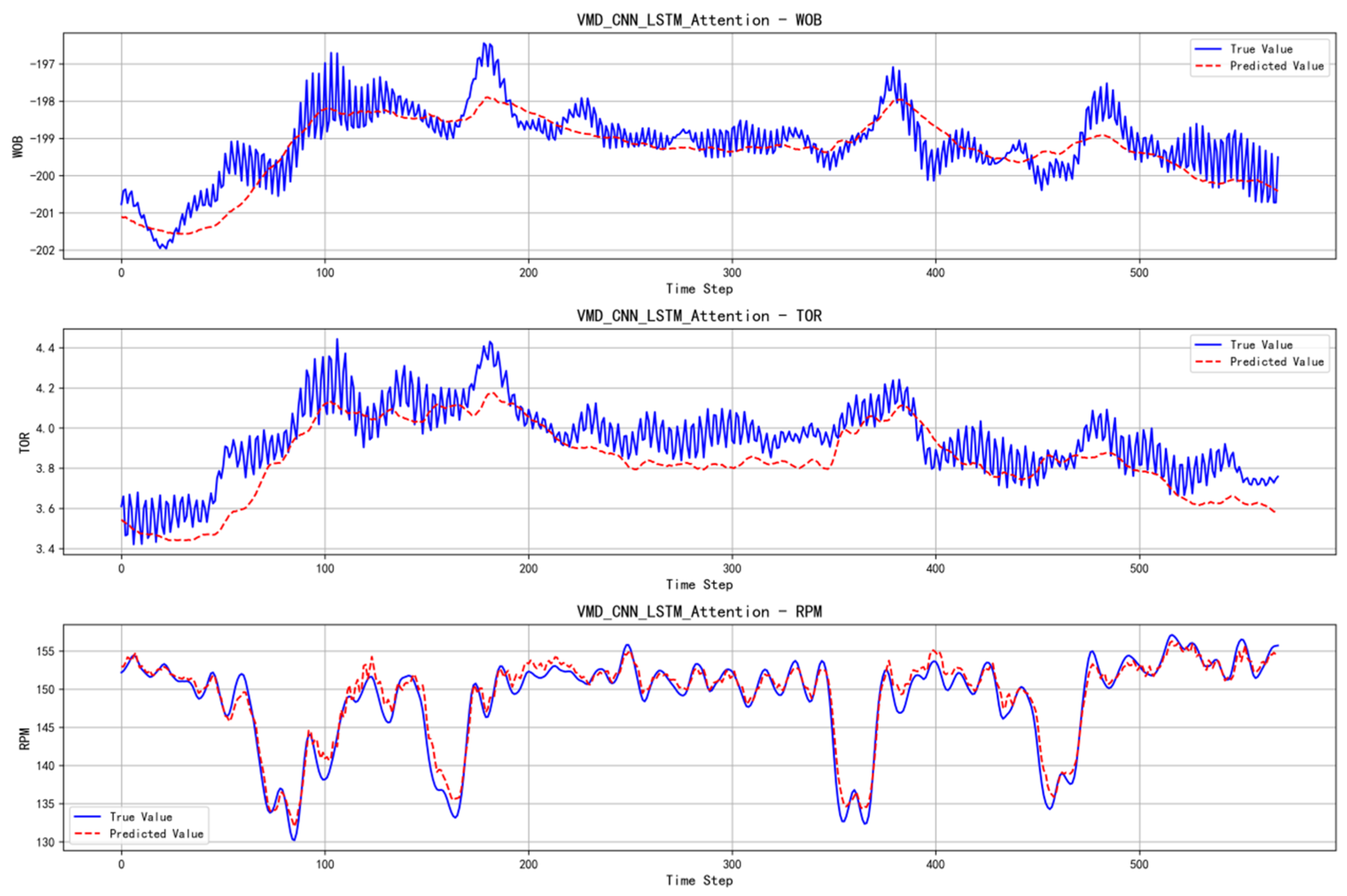
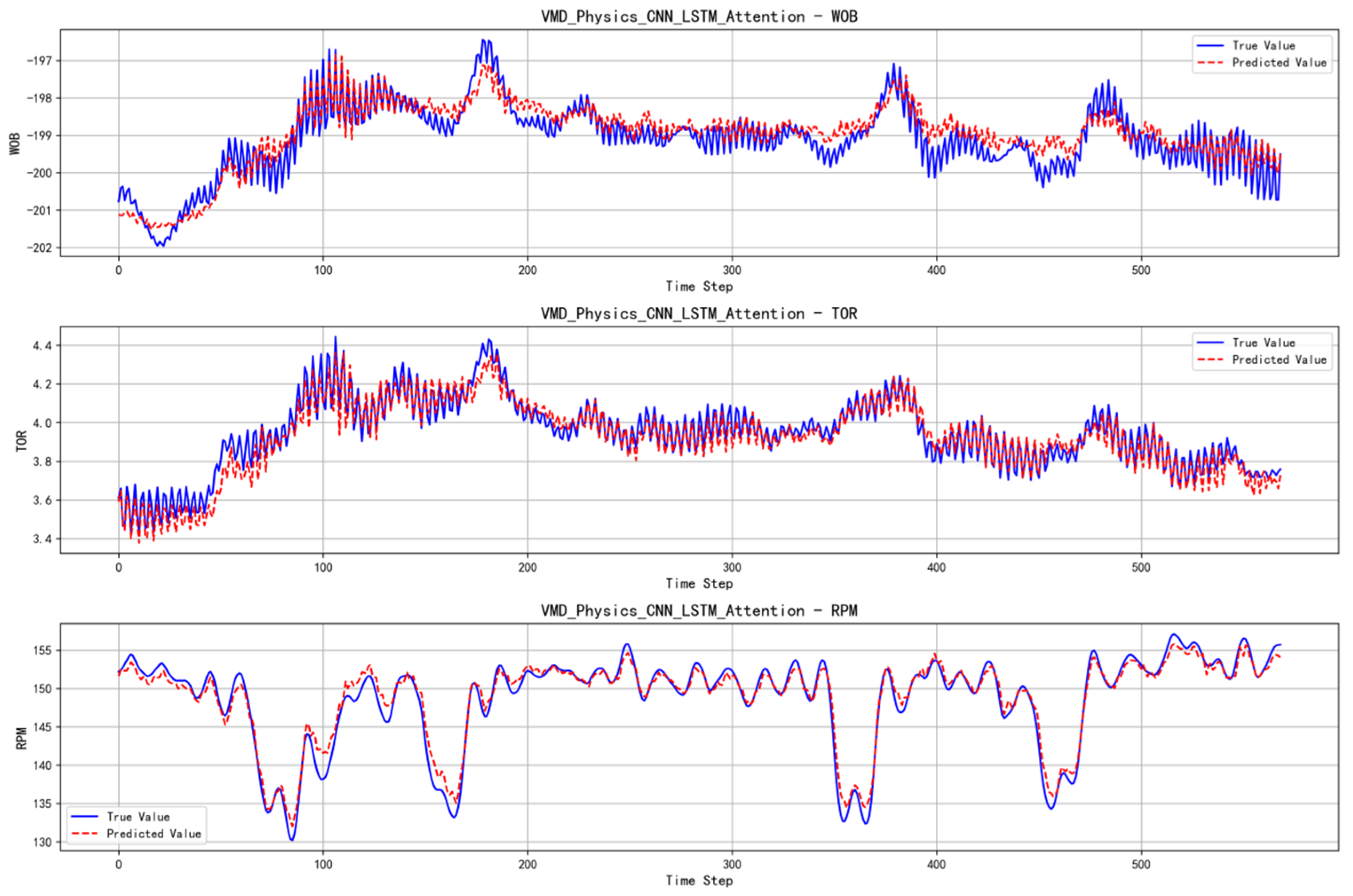
As shown in Figure 16 and Figure 17, the VMD + CNN-LSTM-Attention model exhibits significant deviations in predicting signal peaks without the introduction of physical constraints. In contrast, with the incorporation of physical constraints, the prediction results become much closer to the true values.
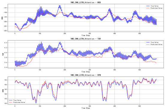
Figure 16.
Prediction performance of a VMD—CNN-LSTM-Attention model.
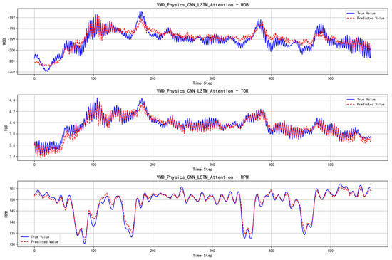
Figure 17.
Prediction performance of a VMD—Physical—CNN-LSTM-Attention model.
In Table 5, for the prediction of WOB, the EMD + CNN-LSTM-Attention model exhibited a relatively high level of error, with an MSE of 1.0888, an MAE of 0.8331, and an R2 of only 0.4131, indicating limited effectiveness in predicting drilling pressure. However, after incorporating physical constraints, the model’s performance in predicting drilling pressure improved significantly, with the MSE decreasing to 0.8935, the MAE reducing to 0.7496, and the R2 increasing to 0.5183. This suggests that the model, enhanced by physical mechanisms, is better able to capture the patterns of change in WOB.
Table 5.
Model comparison.
For TOR prediction, both models performed well, with a slight improvement in predictive performance after the introduction of physical constraints. The EMD + CNN-LSTM-Attention model had an MSE of 0.0089, an MAE of 0.0705, and an R2 of 0.8058, demonstrating high accuracy in torque prediction. The model with the incorporation of physical mechanisms further enhanced its predictive capability, with an MSE of 0.0074, an MAE of 0.0659, and an R2 of 0.8382. This indicates that the introduction of physical mechanisms effectively strengthened the model’s understanding and predictive ability for torque changes.
In terms of RPM prediction, neither model performed satisfactorily, with MSE values of 33.7098 and 25.5727, MAE values of 4.5010 and 4.0667, and low R2 values of 0.0782 and 0.3007, respectively. Although the model incorporating physical mechanisms slightly improved the prediction accuracy of rotational speed, its performance still failed to meet the requirements of practical applications. Rotational speed prediction remains a key area where the model needs further optimization.
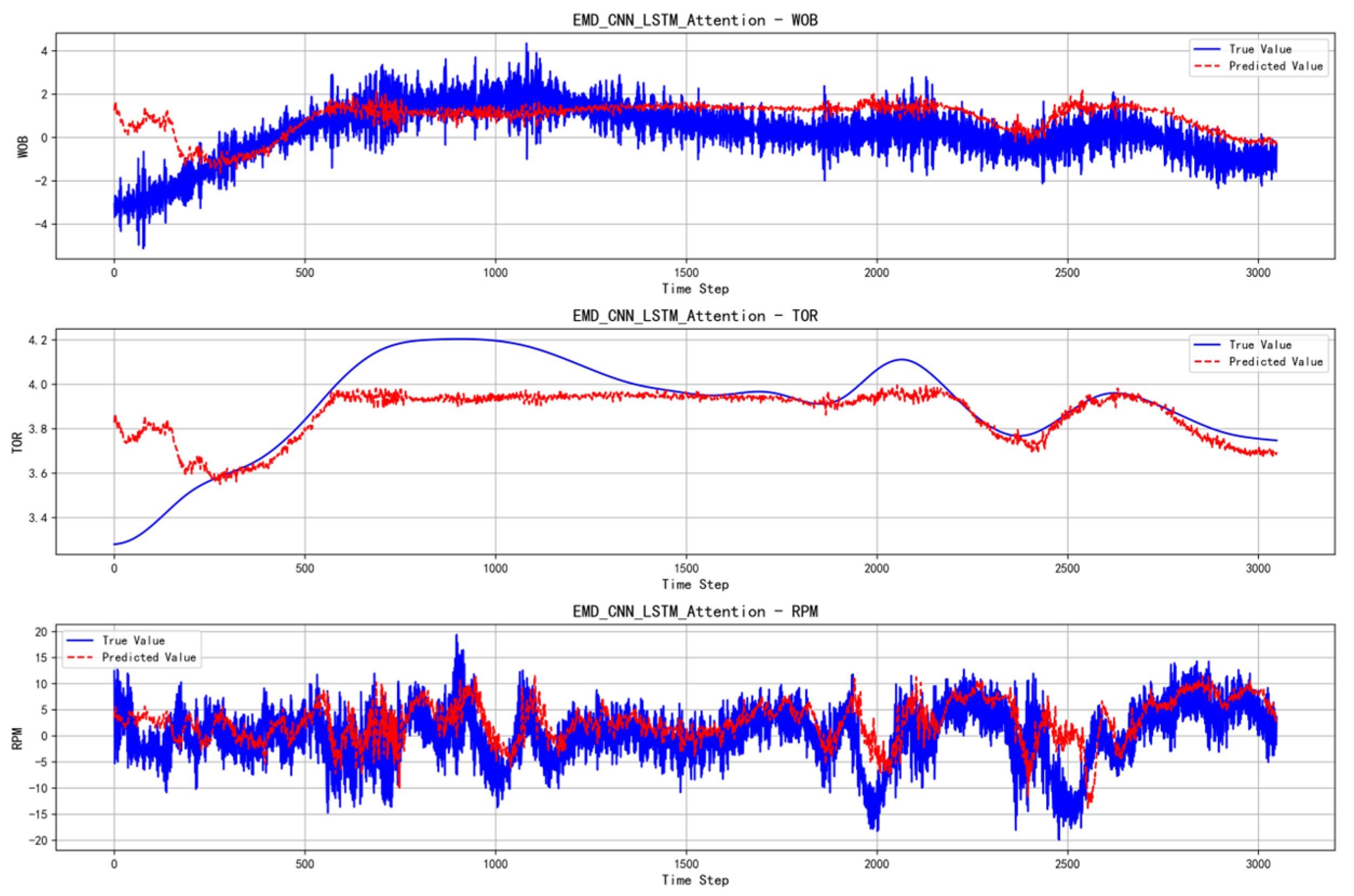
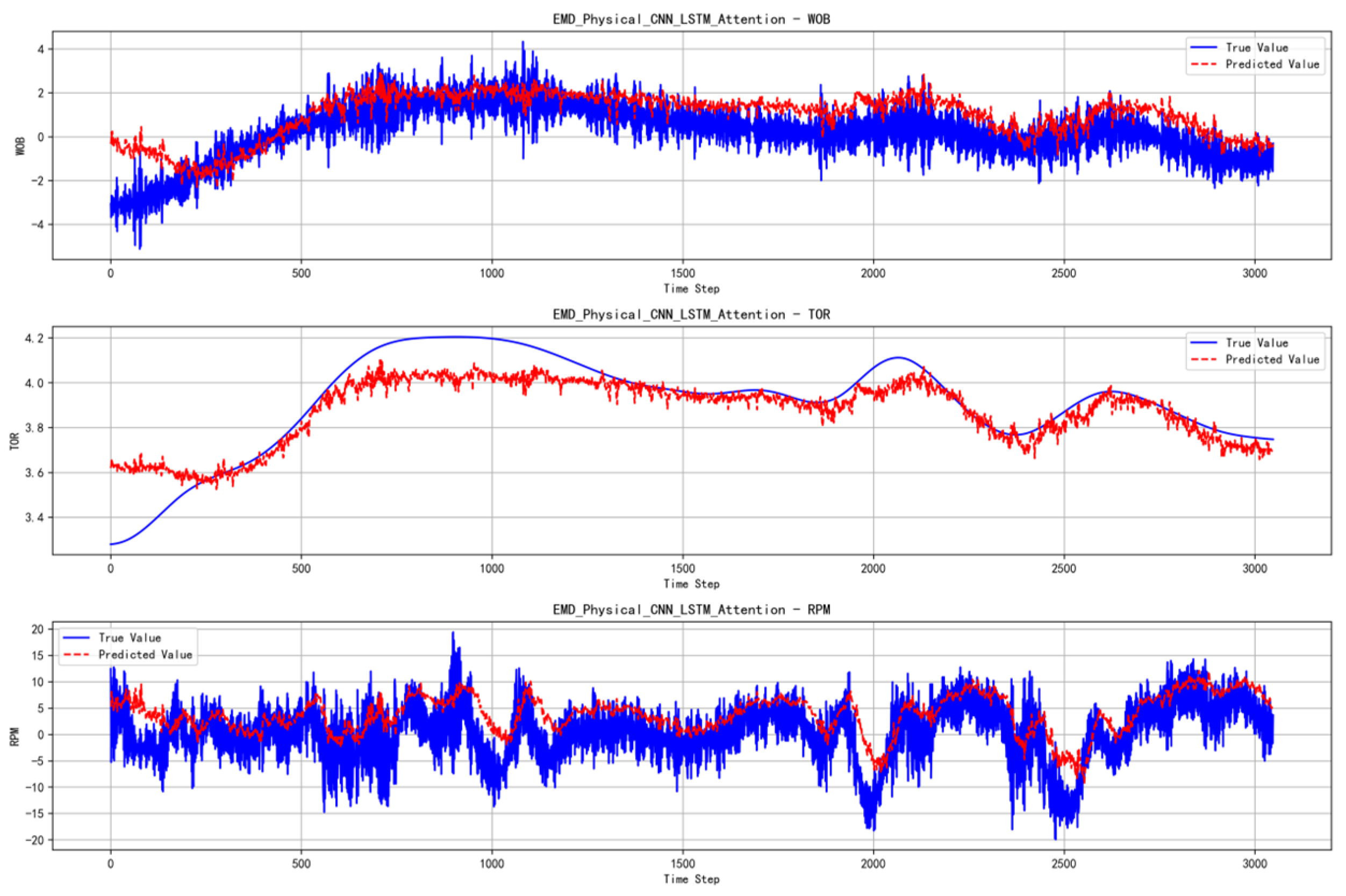
As shown in Figure 18 and Figure 19, before the introduction of physical constraints, the EMD + CNN-LSTM-Attention model’s predicted data deviated significantly from the true data. After incorporating physical constraints, the difference between the predicted and true data improved somewhat, but the prediction performance did not enhance significantly. Especially during torque testing, when the prediction results were already relatively good, the difference in prediction performance before and after the introduction of physical constraints was minimal.

Figure 18.
Prediction performance of the EMD—CNN-LSTM-Attention model.

Figure 19.
Prediction performance of the EMD—Physical—CNN-LSTM-Attention model.
This experiment, starting from data-driven deep learning models and incorporating the method of physical constraints, has successfully achieved high-precision modeling of a multivariable complex dynamic system. The experimental results show that the introduction of physical constraints not only effectively reduces prediction errors but also significantly enhances the model’s generalization ability and stability, providing new ideas and methods for the dynamic modeling of complex systems. Future research can further expand to more scenarios involving multivariable coupling, exploring the generalization ability and application potential of physical constraints.
4.3.2. The Impact of EMD and VMD on the Model
In this study, we investigated the effects of Empirical Mode Decomposition (EMD) and Variational Mode Decomposition (VMD) on drilling parameter prediction models, particularly their application performance in predicting WOB, TOR, and RPM. By comparing models using different data decomposition methods (EMD + CNN-LSTM-Attention and VMD + CNN-LSTM-Attention) and their versions enhanced with physical mechanisms, we analyzed the differences in the performance of the two modal decomposition methods within deep learning models and their impact on prediction accuracy.
Firstly, EMD has certain limitations when dealing with non-stationary signals, especially in more complex signal decomposition tasks. EMD decomposes signals empirically into Intrinsic Mode Functions (IMFs) and is sometimes susceptible to mode mixing issues, which can prevent the accurate separation of more complex or high-frequency signal components. This is particularly evident in the prediction of drilling pressure and rotational speed. As shown in Table 6, in WOB prediction, the R2 value of the EMD model is relatively low at 0.4131, indicating weaker data interpretability and larger prediction errors. In contrast, VMD, as a more advanced modal decomposition method, can better handle the non-stationarity and complexity of signals. VMD decomposes signals through an optimization problem, effectively avoiding mode mixing and maintaining the independence of signal components, thereby providing more accurate feature extraction. This is especially true in the prediction tasks of WOB and RPM, where VMD significantly improves model performance. For example, in WOB prediction, the R2 value of the VMD combined with CNN-LSTM model increases to 0.5715, an improvement of about 0.16 compared to EMD. In RPM prediction, the R2 value of the VMD model reaches as high as 0.8581, demonstrating its advantage in complex signal modeling.
Table 6.
Model comparison.
As shown in Table 7, under the same physical constraint conditions, in WOB prediction, the R2 value of VMD combined with physical mechanisms reaches 0.8636, significantly higher than the 0.5183 of the EMD model. This shows that the introduction of physical mechanisms substantially enhances the prediction capability of the VMD model. In TOR prediction, both EMD and VMD models exhibit relatively good predictive performance, and the introduction of physical mechanisms further improves prediction accuracy. However, the advantages of the VMD model remain more pronounced, especially after incorporating physical mechanisms. The MSE and MAE indicators are improved, and the R2 value increases to 0.9128, indicating that VMD can provide more precise results in torque prediction tasks.
Table 7.
Model comparison.
Overall, VMD demonstrates a clear advantage over EMD in the prediction of WOB, especially in handling complex signals. VMD is able to provide more accurate signal decomposition and reduce prediction errors. Additionally, the incorporation of physical mechanisms significantly enhances the model’s predictive capabilities, particularly in the prediction of WOB and RPM, further strengthening the model’s understanding and fitting ability of the physical processes. Therefore, the combination of VMD and physical mechanisms offers a more reliable and precise solution for the prediction of drilling parameters and is worthy of further promotion and application in practical scenarios.
4.3.3. Comprehensive Comparison
- Performance of the VMD + CNN-LSTM-Attention + Physical Model
VMD is a nonlinear method based on signal decomposition, capable of breaking down complex signals into multiple Intrinsic Mode Functions. This allows VMD to capture multi-level information within the signal, giving it an advantage in handling nonlinear and non-stationary signals. This is especially true for drilling data, which has complex time-varying characteristics. VMD can effectively decompose and extract useful features from such signals [32].
The combination of VMD + CNN-LSTM-Attention model leverages the strengths of VMD in signal decomposition, the feature extraction capabilities of Convolutional Neural Networks, the time-series modeling abilities of LSTM networks, and the weight adjustment capabilities of the Attention mechanism. This forms a powerful multi-level, multi-model collaborative prediction system. As a result, the VMD model achieves the best performance in terms of MSE, MAE, and R2, especially for parameters like WOB and TOR.
This model incorporates physical mechanism constraints based on VMD. Integrating physical knowledge typically enhances the model’s prediction accuracy because it enables the model to better capture the physical laws involved in the drilling process. This improves the fit of drilling parameters, especially for complex variables like RPM and TOR. After incorporating physical mechanisms, the model can better constrain its output, resulting in smaller prediction errors, higher R2 values, and reduced MSE and MAE.
- 2.
- Performance of the Transform Model
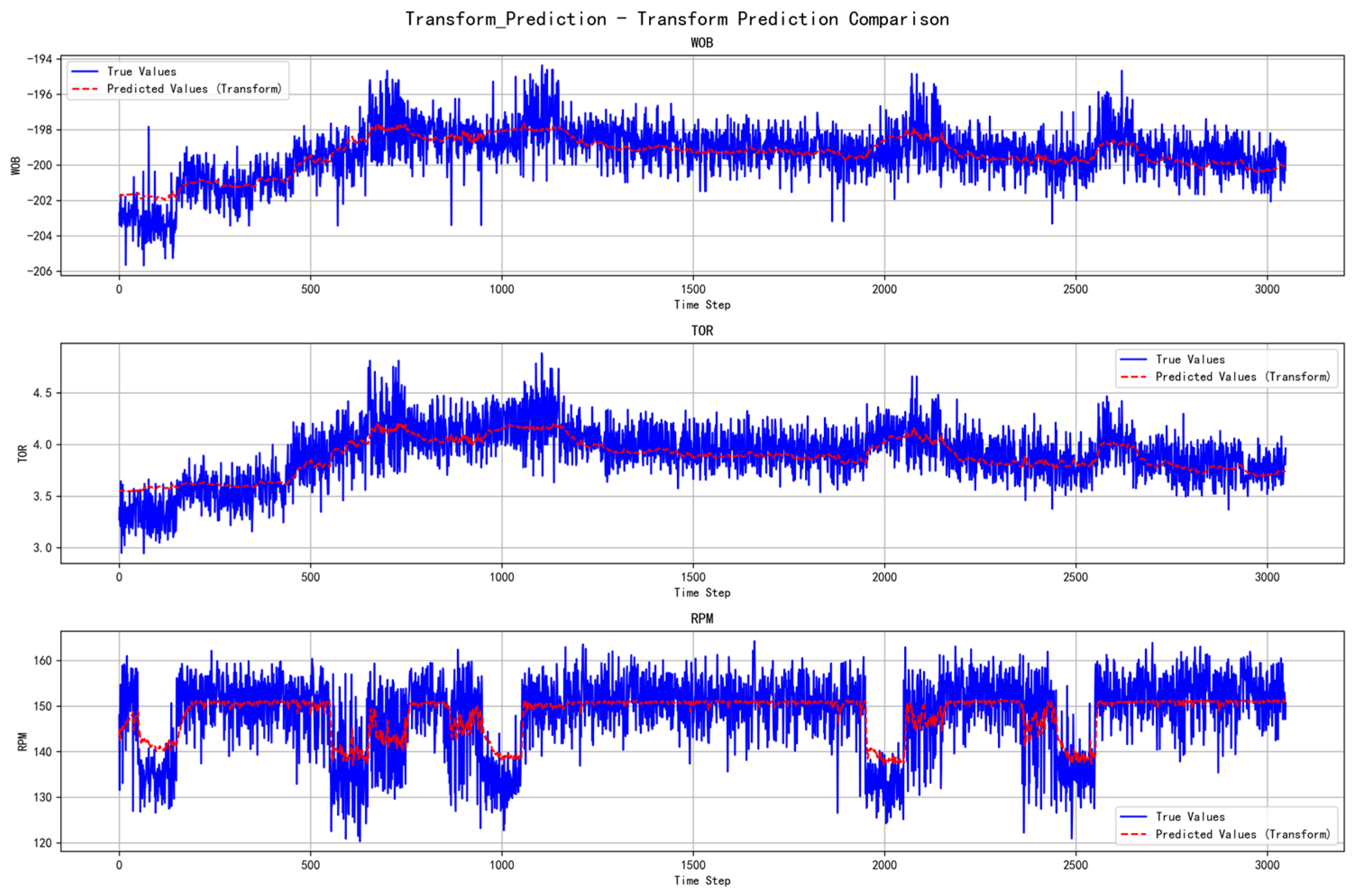
The Transform model, as a technique based on transformation, can effectively perform feature transformation and modeling to some extent. As shown in Figure 20, compared to complex deep learning models like VMD + CNN-LSTM-Attention, it lacks the ability to capture fine-grained features of complex signals. Therefore, while the Transform model performs well in some scenarios, its prediction accuracy is inferior to the VMD model when dealing with complex drilling data. Additionally, the Transform model lacks in-depth exploration of temporal characteristics. Unlike LSTM, it cannot remember long-term historical information, nor does it have an Attention mechanism to dynamically adjust importance weights. This affects its prediction accuracy for complex variables such as RPM and TOR.
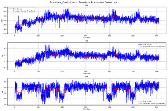
Figure 20.
Prediction performance of the Transform model.
- 3.
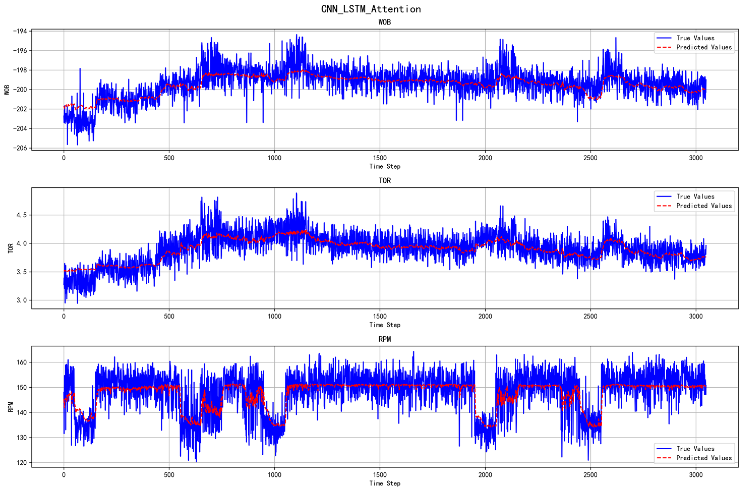
- Performance of the CNN-LSTM-Attention Model
CNN is used to automatically extract local features, while LSTM captures long-term dependencies [33,34]. In theory, such models can handle complex time-series data. As shown in Figure 21, without physical mechanism constraints, the model’s performance may not be optimal, as it cannot fully understand the physical laws of the drilling process and relies solely on the patterns within the data for training. The Attention mechanism can help the model focus on the most important moments and features, which is crucial for complex time-varying signals in the drilling process. Nevertheless, even though Attention can significantly enhance model performance, it still falls short compared to the VMD model with physical mechanisms.
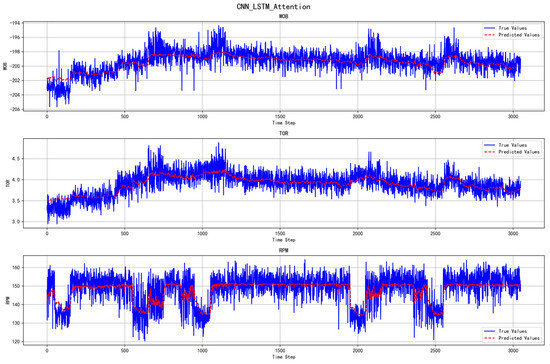
Figure 21.
Prediction performance of the CNN-LSTM-Attention model.
- 4.
- Disadvantages of the EMD Model
EMD is also an effective signal decomposition method. However, when dealing with complex nonlinear signals, it may not decompose the intrinsic modes of the signal as precisely as VMD. EMD has weaker local feature extraction capabilities, especially when processing highly non-stationary drilling data. Its decomposition results may be affected by noise, leading to poor prediction performance.
Although EMD + CNN-LSTM-Attention + Physical model incorporates physical mechanisms based on EMD, the inherent limitations of EMD still result in inferior performance compared to the VMD model. The limited capability of EMD to effectively extract complex features from the data compromises the model’s fitting performance, resulting in relatively high MSE and MAE values and a lower R2.
- 5.
- The superiority of deep learning over traditional filtering methods in data preprocessing
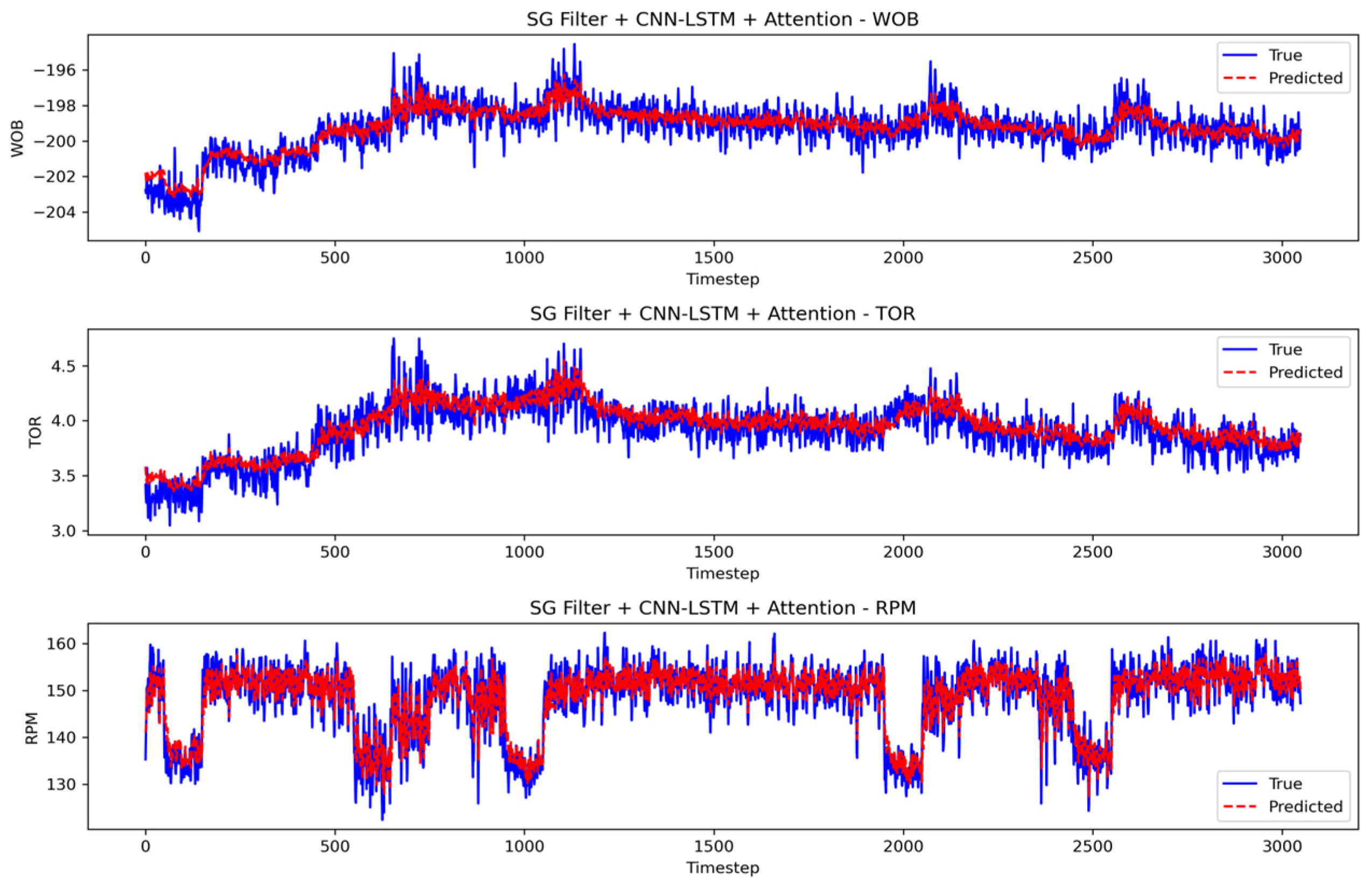
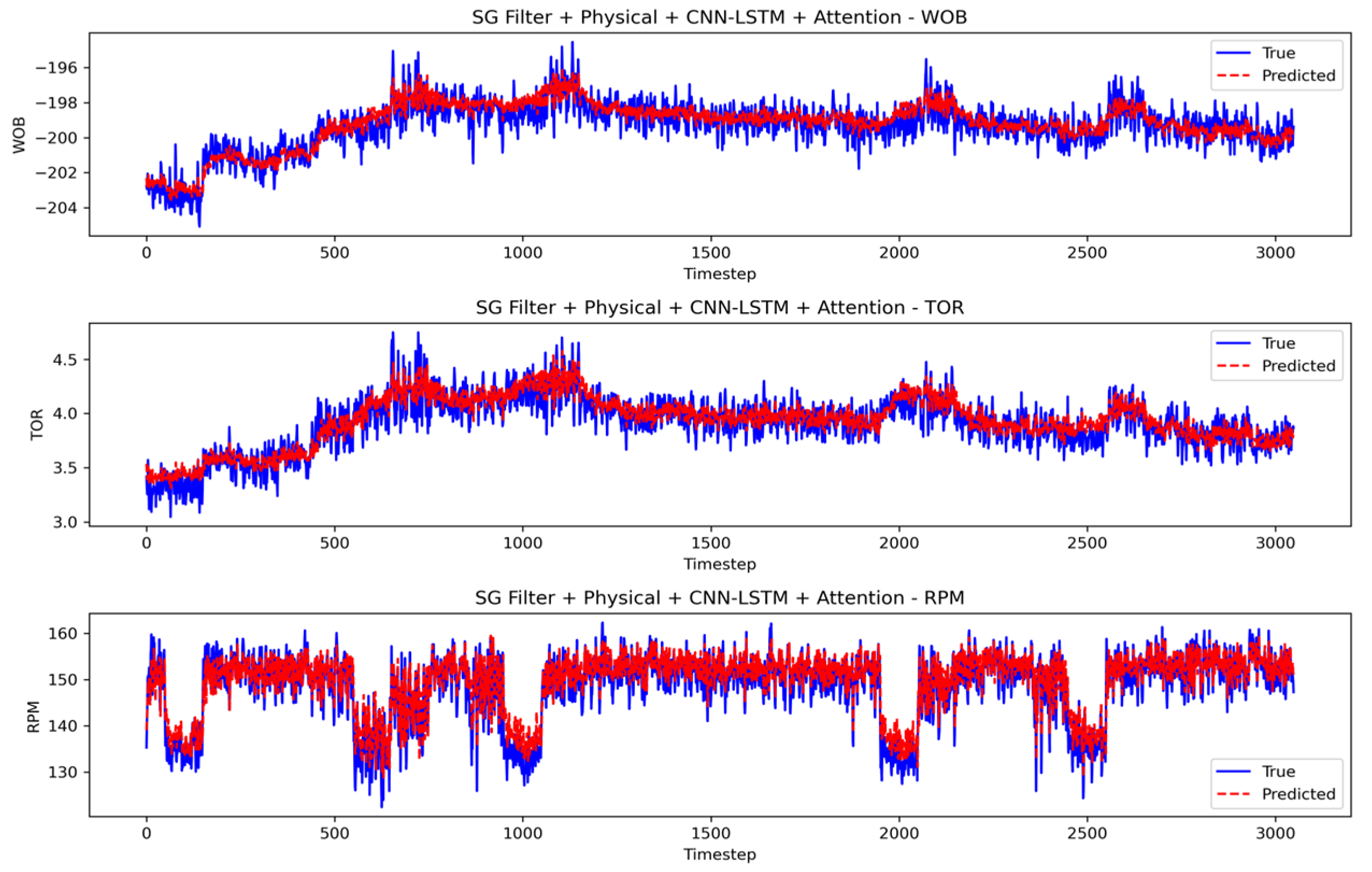
As shown in the comparison between Table 4 and Table 8. Compared to traditional filtering methods such as Savitzky–Golay (SG) and Variational Mode Decomposition (VMD), deep learning-based preprocessing exhibits clear advantages in capturing complex, nonlinear patterns and enhancing model performance. As shown in the experimental results, the SG + CNN-LSTM-Attention method yields relatively high errors, particularly in RPM prediction (MSE = 11.4169, R2 = 0.7128), indicating limited capacity in noise suppression and feature retention. In contrast, when physical constraints are incorporated, the SG-based model shows moderate improvement (R2 = 0.7968 for RPM) but still lags behind VMD-based approaches.
Table 8.
Model comparison.
As shown in Figure 22 and Figure 23, the VMD + Physical + CNN-LSTM-Attention model achieves the best overall performance across all parameters (e.g., R2 = 0.9801 for RPM and 0.9128 for TOR), demonstrating the deep model’s ability to integrate domain knowledge and extract meaningful components from decomposed signals. This result highlights that while traditional filtering can provide a basic level of signal smoothing, deep learning models not only enhance denoising but also adaptively learn task-relevant representations, thereby offering superior data preprocessing capabilities.
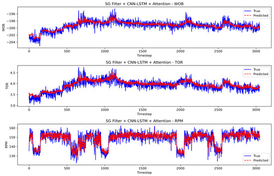
Figure 22.
Prediction performance of the SG + CNN-LSTM-Attention model.
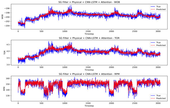
Figure 23.
Prediction performance of the SG + Physical + CNN-LSTM-Attention model.
- 6.
- Multi-step Prediction and Practical Significance
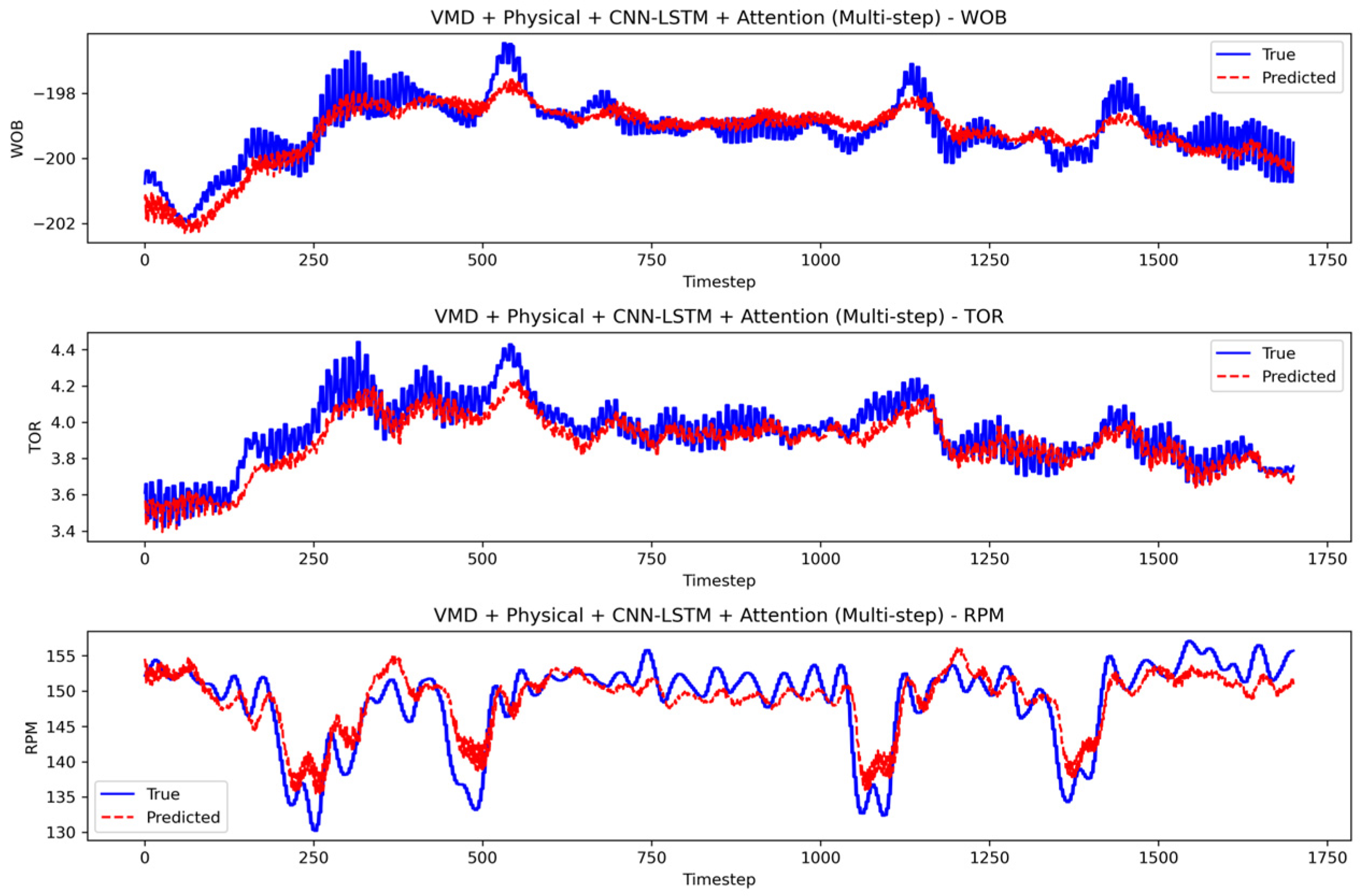
To address the potential limitations of single-step prediction (typically 1–5 s ahead), this study further introduces a multi-step forecasting experiment, extending the prediction horizon to three steps (approximately 15 s). This adjustment aims to better align the model with real-world requirements for advance warning, especially in high-risk formations, deep well drilling, or complex load conditions where the early detection of abnormal trends can enable timely operational interventions and reduce the risk of stuck pipe incidents.
Built upon the “VMD + Physical + CNN-LSTM + Attention” framework, the multi-step prediction experiment demonstrates that the model maintains robust performance even over an extended time window.
As show in Table 9 and Figure 24, these results suggest that the proposed model is capable not only of short-term trend learning, but also of effectively predicting the dynamic behavior of drilling parameters several seconds in advance. This enhances its value as a practical early warning and decision-support tool in intelligent drilling operations.
Table 9.
Model comparison.
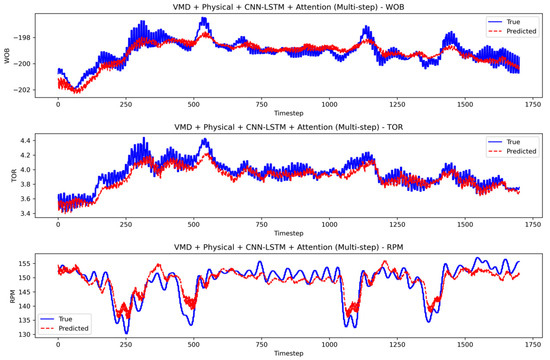
Figure 24.
Prediction performance of the VMD + Physical + CNN-LSTM + Attention (multi-step) model.
5. Conclusions
- (1)
- Through time domain, frequency domain, time-frequency domain, and vibration analysis of near-bit downhole data, no significant characteristics were found before and after a stuck pipe event. Modal decomposition methods were employed to extract features, which were then used as inputs for the model.
- (2)
- In response to the limitations of the three common approaches in previous stuck pipe prediction studies—simple rule-based, physics-based, and data-driven methods—a more efficient model based on modal decomposition of near-bit data with physical constraints was proposed.
- (3)
- By comparing the six models and evaluating their performance metrics, it was found that the VMD + CNN-LSTM-Attention + Physical model achieved the best prediction results, with an R2 value reaching approximately 0.9, significantly outperforming other algorithms.
- (4)
- When applied to actual drilling operations, the model can effectively detect early signals of stuck pipe events and prevent stuck pipe accidents. It facilitates the implementation of timely and effective corrective measures, thereby reducing the occurrence of downhole incidents.
Author Contributions
Conceptualization, T.Z. and Y.X.; methodology, Y.X.; software, Z.M.; validation, T.Z., Y.X. and W.Z.; formal analysis, W.Z.; investigation, M.S.; resources, T.Z.; data curation, T.Z.; writing—original draft preparation, Y.X.; writing—review and editing, Z.M.; visualization, Y.X.; supervision, J.L.; project administration, T.Z. and J.L. All authors have read and agreed to the published version of the manuscript.
Funding
This research was funded by the National Natural Science Foundation of China-Maior Scientific Research Instrument Project, grant number 52227804, General Program of National Natural Science Foundation of China, grant number 52274003.
Data Availability Statement
The data that support the findings of this study are available from the author Tao-Zhang (zt@bistu.edu.cn) upon reasonable request.
Conflicts of Interest
The authors declare no conflicts of interest.
References
- Li, Q.; Li, Q.; Han, Y. A numerical investigation on kick control with the displacement kill method during a well test in a deep-water gas reservoir: A case study. Processes 2024, 12, 2090. [Google Scholar] [CrossRef]
- Li, Q.; Li, Q.; Wu, J.; Li, X.; Li, H.; Cheng, Y. Wellhead stability during development process of hydrate reservoir in the Northern South China Sea: Evolution and mechanism. Processes 2024, 13, 40. [Google Scholar] [CrossRef]
- Kaneko, T.; Inoue, T.; Nakagawa, Y.; Wada, R.; Abe, S.; Yasutake, G.; Fujita, K. Hybrid Approach Using Physical Insights and Data Science for Stuck-Pipe Prediction. SPE J. 2024, 29, 641–650. [Google Scholar] [CrossRef]
- Fernandez, B.M. Estimation of the Free Rotating Hook Load for WOB Estimation. Master’s Thesis, UIS, Springfield, IL, USA, 2022. Available online: https://hdl.handle.net/11250/3018193 (accessed on 20 November 2024).
- Esmael, B.; Arnaout, A.; Fruhwirth, R.; Thonhauser, G. A statistical feature-based approach for operations recognition in drilling time series. Int. J. Comput. Inf. Syst. Ind. Manag. Appl. 2012, 4, 100–108. [Google Scholar]
- Agrawal, R.; Malik, A.; Samuel, R.; Saxena, A. Real-time prediction of Litho-facies from drilling data using an Artificial Neural Network: A comparative field data study with optimizing algorithms. J. Energy Resour. Technol. 2022, 144, 043003. [Google Scholar] [CrossRef]
- Montes, A.C.; Pradeepkumar, A.; Eric, V.O. Review of Stuck Pipe Prediction Methods and Future Directions. In Proceedings of the SPE Annual Technical Conference and Exhibition, Dallas, TX, USA, 6–8 October 2024. [Google Scholar] [CrossRef]
- Zhu, S.; Song, X.; Zhu, Z.; Yao, X.; Liu, M. Intelligent prediction of stuck pipe using combined data-driven and knowledge-driven model. Appl. Sci. 2022, 12, 5282. [Google Scholar] [CrossRef]
- Oyedere, M.O. Improved Torque and Drag Modeling Using Traditional and Machine Learning Methods. Diss. 2020. Available online: https://hdl.handle.net/2152/115839 (accessed on 20 November 2024).
- Zhou, Y. Data-Driven Drilling Optimization and Field Development in Unconventionals. Diss. 2019. Available online: https://hdl.handle.net/2152/88680 (accessed on 20 November 2024).
- Zhang, F.; Islam, A.; Zeng, H.; Chen, Z.; Zeng, Y.; Wang, X.; Li, S. Real time stuck pipe prediction by using a combination of physics-based model and data analytics approach. In Proceedings of the Abu Dhabi International Petroleum Exhibition and Conference, Abu Dhabi, United Arab Emirates, 11–14 November 2019. [Google Scholar] [CrossRef]
- Agwu, O.E.; Akpabio, J.U.; Alabi, S.B.; Dosunmu, A. Artificial intelligence techniques and their applications in drilling fluid engineering: A review. J. Pet. Sci. Eng. 2018, 167, 300–315. [Google Scholar] [CrossRef]
- Hussain, B.; Du, Q.; Ren, P. Semi-supervised learning based big data-driven anomaly detection in mobile wireless networks. J. China Commun. 2018, 15, 41–57. [Google Scholar] [CrossRef]
- Wang, T.; Qiao, M.; Zhang, M.; Yang, Y.; Snoussi, H. Data-driven prognostic method based on self-supervised learning approaches for fault detection. J. Intell. Manuf. 2020, 31, 1611–1619. [Google Scholar] [CrossRef]
- Xu, H.; Sun, Z.; Cao, Y.; Bilal, H. A data-driven approach for intrusion and anomaly detection using automated machine learning for the Internet of Things. J. Soft Comput. 2023, 27, 14469–14481. [Google Scholar] [CrossRef]
- Taqvi, S.A.A.; Zabiri, H.; Tufa, L.D.; Uddin, F.; Fatima, S.A.; Maulud, A.S. A review on data-driven learning approaches for fault detection and diagnosis in chemical processes. ChemBioEng Rev. 2021, 8, 239–259. [Google Scholar] [CrossRef]
- Woldaregay, A.Z.; Årsand, E.; Botsis, T.; Albers, D.; Mamykina, L.; Hartvigsen, G. Data-driven blood glucose pattern classification and anomalies detection: Machine-learning applications in type 1 diabetes. J. Med. Internet Res. 2019, 21, e11030. Available online: https://preprints.jmir.org/preprint/11030 (accessed on 25 November 2024). [CrossRef] [PubMed]
- Daubechies, I.; Lu, J.; Wu, H.T. Synchrosqueezed wavelet transforms: An empirical mode decomposition-like tool. Appl. Comput. Harmon. Anal. 2011, 30, 243–261. [Google Scholar] [CrossRef]
- Gilles, J. Empirical wavelet Transform. IEEE Trans. Signal Process. 2013, 61, 3999–4010. [Google Scholar] [CrossRef]
- Huang, N.E.; Shen, Z.; Long, S.R.; Wu, M.C.; Shih, H.H.; Zheng, Q.; Yen, N.-C.; Tung, C.C.; Liu, H.H. The empirical mode decomposition and the Hilbert spectrum for nonlinear and non-stationary time series analysis. Proc. R. Soc. London Ser. A Math. Phys. Eng. Sci. 1998, 454, 903–995. [Google Scholar] [CrossRef]
- Sharpley, R.C. Analysis of the intrinsic mode functions. Constr. Approx. 2006, 24, 17–47. [Google Scholar] [CrossRef]
- Wang, Y.-Q.; Gao, Y.-S.; Liu, J.-M.; Liu, C. Explicit formula for the Liutex vector and physical meaning of vorticity based on the Liutex-Shear decomposition. J. Hydrodyn. 2019, 31, 464–474. [Google Scholar] [CrossRef]
- Ben Ali, J.; Fnaiech, N.; Saidi, L.; Chebel-Morello, B.; Fnaiech, F. Application of empirical mode decomposition and artificial neural network for automatic bearing fault diagnosis based on vibration signals. Appl. Acoust. 2015, 89, 16–27. [Google Scholar] [CrossRef]
- Andrade, A.O.; Kyberd, P.; Nasuto, S.J. The application of the Hilbert spectrum to the analysis of electromyographic signals. Inf. Sci. 2008, 178, 2176–2193. [Google Scholar] [CrossRef]
- Chen, H.; Wu, H.; Kan, T.; Zhang, J.; Li, H. Low-carbon economic dispatch of integrated energy system containing electric hydrogen production based on VMD-GRU short-term wind power prediction. Int. J. Electr. Power Energy Syst. 2023, 154, 109420. [Google Scholar] [CrossRef]
- Bai, S.; Kolter, J.Z.; Koltun, V. An empirical evaluation of generic convolutional and recurrent networks for sequence modeling. arXiv 2018, arXiv:1803.01271. [Google Scholar] [CrossRef]
- Ma, J.; Huo, M.; Han, J.; Liu, Y.; Lu, S.; Yu, X. Integrated CNN-LSTM for Photovoltaic Power Prediction based on Spatio-Temporal Feature Fusion. Eng. Rep. 2025, 7, e13088. [Google Scholar] [CrossRef]
- Hochreiter, S.; Schmidhuber, J. Long short-term memory. J. Neural Comput. 1997, 9, 1735–1780. [Google Scholar] [CrossRef] [PubMed]
- de Moura, J.; Xiao, Y.; Yang, J.; Butt, S.D. An empirical model for the drilling performance prediction for roller-cone drill bits. J. Pet. Sci. Eng. 2021, 204, 108791. [Google Scholar] [CrossRef]
- Gomes, D.; Jaritz, T.; Robinson, T.S.; and Revheim, O.E. Enhancing Stuck Pipe Risk Detection in Exploration Wells Using Machine Learning Based Tools: A Gulf of Mexico Case Study. In Proceedings of the IADC/SPE International Drilling Conference and Exhibition, Galveston, TX, USA, 5–7 March 2024. [Google Scholar] [CrossRef]
- Zhu, X.; Cheng, D.; Zhang, Z.; Lin, S.; Dai, J. An empirical study of spatial attention mechanisms in deep networks. In Proceedings of the IEEE/CVF International Conference on Computer Vision, Seoul, Republic of Korea, 27 October–2 November 2019. [Google Scholar]
- Lian, J.; Liu, Z.; Wang, H.; Dong, X. Adaptive variational mode decomposition method for signal processing based on mode characteristic. J. Mech. Syst. Signal Process. 2018, 107, 53–77. [Google Scholar] [CrossRef]
- Ullah, W.; Ullah, A.; Haq, I.U.; Muhammad, K.; Sajjad, M.; Baik, S.W. CNN features with bi-directional LSTM for real-time anomaly detection in surveillance networks. Multimed. Tools Appl. 2021, 80, 16979–16995. [Google Scholar] [CrossRef]
- Lai, G.; Chang, W.C.; Yang, Y.; Liu, H. Modeling long-and short-term temporal patterns with deep neural networks. In Proceedings of the 41st International ACM SIGIR Conference on Research & Development in Information Retrieval, Ann Arbor, MI, USA, 8–12 July 2018; pp. 95–104. [Google Scholar] [CrossRef]


Disclaimer/Publisher’s Note: The statements, opinions and data contained in all publications are solely those of the individual author(s) and contributor(s) and not of MDPI and/or the editor(s). MDPI and/or the editor(s) disclaim responsibility for any injury to people or property resulting from any ideas, methods, instructions or products referred to in the content. |
© 2025 by the authors. Licensee MDPI, Basel, Switzerland. This article is an open access article distributed under the terms and conditions of the Creative Commons Attribution (CC BY) license (https://creativecommons.org/licenses/by/4.0/).