Real-Time Prediction of Wear Morphology and Coefficient of Friction Using Acoustic Signals and Deep Neural Networks in a Tribological System

Abstract

Predicting real-time wear depth distribution and the coefficient of friction (COF) in tribological systems is challenging due to the dynamic and complex nature of surface interactions, particularly influenced by surface roughness. Traditional methods, relying on post-test measurements or oversimplified assumptions, fail to capture this dynamic behavior, limiting their utility for real-time monitoring. To address this, we developed a deep neural network (DNN) model by integrating experimental tribological testing and finite element method (FEM) simulations, using acoustic signals for non-invasive, real-time analysis. Experiments with brass pins (UNS C38500) of varying surface roughness (240, 800, and 1200 grit) sliding against a 304 stainless steel disc provided data to validate the FEM model and train the DNN. The DNN model predicted wear morphology with accuracy comparable to FEM simulations but at a lower computational cost, and the COF with relative errors below 10% compared to experimental measurements. This approach enables real-time monitoring of wear and friction, offering significant benefits for predictive maintenance and operational efficiency in industrial applications.

1. Introduction

Tribology, the science of friction, wear, and lubrication, is fundamental to the performance and durability of mechanical systems across diverse industries, including automotive, aerospace, and manufacturing [1,2,3,4,5,6,7,8,9,10,11]. The interaction between sliding surfaces, particularly the influence of surface roughness, governs critical phenomena such as wear rates, frictional forces, and acoustic emissions [12,13,14,15,16,17,18,19]. Understanding these interactions is essential for optimizing system efficiency, reducing energy losses, and extending component lifespan. Recent advancements in computational modeling and machine learning have introduced new possibilities for analyzing and predicting tribological behavior, offering non-invasive and efficient alternatives to traditional experimental methods [20,21,22,23,24,25,26,27,28,29].

Prior studies have extensively investigated the relationship between surface roughness and tribological performance. Abdelounis et al. [30] employed the finite element software ABAQUS to simulate friction noise between two rough, dry surfaces. Their findings indicate that the vibratory level, Lv (dB), increases linearly with the logarithm of both surface roughness and sliding speed, consistent with our experimental results. Lontin et al. [31] modeled surface asperities as beams, positing that their vibration generates noise following impact. However, their approach considers only tangential forces to determine wear and vibration, omitting normal forces, which conflicts with the widely accepted Archard model. Basit et al. [32,33] developed an analytical ball-on-disc model to explore the link between friction noise and wear evolution. Yet, their model oversimplifies the system by attributing friction noise solely to the ball’s vibration, neglecting contributions from the disc. Similarly, Tian et al. [34] derived a quantitative equation relating wear volume, the COF, and noise signals using symbolic regression. This method, however, requires dynamic COF and acoustic signals as inputs to predict wear volume, limiting its practical utility. Moreover, these approaches provide only wear volume estimates, failing to capture real-time wear depth distribution or COF.

Recent research has also leveraged deep learning for tool wear prediction. Huang et al. [35] utilized a Deep Convolutional Neural Network (DCNN) to fuse multi-domain features from multisensory signals, enabling real-time tool wear prediction. Cai et al. [36] employed a Long Short-Term Memory (LSTM) network to extract features from multisensor time-series data, integrating them with process information for wear prediction across various conditions. Sun et al. [37] combined an LSTM network with a residual convolutional neural network (ResNet) to forecast tool wear conditions during machining. Xu et al. [38] enhanced prediction accuracy by incorporating multi-scale feature fusion and a channel attention mechanism into their deep neural network (DNN). He et al. [39] predicted tool wear using temperature signals processed through DNN. However, these studies focus primarily on predicting wear conditions or values rather than the detailed morphology of wear. To the best of the authors’ knowledge, no prior research has employed DNN modeling to continue to predict wear depth distribution and COF based on acoustic signals.

This study addresses these gaps by developing an integrated framework that combines experimental tribological testing and finite element method (FEM) simulations to train a DNN model. This model predicts wear morphology and COF during frictional sliding. We investigate the role of initial surface roughness using brass pins (UNS C38500) polished with varying grit sizes (240, 800, and 1200) slid against a 304 stainless steel disc. A key innovation of our approach is the use of acoustic signals as the primary input for predictive modeling, enabling real-time monitoring of wear and COF.

This study not only enhances the understanding of roughness-dependent tribological interactions but also represents the first implementation of DNN methodology to predict COF and wear depth through acoustic signals. Specifically, this research examines the effect of surface roughness on wear development, COF, and frictional noise, emphasizing the use of acoustic signals to predict tribological behavior. Tribological tests were conducted under controlled conditions, capturing acoustic emissions alongside wear and friction data. These experimental results validated an FEM model simulating wear evolution, which provided inputs for the DNN. The DNN was trained to predict worn surface morphology and COF using acoustic noise, wear coefficients, and temporal data, achieving high accuracy compared to experimental and FEM results.

This paper is structured as follows: Section 2 outlines the methodology, including sample preparation, tribological testing, FEM modeling, and DNN development. Section 3 presents the results and discussion, covering surface roughness measurements, COF trends, acoustic signal analysis, wear profiles, and DNN predictions. Section 4 concludes this study with key findings and implications for future research, underscoring the methodology’s potential for real-time wear monitoring in industrial systems.

2. Materials and Methods

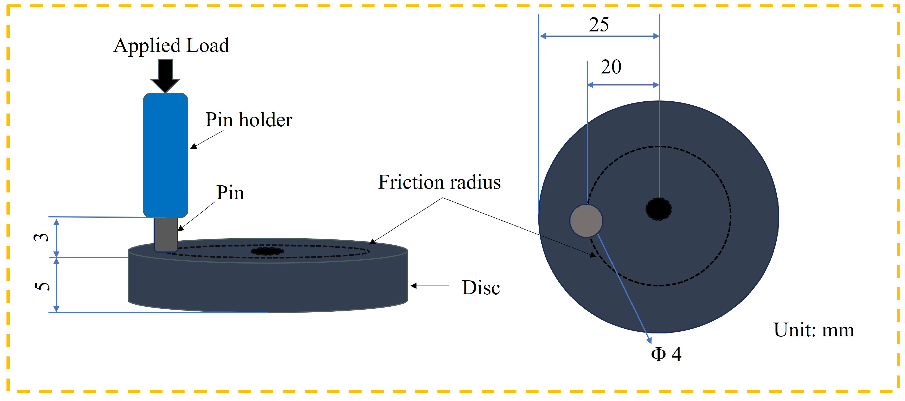
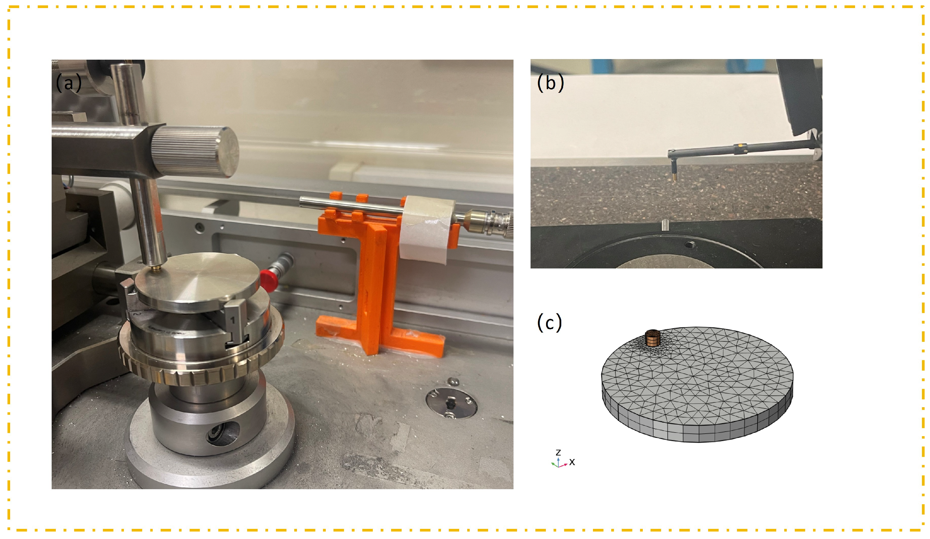
2.1. Sample Preparation and Tribological Testing

Cylindrical pins were fabricated from UNS C38500 brass and polished sequentially using sandpaper with grit sizes of 240, 800, and 1200 to achieve a smooth surface finish. The pins, cylindrical in shape, have a length of 3 mm and a diameter of 4 mm, as shown in Figure 1. Tribological tests involved sliding the pins against a 304 stainless steel disc (diameter: 25 mm) under a 20 N load at a speed of 0.84 m/s for 1 min. The sliding track was 20 mm from the disc’s center. Each test condition was repeated five times for the same roughness level to ensure repeatability. A GRAS free-field pressure microphone with a maximum operating frequency of 20 kHz was used to record sound emissions from the tribometer resulting from the friction process, as shown in Figure 2a. The microphone was calibrated using a GRAS pistonphone type 42AA at 23 °C, 36% relative humidity, and 986 hPa barometric pressure, achieving a sensitivity of 47.46 mV/Pa with an accuracy of ±0.1 mV/Pa. The microphone, positioned 10 cm from the pin–disc interface, was directly connected to an NI 9350 data acquisition (DAQ) card without a preamplifier, since the input impedance of the DAQ card matched the output impedance of the microphone. The DAQ card operated at a sampling rate of 25.6 kHz. A built-in low-pass filter with a cut-off frequency of 20 kHz was applied to target human-audible noise in this study. Measurements were conducted in a temperature-controlled laboratory (23 °C ± 1 °C) free from other noise sources. The sound pressure measurement accuracy was ±0.003 Pa, enabling reliable analysis of friction and wear behavior.

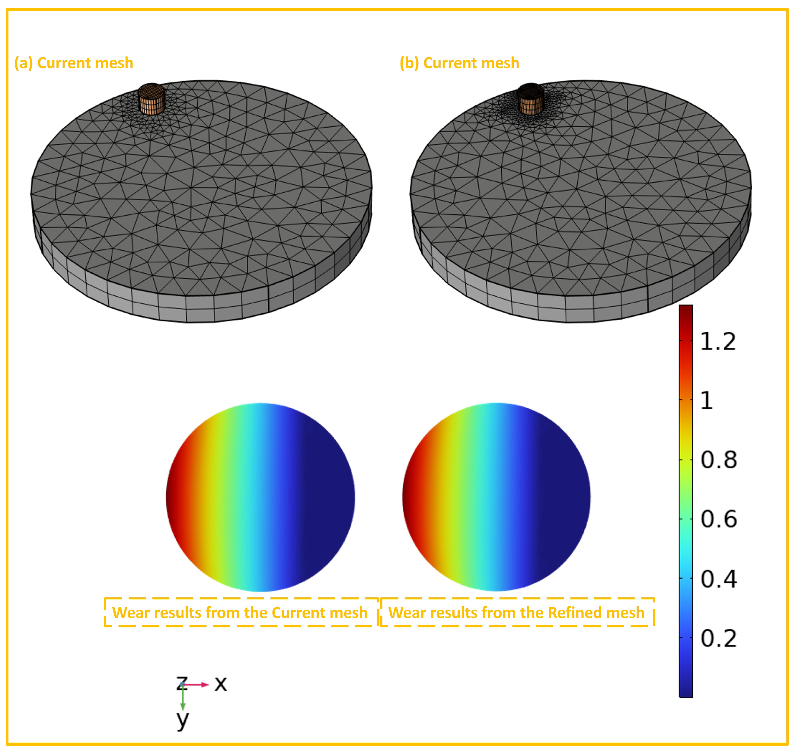
2.2. Wear Measurement and Finite Element Modeling

Due to the short duration of the wear tests, direct measurement of wear loss via mass difference before and after testing was deemed impractical. Instead, wear morphology was analyzed using a profilometer, as illustrated in Figure 2b. The wear loss and wear coefficient (WOF) were subsequently calculated using the Archard wear model. To simulate wear development, a finite element method (FEM) model was implemented in COMSOL Multiphysics 6.3 , with the setup depicted in Figure 2c. The disc was meshed using a free triangular mesh with 1134 elements to facilitate refinement at the contact region with the pin. The pin was meshed using a free quadrilateral mesh with 384 elements to enhance computational efficiency. The material properties are presented in

Table 1. Material properties of steel and brass.

Material	Density (kg/m3)	Young’s Modulus (Pa)	Poisson’s Ratio
Steel	7860	1.9984 × 1011	0.24
Brass	8469.3	9.8 × 1010	0.32

. The FEM model was validated by comparing the simulated wear surface morphology with experimentally measured surface morphology, ensuring its accuracy was sufficient to train the DNN model.

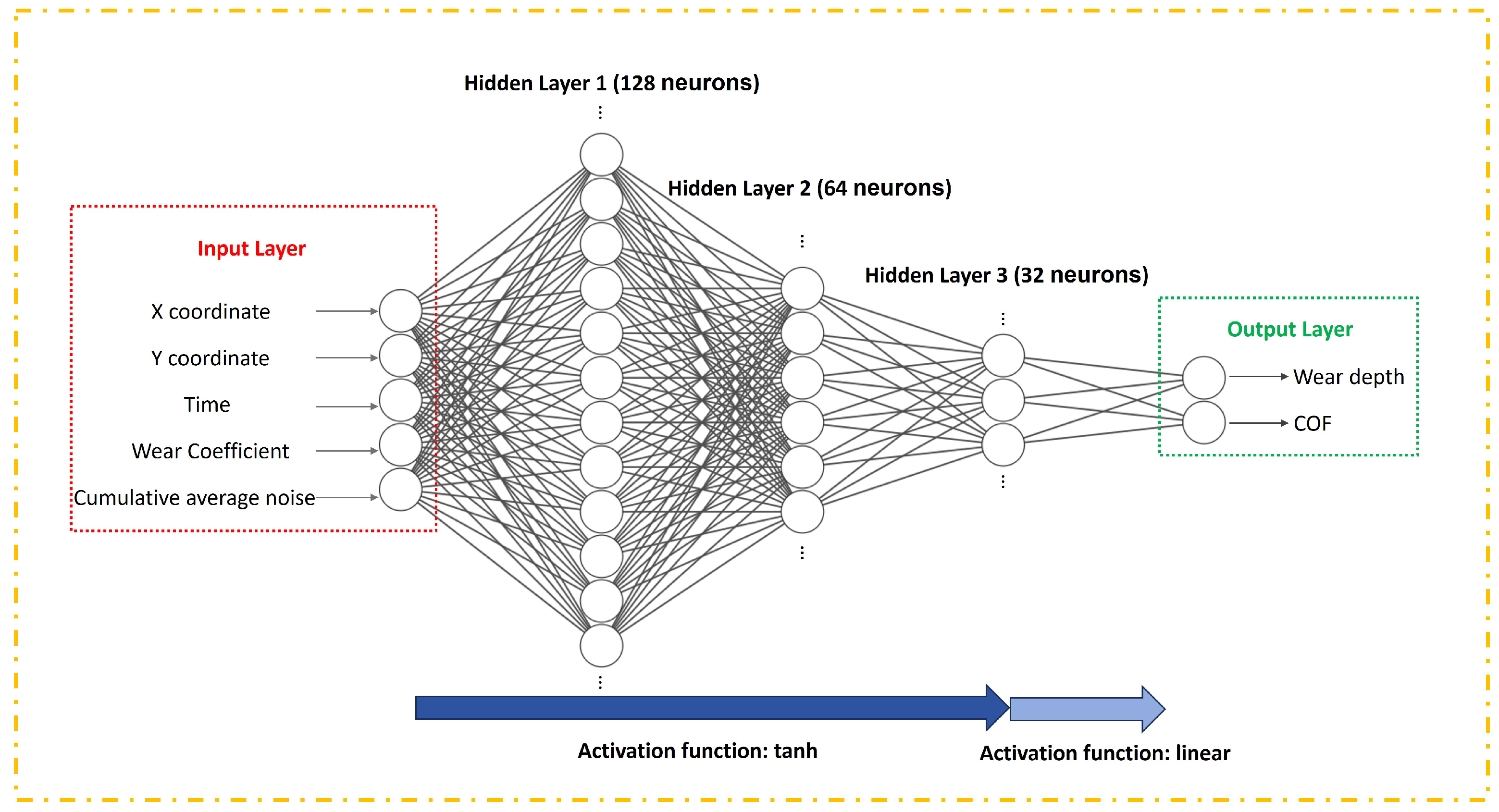
2.3. Deep Neural Network Model Development

A DNN was developed to predict wear morphology and the COF during frictional sliding based on acoustic signals. The architecture and training configuration of the DNN are detailed in Figure 3. Input features for the DNN comprised the X and Y coordinates of specific nodes derived from a validated finite element method (FEM) model, along with experimental data, including acoustic noise, friction wear (WOF), and the COF at corresponding time points. The network features three hidden layers containing 128, 64, and 32 neurons, respectively, and an output layer producing two values (wear depth and coefficient of friction (COF)). The hidden layers utilize tanh activation functions, while the output layer employs a linear activation function. Due to the strong nonlinearity of raw acoustic noise, the accumulative average noise was employed, defined as the average noise level computed over a series of measurements and updated with each new data point (see Equation (1)). To prepare the dataset, each test condition (repeated five times) was split such that four sets served as the training dataset, while the fifth set was reserved for validation, ensuring robust model evaluation. It is worth noting that after the FEM simulation was validated by experimental measurements, then the wear depth distribution from the simulation was used to train the DNN. The DNN was configured with the Adam optimizer, employing a learning rate of 0.001 and a batch size of 1000. No momentum or dropout regularization was applied, and the model was trained for 1500 epochs.

$$P_{\mathrm{cumulative}}\left(i\right)={\displaystyle \frac{1}{i}}\sum _{j=1}^i{P}_{\exp \mathrm{average\; Values}}\left(j\right)$$

(1)

where $P_{\mathrm{cumulative}}\left(i\right)$ represents the cumulative average of $P_{\exp \mathrm{averageValues}}\left(j\right)$ up to the i-th segment, $P_{\exp \mathrm{averageValues}}\left(j\right)$ represents the root mean square (RMS) value of the experimental data for the j-th segment, ${\displaystyle \frac{1}{i}}$ indicates averaging over i segments, and ${\sum }_{j=1}^i$ denotes the summation from the 1st segment to the i-th segment.

3. Results

3.1. Surface Roughness Before Wear Testing

Surface roughness ($R_a$) measurements for three brass pin samples, polished with 240, 800, and 1200 grit sandpaper, and a 304 stainless steel disc are summarized in

Table 2. Roughness of pin and disc.

Type	Grit Size	${\mathit{R}}_{\mathit{a}1}$ ($\mathsf{\mu }$m)	${\mathit{R}}_{\mathit{a}2}$ ($\mathsf{\mu }$m)	${\mathit{R}}_{\mathit{a}3}$ ($\mathsf{\mu }$m)	Average ($\mathsf{\mu }$m)
Pin	240	0.4744	0.484	0.386	0.4483
Pin	800	0.207	0.245	0.366	0.2393
Pin	1200	0.0894	0.083	0.100	0.0911
Disc	N/A	0.7431	0.912	0.883	0.8464

. Roughness was measured three times per sample, and the values were averaged. The results show a clear trend: as grit size increases (indicating a smoother surface), the average $R_a$ decreases. Specifically, the 240 grit pin has an average $R_a$ of $0.4483$ $\mathrm{\mu }$$\mathrm{m}$, the 800 grit pin has $0.2393$ $\mathrm{\mu }$$\mathrm{m}$, and the 1200 grit pin has $0.0911$ $\mathrm{\mu }$$\mathrm{m}$. The disc, unpolished, exhibits a higher average roughness of $0.8464$ $\mathrm{\mu }$$\mathrm{m}$.

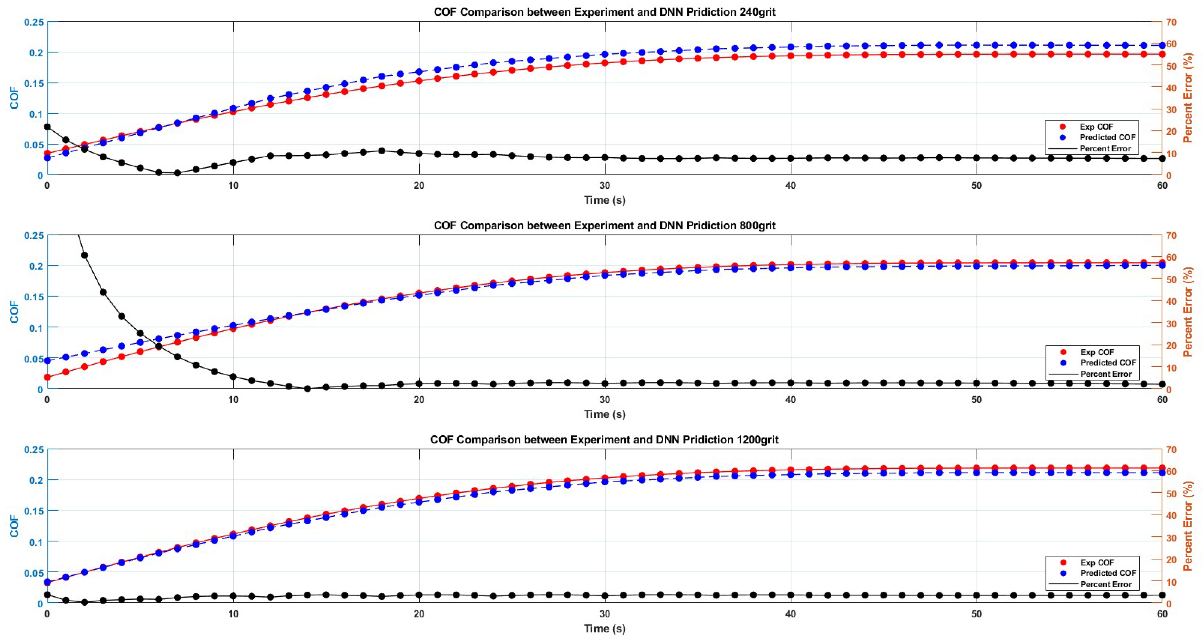
3.2. Coefficient of Friction

The experimental COF over a 60-second sliding period for the pin samples, derived from five replicates, is presented in Figure 4, where the solid line represents the average value and the shaded band indicates the error range. As the experiment was conducted five times under identical conditions, four sets were used to train the DNN model, with the COF as the output, while the remaining set was used to validate the predicted COF from the DNN. For all samples, the COF rises sharply within the first 10 s, increases more gradually from 10 to 40 s, and stabilizes between 0.18 and 0.25 after 40 s. The 240-grit sample exhibits a slightly higher COF in the later stages, while the 800-grit sample displays a marginally lower COF, and the 1200-grit sample is intermediate. Smoother surfaces typically have larger real contact areas because there are fewer irregularities to interrupt contact between the sliding surfaces [40,41]. This increased contact can enhance the interfacial adhesion between the surfaces, which may result in a higher COF [42]. Furthermore, the interlocking of asperities on contacting surfaces also enhances the COF. In the 800-grit sample, although an increased contact area enhances adhesion between the surfaces, reduced asperity interlocking decreases the COF, with the latter dominating, resulting in the 800-grit sample exhibiting the lowest COF. For the 1200-grit samples, however, asperity interlocking is further reduced, while the contact area increases further, leading to a higher COF compared to the 800-grit samples.

3.3. Noise Signal Analysis

3.3.1. Time-Domain Signal (First 1 s)

Figure 5 presents the time-domain noise signals recorded during the first second of the wear test. All samples display rapid oscillations, suggesting high-frequency components. The 1200-grit sample exhibits larger amplitude fluctuations compared to the more stable patterns of the 240- and 800-grit samples. This variability in the smoother 1200-grit sample may stem from a larger contact area, concentrating load on fewer asperities and enhance stick–slip events, a common source of frictional noise [43,44]. Conversely, the rougher 240- and 800-grit surfaces yield more consistent amplitudes.

3.3.2. Power Spectral Density (PSD) Analysis

To analyze the frequency-domain characteristics of five replicates over the 60 s duration, PSD was computed, as shown in Figure 5. All samples display a similar PSD, with the majority of peaks concentrated below 100 Hz and additional peaks observed at 2000 Hz, 3000 Hz, and 5300 Hz. These findings indicate that smoother initial surfaces did not significantly alter the frequency of friction noise.

3.3.3. Spectrogram Analysis

The spectrograms in Figure 5 provides a time-frequency perspective of the noise signals across the grit levels.

Low-Frequency Dominance: Acoustic energy is concentrated in the 0 to 1000 Hz range for all three conditions, indicating that low-frequency components dominate the signal. This may correspond to the fundamental frequency of the measured process, such as frictional noise.

Consistent 2000 Hz Band: A horizontal band around 2000 Hz appears consistently across all spectrograms. This could represent a characteristic frequency of the process (e.g., a resonance) or an artifact from the measurement system. Its presence across all grit levels suggests it is independent of surface roughness.

Effect of Grit Size: The spectrograms for 240-grit, 800-grit, and 1200-grit surfaces exhibit remarkable similarity. This indicates that the source or generation mechanism of the acoustic signal remains consistent (thus resulting in a comparable frequency pattern), but the intensity or certain physical properties of the signal (e.g., friction or wear level) varies. It can be inferred that initial surface roughness influences the intensity of friction noise through modifications in the COF and surface morphology during the sliding process, yet it exerts minimal influence on the spectral peaks associated with specific physical processes (e.g., vibrational modes during friction or resonance frequencies).

Temporal Stability: The absence of significant temporal variations in the spectrograms indicates that the process remains stable over the 60 s duration, with no notable changes in operating conditions or signal characteristics.

3.3.4. One-Third Octave Band Analysis

Figure 6 provides a detailed comparison of the one-third octave band analysis for three different sandpaper grits, covering a frequency spectrum from 20 Hz to 8000 Hz. This analysis offers valuable insights into the primary noise sources generated during the sanding process, with the data clearly indicating that the dominant noise frequencies for all samples are centered at 50 Hz, 80 Hz, 250 Hz, and 630 Hz. These frequencies are likely associated with distinct mechanical or operational characteristics of the frictional sliding process. Specifically, the mid-range frequencies from 50 Hz to 250 Hz may indicate vibrations or resonances generated by the machinery or the wear process itself. Meanwhile, the higher frequency peak at 630 Hz may originate from rapid, high-energy interactions between the pin and the disc, potentially influenced by aerodynamic factors. Notably, these noise sources remain consistent across the three conditions, suggesting that they are fundamental to the frictional sliding process rather than being solely determined by surface roughness.

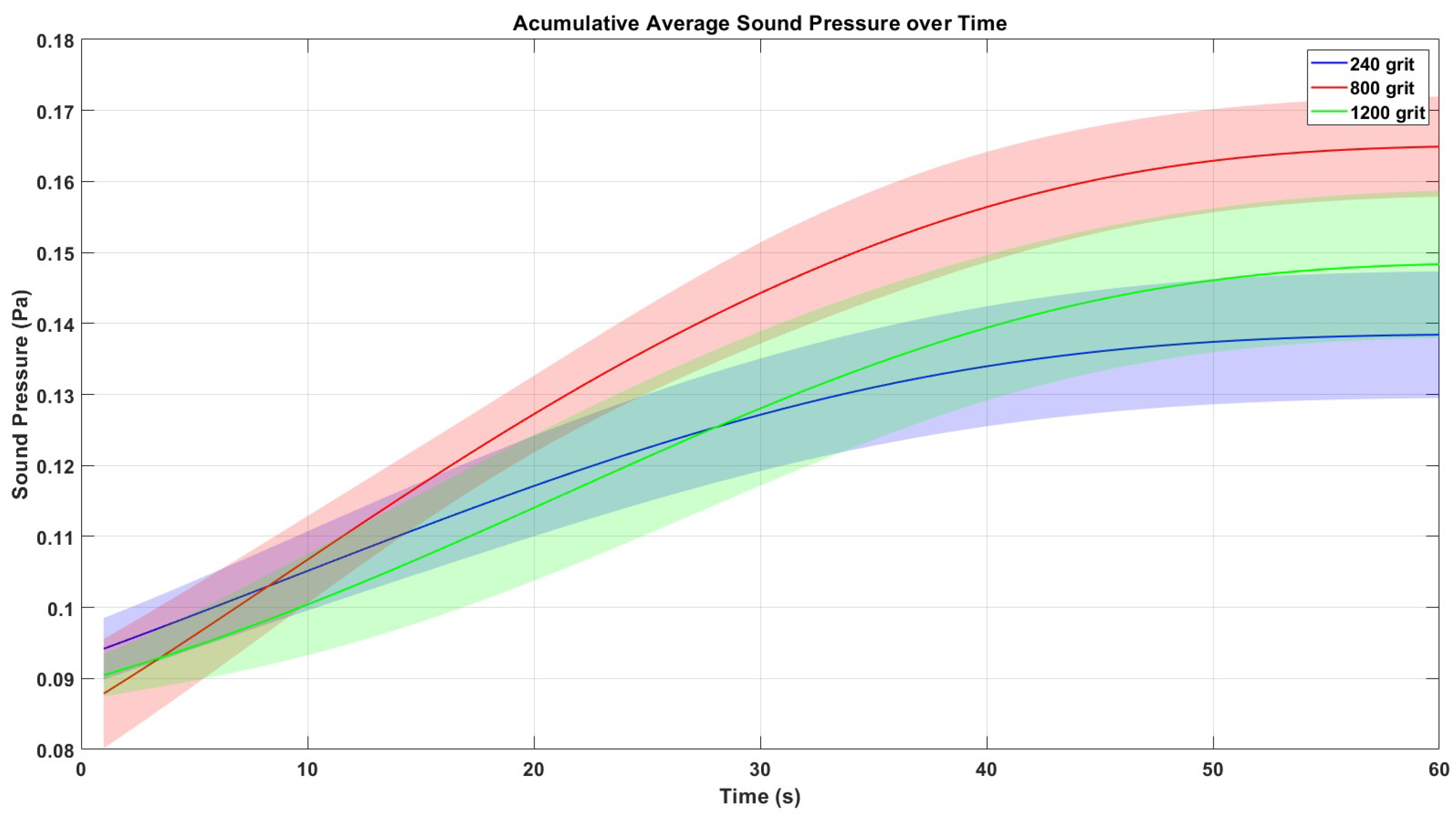
3.3.5. Accumulative Average Sound Pressure

Previous frequency-domain analyses cannot be directly employed as indicators to assess human perception in a noisy experiment, and pronounced nonlinearity renders it challenging to integrate frequency-domain noise signals into a DNN to predict the dynamic changes in wear morphology and COF during the frictional sliding process [45]. Consequently, the accumulative average sound pressure over the sliding duration under various conditions was analyzed, which reflects the average noise level over this period, as depicted in Figure 7. Accumulative average sound pressure (AASP) is more suitable than principal component analysis (PCA) and Mel-frequency cepstral coefficients (MFCC) for training a DNN to predict the COF and wear development because it operates in the time domain, aligning directly with the time-varying nature of the target variables. Unlike PCA, which is less effective for one-dimensional time-series data and introduces complexity in correlating extracted patterns with COF and wear, AASP offers a straightforward correlation. Compared to MFCC, which transforms signals into frequency-domain features, AASP avoids unnecessary transformations, making it more convenient for DNN training. Despite sacrificing some time-frequency details, AASP’s simplicity and directness make it the preferred choice for this task. The samples polished with 800-grit sandpaper exhibit the highest accumulative sound pressure (0.16 Pa), followed by those polished with 1200-grit sandpaper (0.15 Pa), while the 240-grit samples yield the lowest sound pressure (0.14 Pa). This result is unexpected, as previous research indicates that smoother surfaces often generate higher frictional forces during the “stick” phase, which, upon sudden release, may produce audible noise. This phenomenon is especially pronounced in dry sliding conditions, where the absence of lubrication fails to mitigate vibrations [46]. Nevertheless, although samples polished with 800-grit sandpaper exhibit a higher noise level than those polished with 240-grit sandpaper, further smoothing with 1200-grit sandpaper did not increase the noise level. This indicates that the relationship between noise and surface roughness may be more complex than merely attributing the noise level to stick–slip behavior during sliding. Investigating this relationship may require the consideration of how initial roughness affects changes in contact stiffness during wear development and how these changes contribute to the stability and vibration of the specific system, which lies beyond the scope of this study.

3.4. Mesh-Independent Validation and Deep Neural Network Training

To ensure the accuracy of the FEM model, mesh-independent validation was performed to confirm that simulation results exhibit minimal variation with mesh size refinement. The 1200-grit parameter was employed for the mesh-independent validation. In detail, the mesh size at the contact region was iteratively halved until the wear simulation results showed negligible changes, as shown in Figure 8. Despite further refinement of the mesh in the contact area, the wear simulation results remain nearly identical, indicating that the current mesh configuration is sufficiently reliable while maintaining reduced computational costs.

Figure 9 illustrates the variation in loss values during the training process of a deep neural network with increasing training iterations. The green line denotes the training loss, and the blue line denotes the validation loss. Both curves exhibit a consistent downward trend in loss values with increasing training epochs. During the initial training phase (approximately 0–200 epochs), the loss values decrease rapidly; subsequently, the rate of decrease gradually diminishes, stabilizing at approximately 0.002. The blue validation loss curve exhibits greater fluctuations than the green training loss curve, which is expected, as performance on the validation set is typically less stable than on the training set. Nevertheless, both curves ultimately converge to comparable values, suggesting that the model exhibits minimal overfitting or underfitting. Such loss curves suggest that the neural network training process is stable and has achieved successful convergence.

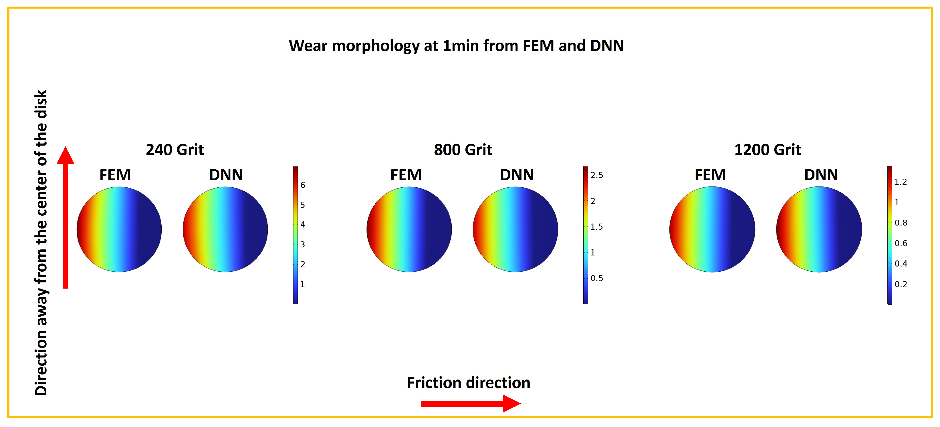
3.5. Wear and COF Prediction

The FEM model was validated against physical experiments to confirm that the predicted wear accurately matches experimental results. Subsequently, the wear depth distribution on the surface, obtained from the FEM model, was used to train the DNN. The worn surface profiles of experimental samples and the wear depths predicted by the finite element method (FEM) and DNN models were measured and extracted by tracing the red lines in Figure 10. Figure 11 presents a comparison of worn surface profiles under various conditions, which demonstrates that wear depth decreases with a smoother initial surface: the 240-grit-polished sample exhibits the deepest wear (up to $-6$ $\mathrm{\mu }$$\mathrm{m}$), the intermediate 800-grit-polished sample yields moderate wear (up to $-1.5$ $\mathrm{\mu }$$\mathrm{m}$), and the finest 1200-grit-polished surface displays the shallowest wear (limited to $-1$ $\mathrm{\mu }$$\mathrm{m}$). The FEM simulations closely align with the experimental results, validating the model’s reliability. Consequently, the results of the FEM model can be utilized to train the DNN model, with only minor differences between FEM and DNN outcomes on the validating dataset, indicating that the DNN can effectively substitute for FEM predictions of wear development. For example, using the 60 s accumulative average noise from the validation dataset, the DNN accurately predicts wear morphology consistent with the FEM (see Figure 12).

In Figure 11, the wear depths predicted by both the FEM and the DNN diverge from the experimental results. The mean wear depth values from DNN, FEM, and experimental data were calculated, followed by the computation of mean relative errors (MREs) of no more than 16%. This discrepancy arises because FEM simulations overlook the real surface roughness and the effects of wear debris. Incorporating these factors—namely, the rough surface and the wear debris generated during the sliding process—into FEM simulations is highly challenging. Such integration often results in convergence difficulties and renders the simulations computationally infeasible, as noted in [47]. By design, FEM adheres to physical laws, ensuring that its predictions align with fundamental physical principles. In contrast, the DNN employed in this study does not inherently uphold these constraints. Instead, it relies on numerical approximations introduced through its training process, optimization algorithms, and activation functions to mimic the FEM outcomes. As a result, differences persist between the wear depths predicted by FEM, DNN, and those observed in the experimental results.

Figure 13 compares the DNN-predicted COF with experimental values over the sliding duration. The predictions, based on noise signals from the validating dataset, align closely with experimental data, with relative errors below 10%, demonstrating the DNN’s accuracy in COF prediction.

To reduce the dataset size, we sampled the COF and noise signals every 6 s (from 0 to 60 s) during the experiment to train the DNN model. Although this coarse time sampling may introduce discrepancies with the experimental data, the DNN-predicted COFs in unseen scenarios (outside the selected time points) still closely align with the experimental results.

3.6. Strengths and Limitations of the Proposed Approach

The innovation of this method lies in the integration of both finite element method (FEM) and experimental approaches. By using FEM-derived wear results to replace experimental data for training the DNN, this approach significantly reduces experimental costs. Once the FEM model is validated against experimental wear data within a 1-min duration, it demonstrates alignment with experimental results. Consequently, FEM wear data at intervals of 0.1 min, 0.2 min, and beyond can be used to train the DNN, eliminating the need to conduct experiments at these time points. Furthermore, incorporating time-series COF and accumulative average sound pressure (AASP) data from experiments into DNN training enables the model to predict wear morphology and COF based on acoustic signals. A limitation of the proposed method’s accuracy is its reliance on the quality of datasets from both experiments and FEM, as these datasets are derived from specific materials under a defined range of experimental parameter configurations. Beyond this range, the DNN may fail to provide reliable predictions.

4. Conclusions

Friction noise primarily stems from asperity collisions, mode coupling, and stick–slip transitions at the sliding interface. The friction force induces structural vibrations, which, through normal-direction motion of the surface, generate air vibrations that radiate as sound. Wear alters the contact interface, modifying friction characteristics and contact stiffness, thereby affecting the vibration system. The nonlinear interactions among friction, wear, and vibration during sliding complicate the development of analytical models or numerical simulations to study their relationships.

Therefore, this study develops a DNN model to predict wear patterns and the COF during frictional sliding. To do this, we combined experimental testing with finite element method (FEM) simulations to create a strong dataset for training the DNN.

We tested brass pins (UNS C38500), polished to different roughness levels using 240-, 800-, and 1200-grit sandpaper, sliding against a 304 stainless steel disc under controlled conditions. These experiments provided data to check the FEM model, which accurately simulated how wear changes over time. The close match between experimental and simulated worn surface profiles confirmed the FEM’s reliability.

We trained the DNN model using validated FEM wear simulations and inputs like acoustic signals, wear coefficients, and time-related data. When given frictional noise as input, the DNN predicted a COF with less than 10% error compared to experimental results. It also matched FEM wear depth simulations well, offering a faster alternative to traditional FEM methods.

Although this approach was developed using a brass–steel pin-on-disc frictional pair, it could be further extended to other industrial machinery or frictional pairs composed of diverse materials to monitor and predict wear and friction in real time using acoustic signals.

References

1. Meng, Y.; Xu, J.; Ma, L.; Jin, Z.; Prakash, B.; Ma, T.; Wang, W. A review of advances in tribology in 2020–2021. Friction 2022, 10, 1443–1595. [Google Scholar]
2. Erdemir, A.; Ramirez, G.; Eryilmaz, O.; Narayanan, B.; Liao, Y.; Kamath, G.; Sankaranarayanan, S.K.R.S. Carbon-based tribofilms from lubricating oils. Nature 2016, 536, 67–71. [Google Scholar] [CrossRef] [PubMed]
3. Tomanik, E.; Christinelli, W.; Souza, R.M.; Oliveira, V.L.; Ferreira, F.; Zhmud, B. Review of Graphene-Based Materials for Tribological Engineering Applications. Eng 2023, 4, 2764–2811. [Google Scholar] [CrossRef]
4. Kasar, A.K.; Menezes, P.L. Synthesis and recent advances in tribological applications of graphene. Int. J. Adv. Manuf. Technol. 2018, 97, 3999–4019. [Google Scholar] [CrossRef]
5. Che, Q.; Zhang, G.; Zhang, L.; Qi, H.; Li, G.; Zhang, C.; Guo, F. Switching brake materials to extremely wear-resistant self-lubrication materials via tuning interface nanostructures. ACS Appl. Mater. Interfaces 2018, 10, 19173–19181. [Google Scholar] [CrossRef]
6. Wong, V.W.; Tung, S.C. Overview of automotive engine friction and reduction trends–Effects of surface, material, and lubricant-additive technologies. Friction 2016, 4, 1–28. [Google Scholar] [CrossRef]
7. Dwyer-Joyce, R.; Rahnejat, H. Special Issue on Automotive Piston–Cylinder Tribology. Proc. Inst. Mech. Eng. Part J. Eng. Tribol. 2013, 227, 99. [Google Scholar] [CrossRef]
8. Miyoshi, K. Aerospace mechanisms and tribology technology: Case study. Tribol. Int. 1999, 32, 673–685. [Google Scholar] [CrossRef]
9. Voevodin, A.A.; O’Neill, J.P.; Zabinski, J.S. Nanocomposite tribological coatings for aerospace applications. Surf. Coatings Technol. 1999, 116, 36–45. [Google Scholar] [CrossRef]
10. Ralls, A.M.; Kumar, P.; Menezes, P.L. Tribological properties of additive manufactured materials for energy applications: A review. Processes 2020, 9, 31. [Google Scholar] [CrossRef]
11. Schmid, S.R.; Saha, P.K.; Wang, J.; Schmitz, T. Developments in tribology of manufacturing processes. J. Manuf. Sci. Eng. 2020, 142, 110803. [Google Scholar] [CrossRef]
12. Feng, P.; Borghesani, P.; Smith, W.A.; Randall, R.B.; Peng, Z. A review on the relationships between acoustic emission, friction and wear in mechanical systems. Appl. Mech. Rev. 2020, 72, 020801. [Google Scholar] [CrossRef]
13. Tian, Y.; Khan, M.; Yuan, H.; Zheng, B. Wear modeling and friction-induced noise: A review. Friction 2025, 9441124. [Google Scholar] [CrossRef]
14. Meng, M.; Wang, X.S.; Li, K.Y.; Deng, Z.X.; Zhang, Z.Z.; Sun, Y.L.; Zhang, S.F.; He, L.; Guo, J.W. Effects of surface roughness on the time-dependent wear performance of lithium disilicate glass ceramic for dental applications. J. Mech. Behav. Biomed. Mater. 2021, 121, 104638. [Google Scholar] [CrossRef]
15. Zurek, A.D.; Alfaro, M.F.; Wee, A.G.; Yuan, J.C.-C.; Barao, V.A.; Mathew, M.T.; Sukotjo, C. Wear characteristics and volume loss of CAD/CAM ceramic materials. J. Prosthodont. 2019, 28, e510–e518. [Google Scholar] [CrossRef]
16. Ghosh, G.; Sidpara, A.; Bandyopadhyay, P.P. Understanding the role of surface roughness on the tribological performance and corrosion resistance of WC-Co coating. Surf. Coatings Technol. 2019, 378, 125080. [Google Scholar] [CrossRef]
17. Briggs, G.A.D.; Briscoe, B.J. Effect of surface roughness on rolling friction and adhesion between elastic solids. Nature 1976, 260, 313–315. [Google Scholar] [CrossRef]
18. Zhou, B.; Ma, J.; Yang, Z.; Shi, X. Noise reduction mechanism and analysis of TC4 with dimple textured surfaces. J. Mater. Eng. Perform. 2021, 30, 3859–3871. [Google Scholar] [CrossRef]
19. Gurumoorthy, S.; Bhimchand, N.; Bourgeau, A.; Bhumireddy, Y. Effect of Surface Roughness on Tribological and NVH Behaviour of Brake System. In SAE Technical Paper; SAE International: Warrendale, PA, USA, 2024; p. 2024-01-2732. [Google Scholar]
20. Sose, A.T.; Joshi, S.Y.; Kunche, L.K.; Wang, F.; Deshmukh, S.A. A review of recent advances and applications of machine learning in tribology. Phys. Chem. Chem. Phys. 2023, 25, 4408–4443. [Google Scholar] [CrossRef]
21. Hasan, M.S.; Nosonovsky, M. Triboinformatics: Machine learning algorithms and data topology methods for tribology. Surf. Innov. 2022, 10, 229–242. [Google Scholar] [CrossRef]
22. Rosenkranz, A.; Marian, M.; Profito, F.J.; Aragon, N.; Shah, R. The use of artificial intelligence in tribology—A perspective. Lubricants 2020, 9, 2. [Google Scholar] [CrossRef]
23. Cheng, K.; Luo, X.; Ward, R.; Holt, R. Modeling and simulation of the tool wear in nanometric cutting. Wear 2003, 255, 1427–1432. [Google Scholar] [CrossRef]
24. Shah, R.; Pai, N.; Thomas, G.; Jha, S.; Mittal, V.; Shirvni, K.; Liang, H. Machine learning in wear prediction. J. Tribol. 2025, 147, 040801. [Google Scholar] [CrossRef]
25. Gouarir, A.; Martínez-Arellano, G.; Terrazas, G.; Benardos, P.; Ratchev, S.J.P.C. In-process tool wear prediction system based on machine learning techniques and force analysis. Procedia CIRP 2018, 77, 501–504. [Google Scholar] [CrossRef]
26. Rajput, A.S.; Das, S. A machine learning approach to predict the wear behaviour of steels. Tribol. Int. 2023, 185, 108500. [Google Scholar] [CrossRef]
27. Molinari, J.-F.; Aghababaei, R.; Brink, T.; Frérot, L.; Milanese, E. Adhesive wear mechanisms uncovered by atomistic simulations. Friction 2018, 6, 245–259. [Google Scholar] [CrossRef]
28. Han, Y.; Zhang, D.; Sun, Q.; Qin, J.; Chen, L.; Qian, L.; Wang, Y. Atomic-scale wear behaviors of iron oxide through the atom-by-atom attrition and plastic deformation of nano-asperities. Tribol. Int. 2023, 188, 108878. [Google Scholar] [CrossRef]
29. Gnecco, E.; Bennewitz, R.; Pfeiffer, O.; Socoliuc, A.; Meyer, E. Friction and wear on the atomic scale. In Springer Handbook of Nanotechnology; Springer: Berlin/Heidelberg, Germany, 2010; pp. 923–953. [Google Scholar]
30. Abdelounis, H.B.; Zahouani, H.; Le Bot, A.; Perret-Liaudet, J.; Tkaya, M.B. Numerical simulation of friction noise. Wear 2011, 271, 621–624. [Google Scholar] [CrossRef]
31. Lontin, K.; Khan, M.A. Wear and airborne noise interdependency at asperitical level: Analytical modelling and experimental validation. Materials 2021, 14, 7308. [Google Scholar] [CrossRef]
32. Basit, K.; Shams, H.; Khan, M.A.; Mansoor, A. Vibration analysis approach to model incremental wear and associated sound in multi-contact sliding friction mechanisms. J. Tribol. 2023, 145, 091201. [Google Scholar] [CrossRef]
33. Basit, K.; Shams, H.; Khan, M.A.; Mansoor, A. Empirical modelling of frictional noise and two-point contact using ball-on-disc tribometer. In Proceedings of the TESConf 2020—9th International Conference on Through-life Engineering Services, Cranfield, UK, 3–4 November 2020; p. 3717985. [Google Scholar]
34. Tian, Y.; Khan, M.; Deng, H.; Omar, I. Quantifying the interrelationship between friction, wear, and noise: A comparative study on aluminum, brass, and steel. Tribol. Int. 2025, 203, 110403. [Google Scholar] [CrossRef]
35. Huang, Z.; Zhu, J.; Lei, J.; Li, X.; Tian, F. Tool wear predicting based on multi-domain feature fusion by deep convolutional neural network in milling operations. J. Intell. Manuf. 2020, 31, 953–966. [Google Scholar] [CrossRef]
36. Cai, W.; Zhang, W.; Hu, X.; Liu, Y. A hybrid information model based on long short-term memory network for tool condition monitoring. J. Intell. Manuf. 2020, 31, 1497–1510. [Google Scholar] [CrossRef]
37. Sun, H.; Zhang, J.; Mo, R.; Zhang, X. In-process tool condition forecasting based on a deep learning method. Robot. Comput.-Integr. Manuf. 2020, 64, 101924. [Google Scholar] [CrossRef]
38. Xu, X.; Wang, J.; Zhong, B.; Ming, W.; Chen, M. Deep learning-based tool wear prediction and its application for machining process using multi-scale feature fusion and channel attention mechanism. Measurement 2021, 177, 109254. [Google Scholar] [CrossRef]
39. He, Z.; Shi, T.; Xuan, J.; Li, T. Research on tool wear prediction based on temperature signals and deep learning. Wear 2021, 478, 203902. [Google Scholar] [CrossRef]
40. Néder, Z.; Váradi, K. Contact behaviour of the original and substituted real surfaces. Int. J. Mach. Tools Manuf. 2001, 41, 1935–1939. [Google Scholar] [CrossRef]
41. Quaglini, V.; Dubini, P. Friction of polymers sliding on smooth surfaces. Adv. Tribol. 2011, 2011, 178943. [Google Scholar] [CrossRef]
42. Hsia, F.-C.; Franklin, S.; Audebert, P.; Brouwer, A.M.; Bonn, D.; Weber, B. Rougher is more slippery: How adhesive friction decreases with increasing surface roughness due to the suppression of capillary adhesion. Phys. Rev. Res. 2021, 3, 043204. [Google Scholar] [CrossRef]
43. Le Bot, A. Noise of sliding rough contact. In Journal of Physics: Conference Series; IOP Publishing: Bristol, UK, 2017; Volume 797, p. 012006. [Google Scholar]
44. Yang, C.; Persson, B.N.J. Contact mechanics: Contact area and interfacial separation from small contact to full contact. J. Phys. Condens. Matter 2008, 20, 215214. [Google Scholar] [CrossRef]
45. Colbrook, M.J.; Antun, V.; Hansen, A.C. The difficulty of computing stable and accurate neural networks: On the barriers of deep learning and Smale’s 18th problem. Proc. Natl. Acad. Sci. USA 2022, 119, e2107151119. [Google Scholar] [CrossRef] [PubMed]
46. Lontin, K.; Khan, M. Interdependence of friction, wear, and noise: A review. Friction 2021, 9, 1319–1345. [Google Scholar] [CrossRef]
47. Tian, Y.; Zheng, B.; Khan, M.; He, F. Influence of sliding direction relative to layer orientation on tribological performance, noise, and stability in 3D-printed ABS components. Tribol. Int. 2025, 210, 110762. [Google Scholar] [CrossRef]
Figure 1. Experiment dimension.
Processes 13 01762 g001
Figure 2. (a) Wear experiment setup, (b) Worn surface profile measurement, (c) FEM mesh.
Processes 13 01762 g002
Figure 3. DNN framework.
Processes 13 01762 g003
Figure 4. COF over time for samples with different initial roughness levels.
Processes 13 01762 g004
Figure 5. Detailed analysis of signal characteristics for 240-grit, 800-grit, and 1200-grit surfaces using time-domain (first 1−s window), frequency-domain, and time-frequency-domain visualizations, illustrating variations in amplitude, frequency content, and temporal evolution across surface roughness levels.
Processes 13 01762 g005
Figure 6. One-third band analysis for 240-grit, 800-grit, and 1200-grit surfaces.
Processes 13 01762 g006
Figure 7. Cumulative average sound pressure over sliding duration under 240-grit, 800-grit, and 1200-grit surfaces (shadow bands indicates standard deviations).
Processes 13 01762 g007
Figure 8. Mesh-independent validation.
Processes 13 01762 g008
Figure 9. Deep neural network training: convergence of training and validation loss over 1500 epochs.
Processes 13 01762 g009
Figure 10. Worn surface profile measurement.
Processes 13 01762 g010
Figure 11. Worn surface profiles of samples: comparison of experimental, FEM, and DNN results.
Processes 13 01762 g011
Figure 12. Worn surface under different conditions at 1 min from DNN and FEM.
Processes 13 01762 g012
Figure 13. Comparison between experimental and predicted COFs over 60 s.
Processes 13 01762 g013