Abstract
In the aluminum electrolysis production process, the traditional cell control method based on cell voltage and series current can no longer meet the goals of energy conservation, consumption reduction, and digital-intelligent transformation. Therefore, a new digital cell control technology that is centrally dependent on various process parameters has become an urgent demand in the aluminum electrolysis industry. Among them, the real-time online measurement of alumina concentration is one of the key data points for implementing such technology. However, due to the harsh production environment and limitations of current sensor technologies, hardware-based detection of alumina concentration is difficult to achieve. To address this issue, this study proposes a soft-sensing model for alumina concentration based on a long short-term memory (LSTM) neural network optimized by a weighted average algorithm (WAA). The proposed method outperforms BiLSTM, CNN-LSTM, CNN-BiLSTM, CNN-LSTM-Attention, and CNN-BiLSTM-Attention models in terms of predictive accuracy. In comparison to LSTM models optimized using the Grey Wolf Optimizer (GWO), Harris Hawks Optimization (HHO), Optuna, Tornado Optimization Algorithm (TOC), and Whale Migration Algorithm (WMA), the WAA-enhanced LSTM model consistently achieves significantly better performance. This superiority is evidenced by lower MAE and RMSE values, along with higher R2 and accuracy scores. The WAA-LSTM model remains stable throughout the training process and achieves the lowest final loss, further confirming the accuracy and superiority of the proposed approach.
1. Introduction
In industrial process control, some important process values—like reactant amount and phase change points—have a big effect on product quality. But because online detection tools are not fully developed and sensors are expensive, it is often not possible to watch these values in real time. To address this, the engineering community has proposed soft-sensing technology, which constructs mathematical models linking measurable process variables like temperature, pressure, and flow rate with target parameters, thereby enabling indirect dynamic estimation based on measurable variables. In such cases, mathematical models developed using easily measurable variables to monitor hard-to-measure variables are referred to as soft-sensing models. In the aluminum electrolysis production process, low and locally uneven alumina concentrations can cause spikes and other deformations at the anode bottom [1,2,3].
Conversely, excessively high alumina concentration slows the dissolution rate of alumina, leading to the formation of insoluble sludge that erodes the cathode. Therefore, the alumina concentration should be maintained within a certain range and evenly distributed [4]. Practice shows that the mass fraction of alumina in the aluminum electrolysis cell should be controlled within a narrow range of 1.5% to 3.5%. Outside this range, common accidents such as anode effect, cell leakage, electrolyte splashing, and “rolling aluminum” can occur. When the concentration drops below 1.5%, the electrolysis system faces critical risks: frequent anode effects, electrolyte–aluminum interface tension imbalance triggering “rolling aluminum,” and excessively reduced electrolyte viscosity causing leakage accidents. Conversely, when the concentration exceeds 3.5%, sudden changes in the viscosity of the liquid electrolyte cause electrolyte splashing [5]. Therefore, achieving high efficiency, stability, and energy economy in aluminum electrolysis production requires precise prediction and dynamic control of alumina concentration as the technical foundation.
Remark 1.

Given the large number of abbreviations used throughout the manuscript, an abbreviation list is provided here to facilitate readability of the subsequent sections as shown in Table 1.
Table 1.
Terms and Their Corresponding Abbreviations.
In industrial process control for aluminum electrolysis, alumina concentration is a key process indicator, and its real-time monitoring has long been a technical bottleneck for the industry. Consequently, international investigators have continuously explored online measurement and prediction methods, yielding several important research achievements. Gen et al. [6] established a simulation model of alumina concentration based on a Particle Swarm Optimization (PSO)-optimized Back Propagation Neural Network (BP neural network) prediction model. Zhu et al. [7] used a PSO-LSTM neural network-improved model to predict the changing trend of alumina concentration in aluminum electrolysis cells. Du et al. [8] performed dynamic simulation of alumina concentration based on real-time anode current signals and future predicted values combined with dynamic U-shaped curve relationships, supported by an offline Computational Fluid Dynamics (CFD) simulation database of alumina concentrations. Cao et al. [9] employed an improved quantum genetic algorithm to optimize a BP neural network model for alumina concentration prediction in aluminum electrolysis cells. Li et al. [10] proposed a Soft Deep Belief Network (SDBN) model based on co-training, called Co-reg SDBN, for soft sensing. Ma et al. [11] used an H∞ filter to estimate alumina concentration in real time by utilizing alumina feed rate, beam movement, and voltage measurements. Ma et al. [12] developed a robust Kalman filter to estimate spatial alumina concentration using voltage measurements and single anode current data. Huang et al. [13] proposed a data-driven soft sensor prediction method for alumina concentration based on an Improved Genetic Algorithm (IGA) optimized Echo State Network (ESN).
Previous studies aiming to improve alumina concentration prediction accuracy proposed a hybrid modeling method based on Empirical Mode Decomposition (EMD), Particle Swarm Optimization (PSO), and Deep Belief Networks (DBN), known as EMD-PSO-DBN. In this method, raw data are denoised by empirical mode decomposition (EMD), and the deep belief network (DBN) structure is optimized by Particle Swarm Optimization (PSO) to improve soft sensing accuracy through signal denoising and parameter optimization [14]. Considering that DBN model parameters significantly impact prediction accuracy, an Improved Gray Wolf Optimizer (IGWO) was further proposed to optimize the DBN model. Simulation verified the method’s effectiveness and moderately improved prediction accuracy and stability [15].
To further enhance the precise prediction of alumina concentration in industrial aluminum electrolysis, this study employs long short-term memory (LSTM) networks for prediction. Prior to this, LSTM networks have been applied in various fields, such as link prediction in social networks [16], prediction of negative anode effects in aluminum electrolysis cells [17], molecular understanding and prediction [18], and river flow forecasting [19].
However, achieving good performance using LSTM networks is not a trivial task, as it involves optimizing multiple hyperparameters. Choosing the best parameters for neural network architectures often results in performance differences ranging from mediocre to state-of-the-art [20]. Existing literature shows that applying intelligent optimization algorithms to LSTM hyperparameter tuning has become an effective way to improve model performance, with a series of positive results. For example, Wang et al. [21] proposed a short-term water quality prediction model based on variational mode decomposition (VMD) and an Improved Grasshopper Optimization Algorithm (IGOA) to optimize the LSTM network. Li et al. [22] presented a building energy prediction method based on Bayesian optimization (BO) and spatiotemporal attention (STA) to enhance LSTM.
Currently, there are few bibliometric studies on trends in aluminum electrolysis research [23]. Although soft-sensing technology has been successfully applied to alumina concentration prediction in aluminum electrolysis, the incomplete theoretical framework and lack of practical guidance methods remain important bottlenecks limiting further development. To address practical application needs, this study builds a comparative research framework based on deep learning multi-models. The use of deep learning algorithms typically involves careful tuning of learning parameters and model hyperparameters [24]. By combining convolutional neural networks (CNNs), attention mechanisms, and LSTM networks in various configurations, the performance differences of multiple deep learning neural network models are examined. Moreover, comparative experiments involving multiple optimization algorithms are conducted to evaluate their performances, providing a basis for model selection in engineering practice.
This paper proposes an LSTM network optimized by the weighted average algorithm (WAA). The WAA optimizes the LSTM network’s neuron count, number of layers, learning rate, batch size, and number of iterations, forming the WAA-LSTM model. Experimental results indicate that this approach not only improves prediction accuracy and convergence speed but also enriches the theoretical foundation of alumina concentration soft sensing, offering significant guidance for practical applications. Simulation verification confirms its effectiveness in enhancing model stability and accuracy.
The remainder of this paper is organized as follows: Section 2 presents the proposed methodology, introducing the principles of LSTM, BiLSTM, CNN, attention mechanisms, and the WAA. Section 3 describes the acquisition and preprocessing of the alumina concentration dataset, the evaluation metrics, and the overall design of the soft-sensing model. Section 4 provides experimental analyses based on ensemble machine learning algorithms, including parameter optimization results and simulation comparisons for different models. Section 5 compares the simulation results of the WAA-LSTM model with those of other optimization algorithms. Section 6 performs statistical testing and analysis across the 12 models. Finally, Section 7 summarizes the principal experimental findings and outlines future research directions.
2. Prediction Models and Optimization Algorithm
2.1. Neural Network Model Architecture
2.1.1. Long Short-Term Memory Network (LSTM)
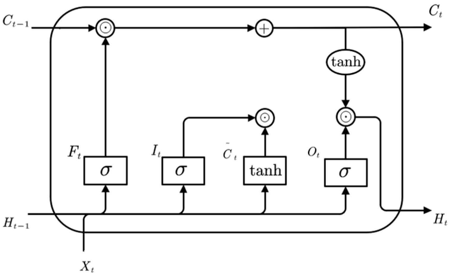
The LSTM is a specialized type of recurrent neural network designed to alleviate the vanishing gradient problem encountered in traditional recurrent neural networks (RNNs). By introducing gating mechanisms to control the flow of information, LSTM enables the model to better retain long-term dependencies and mitigate gradient vanishing [25,26]. The structure of the LSTM network is illustrated in Figure 1.
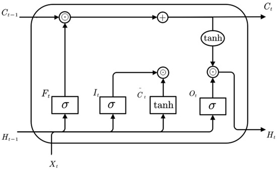
Figure 1.
Structure diagram of the LSTM network.
These gating units enable the LSTM to selectively retain or forget information and determine which data should be passed on to the next time step. The forget gate determines which information should be discarded. The calculation is shown in Equation (1):
In the equation, denotes the sigmoid activation function; is the forget gate; and are the weight matrices; and is the bias term.
The input gate controls which information flows into the current memory cell. The computation is shown in Equations (2)–(4):
In the equations, is the input gate; is the candidate memory cell state matrix; is the memory cell state; and are the weight matrices of the input gate; and are the weight matrices of the memory cell; and and are the bias terms for the input gate and memory cell, respectively.
The output gate determines which memory information flows into the hidden state. The memory cell serves as a specialized hidden state that retains historical information. It is formed by combining the candidate memory cell and the memory cell from the previous time step, and the flow of information from the memory cell to the hidden state is regulated by the output gate. The computation process is shown in Equations (5) and (6).
In the equation, is the output gate; and are the weight matrices; is the bias term; is the output of the hidden layer; and is the hyperbolic tangent activation function.
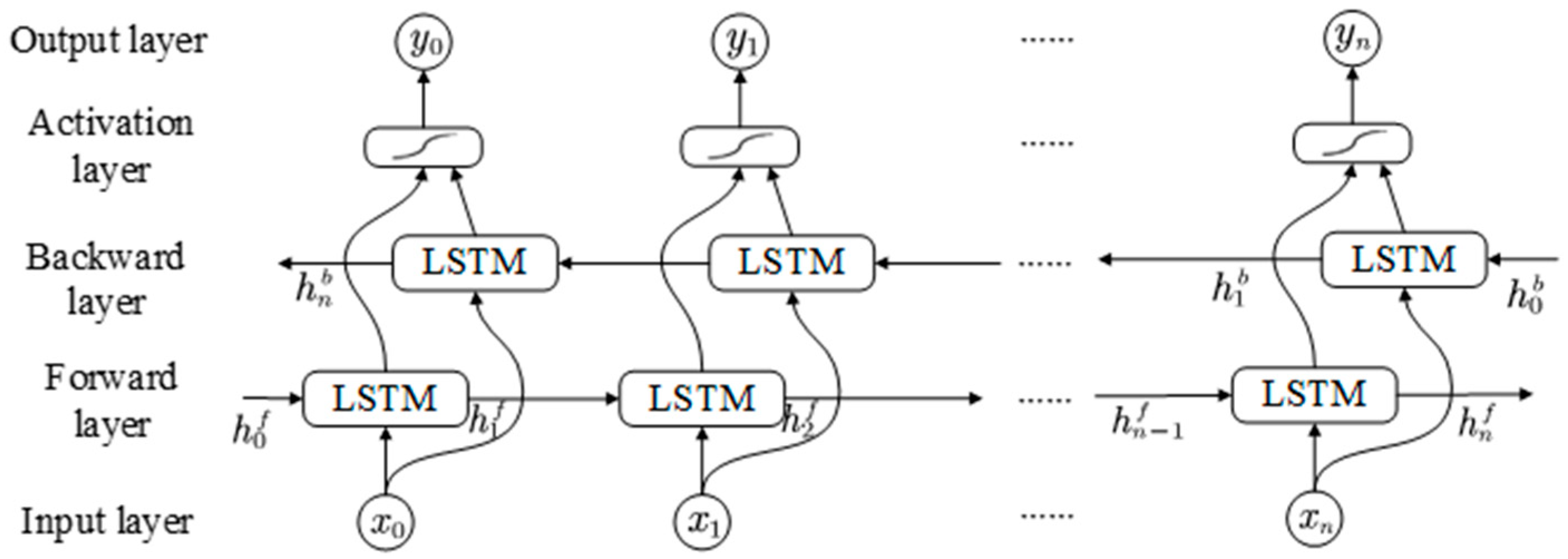
2.1.2. Bi-Directional Long Short-Term Memory Network (BiLSTM)
The BiLSTM network is an extension of the standard LSTM architecture that enables simultaneous learning of both forward and backward dependencies in sequential data. A BiLSTM consists of two independent LSTM layers: a forward LSTM that processes the input sequence from beginning to end, and a backward LSTM that processes the sequence in reverse [27]. The forward LSTM learns from past data, and the backward LSTM learns from future data by reading it backward. The outputs of the two LSTM layers are then joined together—by putting them side by side or using other simple methods—to make the final result. This design helps BiLSTM get more useful information at each time step, which makes the model work better. Figure 2 shows how the BiLSTM network is built.
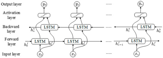
Figure 2.
Structure diagram of the BiLSTM network.
2.1.3. Convolutional Neural Network (CNN)
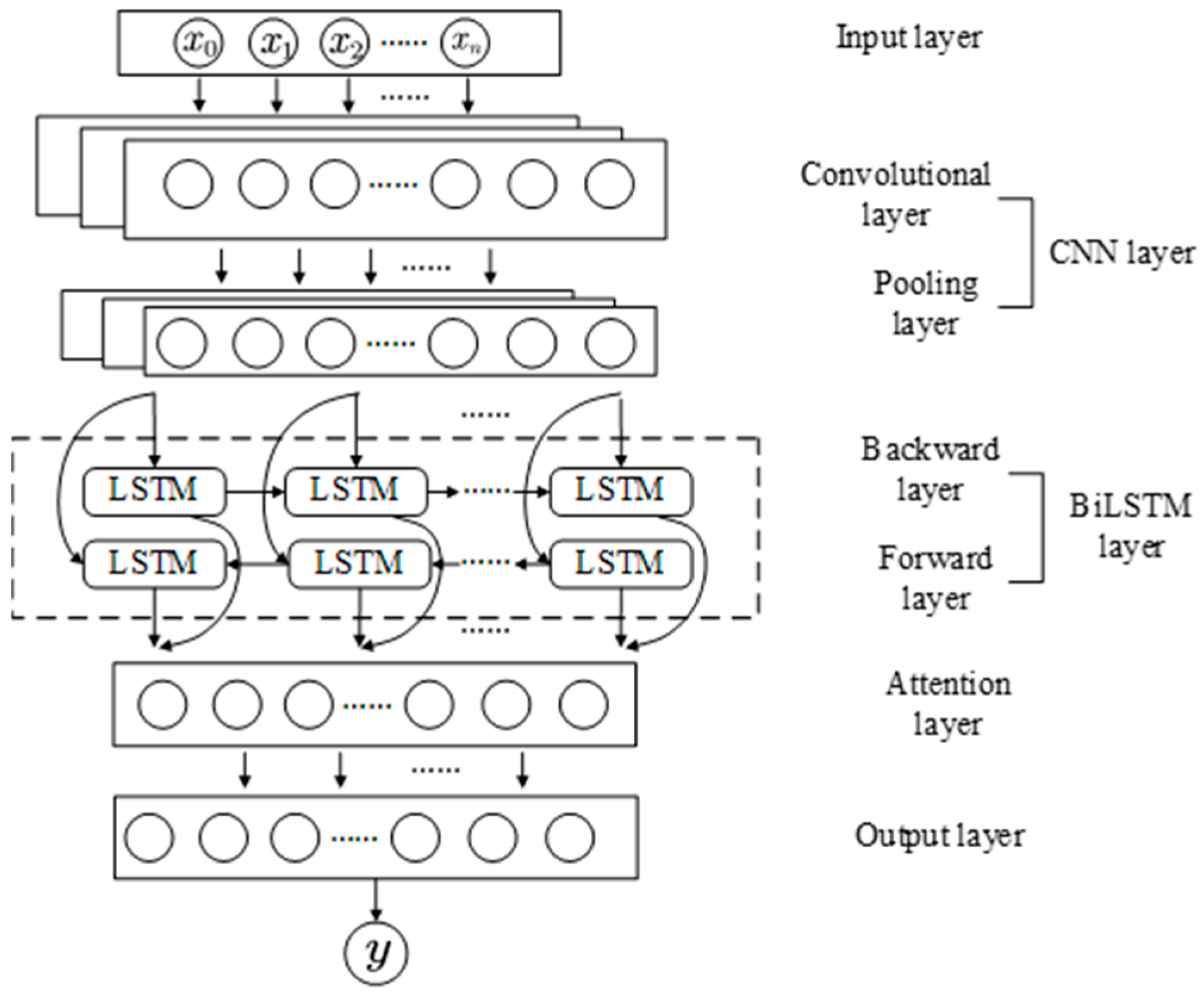
A convolutional neural network (CNN) consists of five main components: the input layer, convolutional layers, pooling layers, fully connected layers, and the output layer [28]. The convolutional layers perform efficient nonlinear feature extraction through local connections and weight-sharing mechanisms, making them particularly well-suited for pattern recognition in sequential data. The pooling layers compress and optimize the extracted features through down-sampling operations, thereby refining more discriminative and essential feature information.
2.1.4. Attention Mechanism
The attention mechanism was first introduced in the field of computer vision. Unlike traditional neural networks that treat all input signals uniformly, the attention mechanism dynamically evaluates the importance of features and assigns differentiated weights accordingly. By assigning higher weights to critical features and diminishing the influence of irrelevant information, this mechanism not only significantly enhances information processing efficiency but also effectively mitigates the issue of information degradation that LSTM networks face when dealing with long sequences [29]. Therefore, incorporating an attention mechanism may further improve prediction accuracy.
2.1.5. Composition of Hybrid Prediction Models
As mentioned earlier, accurately predicting alumina concentration is critically important for industrial production, prompting researchers to explore various methods for this purpose. There remains significant room for improving prediction accuracy, especially with advancements in technology. This paper proposes an alumina concentration prediction method based on the WAA-LSTM model and compares it with BiLSTM, CNN-LSTM, CNN-BiLSTM, CNN-LSTM-Attention, and CNN-BiLSTM-Attention models. Conv1D is used to process input data through convolution operations to extract local features; BiLSTM serializes these extracted local features, enabling the capture of both local characteristics and long-range dependencies within sequential data. The attention mechanism adaptively recalibrates channel-wise feature responses by learning the importance of each channel, enhancing the model’s sensitivity and focus on critical features [30]. The structure of the hybrid neural network model, specifically the CNN-BiLSTM-Attention network, is illustrated in Figure 3.
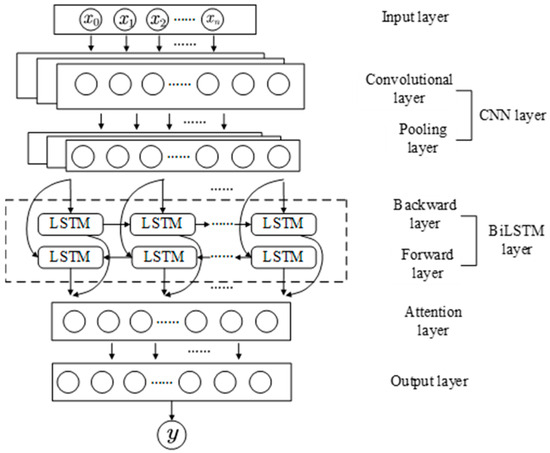
Figure 3.
Structure diagram of the CNN-BiLSTM-Attention network.
2.2. Weighted Average Algorithm (WAA)
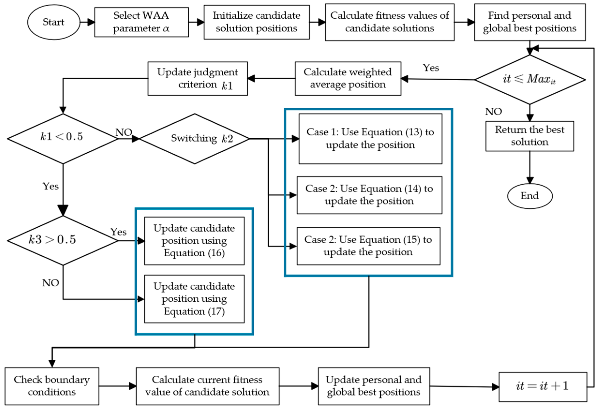
The weighted average algorithm (WAA) [31] was proposed by Jun Cheng and Wim De Waele in 2024. The concept of the weighted average position was directly introduced to develop this new metaheuristic optimization algorithm. The core idea of the WAA is to guide the optimization process using a weighted average position, where each candidate solution’s contribution is determined by its weight: the higher the weight, the stronger its influence on the final solution. As a statistical measure, the weighted average position reflects the importance of different elements through differentiated weights when calculating the overall mean, enabling the algorithm to more accurately balance global exploration and local exploitation capabilities.
The way the WAA works includes these main steps: First, in each round, the average position of all members is found using weights. Using this position, the algorithm moves in two steps to find the best solution. In the first step, the method combines the weighted average position with the best current solution, searching well by following three different directions. In the second step, the method uses the first step’s trend to quickly move toward the best solution and also uses a reverse trend to avoid getting stuck in bad spots. The selection of these movement strategies is dynamically regulated by a parameter function based on random constants and iteration counts, allowing the algorithm to adaptively balance exploration and exploitation as the search progresses. This unique balancing mechanism ensures the WAA’s outstanding performance in both global search capability and local optimization efficiency. The WAA initializes its population in a standard manner typical of intelligent optimization algorithms by randomly generating an initial solution set within the predefined search space. Its mathematical formulation is as follows:
Here, denotes a random number between 0 and 1; represents the lower bound of the -th variable for the given problem; and represents the upper bound of the -th variable for the given problem.
The first step in calculating the weighted average position is to evaluate the fitness value of each individual in the population and rank the individuals based on the nature of the optimization problem (maximization problem— or minimization problem—). Then, the top candidates are selected from the population to compute the weighted average position. The formula is as follows:
Here, denotes the total number of individuals in the population; represents the -th candidate solution; is the function used to calculate the fitness value; is the sum of the fitness values of the selected candidates; and is the weighted average position. Additionally, is the current iteration number, is the maximum number of iterations, and is the number of selected candidate solutions.
The WAA adaptively determines the search stage of candidate solutions through a dynamic parameter control mechanism. The stage selection formula is defined as follows:
Here, is the current iteration number, is the maximum number of iterations, and is a constant used to control the balance between exploration and exploitation phases. A fixed threshold of is employed to balance the algorithm’s exploration and exploitation behaviors: when the stage decision , candidate solutions enter the exploitation phase to perform a local fine-tuning search; when , they switch to the exploration phase for global search.
The first strategy in the exploitation phase uses the weighted average position, the individual best position, and the global best position to guide the search. It is expressed as follows:
Here, , , and are random values between 0 and 1, which are used to adjust the search space expansion around the individual best position and the global best position .
The second strategy guides the optimization process by constructing the search space between the weighted average position and the individual best position. Unlike the first strategy, this approach excludes the influence of the global best position, thereby narrowing the search scope. Its mathematical expression is as follows:
Here, and are random values between 0 and 1. This design enables the algorithm to focus more intensively on fine-tuning the search within potentially optimal regions.
The third strategy focuses on guiding the optimization process using the weighted average position and the global best position. The candidate solution update mechanism for this strategy can be expressed as follows:
Here, and are scalar values ranging from 0 to 1. This strategy’s search space is narrower compared to the first and second strategies. Moving from the global best position toward the weighted average position enhances both the convergence speed and accuracy.
The first exploration strategy during the exploration phase is defined as follows:
where represents the step size of the Lévy flight, denotes the -th position of the global best solution at iteration , and represents the -th position of the -th solution at iteration .
To address the potential issue where the algorithm may mistakenly identify a suboptimal solution as the global best, the WAA adopts a second movement strategy for optimization adjustment. When the first strategy faces the risk of local convergence due to the global best position deviating from the true optimal region, the second strategy reconstructs the search space by discarding the global best position and instead focusing on a combination of the weighted average position and the personal best position:
The variables and represent the minimum values of the lower and upper bounds across all dimensions, respectively. This design effectively prevents the misidentified global best position from misleading the search process into suboptimal regions. Meanwhile, by preserving the weighted average position, it maintains population diversity, and through incorporating individual best positions, it ensures the local search capability. This strategy dynamically balances exploration and exploitation, significantly enhancing the algorithm’s ability to escape local optima and ensuring better solutions in complex optimization problems. The algorithm flowchart is shown in Figure 4 [31].
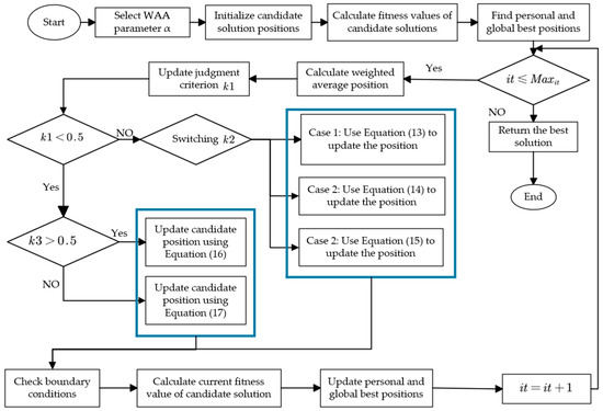
Figure 4.
WAA flowchart.
2.3. Selection of Model Parameters
In this study, the number of output channels in the convolutional layer is set to 64, with a kernel size of 3 and a stride of 1. The key hyperparameters of the LSTM model include the learning rate, training batch size, number of hidden units, and number of iterations. The learning rate affects model complexity and generalization ability, the batch size influences training speed and efficiency, the number of hidden units impacts the model’s representational capacity, and the number of iterations determines the degree of model fitting [32]. Therefore, the WAA optimization algorithm is employed to identify the optimal combination of hyperparameters. Five key hyperparameters are defined: the number of neurons, number of neural network layers, learning rate, batch size, and number of training epochs. A reasonable search space is set for each hyperparameter to cover potential optimal configurations, as shown in Table 2.
Table 2.
Hyperparameter search space ranges.
Given that this study involves a large number of combinations during hyperparameter optimization and that training each deep model (especially LSTM variants) is computationally intensive, increasing the number of cross-validation folds would prohibitively escalate computational cost. Under the current computational resource constraints, conducting repeated experiments is infeasible. Therefore, a three-fold cross-validation method is employed to evaluate the model performance. The dataset is divided into three subsets, each serving as the test set in turn, while the remaining subsets are used as training and validation sets. This procedure is repeated multiple times, with different subsets employed as the test set each time.
3. Experimental Simulation
3.1. Aluminum Electrolytic Data
This study focuses on the aluminum electrolysis production process at the Zunyi Aluminum Plant. The core process of modern aluminum electrolysis industrial production is realized through the electrochemical reactions at the electrodes of the electrolytic cell. Figure 5 [33] illustrates a schematic diagram of the typical structure of a modern aluminum electrolytic cell. The aluminum metal produced by the reduction reaction is deposited at the bottom of the electrolytic cell, while the oxygen generated during the process is released at the top of the cell, thereby completing the electrolysis process.
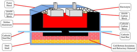
Figure 5.
Schematic diagram of the aluminum electrolytic cell structure.
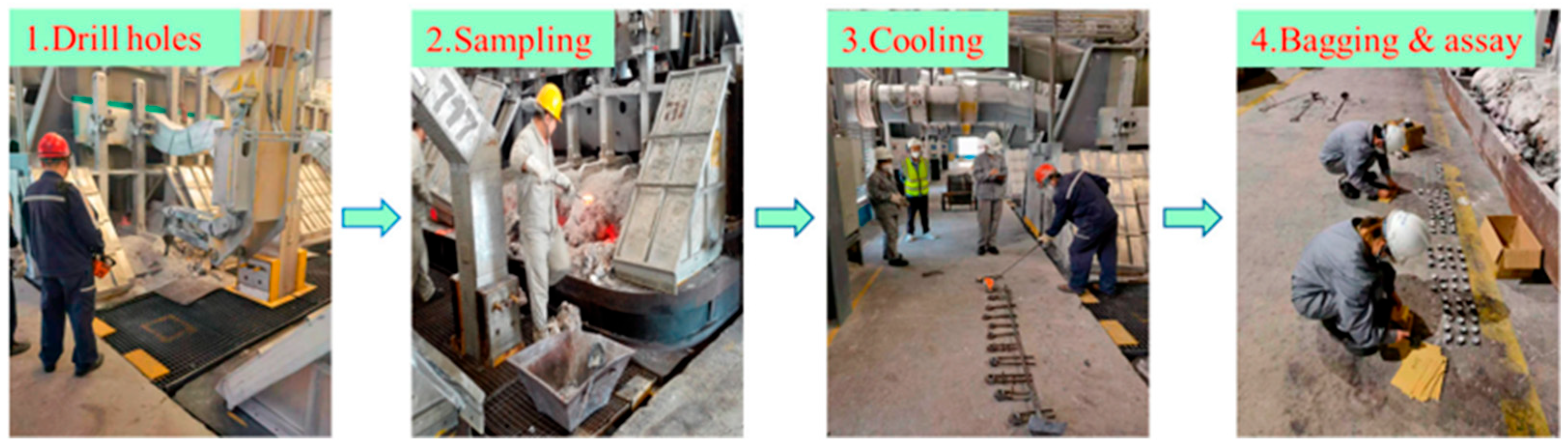
Due to extreme operating conditions such as high temperature, strong magnetic fields, and multi-field coupling, as well as the complexity of the process environment, there is a lack of online detection equipment for alumina concentration that meets the actual production requirements in industrial sites. As shown in Figure 6, current alumina concentration measurements still rely on traditional manual sampling and laboratory analysis methods. The operational process includes on-site drilling and sampling, sample cooling, packaging, and sending the samples to the laboratory for analysis. This offline detection method has obvious lag, making it impossible to achieve real-time monitoring and control of alumina concentration during the production process.
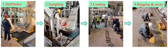
Figure 6.
Data sample collection process.
A total of 600 samples of alumina concentration data were collected on-site. Focusing on alumina concentration (Y) as the key controlled variable, corresponding process parameters—including anode voltage at both poles (X1 and X2) and anode conductor current (X3)—were retrieved from the production monitoring system as auxiliary variables. This resulted in a structured industrial dataset containing 600 data groups, as shown in Table 3.
Table 3.
Structured industrial dataset.
The experiment divided the 600 valid samples into a training set (500 samples) and a test set (100 samples) at a ratio of 5:1. To eliminate the interference caused by differences in units on model training, a min–max normalization method was applied to standardize the multi-source heterogeneous data. This preprocessing step significantly improved the model’s convergence speed and generalization ability by ensuring consistency in the distribution of input and output feature spaces, thereby providing a reliable data foundation for subsequent intelligent algorithm modeling. The normalization formula is as follows:
where is the normalized value, is the original value, is the maximum value of the selected samples, and is the minimum value of the selected samples.
3.2. Model Evaluation Metrics
The model’s goodness of fit and accuracy determine its performance, which can be evaluated using the coefficient of determination (), root mean square error (), mean absolute error (), and accuracy. The specific calculation formulas are as follows:
where denotes the variance. A larger value (closer to 1) indicates smaller errors between the predicted and actual values in the sample, reflecting better explanatory power of the independent variables on the dependent variable in regression analysis—hence, higher prediction accuracy of the model. represents the actual value, and denotes the predicted value. Usually, smaller RMSE and MAE values mean the model’s predictions are more accurate.
3.3. Design of the Soft-Sensing Model
This study creates a soft-sensing model to predict alumina concentration by combining the weighted average algorithm (WAA) with a long short-term memory (LSTM) network. The design steps are as follows:
First, the collected data are normalized to fit within a set range, which helps the model enhance training efficiency and convergence speed. After preprocessing the data, the candidate solutions are set up, and the fitness of each one is calculated. This step is important to check how good the solutions are and, for the soft-sensing model, it means checking how accurate the predictions are.
Next, the best position of each individual and the overall best position in the current round are found. These guide the next search steps. Then, the weighted average position—an important part of the WAA—is calculated to balance searching widely and focusing closely. The judgment criterion k1 is updated using the weighted average position.
The positions of candidate solutions are then checked to make sure they meet the boundary conditions. After confirming the boundary conditions, the fitness values of the current candidate solutions are recalculated to assess whether the updated positions are improved. Based on the new fitness values, the personal best and global best positions are updated. This iterative process continues until the preset maximum number of iterations is reached.
Upon reaching the maximum number of iterations, the optimized parameters are output and used to construct the final soft-sensing model. These optimal parameters are then employed to train the LSTM model. Once training is complete, the test sample set is input into the trained LSTM model to verify the model’s performance. The overall workflow of the proposed model is illustrated in Figure 7.
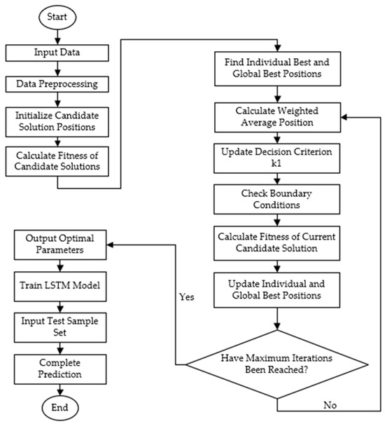
Figure 7.
Flowchart of the WAA-LSTM-based soft-sensing model design.
4. Comparative Analysis of Model Results
4.1. Results of Hyperparameter Optimization for Different Models
The optimal number of neurons, number of layers, learning rate, batch size, and number of training epochs for each neural network model—obtained through hyperparameter optimization using the WAA—are shown in Table 4.
Table 4.
Parameter settings of different prediction models.
4.2. Comparison of Simulation Results for Different Models
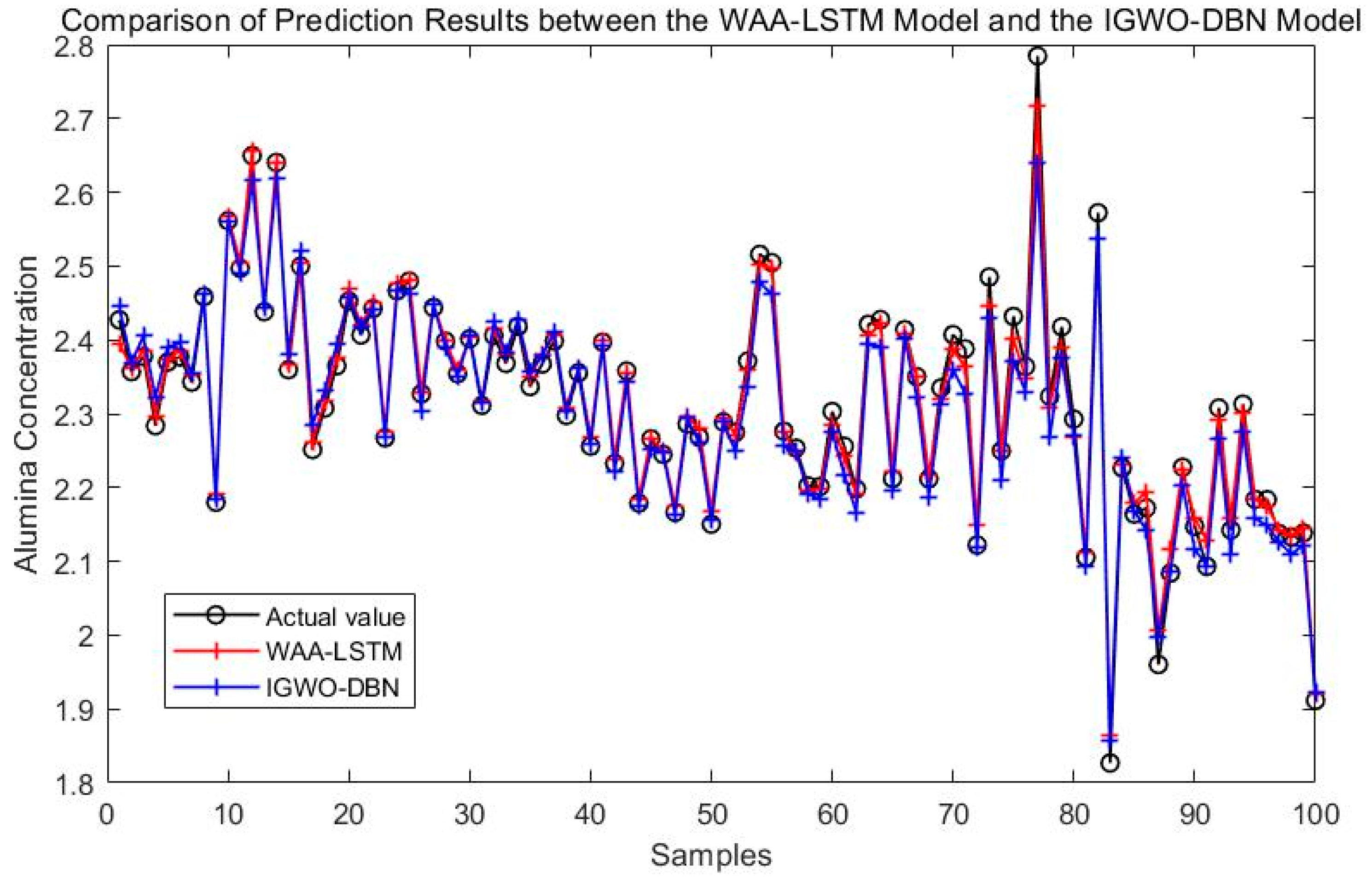
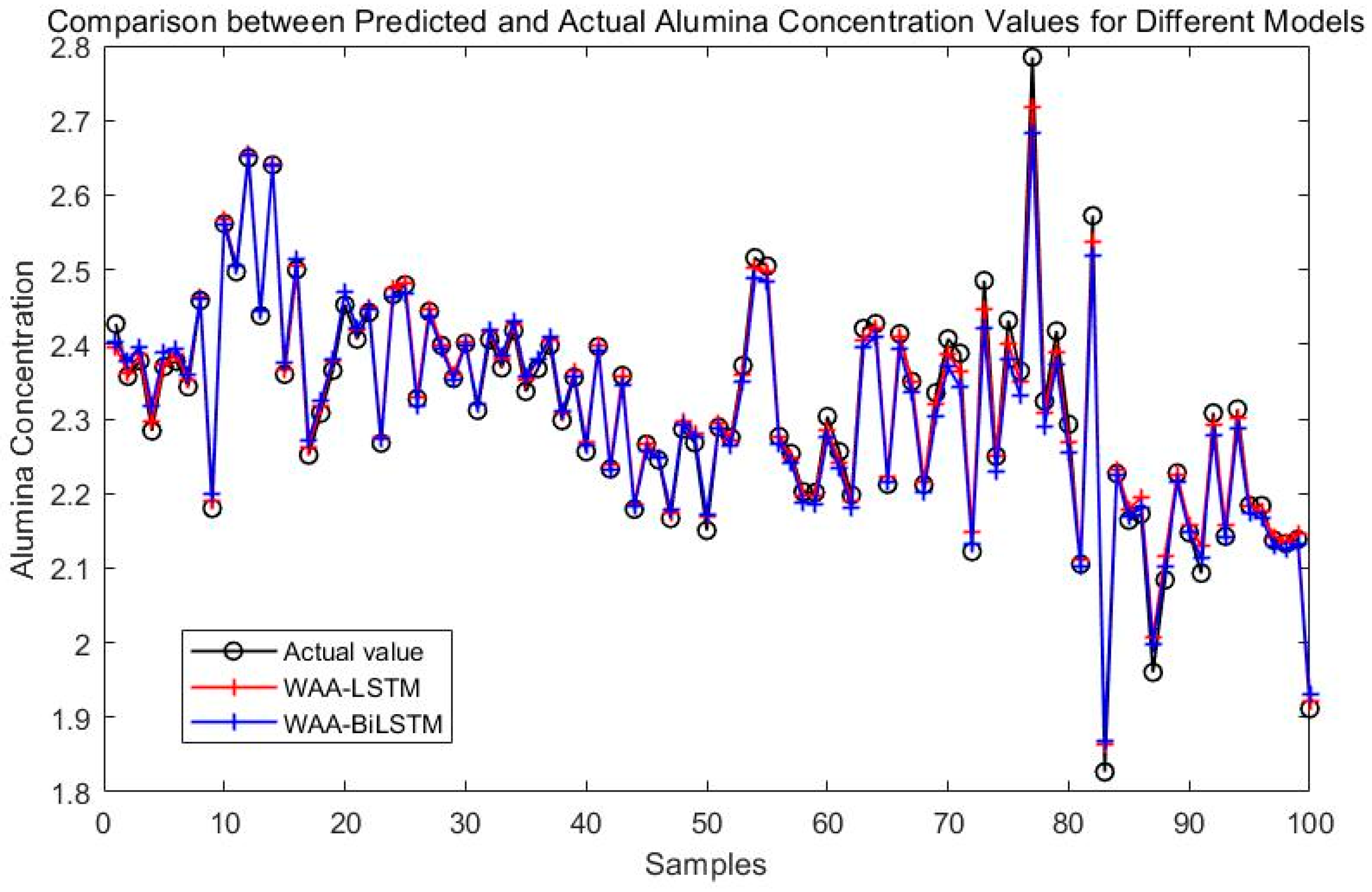
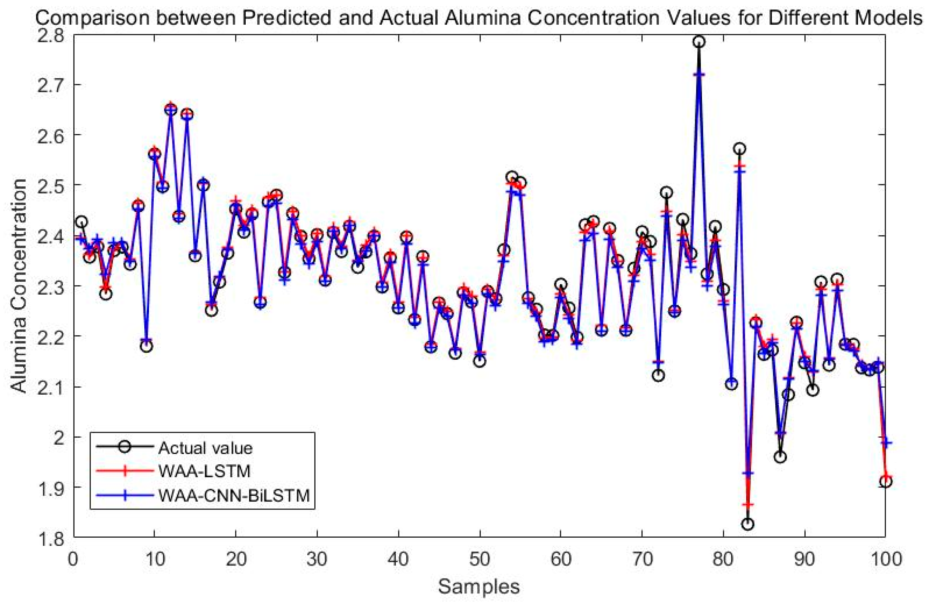
To assess the effectiveness of the proposed WAA-LSTM network, a comparative analysis is conducted against the IGWO-enhanced DBN model. As illustrated in Figure 8, simulation results demonstrate the performance of the proposed method. For comparison, several state-of-the-art models, including BiLSTM, CNN-LSTM, CNN-BiLSTM, CNN-LSTM-Attention, and CNN-BiLSTM-Attention, are also evaluated. After hyperparameter optimization, the respective simulation results are presented in Figure 9.
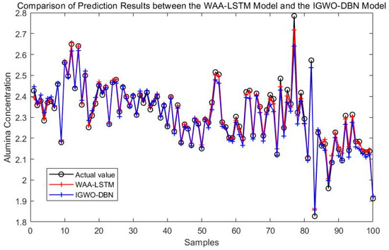
Figure 8.
Comparison of prediction results between the WAA-LSTM model and the IGWO-DBN model.
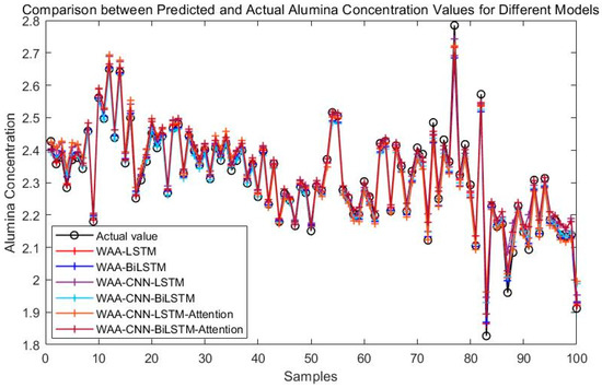
Figure 9.
Comparison between predicted and actual alumina concentration values for different models.
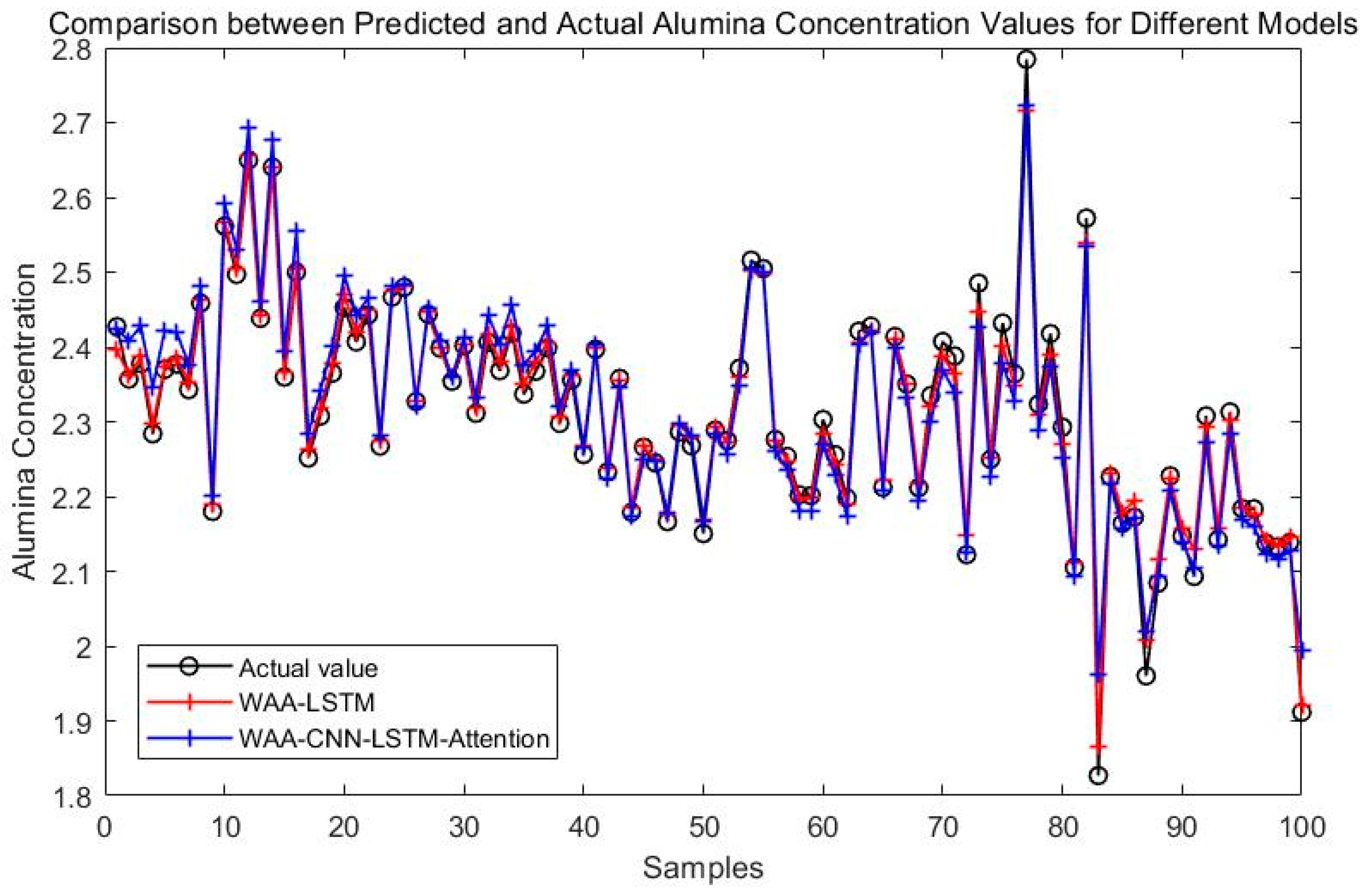
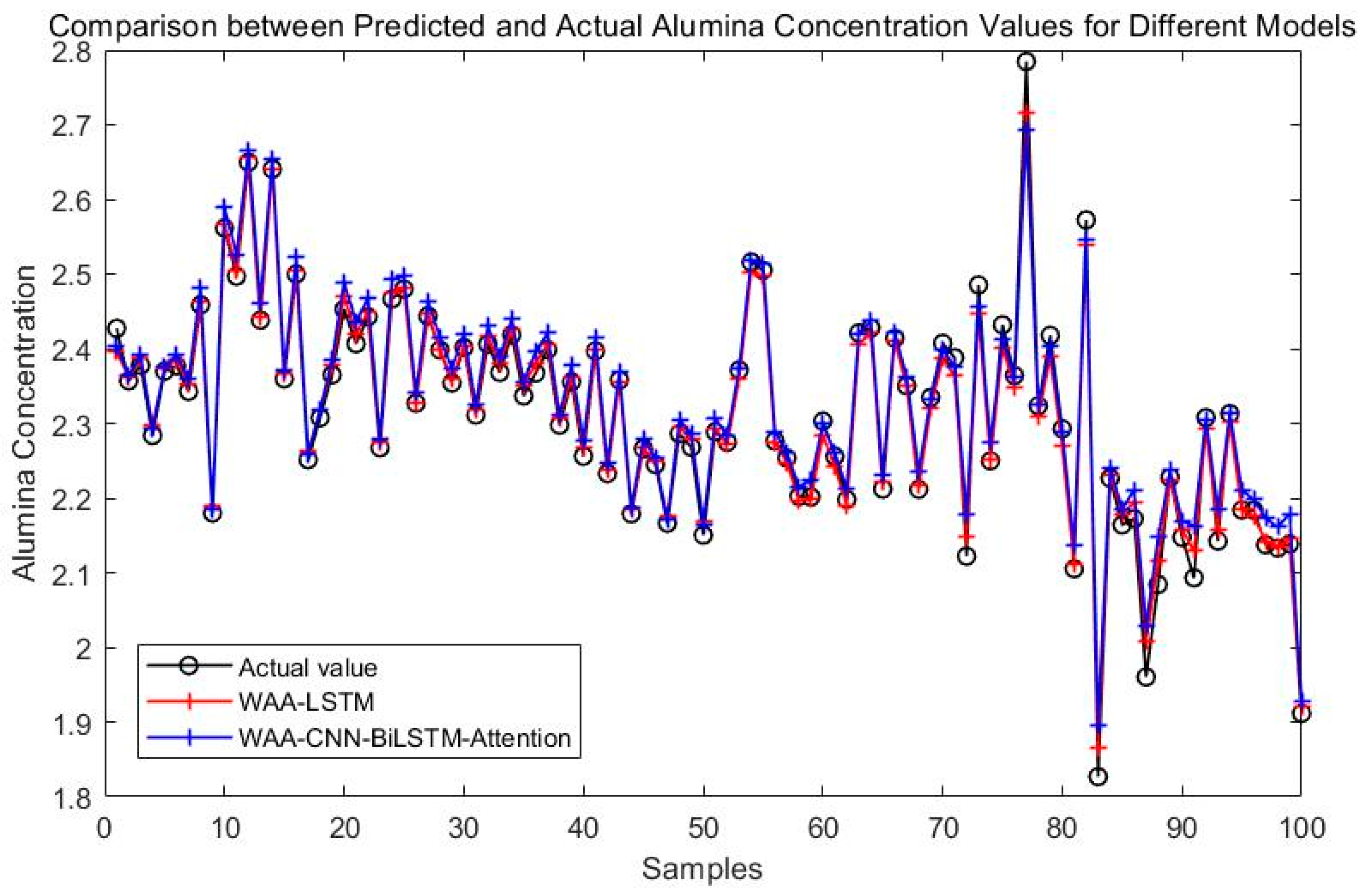
Figure 8 compares the prediction performance of the WAA-LSTM and IGWO-DBN models. The WAA-LSTM model demonstrates superior accuracy and stability. As shown in Figure 9, Figure 10, Figure 11, Figure 12, Figure 13 and Figure 14, the predicted values of the WAA-LSTM model (red line) closely align with the actual values (black circles) across most samples, indicating high prediction accuracy. The WAA-LSTM model exhibits smaller prediction fluctuations than WAA-BiLSTM, WAA-CNN-LSTM, WAA-CNN-BiLSTM, WAA-CNN-LSTM-Attention, and WAA-CNN-BiLSTM-Attention, indicating superior stability. Furthermore, the WAA-LSTM model effectively captures the overall variation trend of alumina concentration, which is largely consistent with the trend of the actual values.

Figure 10.
Comparison between WAA-LSTM and WAA-BiLSTM.
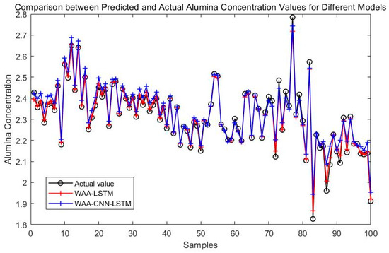
Figure 11.
Comparison between WAA-LSTM and WAA-CNN-LSTM.
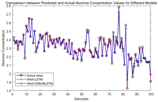
Figure 12.
Comparison between WAA-LSTM and WAA-CNN-BiLSTM.

Figure 13.
Comparison between WAA-LSTM and WAA-CNN-LSTM-Attention.
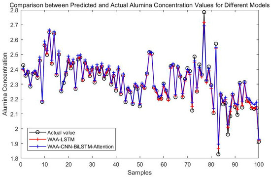
Figure 14.
Comparison between WAA-LSTM and WAA-CNN-BiLSTM-Attention.
Table 5 demonstrates that the WAA-LSTM model outperforms the IGWO-DBN model on all key metrics. The WAA-LSTM achieves an MAE of 0.0117, RMSE of 0.0161, and R2 of 0.9883, whereas IGWO-DBN yields 0.0209, 0.0285, and 0.9685, respectively. Additionally, under error limits of 5%, 2%, and 1%, the WAA-LSTM attains accuracies of 1.0000, 0.9700, and 0.8700, respectively, significantly surpassing IGWO-DBN’s 0.9900, 0.9500, and 0.6200. These results demonstrate the superior accuracy and stability of the WAA-LSTM model in predicting alumina concentration.
Table 5.
Comparison of prediction results for different models.
Even though the WAA-CNN-LSTM and WAA-CNN-LSTM-Attention models use CNN structures and attention to improve feature extraction, they do not perform better than the WAA-LSTM model. Models like WAA-BiLSTM, WAA-CNN-BiLSTM, and WAA-CNN-BiLSTM-Attention improve with bidirectional LSTM structures, helping them better understand time-based relationships and perform well on most metrics. However, their accuracy under the strictest 1% error threshold is slightly lower than that of the WAA-LSTM model, suggesting that unidirectional LSTM may hold an advantage in scenarios requiring extremely high precision.
5. Optimization Algorithm Comparison and Analysis
5.1. Parameter Optimization Results of Different Algorithms
The optimal numbers of neurons, layers, learning rates, batch sizes, and iteration counts for the LSTM neural network model, optimized, respectively, by the WAA, Grey Wolf Optimizer (GWO), Harris Hawks Optimizer (HHO), Optuna, Tornado optimizer with Coriolis force (TOC), and Whale Migrating Algorithm (WMA), are presented in Table 6.
Table 6.
Parameter optimization results of LSTM models using different optimization algorithms.
5.2. Comparison of Simulation Results for Different Optimization Algorithms
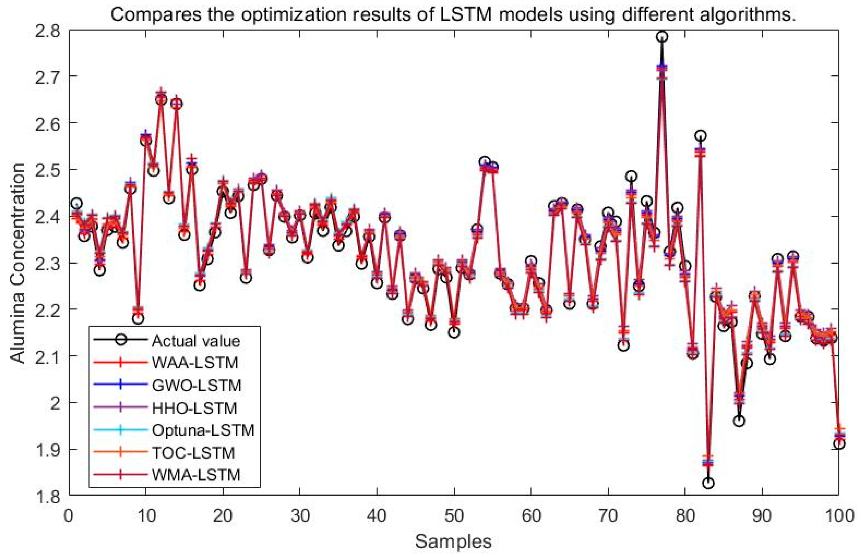
The simulation results of the LSTM neural network model optimized by the WAA, GWO, HHO, Optuna, TOC, and WMA are shown in Figure 15.

Figure 15.
Compares the optimization results of LSTM models using different algorithms.
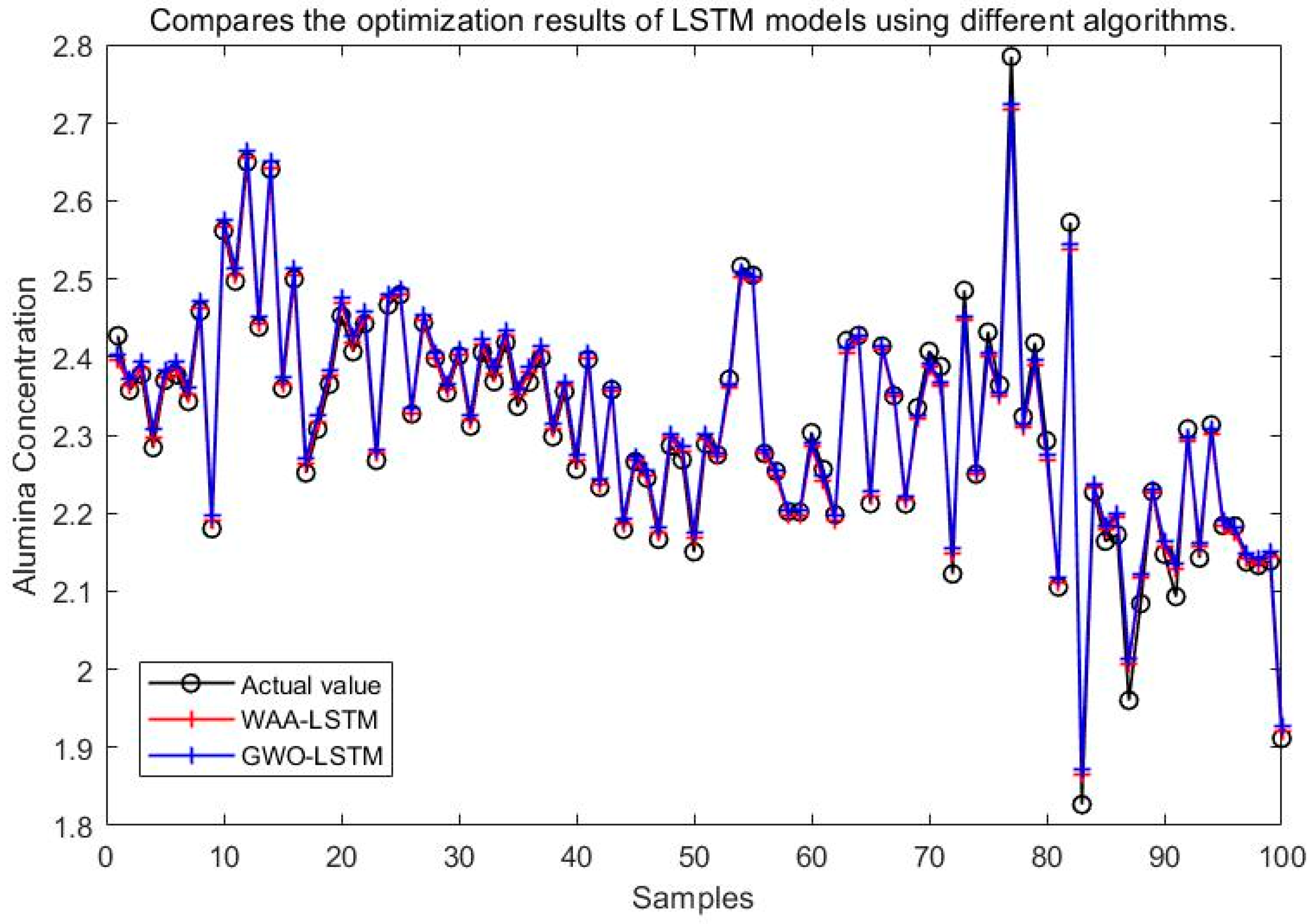
It can be seen from Figure 15, Figure 16, Figure 17, Figure 18, Figure 19 and Figure 20 that the LSTM model optimized by the WAA outperforms other models in overall performance, showing a higher degree of fit between its predicted curve and the actual values in the alumina concentration prediction task. The WAA-LSTM model exhibits rapid loss reduction in the early training stages, indicating strong convergence. As training progresses, the loss steadily decreases, reaching the lowest validation loss. The GWO-LSTM model performs comparably, trailing slightly behind. The HHO-LSTM, Optuna-LSTM, TOC-LSTM, and WMA-LSTM models maintain good performance during training but are marginally inferior to WAA-LSTM and GWO-LSTM. Overall, as shown in Figure 21, the WAA-LSTM model achieves stable training performance and the lowest final loss.
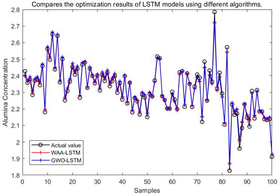
Figure 16.
Comparison between WAA-LSTM and GWO-LSTM.
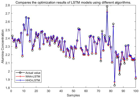
Figure 17.
Comparison between WAA-LSTM and HHO-LSTM.
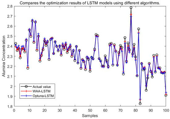
Figure 18.
Comparison between WAA-LSTM and Optuna-LSTM.
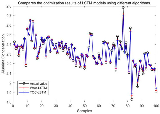
Figure 19.
Comparison between WAA-LSTM and TOC-LSTM.
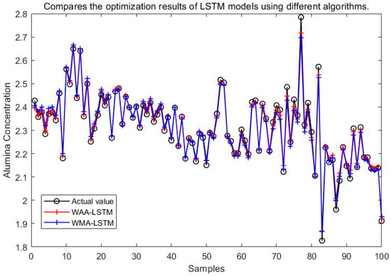
Figure 20.
Comparison between WAA-LSTM and WMA-LSTM.
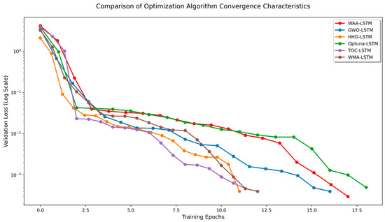
Figure 21.
Comparison of convergence characteristics of optimization algorithms.
Table 7 presents the evaluation metrics for six models: WAA-LSTM, GWO-LSTM, HHO-LSTM, Optuna-LSTM, TOC-LSTM, and WMA-LSTM. Among these, WAA-LSTM and GWO-LSTM demonstrate similar accuracy levels. However, for the MAE and RMSE metrics, the WAA-LSTM model clearly achieves lower values than the other models, confirming its superior effectiveness and prediction accuracy.
Table 7.
Comparison of prediction results optimized by different algorithms.
6. Statistical Analysis and Hypothesis Testing
6.1. Principles of Statistical Hypothesis Testing
This section focuses on the twelve hybrid prediction frameworks constructed in Section 4 and Section 5, evaluating them uniformly on 100 independent test samples to identify systematic differences in accuracy and robustness among the various algorithms. A non-parametric statistical approach—the Friedman test followed by Nemenyi post-hoc analysis—is employed to systematically evaluate model performance and further verify the relative advantage of the proposed WAA-LSTM model in terms of predictive accuracy.
The Friedman test, proposed by statistician Milton Friedman, is a non-parametric statistical method suitable for scenarios involving multiple algorithms and repeated measurements [34]. Let the null hypothesis be that there is no significant difference in the average ranks of all models regarding overall performance. For each test sample, the absolute percentage errors (APE) of the 12 models are ranked from smallest to largest, denoted as . Subsequently, the average rank of model over the 100 samples is calculated. The formulas for calculating the absolute percentage error (APE) and average rank are as follows:
Friedman test statistic:
It follows a distribution with degrees of freedom, where and . If or the corresponding -value is less than 0.05, the null hypothesis , which states that all models have equal average ranks, is rejected.
When the Friedman test rejects the null hypothesis, the Nemenyi test is introduced to identify the sources of difference. It is used as a non-parametric post-hoc multiple comparison method following the Friedman test to determine whether there are significant differences between groups [35]. The critical difference () is calculated as follows:
where is the critical value from the Studentized range distribution. If the difference in average ranks between two models, , exceeds the , it is concluded that there is a statistically significant difference between models and l (equivalently, ).
6.2. Results and Visualization
In this experiment, the Friedman test yielded a test statistic of , with a corresponding -value of approximately , which is far below the threshold of 0.05. This indicates that there are significant overall performance differences among the 12 hybrid models in terms of the APE metric. Table 8 summarizes the APE metrics for each model. The WAA-LSTM model exhibits the lowest median, mean, and standard deviation—0.37%, 0.51%, and 0.48%, respectively—initially indicating superior performance, characterized by both high accuracy and low variability.
Table 8.
Comparison of APE values across different models.
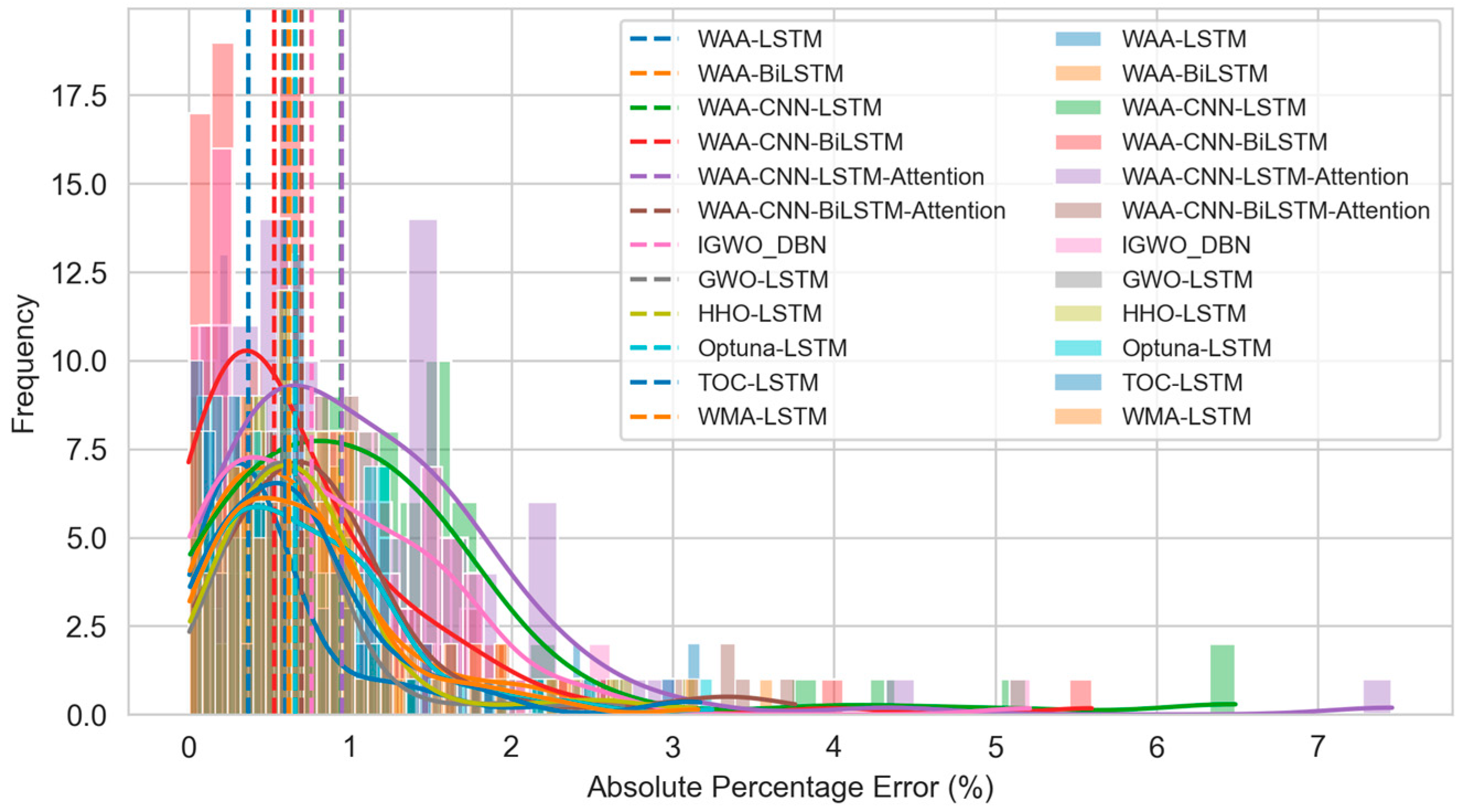
The histogram and kernel density curve in Figure 22 further depict the distribution of prediction errors. The WAA-LSTM model exhibits the flattest box and the fewest outliers, further confirming the model’s effectiveness and accuracy. To further validate the significant advantage of the WAA-LSTM model, Figure 23 presents a heatmap of -values based on the Nemenyi test. In the heatmap, darker colors indicate more significant differences between models. It is evident from the figure that the row and column corresponding to WAA-LSTM contain the highest proportion of dark-colored cells, indicating that the performance differences between WAA-LSTM and most other models are statistically significant.
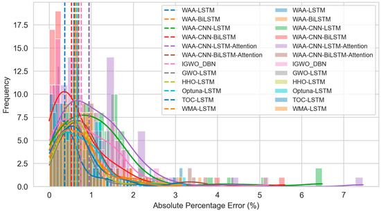
Figure 22.
Boxplots of APE distributions for each model.
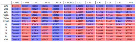
Figure 23.
Heatmap of p-values from the Nemenyi post-hoc test.
Remark 2.
For ease of presentation in the p-values heatmap, model names have been abbreviated. Table 9 provides the list of abbreviations.
Table 9.
Model full names and their abbreviations.
7. Conclusions
The present study successfully proposes an alumina concentration prediction model based on the long short-term memory (LSTM) neural network optimized via the weighted average algorithm (WAA). The model employs automated hyperparameter optimization using the WAA to determine the optimal LSTM architecture—specifically, the number of hidden units and layers—as well as training parameters such as learning rate, batch size, and number of epochs. By balancing training efficiency and model performance, the model achieves an optimal configuration, whose generalization capability is subsequently evaluated on a test dataset. This method significantly reduces the complexity of manual parameter tuning while enhancing model performance.
Experimental results demonstrate that the WAA-LSTM model outperforms the IGWO-DBN model across all key evaluation metrics. The WAA-LSTM model exhibits high accuracy and stability in predicting alumina concentration. To further validate its superiority, comparisons were made with hybrid models including WAA-BiLSTM, WAA-CNN-LSTM, WAA-CNN-BiLSTM, WAA-CNN-LSTM-Attention, and WAA-CNN-BiLSTM-Attention. Although the WAA-CNN-LSTM and WAA-CNN-LSTM-Attention models introduce convolutional structures and attention mechanisms to enhance feature extraction, their performance does not surpass that of the WAA-LSTM model. Similarly, models incorporating bidirectional LSTM structures (WAA-BiLSTM, WAA-CNN-BiLSTM, and WAA-CNN-BiLSTM-Attention) demonstrate improved comprehension of data and achieve competitive results in most evaluation metrics. However, their accuracy under the strictest 1% error threshold is slightly inferior to that of the WAA-LSTM model, indicating that unidirectional LSTM may offer advantages under low-tolerance error conditions. The WAA-LSTM model is compared with GWO-LSTM, HHO-LSTM, Optuna-LSTM, TOC-LSTM, and WMA-LSTM. In terms of convergence, WAA-LSTM demonstrates stable performance throughout the training process, achieving the lowest final loss, which indicates better generalization and robustness. Finally, its effectiveness and accuracy are further confirmed through the Friedman test and subsequent Nemenyi post-hoc analysis.
In practical aluminum electrolysis operations, the WAA-LSTM model can be seamlessly integrated into existing data acquisition and control systems to receive real-time inputs such as cell voltage and anode beam current, enabling online prediction of alumina concentration. The prediction outcomes facilitate optimized alumina feeding strategies and dynamic adjustment of electrolysis process parameters, thereby effectively preventing issues such as abnormal oxygen evolution, reduced electrolysis efficiency, and even damage to the electrolytic cell caused by concentration fluctuations. By optimizing electrolysis process parameters and regulating production efficiency, dynamic monitoring of alumina concentration stability is achieved, providing more reliable data support for intelligent decision-making systems in the production process, thereby enhancing industrial automation and control capabilities.
Nonetheless, the study has certain limitations; a complete theoretical framework for alumina concentration prediction is still lacking, especially with regard to dynamic modeling and mechanism integration under complex operating conditions. Future research should focus on two key areas: (1) reducing prediction bias in soft-sensing models through multi-source data fusion and improved feature engineering, and (2) integrating deep learning approaches with mechanistic models to further enhance the accuracy and real-time performance of concentration prediction.
Author Contributions
Conceptualization, X.L. and Y.W.; methodology, X.X.; validation, J.L.; formal analysis, Y.W.; resources, X.L.; writing—original draft preparation, X.X.; writing—review and editing, X.L. and J.L.; visualization, X.X.; supervision, X.L.; project administration, X.L.; funding acquisition, X.L. All authors have read and agreed to the published version of the manuscript.
Funding
This work is jointly supported by Natural Science Foundation Project of JiangXi Province, Grant Number 20242BAB25091; Natural Science Foundation Project of Guizhou Province, Grant Number ZK[2023] General004; and Science and Technology Project of Jiangxi Provincial Department of Education, Grant Number GJ2202404.
Data Availability Statement
The datasets presented in this article are not readily available. Requests to access the datasets should be directed to 21021@jdzu.edu.cn.
Conflicts of Interest
The authors declare no conflicts of interest.
References
- Liu, X.; Yang, Y.; Wang, Z.; Tao, W.; Li, T.; Zhao, Z. CFD modeling of alumina diffusion and distribution in aluminum smelting cells. JOM 2019, 71, 764–771. [Google Scholar] [CrossRef]
- Yao, Y.; Cheung, C.; Bao, J.; Skyllas-Kazacos, M.; Welch, B.; Akhmetov, S. Estimation of spatial alumina concentration in an aluminum reduction cell using a multilevel state observer. AIChE J. 2017, 63, 2806–2818. [Google Scholar] [CrossRef]
- Moxnes, B.; Solheim, A.; Liane, M.; Svinsas, E.; Halkjelsvik, A. Improved cell operation by redistribution of the alumina feeding. In Proceedings of the TMS Light Metals, San Antonio, TX, USA, 15–19 February 2009; pp. 461–466. Available online: https://www.researchgate.net/publication/283249275_Improved_cell_operation_by_redistribution_of_the_alumina_feeding (accessed on 22 July 2025).
- Hou, W.; Li, H.; Mao, L.; Cheng, B.; Feng, Y. Effects of electrolysis process parameters on alumina dissolution and their optimization. Trans. Nonferrous Met. Soc. China 2020, 30, 3390–3403. [Google Scholar] [CrossRef]
- Yan, Q.; Liang, J.; Liu, B.; Cui, J.; Li, Q.; Huang, R. Predictive Control of Alumina Concentration Based on Recursive Subspace. J. Beijing Univ. Technol. 2023, 49, 467–474. [Google Scholar] [CrossRef]
- Geng, D.; Pan, X.; Yu, H.; Tu, G.; Yu, D. Real-Time Automatic Detection of Sodium Aluminate Solution Concentration Based on PSO-BP Neural Network. JOM 2025, 77, 3263–3274. [Google Scholar] [CrossRef]
- Zhu, J.; Xu, Y.; Cao, B.; Cehng, J. Research on Alumina Concentration Prediction in Aluminum Electrolysis Cells Based on PSO-LSTM for the Aluminum Industry. Light Met. 2023, 7, 21–27. [Google Scholar] [CrossRef]
- Du, S.; Huang, Y.; Lu, S.; Shi, J.; Zhang, H. Dynamic Simulation of Alumina Concentration Based on Distributed Sensing. Nonferrous Met. (Extr. Metall.) 2023, 11, 26–32. [Google Scholar] [CrossRef]
- Cao, Z. Research on Alumina Concentration Prediction in Aluminum Electrolysis Cells Optimized by Improved Quantum Genetic Algorithm. Master’s Degree, Central South University, Changsha, China, 2023. [Google Scholar] [CrossRef]
- Li, Y. A Novel Soft Sensor Model for Alumina Concentration Based on Collaborative Training SDBN. In Proceedings of the 2024 IEEE 13th Data Driven Control and Learning Systems Conference (DDCLS), Kaifeng, China, 17–19 May 2024; pp. 1751–1755. [Google Scholar] [CrossRef]
- Ma, L.; Wong, C.; Bao, J.; Skyllas-Kazacos, M.; Welch, B.; Li, W.; Shi, J.; Ahli, N.; Aljasmi, A.; Mahmoud, M. H∞ Filter-based Alumina Concentration Estimation for an Aluminium Smelting Process. IFAC-Pap. 2024, 58, 36–41. [Google Scholar] [CrossRef]
- Ma, L.; Wong, C.; Bao, J.; Skyllas-Kazacos, M.; Shi, J.; Ahli, N.; Aljasmi, A.; Mahmoud, M. Estimation of the Spatial Alumina Concentration of an Aluminium Smelting Cell Using a Huber Function-Based Kalman Filter. In Light Metals 2024; Wagstaff, S., Ed.; TMS 2024—The Minerals, Metals and Materials Series; Springer: Cham, Switzerland, 2024; pp. 464–473. [Google Scholar] [CrossRef]
- Huang, R.; Li, Z.; Cao, B. A Soft Sensor Approach Based on an Echo State Network Optimized by Improved Genetic Algorithm. Sensors 2020, 20, 5000. [Google Scholar] [CrossRef] [PubMed]
- Li, X.; Liu, B.; Qian, W.; Rao, G.; Chen, L.; Cui, J. Design of Soft-Sensing Model for Alumina Concentration Based on Improved Deep Belief Network. Processes 2022, 10, 2537. [Google Scholar] [CrossRef]
- Li, J.; Chen, Z.; Zhong, X.; Li, X.; Xia, X.; Liu, B. Design of Soft-Sensing Model for Alumina Concentration Based on Improved Grey Wolf Optimization Algorithm and Deep Belief Network. Processes 2025, 13, 606. [Google Scholar] [CrossRef]
- Choudhary, S.; Kumar, G. Enhancing link prediction in dynamic social networks through hybrid GCN-LSTM models. Knowl. Inf. Syst. 2025. [Google Scholar] [CrossRef]
- Wang, C.; Li, Q.; Cui, J.; Wang, Z.; Ma, L. CNN-LSTM-based Prediction of the Anode Effect in Aluminum Electrolytic Cell. In Proceedings of the 2022 41st Chinese Control Conference (CCC), Hefei, China, 25–27 July 2022; pp. 4112–4117. [Google Scholar] [CrossRef]
- Pala, M. Graph-Aware AURALSTM: An Attentive Unified Representation Architecture with BiLSTM for Enhanced Molecular Property Prediction. Mol. Divers. 2025. [Google Scholar] [CrossRef] [PubMed]
- Andika, N.; Wongso, P.; Rohmat, F.; Wulandari, S.; Fadhil, A.; Rosi, R.; Burnama, N. Machine learning-based hydrograph modeling with LSTM: A case study in the Jatigede Reservoir Catchment, Indonesia. Results Earth Sci. 2025, 3, 100090. [Google Scholar] [CrossRef]
- Reimers, N.; Gurevych, I. Optimal Hyperparameters for Deep LSTM-Networks for Sequence Labeling Tasks. arXiv 2017. [Google Scholar] [CrossRef]
- Wang, Z.; Wang, Q.; Wu, T. A novel hybrid model for water quality prediction based on VMD and IGOA optimized for LSTM. Front. Environ. Sci. Eng. 2023, 17, 88. [Google Scholar] [CrossRef]
- Li, G.; Wang, Y.; Xu, C.; Wang, J.; Fang, X.; Xiong, C. BO-STA-LSTM: Building energy prediction based on a Bayesian optimized spatial-temporal attention enhanced LSTM method. Dev. Built Environ. 2024, 18, 100465. [Google Scholar] [CrossRef]
- Li, X.; Lin, J.; Liu, C.; Liu, A.; Shi, Z.; Wang, Z.; Jiang, S.; Wang, G.; Liu, F. Research on Aluminum Electrolysis from 1970 to 2023: A Bibliometric Analysis. JOM 2024, 76, 3265–3274. [Google Scholar] [CrossRef]
- Snoek, J.; Larochelle, H.; Adams, R. Practical bayesian optimization of machine learning algorithms. Adv. Neural Inf. Process. Syst. 2012, 25, 2951–2959. Available online: https://proceedings.neurips.cc/paper/2012/hash/05311655a15b75fab86956663e1819cd-Abstract.html (accessed on 22 July 2025).
- Hochreiter, S.; Schmidhuber, J. Long short-term memory. Neural Comput. 1997, 9, 1735–1780. [Google Scholar] [CrossRef] [PubMed]
- Sherstinsky, A. Fundamentals of recurrent neural network (RNN) and long short-term memory (LSTM) network. Phys. D Nonlinear Phenom. 2020, 404, 132306. [Google Scholar] [CrossRef]
- Xu, G.; Meng, Y.; Qiu, X.; Yu, Z.; Wu, X. Sentiment analysis of comment texts based on BiLSTM. IEEE Access 2019, 7, 51522–51532. [Google Scholar] [CrossRef]
- Luo, J.; Zhang, X. Convolutional neural network based on attention mechanism and bi-lstm for bearing remaining life prediction. Appl. Intell. 2022, 52, 1076–1091. [Google Scholar] [CrossRef]
- Brauwers, G.; Frasincar, F. A General Survey on Attention Mechanisms in Deep Learning. IEEE Trans. Knowl. Data Eng. 2021, 35, 3279–3298. [Google Scholar] [CrossRef]
- Liu, L.; Tian, X.; Ma, Y.; Lu, W.; Luo, Y. Online soft measurement method for chemical oxygen demand based on CNN-BiLSTM-Attention algorithm. PLoS ONE 2024, 19, e0305216. [Google Scholar] [CrossRef] [PubMed]
- Cheng, J.; Waele, W. Weighted average algorithm: A novel meta-heuristic optimization algorithm based on the weighted average position concept. Knowl.-Based Syst. 2024, 305, 112564. [Google Scholar] [CrossRef]
- Chai, Q.; Zhang, S.; Tian, Q.; Yang, C.; Guo, L. Daily Runoff Prediction Based on FA-LSTM Model. Water 2024, 16, 2216. [Google Scholar] [CrossRef]
- Zhu, J. Research on Predicting Alumina Concentration in Electrolytic Cells for Aluminum Industry; Guizhou University: Guiyang, China, 2024. [Google Scholar] [CrossRef]
- Friedman, M. The use of ranks to avoid the assumption of normality implicit in the analysis of variance. J. Am. Stat. Assoc. 1937, 32, 675–701. [Google Scholar] [CrossRef]
- Nemenyi, P. Distribution-Free Multiple Comparisons; Princeton University: Princeton, NJ, USA, 1963; Available online: https://www.proquest.com/openview/c1f3e8829e8351e9c2a1c5e51778c6cf/1?pq-origsite=gscholar&cbl=18750&diss=y (accessed on 22 July 2025).


Disclaimer/Publisher’s Note: The statements, opinions and data contained in all publications are solely those of the individual author(s) and contributor(s) and not of MDPI and/or the editor(s). MDPI and/or the editor(s) disclaim responsibility for any injury to people or property resulting from any ideas, methods, instructions or products referred to in the content. |
© 2025 by the authors. Licensee MDPI, Basel, Switzerland. This article is an open access article distributed under the terms and conditions of the Creative Commons Attribution (CC BY) license (https://creativecommons.org/licenses/by/4.0/).