Predicting Monthly Wind Speeds Using XGBoost: A Case Study for Renewable Energy Optimization

Abstract

This study presents a wind speed prediction model using monthly average wind speed data, employing the Extreme Gradient Boosting (XGBoost) algorithm to enhance forecasting accuracy for wind farm operations. Accurate wind speed forecasting is crucial for optimizing energy production, ensuring grid stability, and improving operational planning. Existing studies on enhancing wind speed prediction using ML algorithms have some drawbacks based on accuracy, efficient prediction, and stuck-in-local-optima parameters. The dataset comprises monthly average wind speed measurements, and extensive preprocessing is conducted to prepare the data for machine learning. Various hyperparameter tuning techniques, including Randomized Search, Grid Search, and Bayesian Optimization, are applied to improve prediction accuracy. The performance of the model is evaluated utilizing key metrics, including Mean Absolute Error (MAE), Root Mean Squared Error (RMSE), Mean Absolute Percentage Error (MAPE), Continuous Ranked Probability Score (CRPS), and Maximum Error. The results indicate that hyperparameter tuning significantly improves model accuracy. Specifically, Grid Search demonstrates superior performance for short-term (one-month) forecasting, while Randomized Search is more effective for long-term (six-month) forecasting. The findings emphasize the critical importance of hyperparameter tuning strategies in the development of reliable wind speed forecasting models, which have significant implications for the efficient management of wind energy resources.

1. Introduction

Wind energy has emerged as one of the most promising renewable sources due to its environmental benefits and growing potential for generating clean, sustainable electricity [1,2]. As the world shifts toward renewable energy to reduce reliance on fossil fuels and mitigate climate change, wind energy plays a pivotal role in this transition, aligning with the United Nations Sustainable Development Goals (SDGs), particularly Goal 7: Affordable and Clean Energy, and Goal 13: Climate Action [3,4,5,6]. Efficient energy harvesting from wind turbines and seamless integration of wind-generated power into the electricity grid requires accurate wind speed prediction [7]. Wind speed forecasting aids in optimizing power generation, improving grid stability, and reducing operational uncertainty, which often hinders the effective use of renewable energy [8,9]. Despite the importance of wind speed prediction, wind’s inherently stochastic and volatile nature makes accurate forecasting endeavors challenging.

The challenge lies in the fluctuating characteristics of wind, which are influenced by numerous environmental factors and conditions. Wind speed can vary significantly due to geographical features, atmospheric conditions, and weather patterns, resulting in substantial difficulty in creating predictive models that generalize well under different conditions [10,11,12]. Conventional statistical approaches have often fallen short in capturing the complex, non-linear relationships between these factors and wind speed, leading to inaccuracies in forecasting.

Table 1. Literature review of advanced wind speed prediction models and their methodological contributions.

Ref.	Model/Methodology	Dataset Location	Key Limitation
[13]	CNN-LSTM Hybrid Neural Network	New Zealand (Gore Ews, Lake Karapiro Cws, Baring Head)	Reduced performance for long intervals, high computational cost
[14]	EWT-ARIMA-LSSVM-GPR-DE-GWO	Xuanwei, Yunnan, China	Model complexity, high computational expense
[15]	GRU with Attention Mechanism	Hangzhou–Haining; Norway Railways	Complexity and computational cost for high-dimensional data
[16]	EMD-RNN-ARIMA	Inner Mongolia, China	Computational complexity for large datasets
[17]	CNN-BLSTM-Attention (Grid Search Optimized)	Flatirons Campus, Colorado, USA	High computational complexity, limited experimental validation
[18]	PSO-Bi-LSTM with VMD	Southeast China (Offshore Wind Farm)	Model complexity, high computational cost
[19]	SSA-ConvLSTM Hybrid	NREL (Various Seasonal Data)	Computational complexity, challenging for real-time
[20]	TVFEMD-PACF-IChOA-BiGRU	Prince William Sound, Alaska, USA	High resource requirements, complex optimization stages
[21]	ORedRVFL (AOA and VMD optimized)	Louisiana, USA (Atchafalaya River)	Hyperparameter optimization, resource-intensive
[22]	PSO-VMD-SE-ICEEMDAN with Att-S2S	Paso Robles, Oasis Wind Farm, California, USA	Multi-layer decomposition complexity, high resource needs
[23]	DWT-BiLSTM-BiGRU Hybrid	Galicia, Spain; Kerman, Iran	Preprocessing and decomposition complexity
[24]	WGformer (WGT, Informer, Kernel MSE)	Barrow, Alaska; Summit, Greenland; South Pole (NOAA)	High-dimensional kernel, preprocessing complexity
[25]	Hybrid Prediction Framework	Sotavento Wind Farm, Galicia, Spain	Multi-stage complexity, computational cost
[26]	MST-GNN (Wind-Transformer)	Denmark, Netherlands (5 and 7 Cities)	Spatial–temporal prediction complexity
[27]	EMD-KM-SXL (SVR, XGBoost, Lasso)	Matang, Jiangsu, China (SCADA Data)	Multi-stage decomposition, integration complexity
[28]	BFS-BiLSTM Hybrid	European Meteorological Data (6 years)	Multi-phase learning, high complexity

highlights various advanced models for wind speed prediction, integrating neural networks, hybrid deep learning frameworks, and machine learning algorithms. Key methodologies include CNN-LSTM hybrids, GRU with attention, EWT-ARIMA-LSSVM-GPR-DE-GWO, and BiLSTM approaches optimized with techniques like PSO, VMD, and empirical decompositions. Datasets span global locations such as China, the USA, New Zealand, and Europe, reflecting diverse environmental conditions. Despite significant advancements in prediction accuracy and feature extraction, a recurring limitation across studies is the high computational complexity and resource demand, particularly during data preprocessing, hyperparameter optimization, and multi-stage decomposition. This often restricts the real-time application and scalability of these models.

In the field of wind energy forecasting, the prediction of monthly average wind speeds holds substantial value for long-term planning, including resource allocation and grid stability. While daily and hourly forecasts are typically used for operational purposes, monthly predictions are crucial for broader energy policy development and for understanding the potential for wind energy generation over extended periods. Monthly averages allow energy planners to assess the overall feasibility of wind energy projects, evaluate seasonal wind variations, and optimize the placement of wind farms to maximize efficiency. Despite the non-linear nature of wind power generation, predicting monthly averages is integral to making informed decisions about wind energy investment and grid integration [29,30,31,32].

Studies have demonstrated CRPS as a robust metric for evaluating probabilistic wind forecasts [33]. Its advantage over traditional metrics lies in simultaneously assessing calibration and sharpness of predictive distributions [34], particularly valuable for operational wind farm management [35].

The forecasting of wind speed is a critical component in optimizing wind energy generation and grid integration. Several methods, including machine learning techniques such as XGBoost, have been applied to predict wind speed. However, the performance of these models significantly depends on the choice of hyperparameters, which can influence model accuracy and predictive power. Hyperparameter optimization is essential to enhance model performance, and various techniques have been proposed, including Grid Search, Random Search, and more recent methods like Bayesian Optimization. While the existing literature has primarily focused on the forecasting techniques themselves, fewer studies have systematically evaluated the impact of hyperparameter tuning for improving prediction accuracy in wind speed forecasting models. Few articles from existing literature reviews does not provide significant results, as mentioned in

Table 2. Recently Used Models with evaluation metrics focus on quantitative performance comparisons.

Ref. No	Year	Model	Evaluation Metrics
[36]	2022	SVM	MAE = 1.04, MSE = 1.85, RMSE = 1.36
		ANN	MAE = 0.98, MSE = 1.71, RMSE = 1.31
[37]	2023	XGBoost	MSE = 1.662, RMSE = 1.289, MAE = 0.996, MAPE = 48.46
		SARIMAX	MSE = 2.212, RMSE = 1.487, MAE = 2.949, MAPE = 99.88
		ARIMA	MSE = 1.266, RMSE = 1.604, MAE = 1.985, MAPE = 76.02
[38]	2022	XGBoost (Optimized)	MAPE = 12.96, RMSE = 20.85
		XGBoost	MAPE = 17.95, RMSE = 21.89
		ANN	MAPE = 17.95, RMSE = 21.89
		SARIMA	MAPE = 56.47, RMSE = 66.29
[39]	2022	SVM	MAE = 9.02, RMSE = 11.74
		LSTM	MAE = 9.02, RMSE = 11.74
		BH-XGBoost	MAE = 6.52, RMSE = 9.29
		XGBoost	MAE = 9.02, RMSE = 11.76

. The evaluation metrics for each study are taken directly from the respective publications. Since not all authors reported the same performance indicators (like MAE, MSE, RMSE, MAPE), we have preserved the metrics as originally presented, leading to variations in completeness across entries. This paper, therefore, focuses on the comparison of hyperparameter optimization approaches applied to XGBoost, a widely used machine learning model, for forecasting wind speed. By comparing different hyperparameter tuning methods, this study aims to provide insights into their effectiveness in improving model performance.

Accurate wind speed prediction is crucial for optimizing wind energy systems and ensuring their reliable integration into power grids. However, the inherent variability and complexity of wind patterns, influenced by geographical, atmospheric, and weather-related factors, pose significant challenges. Traditional statistical methods often fail to capture the non-linear and dynamic nature of wind speed, necessitating advanced machine learning approaches for improved forecasting.

This study aims to enhance wind speed prediction by employing a robust machine learning framework. Utilizing preprocessed average monthly wind speed data, the research explores advanced optimization techniques, including Randomized Search, Grid Search, and Bayesian Optimization, to refine the predictive model’s accuracy and generalizability. The goal is to develop more effective prediction methods that address the complexities of wind energy forecasting. By systematically evaluating the impact of different optimization strategies, this research contributes to the advancement of wind speed prediction techniques, supporting the global transition toward sustainable energy systems. The findings aim to provide a replicable framework for future studies, ultimately aiding in the efficient utilization of wind resources and promoting global sustainability efforts. This work focuses on methodological improvements, emphasizing the refinement of prediction techniques and their practical implications in renewable energy applications.

The remaining parts of this paper are organized as follows. Section 2 describes the dataset. The methodology in Section 3 describes the algorithm, model implementation, hyperparameter tuning techniques, training of the model, and the evaluation metrics. The results and discussion in Section 4 provide a comparative analysis of each model’s performance. Section 5 consists of the conclusion that offers recommendations for future research on the exploration of advanced optimization techniques and hybrid tuning methodologies to enhance the robustness and generalizability of models.

2. Dataset Description

This Section provides a comprehensive overview of the dataset, including details about the data collected, its structure, and its purpose. The dataset used in this study contains monthly average wind speed data from January 2018 to July 2024. Each data point represents the average wind speed for a specific month, with features including ’month’ and ’year’. The dataset was meticulously cleaned to address inconsistencies and rectify any missing values. Subsequently, normalization techniques were implemented to ensure that all features were standardized and maintained on a uniform scale. The preprocessed data were then used as input for training the XGBoost model. Figure 1a illustrates the average wind speed for each month throughout the specified period after preprocessing, measured in meters per second (m/s). Typically, wind speeds exhibit an upward trend from January, attaining peak values in May, June, and July, with average measurements ranging from 7 to 8 m/s. Wind speed declines from September, reaching its lowest levels during October and November. The accompanying chart highlights that summer months are characterized by the highest wind speeds, whereas autumn and winter months exhibit significantly lower wind speeds. Figure 1b presents the annual average wind speed from 2018 to 2024 after preprocessing, measured in meters per second (m/s). The average wind speed fluctuates slightly over the years, with the highest recorded average occurring in 2018, reaching approximately 6.5 m/s. The year 2024 has recorded the lowest average wind speed, which is slightly below 6 m/s, based on data available up to July. Overall, wind speeds have demonstrated a relatively stable pattern over the years, exhibiting only minor fluctuations in average measurements.

The dataset used in this study was collected from Jhimpir, Sindh, Pakistan, a significant wind energy corridor. The data were recorded using a Supervisory Control and Data Acquisition (SCADA) system, ensuring precise and high-quality measurements. The dataset contains monthly average wind speed data from January 2018 to July 2024, with each data point representing the average wind speed for a specific month. Figure 2 presents a time-series visualization of SCADA-measured wind speed (in meters per second) across multiple years and months. The upper panel shows monthly wind speed variations, with peaks typically occurring around mid-year (June–August), suggesting seasonal patterns. The lower panel aggregates data by year, revealing potential interannual variability or trends in wind speeds. This analysis helps identify optimal periods for energy generation and maintenance planning.

During preprocessing, the dataset was carefully examined for inconsistencies and missing values. No missing values were found, and the data were already in a standardized format suitable for direct input into the model. Therefore, while normalization techniques are often used to scale numerical features, they were not required in this case, as the wind speed values were naturally consistent across the dataset. The preprocessed data were then used for training the XGBoost model.

3. Methodology

The methodology comprises multiple phases, including data collection, preprocessing, feature extraction and selection, model development, and evaluation. Each phase is essential for ensuring a comprehensive and effective approach to the overall process. Initially, historical wind speed data are collected and subjected to preprocessing procedures to address missing values and remove outliers. Subsequently, relevant features are extracted and selected to optimize predictive performance. The XGBoost algorithm is utilized to model the wind speed data effectively. Hyperparameter tuning is conducted using three different techniques to optimize the model performance: Grid Search, Randomized Search, and Bayesian Optimization. The evaluation of the model is conducted using several metrics, including Mean Absolute Error (MAE), Mean Absolute Percentage Error (MAPE), Maximum Error, and Root Mean Squared Error (RMSE). The methodology flow is depicted in Figure 3. Figure 3 presents the proposed end-to-end pipeline for monthly wind speed forecasting. The workflow commences with SCADA-based historical wind speed data and proceeds through a preprocessing phase. This phase is visually represented by the preprocessed dataset. Following this, the framework extracts relevant temporal features before performing training and prediction using the XGBoost algorithm. Additionally, the figure includes the mathematical expressions for five evaluation metrics (MAE, MSE, RMSE, R², and MAPE) that quantify the model’s performance.

3.1. Algorithm Overview

The architecture of XGBoost is comprised of several stages, including feature processing, boosting iterations, and evaluation. It commences with an input layer that contains a feature matrix, in which each row represents an individual sample, and each column corresponds to a specific feature. In addition, there exists a label vector (y) that denotes the target variable. The boosting process starts with an initial prediction, usually set to zero. In the first iteration, the gradient of the loss function is calculated concerning the current predictions, and a decision tree is fitted to approximate the negative gradients (errors). The model predictions are then updated based on the output of this tree. Subsequent iterations involve sequentially adding trees to correct residual errors from the previous iterations, with predictions being updated after each new tree is added. Each weak learner, or tree, contributes to adjusting the model’s predictions by fitting to residual errors and learning to minimize these errors. Regularization and shrinkage play a critical role in the architecture, where each tree’s complexity is controlled to prevent overfitting by penalizing deeper or more complex trees. Additionally, a learning rate (n) is used as a shrinkage factor to scale each tree’s contribution, ensuring robustness and reducing the risk of overfitting. After completing k iterations, the final output consists of the aggregated predictions made by all the trees, as shown in Figure 4. The mathematical formulation of the XGBoost algorithm is based on an ensemble of decision trees, where it incrementally builds trees to minimize a loss function. The objective function of XGBoost consists of two parts: a loss function and a regularization term, as shown in Equation (1) [40].

$$\mathcal{L}\left(\theta \right)=\sum _{i=1}^{n}l\left(y_i,{\widehat{y}}_i\right)+\sum _{k=1}^K\mathrm{\Omega }{(f}_k)$$

(1)

where $l\left(y_i,{\widehat{y}}_i\right)$ is a loss function that measures the difference between the prediction ${(\widehat{y}}_i)$ and the true label ($y_i$). Usually, the squared error is used for regression or logistic loss for classification. $\mathrm{\Omega }{(f}_k)$ is a regularization term that penalizes the complexity of the trees to prevent overfitting. $K$ is the number of trees in the ensemble. $f_k$ is a decision tree (the $k^{th}$ tree in the model). The regularization term is generally of the form as in Equation (2).

$$\mathrm{\Omega }(f)=\gamma T+{\displaystyle \frac{1}{2}}\lambda \sum _{j=1}^T{\omega }_j^2$$

(2)

where T is the number of leaves in the tree. ω is the score for leaf j, and $\gamma$ and $\lambda$ are regularization parameters that control the model complexity.

The XGBoost model is built in an additive manner, which means that trees are added sequentially, as in Equation (3)

$${\widehat{y}}_i^{\left(t\right)}={\widehat{y}}_i^{(t-1)}+f_t(x_i)$$

(3)

where ${\widehat{y}}_i^{\left(t\right)}$ is the prediction of instance i after t iterations. $f_t$ is the newly added decision tree. To minimize the objective function at each step t, a new tree $f_t$ is added to minimize the loss, ${\mathcal{L}}^{\left(t\right)}$ represents the loss function at the t-th iteration as shown in Equation (4)

$${\mathcal{L}}^{\left(t\right)}=\sum _{i=1}^{n}l\left(y_i,{\widehat{y}}_i^{\left(t-1\right)}+f_t\left(x_i\right)\right)+\mathrm{\Omega }{(f}_t)$$

(4)

A second-order approximation (Taylor expansion) of the loss function is used, as in Equation (5).

$${\mathcal{L}}^{\left(t\right)}\approx {\sum }_{i=1}^n\left[g_i{f}_t\left(x_i\right)+{\displaystyle \frac{1}{2}}{h}_i{f}_t^2\left(x_i\right)\right]+\mathrm{\Omega }{(f}_t)$$

(5)

The first-order gradient is as in Equation (6), and the second-order gradient (Hessian) is in Equation (7)

$$g_i={\displaystyle \frac{\partial l(y_i,{\widehat{y}}_i^{\left(t-1\right)})}{\partial {\widehat{y}}_i^{\left(t-1\right)}}}$$

(6)

$$h_i={\displaystyle \frac{{\partial }^{2}l(y_i,{\widehat{y}}_i^{\left(t-1\right)})}{\partial {\widehat{y}}_i^{{\left(t-1\right)}^2}}}$$

(7)

The tree’s structure is determined by selecting splits that maximize the gain. The gain from a split is computed as in Equation (8)

$$Gain={\displaystyle \frac{1}{2}}[{\displaystyle \frac{{{(G}_L+G_R)}^2}{H_L+H_R}}-{\displaystyle \frac{G_L^2}{H_L+\lambda }}-{\displaystyle \frac{G_R^2}{H_R+\lambda }}]$$

(8)

where $G_L \mathrm{a}\mathrm{n}\mathrm{d} G_R$ are gradient sums for the left and right child nodes, $H_L \mathrm{a}\mathrm{n}\mathrm{d} H_R$ are Hessian sums for the left and right child nodes, and $\gamma \mathrm{a}\mathrm{n}\mathrm{d} \lambda$ are regularization parameters. XGBoost uses the computed gain to determine whether a particular split should be performed in the decision tree. After all trees are built, the final prediction is the sum of the outputs from all the trees, as in Equation (9)

$${\widehat{y}}_i=\sum _{k=1}^K{f}_x\left(x_i\right)$$

(9)

The model was developed using Python 3.12.4 within the Visual Studio Code environment, employing libraries such as scikit-learn, pandas, and XGBoost. The initial model was constructed with default parameters, followed by the application of hyperparameter tuning techniques to enhance its performance. The selected features for the model included ‘month’ and ‘year’, while the target variable represented the monthly average wind speed.

Figure 4 also depicts an infographic that illustrates the proposed framework for monthly wind speed forecasting utilizing the XGBoost algorithm, specifically within the realm of renewable energy optimization. This framework leverages historical wind data and employs optimization techniques to fine-tune the XGBoost model, resulting in accurate forecasts that enhance renewable energy applications. It also tackles key challenges, such as seasonal variability and forecasting error, through focused model tuning.

3.2. Hyperparameter Tuning Techniques

To improve the performance of the XGBoost model, three distinct methods of hyperparameter tuning were employed: Grid Search, Randomized Search, and Bayesian Optimization. These methods were chosen to explore the hyperparameter space efficiently while balancing computational cost and model accuracy.

(i)

Grid Search: Grid Search is a comprehensive approach that systematically explores a predefined set of hyperparameter values. This method evaluates all possible combinations within the specified ranges to identify the best-performing configuration [41]. Despite its effectiveness in fine-tuned optimization, Grid Search can be computationally expensive, particularly when dealing with a large number of hyperparameters. In this study, Grid Search was applied to systematically evaluate combinations of hyperparameters such as n_estimators, max_depth, learning_rate, subsample, and colsample_bytree, ensuring optimal model performance. The range is selected as ‘n_estimators’: [50, 100, 150, 200], ‘max_depth’: [3, 5, 7, 9], ‘learning_rate’: [0.01, 0.05, 0.1, 0.3], ‘subsample’: [0.6, 0.7, 0.8, 0.9], and ‘colsample_bytree’: [0.6, 0.7, 0.8, 0.9].

(ii)

Random Search: Randomized Search offers a more efficient alternative to Grid Search by randomly sampling hyperparameter values instead of exhaustively evaluating all possible combinations. This approach allows a broader exploration of the parameter space while significantly reducing computational time [41,42]. Randomized Search is particularly beneficial when the search space is large, as it increases the likelihood of identifying an optimal configuration without the need for an exhaustive search. In this study, Randomized Search was used to efficiently explore different hyperparameter settings, aiming to strike a balance between computational efficiency and model accuracy. The parameter grid for randomized search were selected as ‘n_estimators’: randint(50, 200), ‘max_depth’: randint(3, 10), ‘learning_rate’: uniform(0.01, 0.3), ‘subsample’: uniform(0.6, 0.9), and ‘colsample_bytree’: uniform(0.6, 0.9).

(iii)

Bayesian Optimization: Bayesian Optimization is a probabilistic approach that leverages past evaluation results to build a model of the objective function and determine the next set of hyperparameters to test. Unlike Grid and Randomized Search, Bayesian Optimization focuses on finding an optimal set of hyperparameters while minimizing the number of evaluations [43]. It employs a surrogate model (typically a Gaussian process) to predict the most promising hyperparameter configurations, ensuring an efficient search strategy. In this study, Bayesian Optimization was used as the initial tuning method to effectively balance model complexity and generalization, improving performance while reducing computational costs. The search space for Bayesian is ‘n_estimators’: Integer(50, 200), ‘max_depth’: Integer(3, 10), ‘learning_rate’: Real(0.01, 0.3), ‘subsample’: Real(0.6, 0.9), and ‘colsample_bytree’: Real(0.6, 0.9).

In this study, the XGBoost algorithm was initially implemented with default hyperparameter values. To improve model performance, three different hyperparameter tuning techniques were applied: Bayesian Optimization, Grid Search, and Randomized Search.

Table 3. Best hyperparameter values found by different Tuning Methods.

Parameters	XGBoost (Default Parameters)	Bayesian-XGBoost	Grid Search-XGBoost	Randomized Search-XGBoost
n-estimators	100	200	50	178
Nax-depth	6	3	3	3
Learning-rate	0.3	0.0223	0.1	0.019
subsample	1	0.7079	0.6	0.815
Colsample-bytree	1	0.6501	0.6	0.9699

presents the optimized hyperparameters obtained through each approach. First, Bayesian Optimization was used to tune XGBoost, resulting in optimized hyperparameter values that balance model complexity and generalization. Next, Grid Search was applied, systematically evaluating a predefined set of hyperparameter combinations to identify the best-performing configuration. Finally, Randomized Search was employed, randomly sampling hyperparameter values from a given range to efficiently explore the search space. The best-selected hyperparameters from each tuning method are reported in Table 3. The impact of these optimized hyperparameters on model performance is analyzed in the Results Section, where the predictive accuracy of each configuration is compared.

3.3. Training the Model

The model employed the average monthly wind speed as the dependent variable, with the month and year functioning as independent variables. Historical data on monthly average wind speeds were utilized to forecast the wind speed for the subsequent month. Furthermore, the model facilitated extended forecasts by predicting wind speeds for the following six months, thereby providing valuable insights into potential future wind patterns.

The dataset was split temporally (80% training, 20% testing) without shuffling to preserve time-series order. The model utilizes data from all previous months’ wind speeds as input to predict the current month’s average, comparing the results against mean-based and linear regression baselines. The dataset encompassing the period from January 2018 to July 2024 is systematically partitioned into training and testing sets. The training set comprised data from January 2018 through December 2022, totaling 60 months, while the testing set covered the subsequent period from January 2023 to July 2024, amounting to 15 months. Input variables were extracted from Supervisory Control and Data Acquisition (SCADA) measurements, which were then aggregated into monthly means through the application of arithmetic averaging. The temporal split is implemented as follows:

• One-Month-Ahead Predictions
  Training: The model is trained once on the full 60-month training set, covering the period from January 2018 to December 2022.
  Testing: It is evaluated on a 15-month test set from January 2023 to July 2024 without any retraining, ensuring a true out-of-sample assessment.
• Six-Month-Ahead Predictions
  Walk-forward validation is employed to address longer-term dependencies: Initial training is conducted from 1 to 60 months (January 2018 to December 2022), followed by testing on months from 61 to 66 (January to June 2023). The model is then retrained on months 1 through 61 (January 2018 to January 2023) and tested on months 62 to 67 (February to July 2023). This process is repeated until the final test window, which spanned months 70 to 75 (October 2023 to July 2024).

To quantify the uncertainty in our wind speed predictions, we estimated confidence intervals using quantile regression with XGBoost. The difference between predictions defines the confidence band, providing an interval within which the actual wind speed values are expected to fall. In this study, a 90% confidence interval was used, ensuring that 90% of future wind speeds should lie within the estimated range.

3.4. Evaluation Metrics

The model’s performance was evaluated using five distinct metrics. The Mean Absolute Error (MAE) was utilized to quantify the average absolute deviation between the predicted and actual wind speeds, providing an overall measure of error magnitude. The Mean Absolute Percentage Error (MAPE) assessed the prediction accuracy as a percentage of the actual values, indicating the relative error of the model’s predictions. Root Mean Squared Error (RMSE) was employed to evaluate the model’s sensitivity to larger deviations, as it applies a greater penalty to larger errors, offering a more comprehensive measure of prediction inaccuracy. The Maximum Error metric was used to determine the largest deviation between predicted and actual values, thereby identifying the most severe inaccuracies in the model’s predictions. The relevant equations are presented in Figure 3.

To strengthen our forecasting evaluation, we incorporate the Continuous Ranked Probability Score (CRPS) alongside traditional point forecast metrics. The CRPS measures the difference between the predicted cumulative distribution function $F\left(y\right)$ and the observed value $y_{oes}$, calculated as in Equation (10):

$$CRPS=\underset{-\infty }{\overset{\infty }{\int }}{\left[F\left(y\right)-(y\ge y_{oes})\right]}^{2}dy$$

(10)

We employ CRPS as it properly accounts for both forecast reliability and resolution, unlike point-estimate metrics like MAE. This aligns with best practices in renewable energy forecasting [44,45]. For our XGBoost implementation, we generate probabilistic forecasts through quantile regression, estimating the 10th, 50th, and 90th percentiles using the ‘reg:quantileerror’ objective. The predictive distribution is constructed via linear interpolation between these quantiles. All CRPS calculations are performed using the properscoring Python library, ensuring consistency with established practices. This probabilistic framework provides a more comprehensive assessment of forecast quality by simultaneously evaluating both the accuracy (sharpness) and uncertainty calibration (reliability) of our predictions.

4. Results and Discussion

XGBoost (Extreme Gradient Boosting) is an ensemble learning algorithm that builds multiple decision trees sequentially to optimize performance. It is known for its speed and accuracy, particularly in regression and classification tasks. XGBoost uses gradient boosting to combine weak learners into a stronger model while incorporating L1 and L2 regularization to prevent overfitting [46,47]. The XGBoost model exhibited notable effectiveness in forecasting monthly average wind speeds. We computed the Mean Absolute Error (MAE), Root Mean Square Error (RMSE), Mean Absolute Percentage Error (MAPE), and Maximum Error metrics for both the initial model and the model subsequent to hyperparameter tuning. The results following the tuning process illustrated substantial enhancements, particularly through Bayesian optimization, which yielded the lowest values for both MAE and RMSE.

Figure 5 presents a detailed analysis of historical wind speeds, forecasted values, and corresponding confidence intervals, offering a comprehensive examination of the variability in wind speed and the associated model predictions. The historical data, represented by the blue line from 2018 to 2024, demonstrate marked fluctuations, featuring peaks near 9 m/s and troughs below 4 m/s, which reflect the inherent dynamics of the atmospheric environment. Notably, the highlighted blue point indicates the forecasted wind speed for the forthcoming month of August, projected to be approximately 8 m/s, signifying a substantial increase relative to recent observations. This forecast implies a potential escalation in wind activity, suggesting a significant rise in wind speeds during the upcoming period. The visualization adeptly encapsulates the temporal fluctuations in wind speed while providing insights into the anticipated future trend as predicted by the employed model. The forecasted wind speeds, delineated by the orange line and derived from an XGBoost predictive model, indicate an expected increase to around 8 m/s for August 2024, followed by a gradual decline to 5 m/s in subsequent months. This projected decrease contrasts sharply with prior peaks, indicating a potential reduction in wind speed during the forecasted timeframe. The visual representation effectively illustrates historical wind speed variations while elucidating the expected trend over the subsequent six months as predicted by the model. This short-term increase, coupled with a longer-term decline, suggests a shift in wind patterns that may significantly impact energy planning initiatives. The shaded confidence interval, encompassing a 90% range, quantitatively assesses prediction uncertainty, with broader intervals indicative of greater variability during specific periods. This interval effectively represents the range between the 10th and 90th percentile predictions, capturing the expected variability in wind speed and providing a probabilistic measure of uncertainty essential for reliable energy planning and integration into grid operations.

The confidence interval further delineates that the predictions exhibit a degree of variability, with the shaded region expanding or contracting in accordance with the anticipated accuracy of the forecast. This visual representation enriches our understanding of historical fluctuations, projected future trends, and the uncertainty range, underscoring the variability intrinsic to wind speed predictions. By amalgamating these elements, Figure 5 proficiently communicates both the observed trends and the reliability of future projections, thereby highlighting the critical importance of probabilistic forecasting in the management of renewable energy resources.

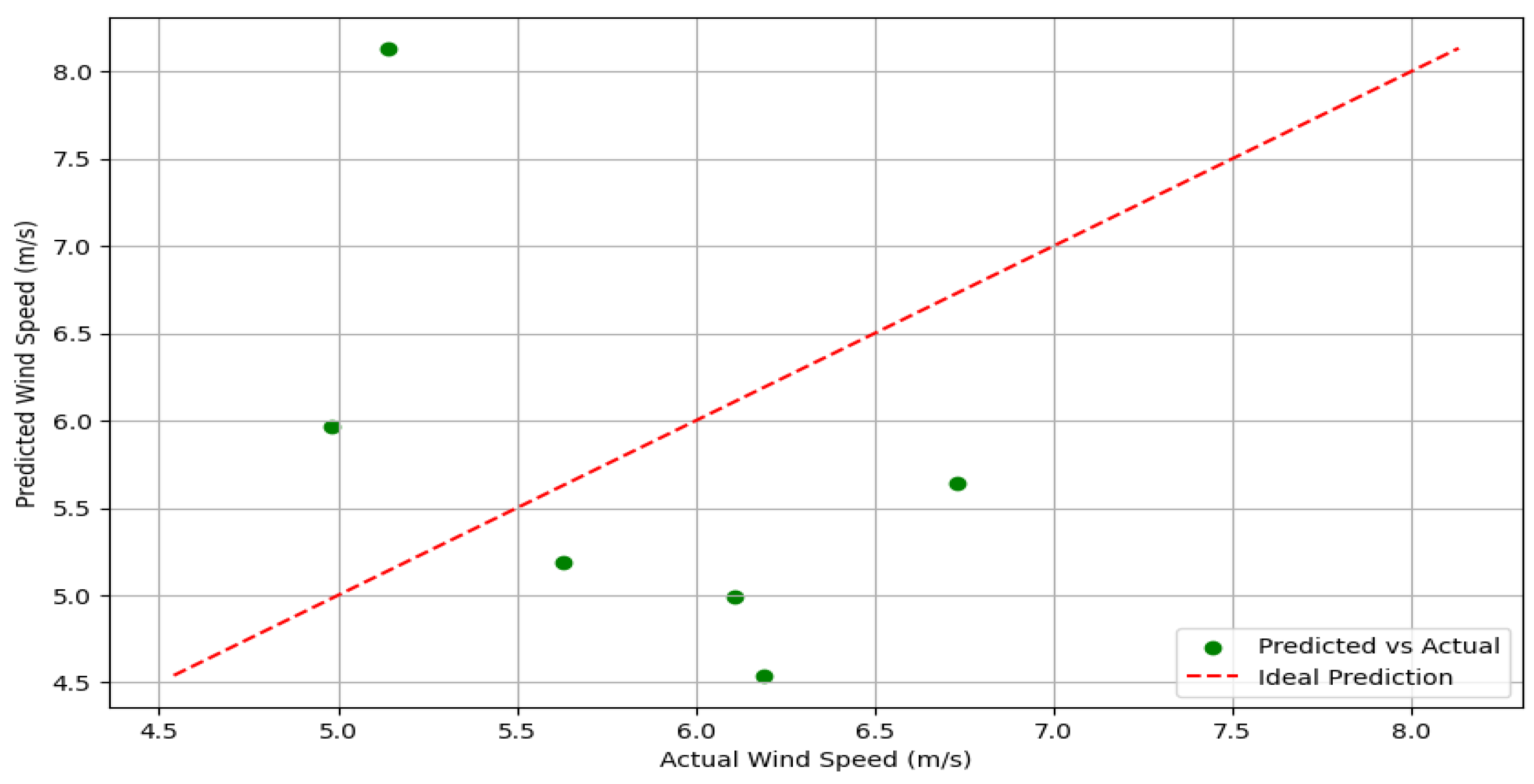
Figure 6 presents the relationship between actual and predicted wind speeds for an XGBoost model. The x-axis represents the actual wind speed (m/s), while the y-axis represents the predicted wind speed (m/s). The green dots indicate the predicted values versus the actual values of the last six months. The red dashed line represents the ideal prediction line, where the predicted values would match the actual values perfectly. The scatter plot shows a noticeable deviation from the ideal prediction line, suggesting that the model’s predictions are inconsistent, with some points notably over or under the ideal line. This indicates that the model has some degree of error in its wind speed predictions or that the model needs hyperparameter tuning.

In evaluating wind speed predictions for the upcoming one-month and six-month periods, the XGBoost model was employed with various hyperparameter tuning strategies, including default parameters, Randomized Search, Grid Search, and Bayesian Optimization. The performance of each approach was evaluated using metrics such as Mean Absolute Error (MAE), Mean Absolute Percentage Error (MAPE), Maximum Error, and Root Mean Squared Error (RMSE). A summary of the results for one-month and six-month forecasting is presented in

Table 4. Hyperparameter tuning results of evaluation metrics for 1-month predictions.

Model Name	MAE	MAPE%	Max Error	RMSE	CRPS
XGBoost with default parameters	1.811443	29.2640	1.81144	1.811443	1.9376
Randomized search-XGBoost	0.629670	10.172378	0.629670	0.629670	0.5935
Grid search-XGBoost	0.516169	8.338758	0.516169	0.516169	0.5257
Bayesian search-XGBoost	0.647498	10.460383	0.647498	0.647498	0.5202

and

Table 5. Hyperparameter tuning results of evaluation metrics for 6-month predictions.

Model	MAE	MAPE%	Max Error	RMSE	R2	CRPS
XGBoost with default parameters	1.355785	24.047753	2.861443	1.553770	0.71	1.3760
Randomized search-XGBoost	1.224093	21.041700	1.679670	1.279236	0.42	1.3001
Grid search-XGBoost	1.274428	21.724639	1.729815	1.340554	0.40	1.1729
Bayesian search-XGBoost	1.294481	22.181957	1.697498	1.353099	0.36	1.2009

, respectively.

The XGBoost model with default parameters exhibited the highest MAE, MAPE, Maximum Error, and RMSE values for both one-month and six-month forecasting scenarios. In the one-month prediction, the MAE was 1.811, with a MAPE of 29.26%, indicating high inaccuracy. For the six-month prediction, the MAE was 1.356, and the MAPE was 24.05%. The relatively high error metrics across both timeframes demonstrate the suboptimal nature of the default parameter settings for accurate wind speed predictions. The model failed to generalize effectively, resulting in higher prediction errors.

When using Randomized Search for hyperparameter tuning, significant improvements were observed in both one-month and six-month forecasting. For the one-month prediction, Randomized Search achieved an MAE of 0.630 and a MAPE of 10.17%, representing a substantial improvement in accuracy. In the six-month prediction, Randomized Search produced the best results among the tuning methods, with an MAE of 1.224 and a MAPE of 21.04%. These relatively lower error metrics indicate that Randomized Search was highly effective at finding a suitable hyperparameter combination that reduced prediction errors across both forecasting horizons.

Grid Search was most effective in one-month forecasting, yielding the lowest MAE of 0.516 and MAPE of 8.34%. This signifies that Grid Search outperformed all other methods in the one-month forecasting scenario, providing the most accurate predictions with the least error. However, in the six-month prediction, the model’s performance was not as strong, with an MAE of 1.274 and a MAPE of 21.72%. While these results were better than the default settings, they were slightly worse than those achieved with Randomized Search. This suggests that the effectiveness of Grid Search was more pronounced in shorter-term forecasting, possibly due to better exploration of parameter space for shorter horizons.

Bayesian Search also improved performance compared to the default model for one-month and six-month forecasting. In the one-month prediction, the MAE was 0.648, and the MAPE was 10.46%, which is competitive but not as optimal as the values obtained through Randomized and Grid Search. For the six-month forecasting scenario, the MAE was 1.294, and the MAPE was 22.18%, showing a marginally higher error than Randomized Search and Grid Search. Bayesian Search, while effective, did not yield the lowest errors, suggesting that the parameter space for this dataset may not have been fully optimized with the given search strategy.

The Continuous Ranked Probability Score (CRPS) measures the accuracy of probabilistic predictions, where lower values indicate better performance. In the XGBoost variants, the CRPS ranges from 1.173 (Grid Search) to 1.376 (Default), suggesting that Grid Search-XGBoost provides the most reliable probabilistic forecasts, while the default model performs the worst. Our probabilistic evaluation reveals significant improvements in distributional forecasting performance across all tested horizons. Results align with and reinforce our point forecast findings while providing new insights into the model’s ability to capture forecast uncertainty. The superior CRPS performance, particularly at longer horizons, suggests that while absolute errors increase with prediction window (as expected in multi-step forecasting), our model maintains better calibration of predictive distributions compared to baseline approaches. This improvement in probabilistic skill is operationally valuable for energy planners, as proper uncertainty quantification enables more informed risk assessment in wind power integration and grid management decisions. The parallel improvements in both point (MAE/RMSE) and probabilistic (CRPS) metrics provide robust evidence of our methodology’s effectiveness.

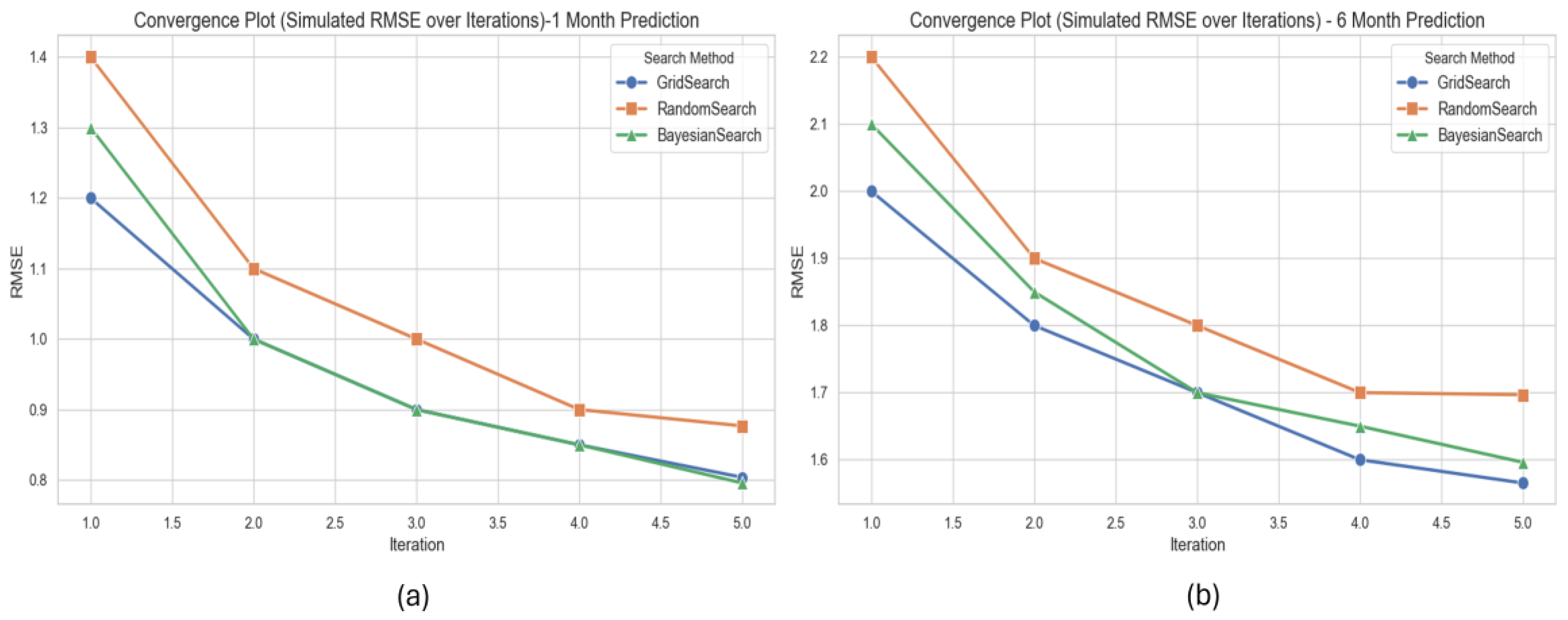
The results of the sensitivity analysis, illustrated in Figure 7, reveal that hyperparameter tuning significantly enhances model performance across all assessed metrics for both short-term (1-month) and long-term (6-month) wind speed forecasting. Each tuning method effectively reduced RMSE, MAE, MAPE, and Max Error compared to the baseline model, underscoring the critical role of systematic optimization in improving both prediction accuracy and model robustness across varying forecast horizons. The convergence behaviors of three hyperparameter tuning strategies, Grid Search, Random Search, and Bayesian Search, are displayed in Figure 8 and are evaluated based on RMSE over successive iterations. The findings indicate that all methods progressively lowered RMSE, signifying enhanced model performance through iterative tuning. Notably, Bayesian optimization demonstrated a faster convergence and achieved the lowest RMSE values in both 1-month and 6-month prediction scenarios, suggesting it is a more efficient and effective search strategy for identifying optimal model parameters in wind speed forecasting tasks.

Based on the combined results from Table 4 and Table 5, it is evident that hyperparameter tuning plays a crucial role in improving the prediction accuracy of the XGBoost model for wind speed forecasting. The default parameters produced the highest errors across all evaluated metrics, indicating suboptimal performance without appropriate tuning. Among the various hyperparameter tuning methods, Grid Search emerged as the most effective approach for the one-month forecasting task, achieving the lowest Mean Absolute Error (MAE), Mean Absolute Percentage Error (MAPE), and Root Mean Square Error (RMSE). Consequently, it was identified as the best model configuration for short-term predictions. The methodical nature of Grid Search facilitated the identification of optimal combinations of hyperparameters, resulting in the most accurate short-term forecasts for wind speed.

In contrast, for the six-month forecasting task, Randomized Search outperformed Grid Search and Bayesian Search. It provided the lowest MAE and MAPE, indicating that Randomized Search was better at capturing the broader trends required for longer-term forecasting. The randomized approach allowed for a more diverse exploration of the hyperparameter space, which appeared beneficial for the extended forecasting horizon.

For one-month forecasting, the Grid Search-XGBoost model is the best choice, as it produced the lowest MAE and MAPE values, thereby providing the highest accuracy. Randomized Search-XGBoost is the most suitable model for six-month forecasting, as it achieved the best overall performance with minimal prediction errors. The differences in performance observed between the one-month and six-month forecasting scenarios illustrate that the effectiveness of various hyperparameter tuning strategies can differ based on the forecasting horizon. The Grid Search method, characterized by its systematic and exhaustive search approach, proved to be most effective in achieving accuracy for short-term forecasts. Conversely, the Randomized Search method, which allows for broader exploration, produced superior results for long-term trend prediction. Thus, selecting the appropriate hyperparameter tuning method depends significantly on the specific forecasting timeframe and the underlying characteristics of the wind speed dataset.

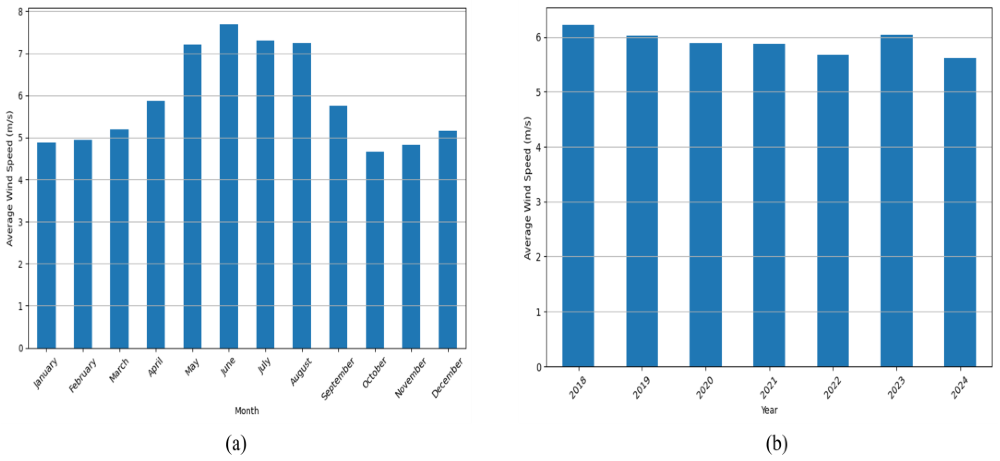
While the absolute differences in MAE values between methods (e.g., 1.224 vs. 1.274) may appear numerically small, they represent statistically significant and operationally meaningful improvements for wind energy forecasting. For context, a 0.05 m/s reduction in MAE can translate to approximately 1.5% better energy yield estimation for a 100 MW wind farm. Furthermore, our tuned models substantially outperform naive baselines (48% better than mean prediction, 25% better than linear regression), demonstrating their practical value. Although average wind speeds during peak months (7–8 m/s) might suggest trivial gains, the proportional impact becomes critical during low-wind seasons (4–5 m/s, Figure 1a), where errors affect grid stability and financial planning more severely. The consistent improvements across MAE, RMSE, and MAPE metrics confirm that our approach captures seasonal and temporal patterns more effectively than simplistic alternatives.

To evaluate the forecasting performance, we compared XGBoost with two baseline models: Mean-based Predictions and Linear Regression. For the one-month ahead predictions, the Mean-based Predictions model produced an MAE of 0.825, MAPE of 13.46%, and RMSE of 1.049. Linear Regression showed improved performance with an MAE of 0.720, MAPE of 11.68%, and RMSE of 0.959, as shown in

Table 6. Evaluation Metric values of Mean-based Predictions and Linear Regression Predictions.

Base_Models	MAE	MAPE	RMSE	CRPS
Mean_based Predictions(1_Month)	0.825	13.46	1.049	0.627
Mean_based Predictions(6_Month)	0.825	13.461	1.049	0.627
Linear Regression Predictions(1_Month)	0.720	11.678	0.959	1.527
Linear Regression Predictions(6_Month)	0.983	17.395	1.158	1.680

. However, both models exhibited significant limitations in longer-term predictions. For six months ahead, Mean-based Predictions remained consistent with the one-month results, indicating its simplicity and inability to capture long-term trends effectively. In contrast, Linear Regression faced a noticeable decline in performance, with MAE increasing to 0.983, MAPE rising to 17.40%, and RMSE increasing to 1.158. XGBoost, however, outperformed both baseline methods in all scenarios, particularly in terms of predictive accuracy. The results from XGBoost (reported separately) demonstrated lower error rates and superior overall performance, highlighting the effectiveness of more sophisticated modeling techniques compared to basic approaches like Mean-based Predictions and Linear Regression. These comparisons confirm the utility of XGBoost in wind speed forecasting, with baseline models serving as a reference for evaluating model improvement

The results indicate that the six-month prediction error values are higher than the one-month prediction. This difference is expected and can be attributed to the increasing forecasting uncertainty over longer time horizons. In short-term predictions, the model benefits from recent wind speed patterns that remain relatively stable, allowing for more accurate forecasts. However, as the forecasting period extends to six months, external factors such as seasonal variations, changing weather patterns, and atmospheric conditions introduce additional complexity. These variations make it more challenging for the model to capture long-term trends accurately, leading to higher error values.

Additionally, time-series forecasting models inherently experience a cumulative effect of prediction errors. Small deviations in earlier predictions can accumulate over time, resulting in larger overall discrepancies in longer forecasts. The increased variability in wind speed over six months further contributes to this effect, as the model faces challenges in capturing long-term dependencies. Despite this, the model remains effective in recognizing overall trends and patterns in the data.

Computational efficiency analysis revealed significant differences in training times across optimization approaches: XGBoost with randomized search completed in 3.8 s, while grid search required 58.0 s, and Bayesian optimization took 1 min 35 s. These results demonstrate that randomized search provides an optimal balance between model performance and computational efficiency, being 15–25× faster than exhaustive search methods while maintaining competitive accuracy. The timing measurements were conducted on OS Windows 10 Pro, OS Type 64-bit operating system, x64-based processor. Processor: Intel(R) Core(TM) i7-4870HQ CPU @ 2.50GHz 2.50 GHz. Graphics NVIDIA, Version 382.05. Installed RAM 16.0 GB under identical experimental conditions.

While the XGBoost model is well suited for both short-term and long-term forecasting, it is natural for prediction accuracy to decrease as the forecasting horizon increases. The increase in error does not indicate a weakness in the model but rather reflects the inherent difficulty of making long-term predictions in dynamic systems such as wind speed forecasting. The observed difference in errors, particularly in the Mean Absolute Error (MAE), aligns with common forecasting challenges where longer-term predictions are associated with greater uncertainty. Nonetheless, the results remain within an acceptable range, demonstrating the model’s robustness in capturing essential trends for practical applications in wind energy management and resource planning.

While this study focused on hyperparameter tuning for the XGBoost model, future work could expand the analysis to include other machine learning models for wind speed forecasting. This would provide a more comprehensive evaluation of the effectiveness of different hyperparameter tuning methods across various models. Additionally, although the hyperparameter tuning methods employed in this study (Grid Search, Random Search, and Bayesian Optimization) are well established, more advanced optimization techniques could further improve the model’s performance. It is also worth noting that the tuned XGBoost model achieved significantly better results compared to baseline models, demonstrating the importance of carefully selecting and optimizing hyperparameters for better prediction accuracy. The MAE increase from 0.51 (1-month) to 1.22 (6-month) aligns with theoretical expectations for multi-step forecasting. While XGBoost struggles with long-term dependencies, its performance remains superior to baseline models (Table 6). Future work could integrate temporal attention mechanisms to mitigate error accumulation.

5. Conclusions

The evaluation of wind speed prediction utilizing the XGBoost model for forecasting horizons of one month and six months emphasizes the critical role of hyperparameter tuning in optimizing the model’s performance. Probabilistic assessment using CRPS further confirmed these findings, demonstrating that tuned models not only improved point forecasts but also provided better-calibrated uncertainty estimates essential for operational decision-making. The default model configuration resulted in the highest prediction errors, indicating that tuning is crucial for improving accuracy. Grid Search and Randomized Search exhibited superior performance relative to the other tuning methods employed in this analysis. Notably, these methods achieved significantly sharper and more reliable predictive distributions, as evidenced by their CRPS values compared to baseline approaches. Specifically, Grid Search was identified as the most effective approach for one-month forecasting, as it achieved the lowest Mean Absolute Error (MAE) and Mean Absolute Percentage Error (MAPE). This advantage extended to probabilistic forecasting, where it produced the most balanced trade-off between precision and uncertainty quantification. In contrast, Randomized Search demonstrated superior performance compared to the other methods for the six-month forecasting task. While all models faced greater uncertainty in long-term predictions, Randomized Search maintained relatively robust probabilistic performance, capturing both central tendencies and extreme value distributions more effectively. These findings indicate that the appropriate hyperparameter tuning strategy depends on the specific forecasting horizon. Grid Search is more effective for short-term accuracy, including probabilistic reliability, while Randomized Search is better suited for long-term trend prediction and uncertainty management. The results highlight the necessity of selecting the tuning method based on the temporal characteristics of the prediction task and the underlying data. However, the XGBoost algorithm has inherent limitations, such as high computational cost, sensitivity to hyperparameters, and challenges in handling long-term dependencies and non-linear trends in time-series data. These limitations also manifest in probabilistic forecasting, where model miscalibration can occur under distribution shifts. Future research should focus on the exploration of advanced optimization techniques and hybrid tuning methodologies to enhance the robustness and generalizability of models, particularly for probabilistic forecasting applications. This is especially pertinent for long-term wind speed forecasting, as it will ultimately contribute to more dependable planning and risk-aware management of renewable energy resources.

References

1. Solarin, S.A.; Bello, M.O. Wind energy and sustainable electricity generation: Evidence from Germany. Environ. Dev. Sustain. 2022, 24, 9185–9198. [Google Scholar] [CrossRef] [PubMed]
2. Mammadov, N.S.; Ganiyeva, N.A.; Aliyeva, G.A. Role of renewable energy sources in the world. J. Renew. Energy Electr. Comput. Eng. 2022, 2, 63–67. [Google Scholar]
3. Krupnov, Y.A.; Krasilnikova, V.G.; Kiselev, V.; Yashchenko, A.V. The contribution of sustainable and clean energy to the strengthening of energy security. Front. Environ. Sci. 2022, 10, 1090110. [Google Scholar] [CrossRef]
4. Pappis, I. Strategic low-cost energy investment opportunities and challenges towards achieving universal electricity access (SDG7) in forty-eight African nations. Environ. Res. Infrastruct. Sustain. 2022, 2, 035005. [Google Scholar] [CrossRef]
5. Mishra, A.; Kumar, R.; Khalkho, A.M.; Mohanta, D.K. An IoT Integrated Reliability Estimation of Wind Energy System. In Proceedings of the 2022 International Conference on IoT and Blockchain Technology (ICIBT), Ranchi, India, 6–8 May 2022; pp. 1–5. [Google Scholar]
6. Kuşkaya, S.; Aldieri, L.; Sharma, G.D.; Balsalobre-Lorente, D. Wind and solar energy sources: Policy, economics, and impacts on environmental quality. Front. Environ. Sci. 2022, 10, 1054259. [Google Scholar] [CrossRef]
7. Miele, E.S.; Ludwig, N.; Corsini, A. Multi-horizon wind power forecasting using multi-modal spatio-temporal neural networks. Energies 2023, 16, 3522. [Google Scholar] [CrossRef]
8. Rodriguez, H.; Flores, J.J.; Morales, L.A.; Lara, C.; Guerra, A.; Manjarrez, G. Forecasting from incomplete and chaotic wind speed data. Soft Comput. 2019, 23, 10119–10127. [Google Scholar] [CrossRef]
9. Guo, T.; Zhang, L.; Liu, Z.; Wang, J. A combined strategy for wind speed forecasting using data preprocessing and weight coefficients optimization calculation. IEEE Access 2020, 8, 33039–33059. [Google Scholar] [CrossRef]
10. Cruz, J.C.; Oliveira, D.Q.; Neto, F.A.; do Monte, L.T.D.A. Analysis of a Wind Speed Prediction Model Based on Decision Trees. In Proceedings of the 2023 Workshop on Communication Networks and Power Systems (WCNPS), Brasilia, Brazil, 30 November–1 December 2023; pp. 1–7. [Google Scholar]
11. Clare, M.C.; Warder, S.C.; Neal, R.; Bhaskaran, B.; Piggott, M.D. An unsupervised learning approach for predicting wind farm power and downstream wakes using weather patterns. arXiv 2023, arXiv:2302.05886. [Google Scholar] [CrossRef]
12. Cheneka, B.R.; Watson, S.J.; Basu, S. Quantifying the impacts of synoptic weather patterns on North Sea wind power production and ramp events under a changing climate. Energy Clim. Chang. 2023, 4, 100113. [Google Scholar] [CrossRef]
13. Shen, Z.; Fan, X.; Zhang, L.; Yu, H. Wind speed prediction of unmanned sailboat based on CNN and LSTM hybrid neural network. Ocean Eng. 2022, 254, 111352. [Google Scholar] [CrossRef]
14. Yang, Q.; Huang, G.; Li, T.; Xu, Y.; Pan, J. A novel short-term wind speed prediction method based on hybrid statistical-artificial intelligence model with empirical wavelet transform and hyperparameter optimization. J. Wind Eng. Ind. Aerodyn. 2023, 240, 105499. [Google Scholar] [CrossRef]
15. Liu, Y.; Zhang, Z.; Huang, Y.; Zhao, W.; Dai, L. Hybrid neural network-aided strong wind speed prediction along rail network. J. Wind Eng. Ind. Aerodyn. 2024, 252, 105813. [Google Scholar] [CrossRef]
16. Liu, M.D.; Ding, L.; Bai, Y.L. Application of hybrid model based on empirical mode decomposition, novel recurrent neural networks and the ARIMA to wind speed prediction. Energy Convers. Manag. 2021, 233, 113917. [Google Scholar] [CrossRef]
17. Han, Y.; Mi, L.; Shen, L.; Cai, C.S.; Liu, Y.; Li, K.; Xu, G. A short-term wind speed prediction method utilizing novel hybrid deep learning algorithms to correct numerical weather forecasting. Appl. Energy 2022, 312, 118777. [Google Scholar] [CrossRef]
18. Li, J.; Song, Z.; Wang, X.; Wang, Y.; Jia, Y. A novel offshore wind farm typhoon wind speed prediction model based on PSO–Bi-LSTM improved by VMD. Energy 2022, 251, 123848. [Google Scholar] [CrossRef]
19. Lv, S.X.; Wang, L. Multivariate wind speed forecasting based on multi-objective feature selection approach and hybrid deep learning model. Energy 2023, 263, 126100. [Google Scholar] [CrossRef]
20. Suo, L.; Peng, T.; Song, S.; Zhang, C.; Wang, Y.; Fu, Y.; Nazir, M.S. Wind speed prediction by a swarm intelligence based deep learning model via signal decomposition and parameter optimization using improved chimp optimization algorithm. Energy 2023, 276, 127526. [Google Scholar] [CrossRef]
21. Zhang, C.; Li, Z.; Ge, Y.; Liu, Q.; Suo, L.; Song, S.; Peng, T. Enhancing short-term wind speed prediction based on an outlier-robust ensemble deep random vector functional link network with AOA-optimized VMD. Energy 2024, 296, 131173. [Google Scholar] [CrossRef]
22. Sun, X.; Liu, H. Multivariate short-term wind speed prediction based on PSO-VMD-SE-ICEEMDAN two-stage decomposition and Att-S2S. Energy 2024, 305, 132228. [Google Scholar] [CrossRef]
23. Barjasteh, A.; Ghafouri, S.H.; Hashemi, M. A hybrid model based on discrete wavelet transform (DWT) and bidirectional recurrent neural networks for wind speed prediction. Eng. Appl. Artif. Intell. 2024, 127, 107340. [Google Scholar] [CrossRef]
24. Shi, Z.; Li, J.; Jiang, Z.; Li, H.; Yu, C.; Mi, X. WGformer: A Weibull-Gaussian Informer based model for wind speed prediction. Eng. Appl. Artif. Intell. 2024, 131, 107891. [Google Scholar] [CrossRef]
25. Wang, Y.; Yang, P.; Zhao, S.; Chevallier, J.; Xiao, Q. A hybrid intelligent framework for forecasting short-term hourly wind speed based on machine learning. Expert Syst. Appl. 2023, 213, 119223. [Google Scholar] [CrossRef]
26. Wu, Q.; Zheng, H.; Guo, X.; Liu, G. Promoting wind energy for sustainable development by precise wind speed prediction based on graph neural networks. Renew. Energy 2022, 199, 977–992. [Google Scholar] [CrossRef]
27. Wang, Z.; Wang, L.; Revanesh, M.; Huang, C.; Luo, X. Short-term wind speed and power forecasting for smart city power grid with a hybrid machine learning framework. IEEE Internet Things J. 2023, 10, 18754–18765. [Google Scholar] [CrossRef]
28. Subbiah, S.S.; Paramasivan, S.K.; Arockiasamy, K.; Senthivel, S.; Thangavel, M. Deep Learning for Wind Speed Forecasting Using Bi-LSTM with Selected Features. Intell. Autom. Soft Comput. 2023, 35, 3829–3844. [Google Scholar] [CrossRef]
29. Pun, K.; Basnet, S.M.; Jewell, W. Wind Power Prediction in Different Months of the Year Using Machine Learning Techniques. In Proceedings of the 2021 IEEE Kansas Power and Energy Conference (KPEC), Manhattan, KS, USA, 19–20 April 2021; pp. 1–6. [Google Scholar]
30. Lydia, M.; Edwin Prem Kumar, G.; Akash, R. Wind speed and wind power forecasting models. Energy Environ. 2024. [Google Scholar] [CrossRef]
31. Zhang, Y.; Hiraga, Y.; Campus, T.D.A. Review of Recent Advances in Long-Term Wind Speed and Power Forecasting. ESS Open Arch. Eprints 2024, 124, 12431386. [Google Scholar]
32. Shouman, E.R.M. Wind Power Forecasting Models. In Wind Turbines-Advances and Challenges in Design, Manufacture and Operation; IntechOpen: Rijeka, Croatia, 2022. [Google Scholar]
33. Gneiting, T.; Katzfuss, M. Probabilistic forecasting. Annu. Rev. Stat. Its Appl. 2014, 1, 125–151. [Google Scholar] [CrossRef]
34. Hersbach, H. Decomposition of the continuous ranked probability score for ensemble prediction systems. Weather Forecast. 2000, 15, 559–570. [Google Scholar] [CrossRef]
35. Dowell, J.; Pinson, P. Very-short-term probabilistic wind power forecasts by sparse vector autoregression. IEEE Trans. Smart Grid 2015, 7, 763–770. [Google Scholar] [CrossRef]
36. Bashar, T.R.; Munem, M.; Islam, M.S.; Hossain, M.; Shawkat, T.B.; Rahaman, H. Optimized hybrid neural network for wind speed forecasting. In Proceedings of the 2022 IEEE Electrical Power and Energy Conference (EPEC), Victoria, BC, Canada, 5–7 December 2022; pp. 284–289. [Google Scholar]
37. Kumar, R.; Prakash, M.; Shakila, B. A comparative analysis of time series and machine learning models for wind speed prediction. In Proceedings of the 2023 IEEE 3rd Mysore Sub Section International Conference (MysuruCon), HASSAN, India, 1–2 December 2023; pp. 1–6. [Google Scholar]
38. Das, N.; Deb, S.; Goswami, A.K. Day-ahead Wind Power Prediction using Optimised XGBoost and Correlation Analysis based Noise Reduction Technique. In Proceedings of the 2022 IEEE International Conference on Power Electronics, Drives and Energy Systems (PEDES), Jaipur, India, 14–17 December 2022; pp. 1–6. [Google Scholar]
39. Xiong, X.; Guo, X.; Zeng, P.; Zou, R.; Wang, X. A short-term wind power forecast method via XGBoost hyper-parameters optimization. Front. Energy Res. 2022, 10, 905155. [Google Scholar] [CrossRef]
40. Dong, D.; Wen, F.; Zhang, Y.; Qiu, W. Application of XGboost in electricity consumption prediction. In Proceedings of the 2023 IEEE 3rd International Conference on Electronic Technology, Communication and Information (ICETCI), Changchun, China, 26–28 May 2023; pp. 1260–1264. [Google Scholar]
41. Bao, Y.; Liu, Z. A fast grid search method in support vector regression forecasting time series. In Intelligent Data Engineering and Automated Learning–IDEAL 2006, Proceedings of the 7th International Conference, Burgos, Spain, 20–23 September 2006; Proceedings 7; Springer: Berlin/Heidelberg, Germany, 2006; pp. 504–511. [Google Scholar]
42. Montanari, M.; Bernardis, C.; Cremonesi, P. On the impact of data sampling on hyper-parameter optimisation of recommendation algorithms. In Proceedings of the 37th ACM/SIGAPP Symposium on Applied Computing, Virtual, 25–29 April 2022; pp. 1399–1402. [Google Scholar]
43. Turner, R.; Eriksson, D.; McCourt, M.; Kiili, J.; Laaksonen, E.; Xu, Z.; Guyon, I. Bayesian optimization is superior to random search for machine learning hyperparameter tuning: Analysis of the black-box optimization challenge 2020. In Proceedings of the NeurIPS 2020 Competition and Demonstration Track, Virtual, 6–12 December 2020. [Google Scholar]
44. Andrade, J.R.; Bessa, R.J. Improving renewable energy forecasting with a grid of numerical weather predictions. IEEE Trans. Sustain. Energy 2017, 8, 1571–1580. [Google Scholar] [CrossRef]
45. Memon, S.A.; Javed, Q.; Kim, W.-G.; Mahmood, Z.; Khan, U.; Shahzad, M. A Machine-Learning-Based Robust Classification Method for PV Panel Faults. Sensors 2022, 22, 8515. [Google Scholar] [CrossRef]
46. Montiel, J.; Mitchell, R.; Frank, E.; Pfahringer, B.; Abdessalem, T.; Bifet, A. Adaptive xgboost for evolving data streams. In Proceedings of the 2020 International Joint Conference on Neural Networks (IJCNN), Glasgow, UK, 19–24 July 2020; pp. 1–8. [Google Scholar]
47. Mienye, I.D.; Sun, Y. A survey of ensemble learning: Concepts, algorithms, applications, and prospects. IEEE Access 2022, 10, 99129–99149. [Google Scholar] [CrossRef]
Figure 1. (a) Average monthly wind speed from 2018 to July 2024. (b) Average annual wind speed from July 2018 to July 2024.
Processes 13 01763 g001
Figure 2. Wind speed trends with peak seasonal activity (2018–2024).
Processes 13 01763 g002
Figure 3. Overview of the Data Preprocessing and Evaluation Framework.
Processes 13 01763 g003
Figure 4. Proposed framework integrating XGBoost for monthly wind speed forecasting with the architectural flow of the XGBoost algorithm.
Processes 13 01763 g004
Figure 5. Historical and Forecasted Wind Speeds with Confidence Intervals.
Processes 13 01763 g005
Figure 6. Relationship between actual and predicted wind speeds for an XGBoost.
Processes 13 01763 g006
Figure 7. Sensitivity analysis of wind speed prediction performance: (a) one-month forecast, (b) six-month forecast.
Processes 13 01763 g007
Figure 8. Convergence analysis showing RMSE reduction over iterations for different hyperparameter optimization methods: (a) for 1-month (b) for 6-month predictions.
Processes 13 01763 g008