
Load Frequency Control via Multi-Agent Reinforcement Learning and Consistency Model for Diverse Demand-Side Flexible Resources

Abstract
1. Introduction
- A universal model incorporating power constraints, energy constraints, and first-order inertia characteristics is constructed, using only a few key parameters to characterize resource response delays and dynamic behaviors.
- A policy gradient controller is designed to guide the update of agent network parameters by combining frequency deviations and resource response characteristics. Through projected gradient descent, the parameter update direction is adjusted to the tangent direction of the feasible domain, ensuring that actions always satisfy constraints.
- A novel reward function for frequency control is proposed, dynamically adjusting weight factors and penalty terms based on resource states to achieve a priority configuration for different optimization objectives.
2. A Consistency Model for Frequency Control Involving Diverse Flexible Resources
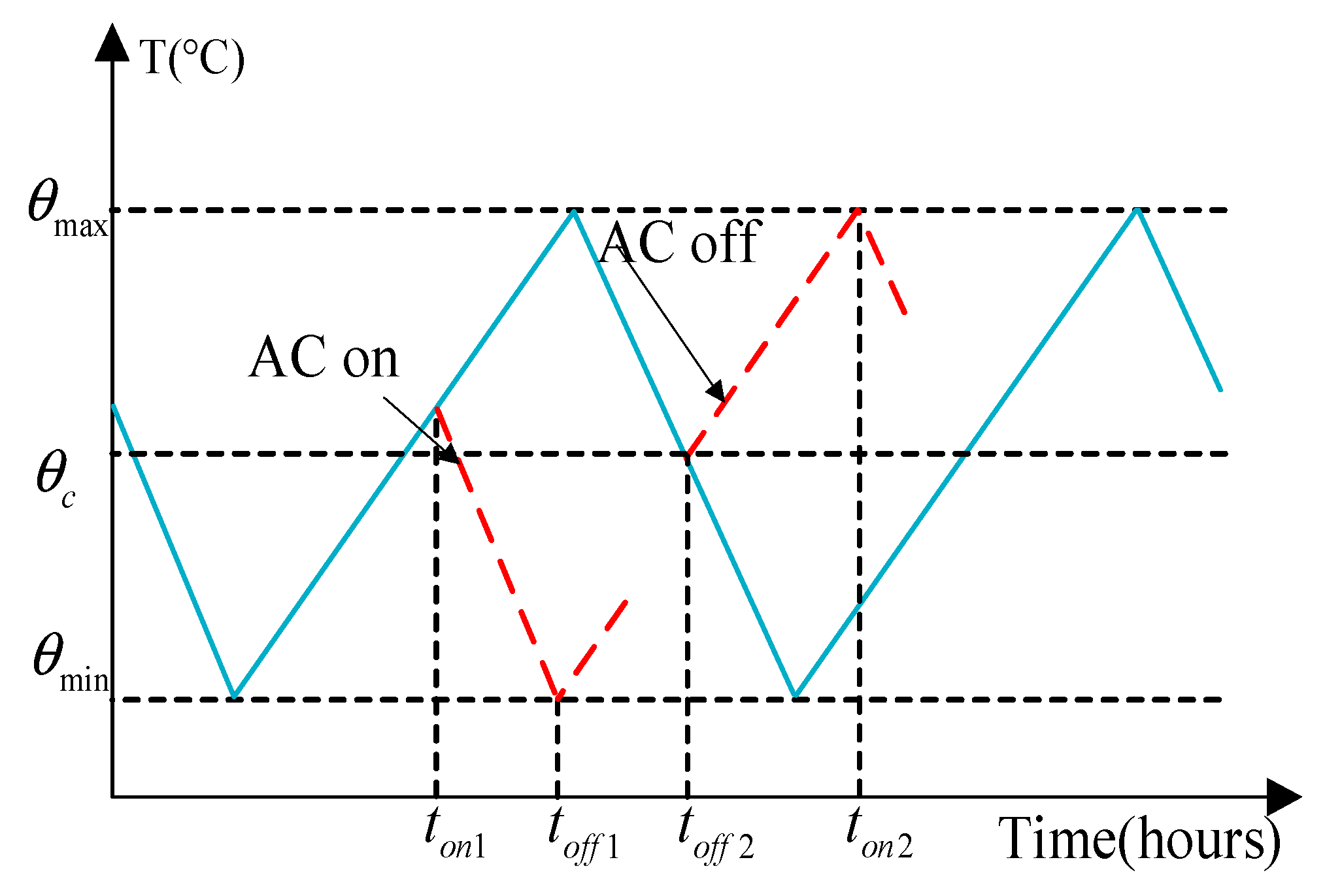
2.1. Consistency Model for Air Conditioning Loads
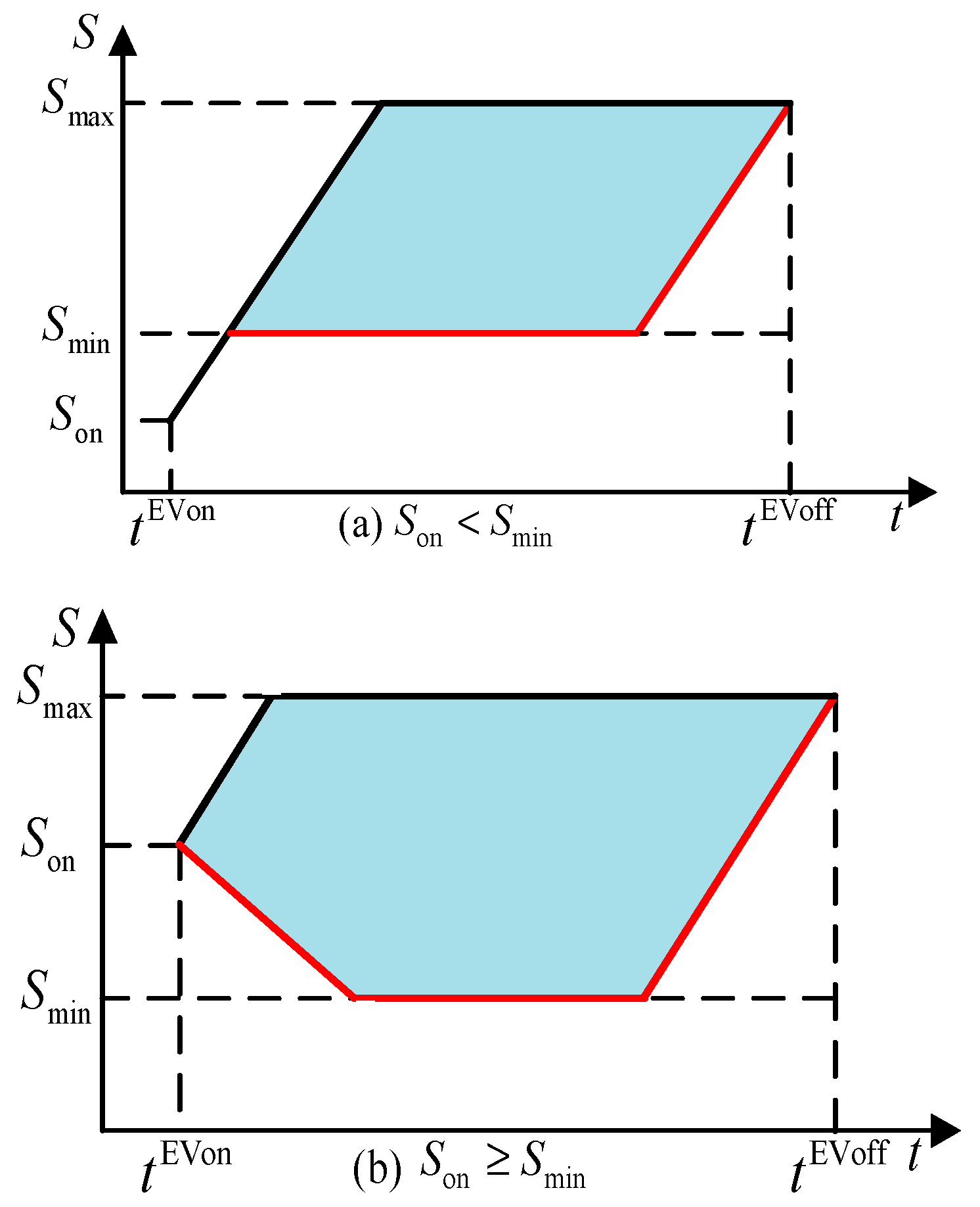
2.2. Consistency Model for Electric Vehicles
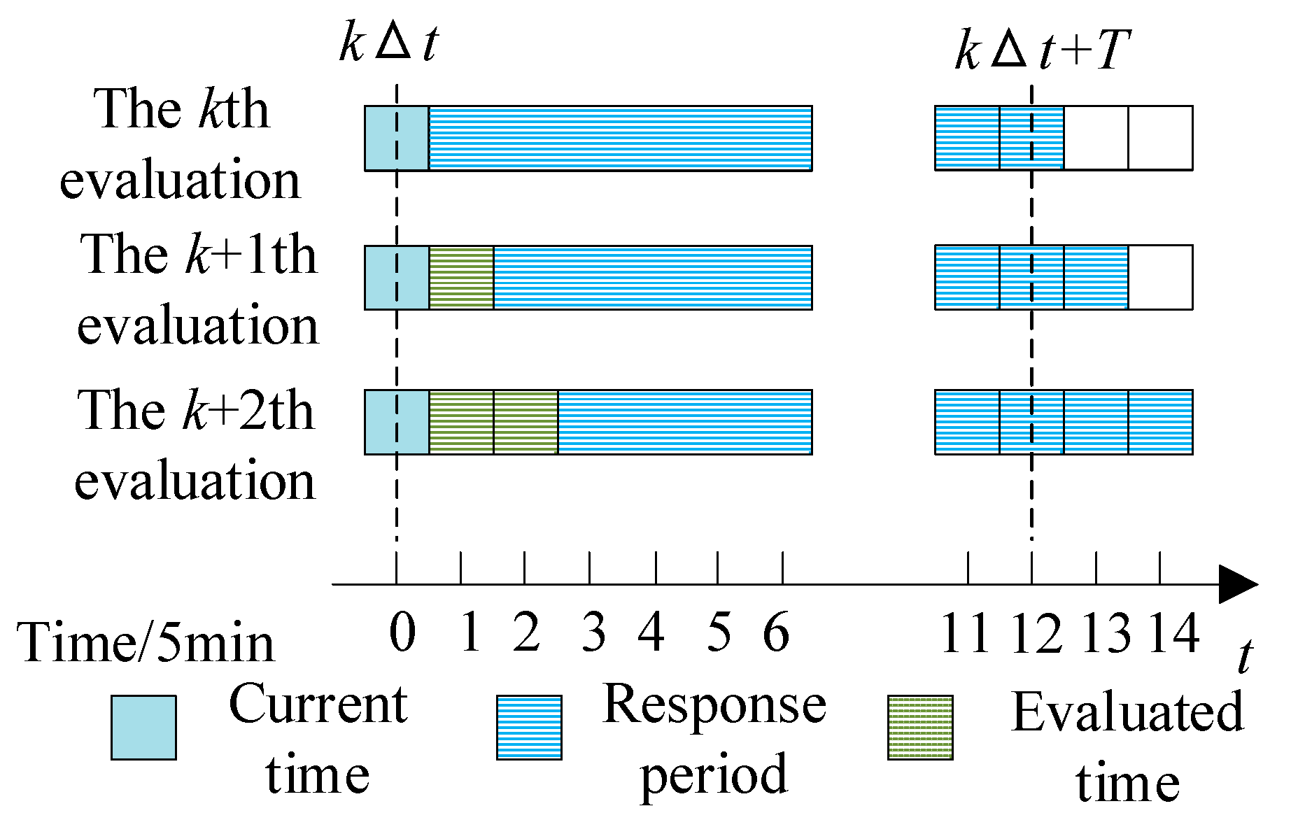
2.3. Assessing the Controllable Potential Considering the Uncertainty of Flexible Resources
- For flexible resources newly connected to the grid during the response period, if the demand-side flexible resources can reach the minimum power capacity at the end of the response period, the lower limit of the FM power potential of the flexible resources will be corrected:
- 2.
- Similar to the earlier addressed scenario for the recently grid-connected flexible resources, the frequency regulation capability of the remaining period should be re-evaluated for flexible resources with a delayed off-grid time if the CM has reached the set electrical energy. If the CM has not reached the set electrical energy, the upper and lower limits of the frequency regulation power of the flexible resources should be revised to the allowable maximum charging power.
- 3.
- For the flexible resources that go off-grid in advance, the upper and lower limits of their frequency regulation power should be revised to zero, and they will not participate in the frequency response for the remaining time.
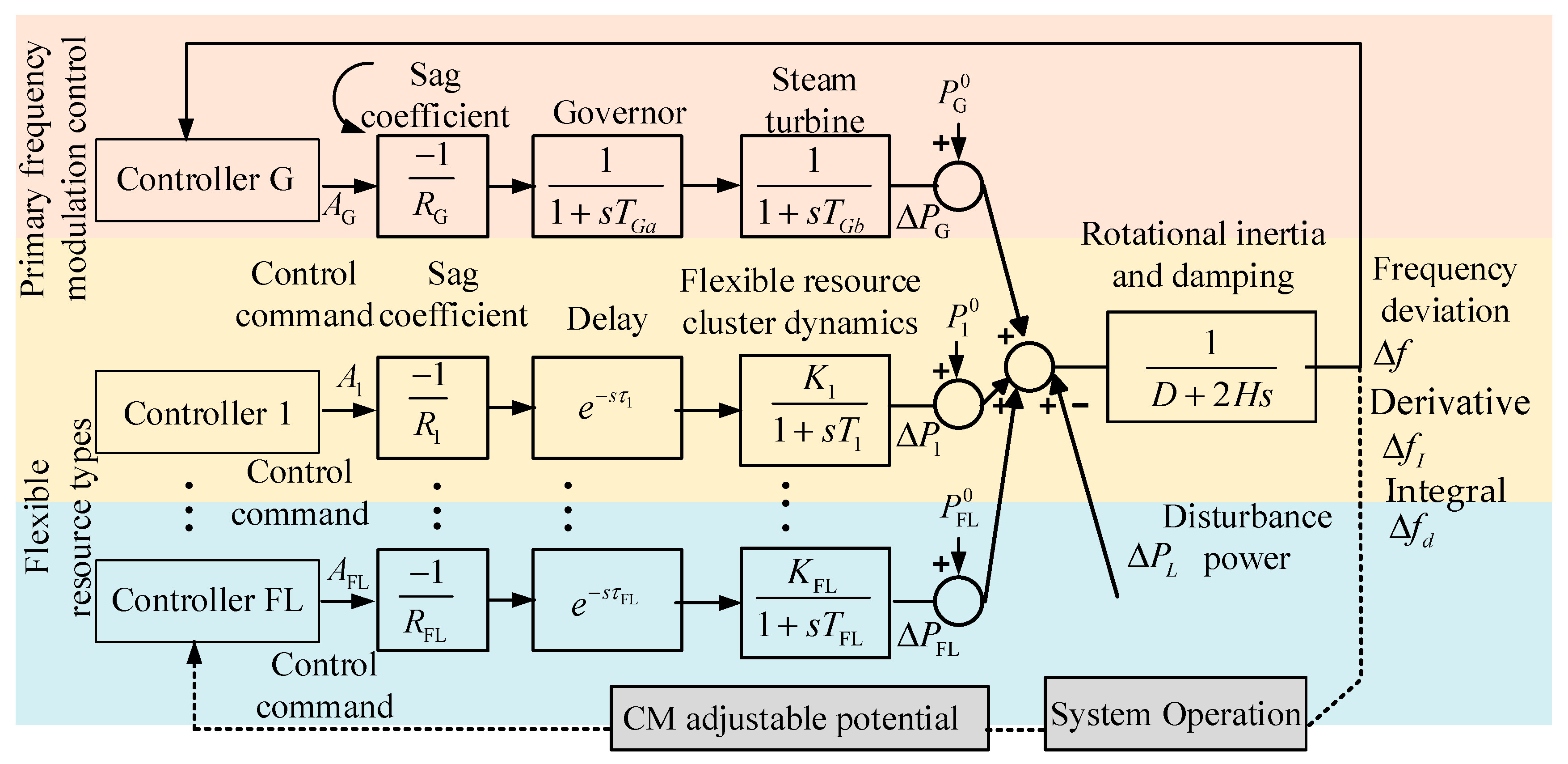
2.4. Consistency Model Considering the Participation of Different Types of Resources in Frequency Control
3. Proposed Method
3.1. Control Objectives and Reward Functions
3.2. Actor Network Parameter Update Method
4. System Studies
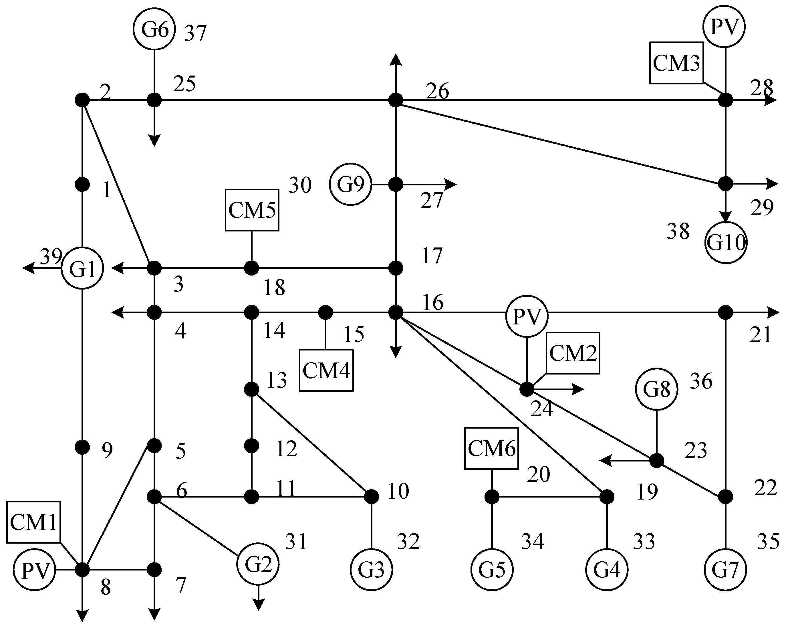
4.1. Test System
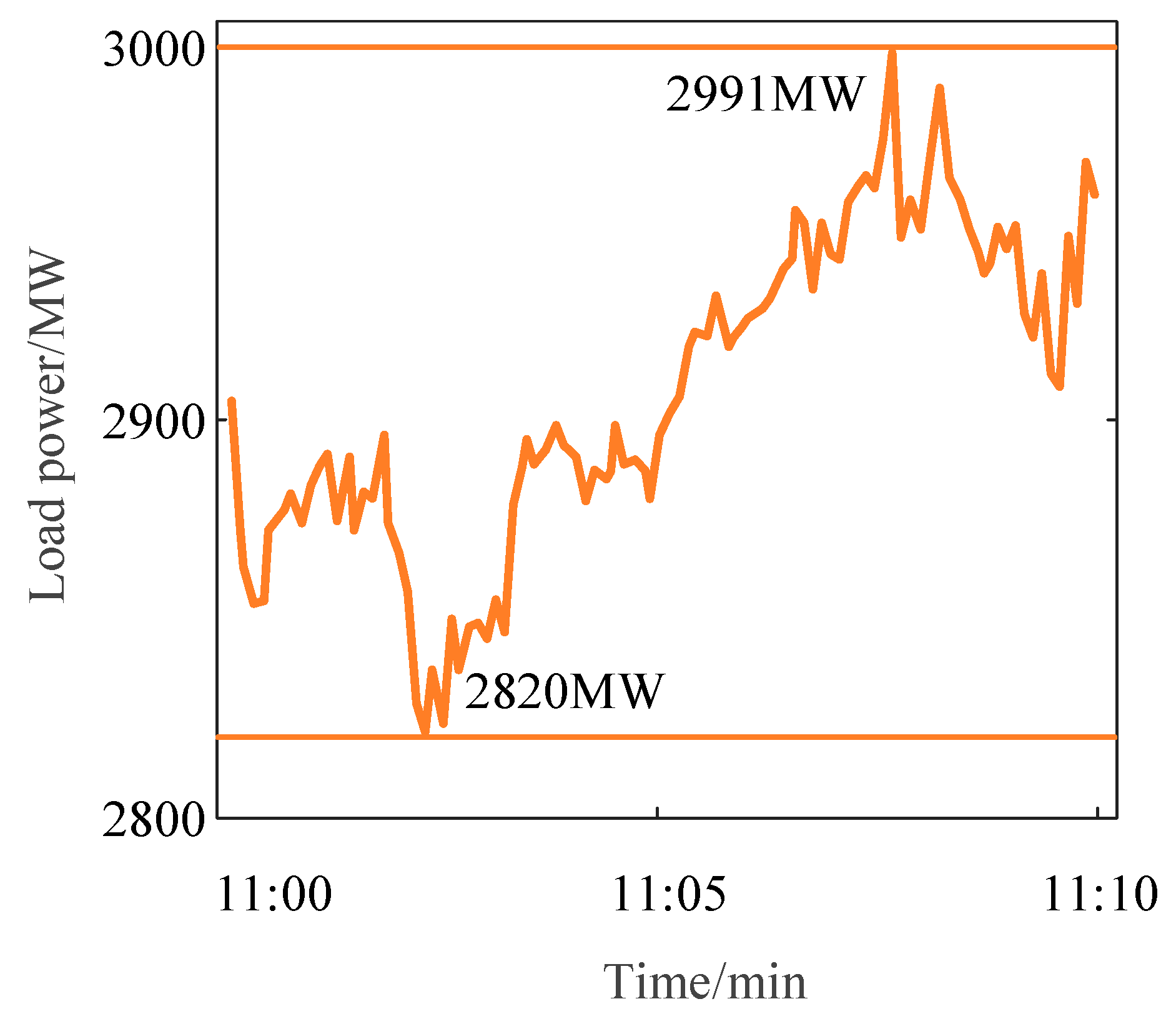
4.2. System Random and Load Perturbation
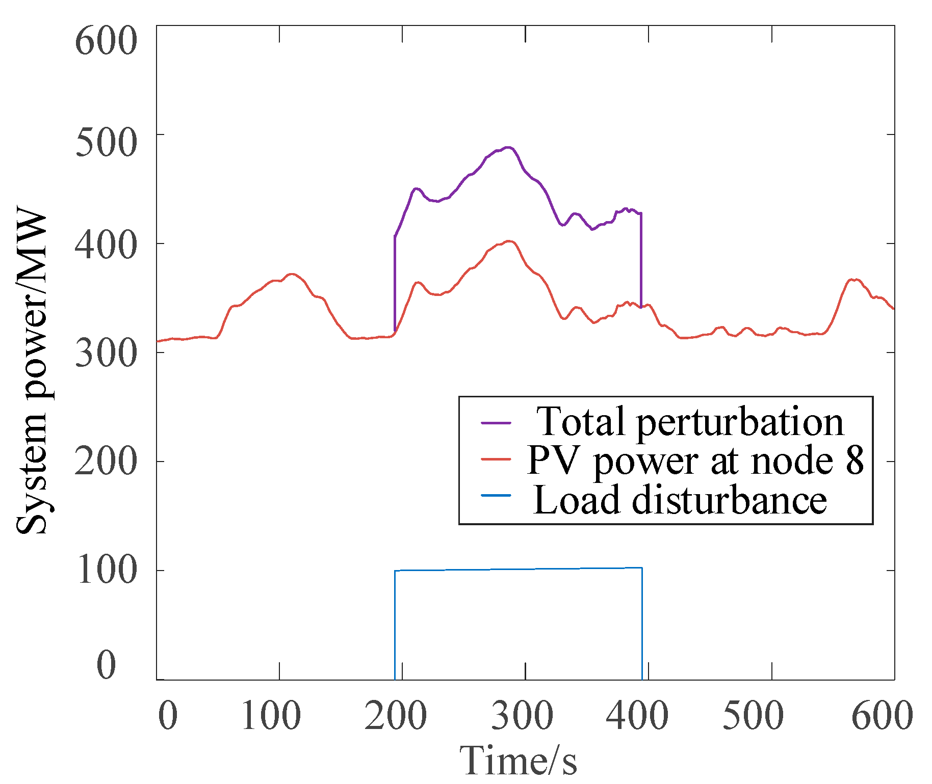
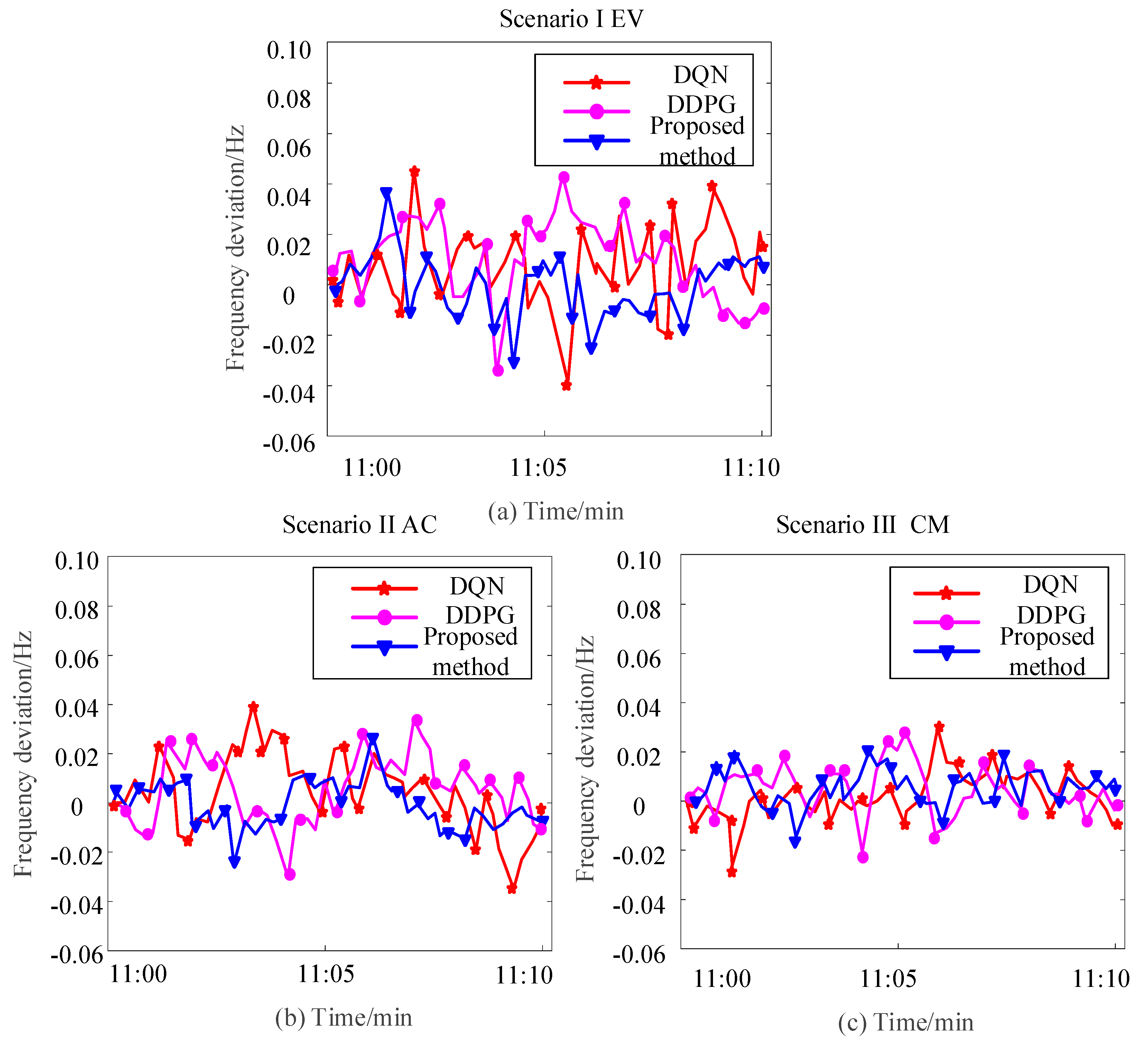
4.3. High Percentage of New Energy Disturbances
5. Conclusions
Author Contributions
Funding
Data Availability Statement
Conflicts of Interest
Nomenclature
| Variables | |
| The thermal inertia coefficient | |
| The building’s equivalent thermal resistance | |
| The equivalent thermal capacitance | |
| The energy efficiency coefficient | |
| The ACs power consumption | |
| The ambient temperature | |
| The interior temperature | |
| The binary on/off state | |
| The ACs setpoint temperature | |
| The dead band width | |
| The baseline charging/discharging power | |
| The energy state of ACs at time t | |
| The time step duration | |
| The maximum power limits | |
| The minimum power limits | |
| The energy state of the ACs cluster CM | |
| The power state of the ACs cluster CM | |
| Maximum energy state boundaries | |
| Minimum energy state boundaries | |
| The charging/discharging power of the ACs cluster | |
| The charge/discharge time constant of the ACs cluster | |
| The droop control parameter of the ACs cluster | |
| The time delay of ACs | |
| Laplace variable | |
| Reference droop control coefficients for ACs | |
| Reference droop control coefficients for EVs | |
| Set the value of the state of charge of flexible resources | |
| The state of charge of flexible resources | |
| Reference droop control coefficient of flexible resources | |
| The grid-connection time of EVs | |
| The grid-disconnection time | |
| The maximum energy states of the EVs at time t | |
| The minimum energy states of the EVs at time t | |
| The maximum charging and discharging power of the i-th EVs | |
| The minimum charging and discharging power of the i-th EVs | |
| The minimum energy thresholds at grid connection | |
| The minimum energy thresholds at disconnection times | |
| The initial energy state of the i-th EVs | |
| The required energy state of the i-th EVs | |
| The number of EV clusters | |
| The grid-connected status of the i-th vehicle | |
| The upper and lower limits of the electrical energy of the EV cluster CM | |
| The upper and lower limits of the power of the EV cluster CM | |
| The energy state of the EV cluster’s CM | |
| The power of the EV cluster’s CM | |
| The charging/discharging power of the EV cluster | |
| The charge/discharge time constant of the EV cluster | |
| The droop control parameter of the EV cluster | |
| The time delay of EVs | |
| The current moment | |
| The moment when the response ends | |
| The minimum charging amount or the maximum discharging amount of the flexible resource | |
| The electrical energy of the flexible resource | |
| The charging and discharging efficiencies | |
| The charging and discharging efficiencies | |
| The set value of the state of charge when the flexible resource is off-grid | |
| The set off-grid moment | |
| The maximum charging and discharging power | |
| The lower limit of the frequency regulation power within the response period | |
| The allowable increase in the electrical energy | |
| The upper limit of the frequency regulation power within the response period | |
| The droop control coefficient | |
| The time constants of the speed governor | |
| The steam turbine | |
| The governor steam turbine dynamic | |
| The sag control parameters | |
| The time constant | |
| The time delay link of the different flexible resource clusters | |
| The delay time constant of the different flexible resource clusters | |
| The power output of different flexibility resources | |
| The CM power output | |
| Frequency deviation | |
| The derivative of the deviation | |
| The integral of the deviation | |
| The reference operating points of the flexible resource | |
| The reference operating points of the generator | |
| Controller Output | |
| The power variation of the j-th flexible resource cluster | |
| The number of frequency regulation units | |
| The number of flexible resource clusters | |
| The power variations of the i-th frequency regulation unit | |
| The disturbance power | |
| The system’s inertia time constant | |
| Load damping coefficient | |
| The action policy | |
| The policy network | |
| State | |
| The action value function | |
| The neural network parameters | |
| The dimensionally unified outputs | |
| The unit power output cost of the generator | |
| The unit power output cost of the flexible resource cluster | |
| The weighting coefficient | |
| The reward function | |
| Discount factor | |
| Weight coefficient | |
| Weight coefficient | |
| Weight coefficient | |
| The change in the power reference value | |
| The state of charge | |
| The set value of the state of charge | |
| The expected state-action value function | |
| The learning rate | |
| The activation function | |
| The number of layers of the neural network | |
| The datum values | |
| The base operating point | |
| The minimum output power constraint | |
| The maximum output power constraint | |
| Absolute frequency deviation | |
| Training time | |
| Decision time | |
| Average FM costs | |
| Abbreviations | |
| DSFRs | Demand-side flexible resources |
| EVs | Electric vehicles |
| CM | Consistency Model |
| ACs | Air conditioners |
| FM | Frequency modulation |
| DRL | Deep reinforcement learning |
| PV | Photovoltaic |
| DQN | Deep Q-network |
| DDPG | Deep deterministic policy gradient |
| LFC | Load frequency control |
References
- Fang, J.; Li, H.; Tang, Y.; Blaabjerg, F. On the Inertia of Future More-Electronics Power Systems. IEEE J. Emerg. Sel. Top. Power Electron. 2019, 7, 2130–2146. [Google Scholar] [CrossRef]
- Hu, P.; Li, Y.; Yu, Y.; Blaabjerg, F. Inertia estimation of renewable-energy-dominated power system. Renew. Sustain. Energy Rev. 2023, 183, 113481. [Google Scholar] [CrossRef]
- Moore, P.; Alimi, O.A.; Abu-Siada, A. A Review of System Strength and Inertia in Renewable-Energy-Dominated Grids: Challenges, Sustainability, and Solutions. Challenges 2025, 16, 12. [Google Scholar] [CrossRef]
- Yu, G.; Liu, C.; Tang, B.; Chen, R.; Lu, L.; Cui, C.; Hu, Y.; Shen, L.; Muyeen, S.M. Short term wind power prediction for regional wind farms based on spatial-temporal characteristic distribution. Renew. Energy 2022, 199, 599–612. [Google Scholar] [CrossRef]
- Yu, G.Z.; Lu, L.; Tang, B.; Wang, S.Y.; Chen, R.S.; Chung, C.Y. Ultra-short-term Wind Power Subsection Forecasting Method Based on Extreme Weather. IEEE Trans. Power Syst. 2022, 38, 5045–5056. [Google Scholar] [CrossRef]
- Azizi, S.; Sun, M.; Liu, G.; Terzija, V. Local Frequency-Based Estimation of the Rate of Change of Frequency of the Center of Inertia. IEEE Trans. Power Syst. 2020, 35, 4948–4951. [Google Scholar] [CrossRef]
- Liu, X.; Liu, Y.; Liu, J.; Xiang, Y.; Yuan, X. Optimal planning of AC-DC hybrid transmission and distributed energy resource system: Review and prospects. CSEE J. Power Energy Syst. 2019, 5, 409–422. [Google Scholar] [CrossRef]
- Shrivastava, S.; Khalid, S.; Nishad, D.K. Impact of EV interfacing on peak-shelving and frequency regulation in a microgrid. Sci. Rep. 2024, 14, 31514. [Google Scholar] [CrossRef]
- Zhao, H.; Wu, Q.; Huang, S.; Zhang, H.; Liu, Y.; Xue, Y. Hierarchical control of thermostatically controlled loads for primary frequency support. IEEE Trans. Smart Grid 2018, 9, 2986–2998. [Google Scholar] [CrossRef]
- Jendoubi, I.; Sheshyekani, K.; Dagdougui, H. Aggregation and optimal management of TCLs for frequency and voltage control of a microgrid. IEEE Trans. Power Deliv. 2021, 36, 2085–2096. [Google Scholar] [CrossRef]
- Yu, Z.; Bao, Y.; Yang, X. Day-ahead scheduling of air-conditioners based on equivalent energy storage model under temperature-set-point control. Appl. Energy 2024, 368, 123481. [Google Scholar] [CrossRef]
- Cai, L.; Yang, C.; Li, J.; Liu, Y.; Yan, J.; Zou, X. Study on Frequency-Response Optimization of Electric Vehicle Participation in Energy Storage Considering the Strong Uncertainty Model. World Electr. Veh. J. 2025, 16, 35. [Google Scholar] [CrossRef]
- Shukla; Rajan, R.; Garg, M.M.; Panda, A.K. Driving grid stability: Integrating electric vehicles and energy storage devices for efficient load frequency control in isolated hybrid microgrids. J. Energy Storage 2024, 89, 111654. [Google Scholar] [CrossRef]
- Wen, Y.; Hu, Z.; You, S.; Duan, X. Aggregate Feasible Region of DERs: Exact Formulation and Approximate Models. IEEE Trans. Smart Grid 2022, 13, 4405–4423. [Google Scholar] [CrossRef]
- Wang, S.; Wu, W. Aggregate Flexibility of Virtual Power Plants with Temporal Coupling Constraints. IEEE Trans. Smart Grid 2021, 12, 5043–5051. [Google Scholar] [CrossRef]
- Feng, C.; Chen, Q.; Wang, Y.; Kong, P.Y.; Gao, H.; Chen, S. Provision of Contingency Frequency Services for Virtual Power Plants with Aggregated Models. IEEE Trans. Smart Grid 2023, 14, 2798–2811. [Google Scholar] [CrossRef]
- Huang, X.; Li, K.; Xie, Y.; Liu, B.; Liu, J.; Liu, Z.; Mou, L. A novel multistage constant compressor speed control strategy of electric vehicle air conditioning system based on genetic algorithm. Energy 2022, 241, 122903. [Google Scholar] [CrossRef]
- Liu, W.; Tan, J.; Cui, J. Design of a PID Control Scheme for Pound-Drever–Hall Frequency-Tracking System Based on System Identification and Fuzzy Control. IEEE Sens. J. 2024, 24, 39252–39259. [Google Scholar] [CrossRef]
- He, L.; Tan, Z.; Li, Y.; Cao, Y.; Chen, C. A Coordinated Consensus Control Strategy for Distributed Battery Energy Storages Considering Different Frequency Control Demands. IEEE Trans. Sustain. Energy 2024, 15, 304–315. [Google Scholar] [CrossRef]
- Xie, J.; Sun, W. Distributional Deep Reinforcement Learning-Based Emergency Frequency Control. IEEE Trans. Power Syst. 2022, 37, 2720–2730. [Google Scholar] [CrossRef]
- Li, J.; Yu, T.; Cui, H. A multi-agent deep reinforcement learning-based “Octopus” cooperative load frequency control for an interconnected grid with various renewable units. Sustain. Energy Technol. Assess. 2022, 51, 101899. [Google Scholar] [CrossRef]
- Chen, X.; Zhang, M.; Wu, Z.; Wu, L.; Guan, X. Model-Free Load Frequency Control of Nonlinear Power Systems Based on Deep Reinforcement Learning. IEEE Trans. Ind. Inform. 2024, 20, 6825–6833. [Google Scholar] [CrossRef]
- Yu, L.; Sun, Y.; Xu, Z.; Shen, C.; Yue, D.; Jiang, T.; Guan, X. Multi-agent deep reinforcement learning for HVAC control in commercial buildings. IEEE Trans. Smart Grid 2021, 12, 407–419. [Google Scholar] [CrossRef]
- Sahu, P.C.; Baliarsingh, R.; Prusty, R.C.; Panda, S. Novel DQN optimised tilt fuzzy cascade controller for frequency stability of a tidal energy-based AC microgrid. Int. J. Ambient. Energy 2020, 43, 3587–3599. [Google Scholar] [CrossRef]
- Li, J.; Zhou, T. Prior Knowledge Incorporated Large-Scale Multiagent Deep Reinforcement Learning for Load Frequency Control of Isolated Microgrid Considering Multi-Structure Coordination. IEEE Trans. Ind. Inform. 2024, 20, 3923–3934. [Google Scholar] [CrossRef]
- Lee, W.-G.; Kim, H.-M. Deep Reinforcement Learning-Based Dynamic Droop Control Strategy for Real-Time Optimal Operation and Frequency Regulation. IEEE Trans. Sustain. Energy 2025, 16, 284–294. [Google Scholar] [CrossRef]
- Dobbe, R.; Hidalgo-Gonzalez, P.; Karagiannopoulos, S.; Henriquez-Auba, R.; Hug, G.; Callaway, D.S.; Tomlin, C.J. Learning to control in power systems: Design and analysis guidelines for concrete safety problems. Electr. Power Syst. Res. 2020, 189, 106615. [Google Scholar] [CrossRef]
- Zhang, Z.; Zhang, D.; Qiu, R.C. Deep reinforcement learning for power system applications: An overview. CSEE J. Power Energy Syst. 2019, 6, 213–225. [Google Scholar]
- Hao, H.; Somani, A.; Lian, J.; Carroll, T.E. Generalized aggregation and coordination of residential loads in a smart community. In Proceedings of the 2015 IEEE International Conference on Smart Grid Communications (SmartGridComm), Miami, FL, USA, 2–5 November 2015; pp. 67–72. [Google Scholar] [CrossRef]
- Hao, H.; Wu, D.; Lian, J.; Yang, T. Optimal Coordination of Building Loads and Energy Storage for Power Grid and End User Services. IEEE Trans. Smart Grid 2018, 9, 4335–4345. [Google Scholar] [CrossRef]
- Ulbig, A.; Andersson, G. Analyzing operational flexibility of electric power systems. In Proceedings of the 2014 Power Systems Computation Conference, Wroclaw, Poland, 18–22 August 2014; pp. 1–8. [Google Scholar] [CrossRef]
- Yu, P.; Zhang, H.; Song, Y.; Hui, H.; Huang, C. Frequency Regulation Capacity Offering of District Cooling System: An Intrinsic-Motivated Reinforcement Learning Method. IEEE Trans. Smart Grid 2023, 14, 2762–2773. [Google Scholar] [CrossRef]
- Yu, P.; Zhang, H.; Song, Y. Adaptive Tie-Line Power Smoothing with Renewable Generation Based on Risk-Aware Reinforcement Learning. IEEE Trans. Power Syst. 2024, 39, 6819–6832. [Google Scholar] [CrossRef]
- Yu, P.; Zhang, H.; Song, Y.; Hui, H.; Chen, G. District Cooling System Control for Providing Operating Reserve Based on Safe Deep Reinforcement Learning. IEEE Trans. Power Syst. 2024, 39, 40–52. [Google Scholar] [CrossRef]
- Moeini, A. Open data IEEE test systems implemented in SimPower Systems for education and research in power grid dynamics and control. In Proceedings of the 2015 50th International Universities Power Engineering Conference, Stoke on Trent, UK, 3 December 2015; pp. 1–6. [Google Scholar]
- Lowe, R.; Wu, Y.; Tamar, A.; Harb, J.; Abbeel, P.; Mordatch, I. Multi-Agent Actor-Critic for Mixed Cooperative-Competitive Environments. arXiv 2020, arXiv:170602275. [Google Scholar]
- Yang, F.; Huang, D.; Li, D.; Lin, S.; Muyeen, S.M.; Zhai, H. Data-Driven Load Frequency Control Based on Multi-Agent Reinforcement Learning with Attention Mechanism. IEEE Trans. Power Syst. 2023, 38, 5560–5569. [Google Scholar] [CrossRef]
- Zhang, G.; Li, J.; Xing, Y.; Bamisile, O.; Huang, Q. Data-driven load frequency cooperative control for multi-area power system integrated with VSCs and EV aggregators under cyber-attacks. ISA Trans. 2023, 143, 440–457. [Google Scholar] [CrossRef]
- Yan, Z.; Xu, Y. A Multi-Agent Deep Reinforcement Learning Method for Cooperative Load Frequency Control of a Multi-Area Power System. IEEE Trans. Power Syst. 2020, 35, 4599–4608. [Google Scholar] [CrossRef]
- Wu, Z.; Lv, Z.; Huang, X.; Li, Z. Data driven frequency control of isolated microgrids based on priority experience replay soft deep reinforcement learning algorithm. Energy Rep. 2024, 11, 2484–2492. [Google Scholar] [CrossRef]


| Architectural-AC Parameters | |||
| Thermal capacity/(kJ/°C) | 690.87 | Initial set temperature /(°C) | 25 |
| Thermal resistance/(°C/kW) | 7.12 | Outdoor temperature /(°C) | 33 |
| EV Parameters | |||
| Energy consumption per kilometer ((kW·h) kW−1) | 0.149 | Charge state upper limit (%) | 90 |
| EV charging and discharging efficiency (%) | 95 | Lower limit of charging status (%) | 10 |
| Expected state of charge at home (%) | 70 | Expected state of charge when leaving home (%) | 40 |
| Parameter | Value |
|---|---|
| EV charge/discharge power (MW) | 25, 28 |
| EV discharge cost (yuan/MWh) | 90 |
| EV charge cost (yuan/MWh) | 95 |
| AC charge/discharge power (MW) | 20, 24.5 |
| AC discharge cost (yuan/MWh) | 75 |
| AC Charge cost (yuan/MWh) | 79 |
| Genset | Minimum Output Power/MW | Maximum Output Power/MW | Generation Costs/(yuan/MWh) | Base Power/MW | Regulation Factor/p.u. | Inertia Time Constant/s |
|---|---|---|---|---|---|---|
| G1 | 150 | 1000 | 35 | 500 | 3.5 | 5.5 |
| G2 | 150 | 1000 | 35 | 500 | 3.5 | 5.5 |
| G3 | 90 | 600 | 40 | 300 | 4 | 4.5 |
| G4 | 90 | 600 | 40 | 300 | 4 | 4.5 |
| G5 | 90 | 600 | 40 | 300 | 4 | 4.5 |
| G6 | 50 | 350 | 60 | 200 | 4.5 | 3.5 |
| G7 | 50 | 350 | 60 | 200 | 4.5 | 3.5 |
| G8 | 30 | 180 | 75 | 100 | 5 | 2.5 |
| G9 | 30 | 180 | 75 | 100 | 5 | 2.5 |
| G10 | 30 | 180 | 75 | 100 | 5 | 2.5 |
| Parameter | M | D | N | g | ||
|---|---|---|---|---|---|---|
| Values | 500 | 6400 | 32 | 0.03 | 0.95 | 16 |
| Method | DQN | DDPG | Proposed Method |
|---|---|---|---|
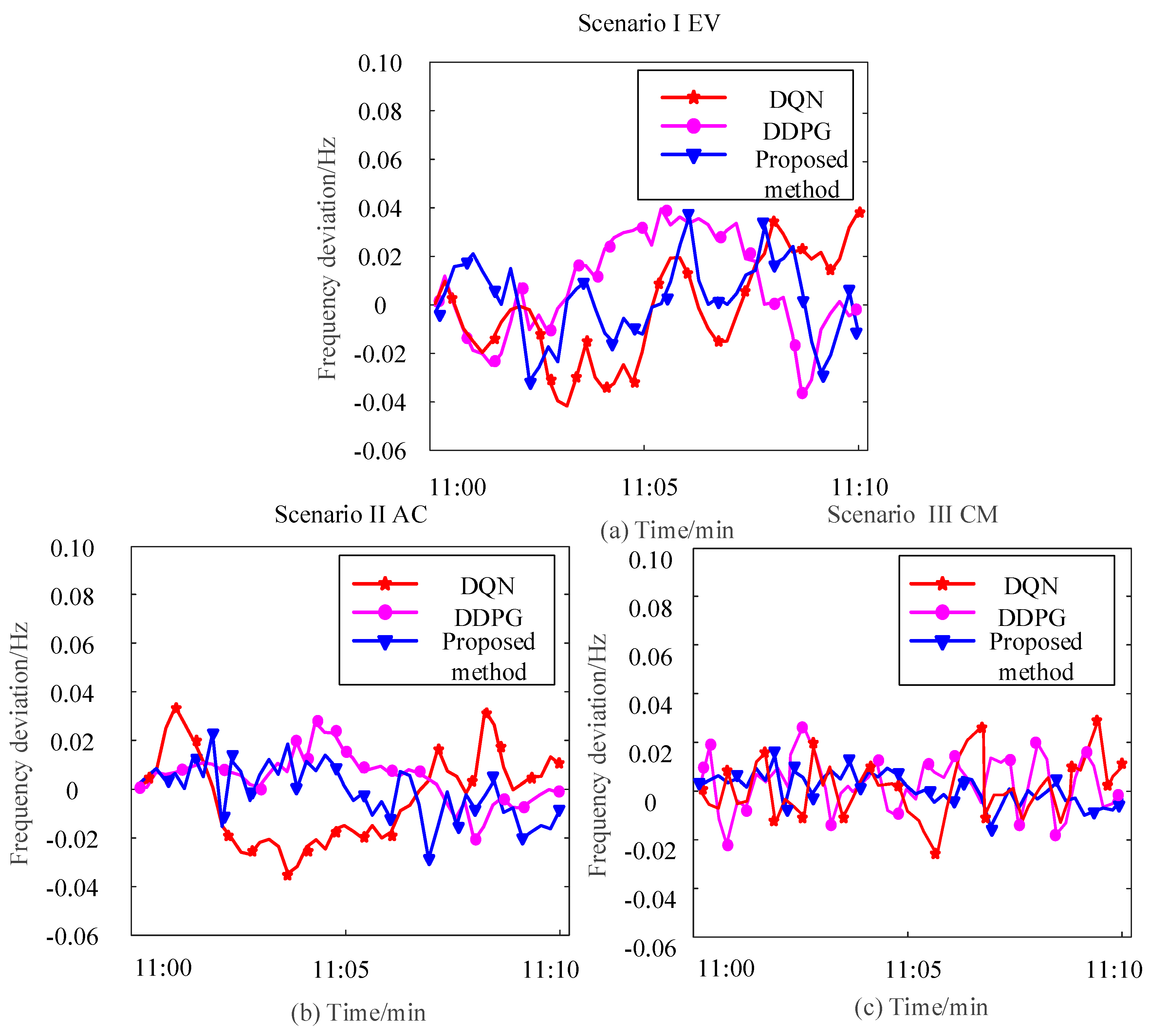
| Scenario I | (−0.039, 0.046) Hz | (−0.034, 0.042) Hz | (−0.030, 0.035) Hz |
| Scenario II | (−0.035, 0.041) Hz | (−0.030, 0.035) Hz | (−0.024, 0.026) Hz |
| Scenario III | (−0.028, 0.030) Hz | (−0.021, 0.027) Hz | (−0.017, 0.021) Hz |
| Performance Indicators | DQN | DDPG | Proposed Method |
|---|---|---|---|
| /Hz | 0.025 | 0.021 | 0.015 |
| t1/min | 14.9 | 21.6 | 5.1 |
| t2/s | 0.0056 | 0.0088 | 0.0043 |
| Performance Indicators | DQN | DDPG | Proposed Method |
|---|---|---|---|
| /Hz [37,38,39,40] | 0.105 | 0.034 | 0.020 |
| Max | 0.028 | 0.025 | 0.015 |
| t1/min | 15.2 | 24.4 | 6.3 |
| t2/s | 0.0113 | 0.0154 | 0.0096 |
| Weighting Factor | 1 | 0.8 | 0.6 | 0.4 | 0.2 |
| (Hz) | 0.012 | 0.014 | 0.016 | 0.019 | 0.021 |
| (yuan) | 5998 | 5904 | 5745 | 5803 | 5769 |
Disclaimer/Publisher’s Note: The statements, opinions and data contained in all publications are solely those of the individual author(s) and contributor(s) and not of MDPI and/or the editor(s). MDPI and/or the editor(s) disclaim responsibility for any injury to people or property resulting from any ideas, methods, instructions or products referred to in the content. |
© 2025 by the authors. Licensee MDPI, Basel, Switzerland. This article is an open access article distributed under the terms and conditions of the Creative Commons Attribution (CC BY) license (https://creativecommons.org/licenses/by/4.0/).
Share and Cite
Yu, G.; Li, X.; Chen, T.; Liu, J. Load Frequency Control via Multi-Agent Reinforcement Learning and Consistency Model for Diverse Demand-Side Flexible Resources. Processes 2025, 13, 1752. https://doi.org/10.3390/pr13061752
Yu G, Li X, Chen T, Liu J. Load Frequency Control via Multi-Agent Reinforcement Learning and Consistency Model for Diverse Demand-Side Flexible Resources. Processes. 2025; 13(6):1752. https://doi.org/10.3390/pr13061752
Chicago/Turabian StyleYu, Guangzheng, Xiangshuai Li, Tiantian Chen, and Jing Liu. 2025. "Load Frequency Control via Multi-Agent Reinforcement Learning and Consistency Model for Diverse Demand-Side Flexible Resources" Processes 13, no. 6: 1752. https://doi.org/10.3390/pr13061752
APA StyleYu, G., Li, X., Chen, T., & Liu, J. (2025). Load Frequency Control via Multi-Agent Reinforcement Learning and Consistency Model for Diverse Demand-Side Flexible Resources. Processes, 13(6), 1752. https://doi.org/10.3390/pr13061752