Deep Learning-Based Fluid Identification with Residual Vision Transformer Network (ResViTNet)

Abstract

The tight sandstone gas reservoirs in the LX area of the Ordos Basin are characterized by low porosity, poor permeability, and strong heterogeneity, which significantly complicate fluid type identification. Conventional methods based on petrophysical logging and core analysis have shown limited effectiveness in this region, often resulting in low accuracy of fluid identification. To improve the precision of fluid property identification in such complex tight gas reservoirs, this study proposes a hybrid deep learning model named ResViTNet, which integrates ResNet (residual neural network) with ViT (vision transformer). The proposed method transforms multi-dimensional logging data into thermal maps and utilizes a sliding window sampling strategy combined with data augmentation techniques to generate high-dimensional image inputs. This enables automatic classification of different reservoir fluid types, including water zones, gas zones, and gas–water coexisting zones. Application of the method to a logging dataset from 80 wells in the LX block demonstrates a fluid identification accuracy of 97.4%, outperforming conventional statistical methods and standalone machine learning algorithms. The ResViTNet model exhibits strong robustness and generalization capability, providing technical support for fluid identification and productivity evaluation in the exploration and development of tight gas reservoirs.

1. Introduction

Fluid identification is an indispensable aspect of reservoir evaluation, playing a pivotal role in the exploration and development of oil and gas fields. As noted by Fang et al. [1], accurate differentiation between fluid types such as gas, water, and their coexistence is crucial for formulating effective extraction strategies and improving reservoir management decisions. However, as exploration increasingly targets unconventional reservoirs, traditional fluid identification methods face significant challenges due to complex geological characteristics and reservoir heterogeneities, including low porosity, ultra-low permeability, and intricate fluid distributions. In China, where conventional oil and gas reserves are declining and development is entering a more mature phase, tight oil and gas—especially tight sandstone gas—have become critical resources for boosting reserves and production, as highlighted by Jia et al. [2].

Tight sandstone reservoirs, characterized by their low porosity, low permeability, and pronounced heterogeneity, present substantial difficulties for conventional petrophysical logging methods. Traditional approaches, including resistivity-based logging and empirical crossplot analyses, frequently encounter limitations in distinguishing between gas zones and water-bearing layers, especially under conditions of minimal differentiation in log responses [3]. For instance, techniques relying on rock physics models and simple geophysical logging parameters such as resistivity and porosity often prove inadequate when dealing with the complex geological conditions typical of tight gas formations [4,5]. Additionally, statistical methods employing historical production data or empirical models, though computationally efficient, are constrained by their reliance on linear assumptions and lower dimensional parameter interactions, as discussed by Tan et al. and Yan et al. [6,7]. Thus, there is a compelling need to develop advanced, robust methodologies capable of effectively addressing the nonlinear and high-dimensional characteristics intrinsic to tight gas reservoir evaluation.

In recent years, deep learning methods have emerged as powerful tools for fluid identification, particularly in tight reservoirs, due to their superior ability to automatically extract complex, high-dimensional features from extensive datasets. Studies such as those by He et al. and Li et al. [8,9] have demonstrated the success of convolutional neural networks (CNNs) in capturing subtle patterns within reservoir logging data. Moreover, integrating CNNs with architectures like long short-term memory (LSTM) networks significantly enhances the accuracy of fluid identification by simultaneously capturing spatial and temporal characteristics inherent in well log datasets. Despite these advances, standalone CNN models and other traditional machine learning methods often fail to fully exploit global context information and long-range dependencies present in the data, thereby limiting their performance and generalization capabilities [10,11].

Addressing these limitations, researchers including Zheng et al. [12] have proposed combining vision transformers (ViTs) with CNNs to leverage both local feature extraction and global context modeling. The hybrid ResViTNet model, which integrates ResNet and ViT architectures, represents a significant advancement by facilitating the efficient and accurate identification of complex fluid types through the transformation of logging data into multi-dimensional thermal maps. This approach enhances the discriminative power of logging parameters, such as resistivity (RT), neutron log (CNL), and bulk density (DEN), by visualizing their spatial variability clearly, thus improving classification accuracy.

In addition to earlier developments, recent studies from 2023 to 2025 have further advanced the application of deep learning in fluid identification. Qian et al. [13] incorporated prestack lithologic and petrophysical parameters into deep learning frameworks for tight sandstone prediction, while Gong and Zhang [14] developed a CNN–transformer hybrid model enhanced by wavelet transforms to improve classification performance in fractured reservoirs. These works demonstrate the increasing trend toward combining spatial, temporal, and frequency-domain representations in fluid property modeling, which directly inspires our ResViTNet design.

This study introduces the ResViTNet model to address fluid identification challenges specifically in the tight sandstone gas reservoirs of the Ordos Basin’s eastern Linxing area. By employing advanced data preprocessing techniques, including thermal map transformation and sliding window sampling strategies, this model efficiently manages data heterogeneity and class imbalance issues, providing a robust framework for fluid type classification. As shown in our prior work, comparative analyses demonstrate that ResViTNet significantly outperforms traditional triple-porosity methods, decision tree classifiers, and conventional CNN or ViT standalone models, achieving an accuracy of 97.4% and high consistency with expert manual interpretations.

Furthermore, the present work establishes a comprehensive, systematic technical framework, including a Python-based intelligent fluid identification system utilizing ResViTNet, capable of automated digital processing, model training, inference, and results visualization. The proposed method’s practicality is reinforced by extensive validation using real-world data from multiple wells, highlighting its strong stability, robustness, and potential for engineering deployment in complex geological scenarios.

In summary, traditional fluid identification methods largely depend on reservoir physical parameters such as porosity, permeability, and water saturation, while conventional machine learning models often struggle to capture global contextual information and long-range dependencies in logging data. This study introduces a deep learning-based approach aimed at improving fluid identification accuracy in tight sandstone reservoirs, thereby providing technical support for optimized reservoir management and enhanced recovery. Future research will further explore end-to-end modeling strategies based on raw logging data and integrate multi-source geophysical information to expand the applicability and generalization capability of the ResViTNet model in more complex reservoir settings.

2. Related Work

2.1. Traditional Fluid Identification Techniques

Traditional methods for fluid identification primarily rely on rock physics models and geophysical logging techniques. Lu Yuzhou et al. (2004) [15] effectively identified reservoir fluid properties by analyzing the response differences in parameters such as resistivity ratios, clay content, and porosity. Similarly, Tian Zhongyuan et al. (2005) [16] achieved promising results in identifying low-resistivity oil layers in the X oilfield by jointly analyzing resistivity and porosity parameters. However, in tight gas reservoirs characterized by low porosity and low permeability, traditional approaches often fail to capture effective information. The highly variable reservoir conditions further constrain the applicability of these methods.

Statistical methods, on the other hand, attempt to identify fluid types by analyzing historical production data and constructing empirical or probabilistic models. Sima Liqiang et al. (2005) [17] successfully discriminated fluid types in the Jia 2 Member reservoirs of southern central Sichuan using porosity-resistivity crossplots. Yuan Yu et al. (2013) [18] proposed a probabilistic crossplot-based approach, which improved identification accuracy by computing the probability distributions of different fluid types. Although statistical methods are computationally efficient and can provide rapid preliminary assessments in low-dimensional settings, they often rely on assumptions of linear relationships among variables. This limitation hampers their ability to capture nonlinear interactions among multiple parameters in complex reservoirs, thereby reducing their effectiveness in high-dimensional, strongly coupled scenarios.

Therefore, it is imperative to introduce deep learning methods capable of automatic feature extraction and high-dimensional modeling to enable more accurate fluid identification and comprehensive reservoir characterization.

2.2. Research Progress in Deep Learning-Based Fluid Identification

As a critical component of unconventional natural gas resources, tight gas reservoirs face substantial challenges in fluid identification due to complex geological conditions, diverse fluid types, and limited availability of effective data [19]. In recent years, significant progress has been made by researchers both domestically and internationally in addressing these issues. As a prominent branch of artificial intelligence, deep learning has demonstrated considerable potential for application in fluid identification and hydrocarbon exploration.

China is endowed with abundant tight gas resources, particularly in the Ordos and Sichuan basins, making them focal points of current research. However, existing machine learning methods still encounter limitations in feature extraction and in the modeling of complex data structures, which impedes their ability to meet the high precision and robustness requirements for fluid identification in tight gas reservoirs [20]. As a result, an increasing number of researchers have turned to deep learning techniques to address these challenges.

Compared with traditional machine learning, deep learning—particularly convolutional neural networks (CNNs)—offers enhanced capabilities for the autonomous extraction of high-dimensional features. CNNs are well-suited for learning and distinguishing subtle fluid-related patterns from log images, thus significantly improving classification accuracy. For instance, Luo Gang et al. [21] combined CNNs with long short-term memory (LSTM) networks to capture both spatial and temporal features of well log data, which substantially improved the accuracy of fluid identification in tight sandstone reservoirs. Qian Yugui et al. [13] integrated prestack lithologic and petrophysical sensitivity parameters as input features and employed prestack inversion alongside deep learning algorithms to quantitatively predict sandstone thickness and reservoir parameters.

Dongxiao Z [22] addressed missing data in logging sequences by applying recurrent neural networks (RNNs) for predictive data imputation, significantly enhancing data completeness. An Peng et al. [23] used LSTM networks to predict porosity and clay content, achieving a markedly lower error rate compared to traditional fully connected neural networks (FCNNs). Furthermore, Liu, W. et al. [24] incorporated contextual information into production forecasting by combining production trends with LSTM models, yielding favorable practical results.

In addition, Gong An and Zhang Heng [14] proposed a hybrid fluid identification model that integrates wavelet transform with a CNN-transformer architecture. Their approach effectively captures both frequency-domain and spatial features, achieving improved classification accuracy in fractured tight reservoirs. This further demonstrates the advantages of combining deep learning with advanced signal processing techniques.

These studies collectively demonstrate that deep learning methods outperform conventional machine learning approaches in capturing hidden nonlinear features within well log data and offer strong support for the accurate prediction of reservoir parameters.

3. Method

3.1. Well Log Data Collection and Preprocessing

The study was conducted in the Linxing (LX) block, located in the eastern margin of the Ordos Basin, one of China’s major regions for unconventional natural gas development. The area is typified by tight sandstone reservoirs exhibiting low porosity (5–12%) and low permeability (<0.1 mD), which pose significant challenges for fluid identification [2,25,26]. The Linxing block, in particular, has been identified as a promising exploration target due to its favorable gas generation potential and complex geological conditions. According to Zhu et al. [25], the Linxing–Shenfu gas field demonstrates a multi-layered accumulation pattern under the control of source–reservoir–fault systems, while Mi et al. [26] highlighted the presence of thick channel sand bodies with variable properties across microfacies. These geological characteristics underscore the necessity for advanced identification methods.

This study utilizes well log data collected from over 80 wells in the Linxing east block, a subregion known for its diverse geological settings and reservoir characteristics. All data were initially labeled by experienced technical personnel and subsequently validated by multiple domain experts [14], ensuring the reliability and scientific rigor of the dataset. This high-quality dataset provides a solid foundation for model development and evaluation.

Each input heatmap used by the model was generated from continuous logging curves spanning a 0.5 m-depth interval. Individual samples were interpreted by experts based on the dominant fluid type within that interval. To achieve well-level fluid classification during prediction, we employed a majority voting strategy to aggregate the predictions of all sampling segments from the same well interval, thus determining the primary fluid type for that section.

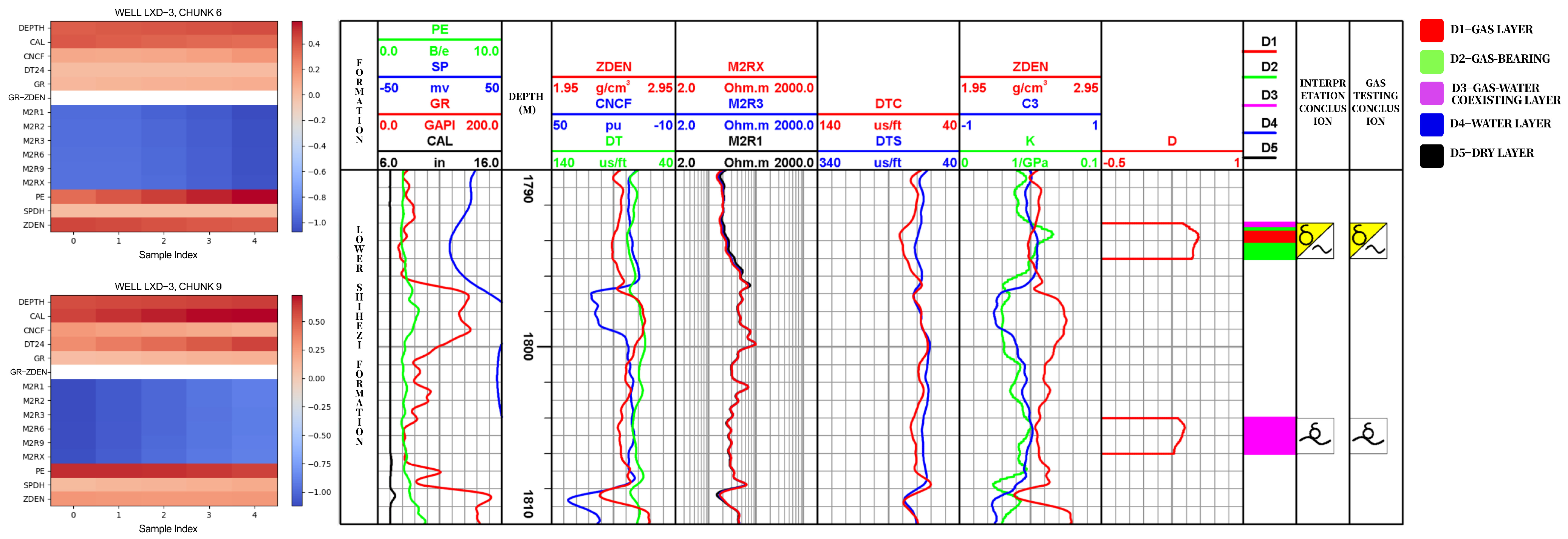
To further validate the interpretability and practical effectiveness of the proposed ResViTNet model, a representative well interval was selected for case analysis. In Figure 1, the left panel displays the thermal map generated by the model, where darker colors indicate higher predicted probabilities of gas zones. The right panel presents the conventional fluid interpretation results based on standard logging curves and geological knowledge, delineating gas zones, water-bearing gas zones, gas–water coexisting zones, and water zones. A strong consistency can be observed between the two methods across various depth intervals, especially in identifying thin interbedded layers and heterogeneous regions. This demonstrates that the ResViTNet model not only achieves high classification accuracy but also possesses strong adaptability to geological complexity, providing valuable support for the practical development of tight gas reservoirs.

To comprehensively characterize reservoir lithology, pore structure, and fluid properties, nine commonly used logging curves were selected as input features. These include acoustic time difference (AC), compensated neutron log (CNL), natural gamma ray (GR), spontaneous potential (SP), true resistivity (RT), bulk density (DEN), and caliper log (CAL), among others. These parameters collectively capture reservoir porosity, hydrogen content, lithological variation, permeability, and fluid characteristics, offering multidimensional and complementary information for the model. In particular, parameters such as RT, CNL, and DEN exhibit significant variations across different fluid types, thereby enhancing classification discriminability.

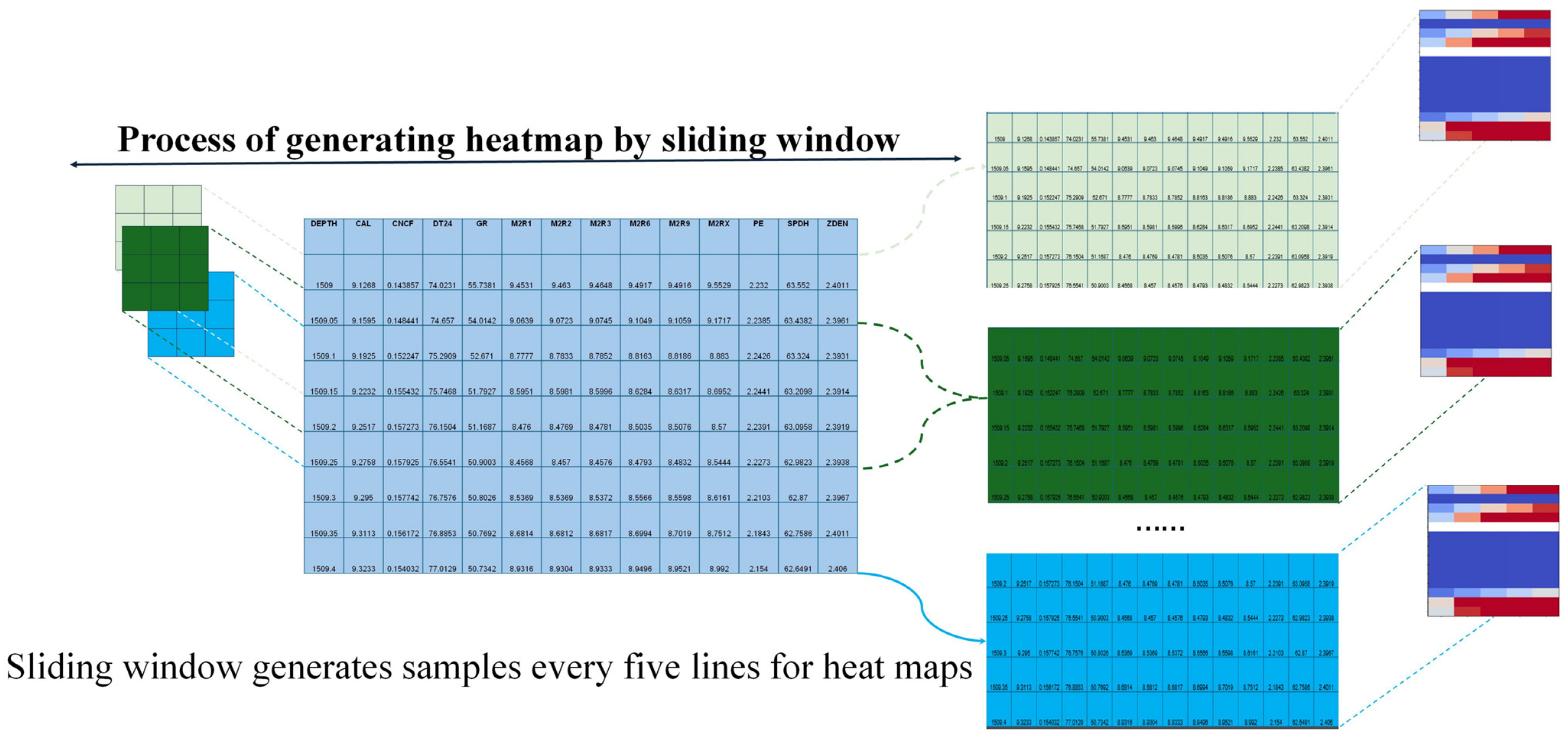
During data preprocessing, a sliding-window row-wise sampling strategy was employed, with a window length set to 0.5 m. Every five rows of logging data were transformed into a thermal map and labeled with the corresponding fluid type. This strategy increases data diversity and model coverage, ultimately generating 16,800 thermal map samples, comprising gas zones (5000), water zones (6000), water-bearing gas zones (3000), and gas–water coexisting zones (2800).

To address class imbalance, a hybrid sampling strategy combining oversampling of minority classes and undersampling of majority classes was adopted to balance the sample distribution and reduce model bias toward dominant categories. The optimized dataset was then split into training, testing, and validation sets in a ratio of 70%, 20%, and 10%, respectively, ensuring reasonable data distribution and fair model evaluation. Additionally, to enhance the model’s perception of spatial patterns in the logging data, multi-channel standardization was applied. Logging parameters were mapped onto RGB channels to generate uniformly formatted thermal maps, as illustrated in Figure 2. This representation preserves the coupling relationships among logging parameters while improving the separability of different reservoir types.

3.2. ResViTNet Model Architecture

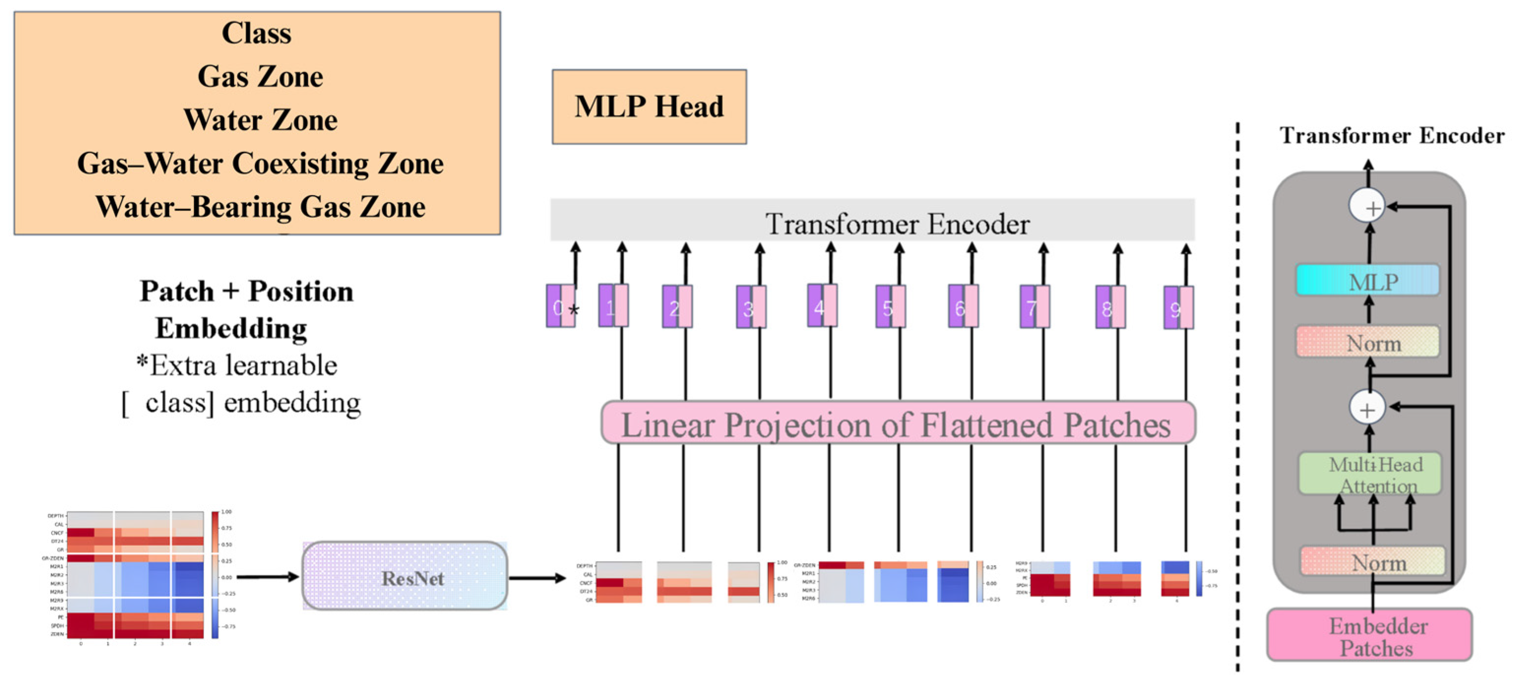
To enhance the accuracy and robustness of fluid identification in tight gas reservoirs, this study proposes a hybrid deep learning model—ResViTNet—that integrates convolutional neural networks (CNNs) with vision transformers (ViTs). The model leverages the local feature extraction capabilities of ResNet and the global context modeling strength of the transformer architecture, enabling efficient and automated fluid classification under complex reservoir conditions. As illustrated in Figure 3, the overall architecture comprises the following four main modules: input preprocessing, ResNet-based feature extraction, positional encoding with transformer encoders, and an output classification layer.

3.2.1. Well Log Input Normalization and Formatting

At the input stage, multi-channel thermal maps generated from well logging data are employed as the model input. All images are resized to a uniform resolution of 224 × 224 pixels to comply with the input specifications of the vision transformer (ViT). Through color mapping, the thermal maps vividly represent the spatial distribution of key logging parameters such as porosity, permeability, and resistivity. To improve training stability, all input images undergo normalization, with pixel values scaled to the [0, 1] range. This normalization mitigates scale discrepancies across various data sources, ensuring consistency and stability in model input.

3.2.2. Local Feature Extraction Module Based on ResNet

The input thermal maps are first passed through ResNet152 for feature extraction. The residual structure of ResNet effectively mitigates the vanishing gradient problem commonly encountered in deep neural networks, thereby enhancing the model’s ability to capture fine-grained details within complex reservoir images. The fundamental unit of ResNet is the residual block, which is mathematically expressed as follows:

$$y=F(x,\{Wi \})+x$$

(1)

where $y$ denotes the output of convolutional operations, $x$ is the input, and $\{Wi \}$ represents the set of convolutional weights. By introducing skip connections, the model preserves input information and enhances feature propagation across layers. After multiple convolution and pooling operations, ResNet produces feature maps enriched with local spatial information. These features are subsequently processed using global average pooling to reduce dimensionality, thereby improving computational efficiency.

3.2.3. Transformer-Based Global Encoding Module

At the core of the vision transformer (ViT) is the transformer encoder, which leverages a self-attention mechanism to effectively capture global dependencies within the image. The feature maps output by the ResNet module are first divided into multiple image patches of size 16 × 16 pixels. Each patch is then flattened and projected into a vector space via a linear transformation. This process can be formally expressed as follows:

$${z_0}^p =E(x_p)$$

(2)

where $x_p$ denotes the p-th image patch and represents the learnable linear projection matrix. Through this projection operation, each image patch is mapped into a fixed-dimensional embedding vector, which serves as the input to the transformer. To enable the model to capture the relative spatial positions among the patches, ViT incorporates positional encoding, which is shown in the following equation:

$$z_0 =[{z_0}^1+p_1 ,{z_0}^2 +p_2 ,\dots ,{z_0}^N +p_N]$$

(3)

where $p_i$ denotes the positional encoding which ensures that spatial information of the image patches is preserved within the self-attention mechanism. The core of self-attention lies in computing the pairwise dependencies among patches to capture global contextual features. The computation is formally defined as follows:

$$Attention(Q,K,V)=softmax(\frac{Q{K}^T}{\sqrt{d_k}}) V$$

(4)

where $Q$ denotes the query matrix, $K$ the key matrix, and $V$ the value matrix, all of which are obtained from the input embeddings via linear transformations. The term $d_k$ represents the dimensionality of the key vectors. Through this mechanism, the model is able to effectively capture long-range dependencies among image patches, enabling it to model global patterns and features within the image.

3.2.4. Output Layer and Classification

After processing by the transformer encoder, the resulting global embedding vector ${z_0}^L$ represents the holistic information of the input image. These global features are then passed through a classification head, which consists of a fully connected (linear) layer that maps the feature vector into the fluid-type category space. The probability distribution over the classes is computed using the following softmax function:

$$y=softmax(W{z_0}^L)$$

(5)

where $W$ denotes the weight matrix of the classification layer and the $softmax$ function is used to convert the output scores into probability values. Ultimately, the predicted fluid type corresponds to the class with the highest probability.

3.2.5. Loss Function

To optimize model performance, the cross-entropy loss function is employed to measure the discrepancy between the predicted results and the true labels. The loss is defined as follows:

$$L_{CE}(y,\widehat{y})=-{\displaystyle \sum _{i=1}^C{y}_i}log({\widehat{y}}_i)$$

(6)

where $C$ denotes the number of classes, $y_i$ represents the one-hot encoding of the true label, and $\widehat{y}$ is the predicted probability for class $i$. To address the issue of class imbalance, the following weighted cross-entropy loss function is adopted:

$$L_{WCE}(y,\widehat{y})=-{\displaystyle \sum _{i=1}^C{a}_i{y}_i}log({\widehat{y}}_i)$$

(7)

where $a_i$ represents the weight assigned to class $i$. A regularization term—such as L2 regularization—is also introduced to prevent model overfitting. The L2 regularization term is defined as follows:

$$L_{reg} ={\displaystyle \frac{\lambda }{2}}{\displaystyle \sum _{i=1}^n{W_i}^2}$$

(8)

where $W_i$ denotes the model weights and $\lambda$ is the regularization coefficient.

4. Experimental Results and Performance Evaluation

4.1. Experimental Dataset and Model Parameter Settings

To validate the effectiveness of the proposed ResViTNet-based reservoir fluid identification method, an experimental dataset was constructed using well logging data from 80 wells in the Linxing east block. The dataset encompasses the following five fluid types: gas zones, water-bearing gas zones, gas–water coexisting zones, water zones, and dry layers. After standardization, data augmentation was performed using a sliding window and row-wise sampling strategy, resulting in a total of 16,800 thermal map image samples. The dataset was split into 70% for training, 20% for validation, and 10% for testing.

Model training was carried out using the Adam optimizer with an initial learning rate of 0.0001, a batch size of 32, and a maximum of 200 training epochs. To mitigate overfitting, both L2 regularization and an early stopping mechanism were applied. Detailed hyperparameter configurations are provided in Appendix A.

4.2. Experimental Evaluation Metrics

In this study, several widely used multi-class evaluation metrics were adopted to comprehensively assess the classification performance of the ResViTNet model across different fluid types. These metrics include accuracy, confusion matrix, precision, recall, and F1-score. Multi-class classification tasks not only require the model to correctly distinguish between multiple categories but also necessitate a detailed evaluation of its performance on each individual class.

Among these metrics, the F1-score serves as a particularly important indicator for multi-class problems, especially in the context of imbalanced datasets. By incorporating both precision and recall, it provides a more balanced and holistic assessment of the model’s true classification capability. The confusion matrix provides an intuitive visual representation of the model’s predictions across categories, enabling a clear analysis of misclassification patterns. The specific formulas for these metrics are as follows:

$$\mathrm{Precision}={\displaystyle \frac{TP}{TP+FP}}$$

(9)

$$\mathrm{Recall}={\displaystyle \frac{TP}{TP+FN}}$$

(10)

$$F1=2\times {\displaystyle \frac{Precision\times Recall}{\mathrm{Re}call+Precision}}$$

(11)

where $TP$ (true positives) refers to the number of correctly identified samples, $FP$ (false positives) denotes the number of samples incorrectly predicted as the target class, and $FN$ (false negatives) represents the number of samples of the target fluid type that the model failed to identify.

4.3. Analysis of Experimental Results

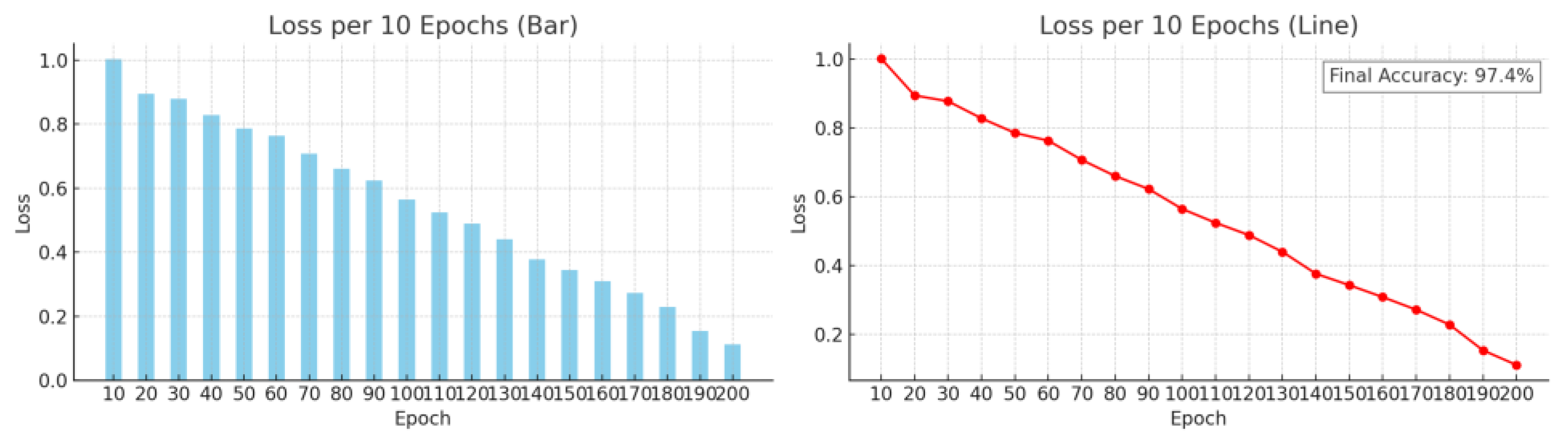
To provide a more intuitive understanding of the ResViTNet model’s training dynamics and performance, bar and line charts were employed to visualize the loss trends on both the training and validation sets across epochs, as shown in Figure 4. With the increase in training epochs, the training loss gradually decreases and the validation loss converges accordingly, demonstrating the effectiveness and robustness of the model.

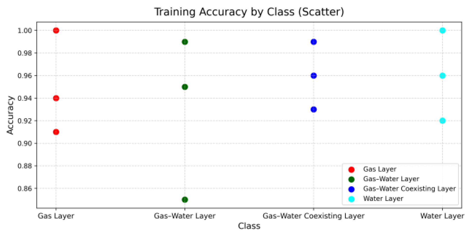
In addition, to evaluate classification performance at a more granular level, the PRF metrics—precision, recall, and F1-score—were adopted, and the F1-scores for each fluid category were presented using bar charts, as illustrated in Figure 5 and Figure 6. These visualizations provide a clear view of the model’s recognition performance across different fluid types [20]. Notably, the model achieves high F1-scores in identifying gas and water zones, whereas more complex categories—such as gas–water coexisting zones—still exhibit some prediction errors.

As evidenced by the aforementioned results, the bar charts clearly reveal the differences in classification accuracy across fluid types, indicating that the model performs well in most categories. However, for more challenging classes—such as gas–water coexisting zones—there is a need to further optimize both data quality and model architecture.

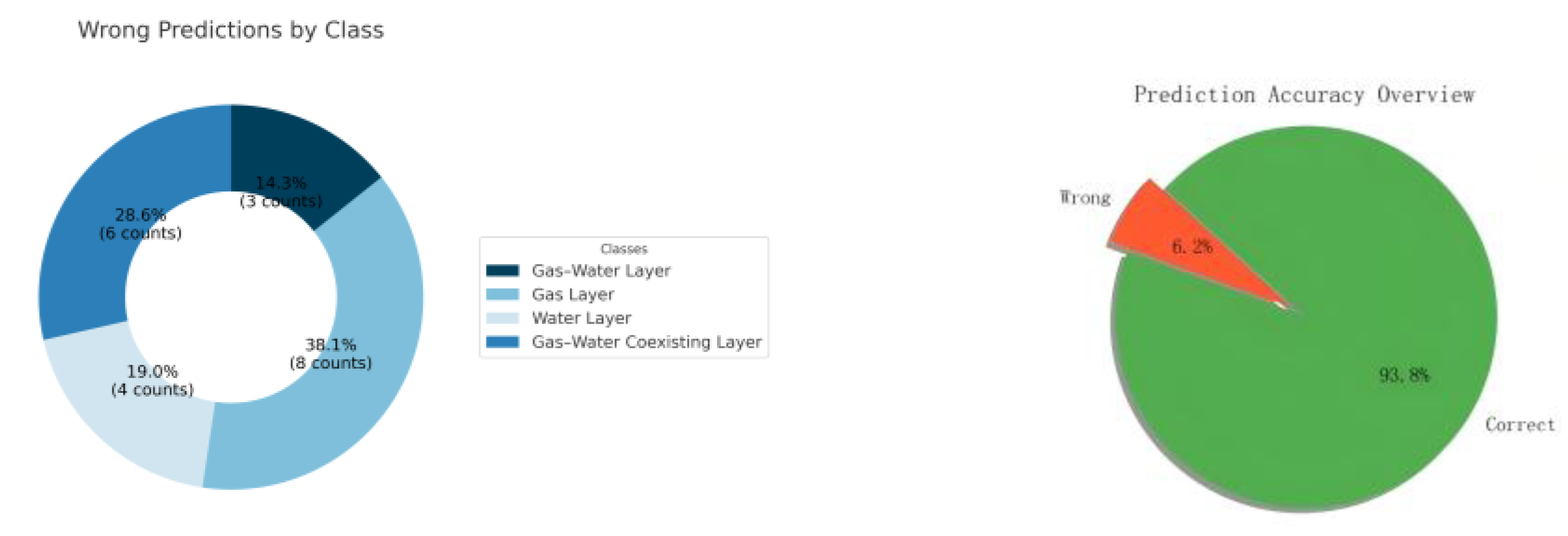
Further analysis (Figure 7) presents that although prediction errors still exist in some categories, the model demonstrates relatively high accuracy in identifying water zones and water-bearing gas zones, further confirming the robustness of ResViTNet in recognizing water-associated fluid layers. To comprehensively evaluate the misclassification behavior, a statistical analysis of the number and proportion of misclassified samples was conducted (Figure 8). The findings indicate that the overall misclassification rate is only 6.2%, with the majority of errors concentrated in the gas–water coexisting class. These results provide a clear insight for future algorithm refinement and data augmentation strategies.

A comparison of Figure 9 and Figure 10 provides an intuitive visual distinction between misclassified and correctly classified thermal maps. Misclassified thermal maps often exhibit relatively uniform white regions, with minimal visible color variation. Upon further analysis of the corresponding raw Excel data, it was found that the underlying values in these samples exhibited very limited variability, some even remaining nearly constant throughout.

This outcome is closely related to the normalization process, which rescales all data values between 0 and 1. When the original values already fall within a narrow range, normalization further compresses the differences, leading to an almost uniform distribution. Consequently, during the color encoding stage such subtle variations result in heatmaps that lack sufficient contrast or visible structure. These flat visual patterns make it more difficult for the model to extract useful features. The absence of meaningful variation in the input can significantly weaken the model’s ability to make accurate predictions. In practice, the model tends to rely on patterns, gradients, and contrasts within the thermal maps. When those cues are absent or too subtle to detect, the classification output becomes less reliable.

This observation highlights a potential vulnerability in the current system. When input data lacks variability, the visual representation fails to provide enough discriminative information for robust classification. Addressing this issue may involve refining the preprocessing strategy, such as enhancing contrast in low-variance samples or introducing additional domain-specific features to compensate for the lack of dynamic range.

4.4. Analysis of Ablation Experiments

To better understand the contribution of each component to the overall performance of the ResViTNet model, ablation experiments were conducted. By selectively removing specific modules from the model, we analyzed their impact on performance. The results are summarized in

Table 1. Ablation study of the ResViTNet model.

Model Variant	ResNet	Vision Transformer	Accuracy
ResViTNet	✓	✓	97.4
ResNet Only	✓	✗	93.1
ViT Only	✗	✓	94.0
Without Thermal Map	✓	✓	90.5
Without ResNet (ViT Only)	✗	✓	89.7

Note: ✓ indicates the presence of the module; ✗ indicates the absence of the module.

.

The complete ResViTNet model, which integrates both ResNet and ViT architectures with thermal map inputs, achieves the highest classification accuracy of 97.4%, demonstrating its superior performance. When the ViT module is removed and only the ResNet backbone is retained the accuracy drops to 93.1%, highlighting its strength in capturing local details but its relative weakness in global feature representation. Conversely, using ViT alone yields an accuracy of 94.0%, highlighting its strength in global feature representation but its relative weakness in capturing local details.

When the thermal map generation module is excluded, the accuracy further decreases to 90.5%, confirming the importance of thermal maps in enhancing the model’s understanding of complex geological data. Finally, when both ResNet and the thermal map module are removed, the model performs the worst, with an accuracy of only 89.7%, further underscoring the critical contributions of both components to overall model performance.

4.5. Model Comparison Experiments

To further evaluate the performance of ResViTNet in fluid identification, we conducted comparative experiments against other commonly used classification models, including ResNet and vision transformer. The results of this comparison are presented in

Table 2. Comparison of different models for fluid identification.

Model Name	Accuracy	Number of Parameters	Inference Time (s/Batch)
ResViTNet	97.4	45	0.85
ResNet152	93.1	60	0.70
VIT	94.0	100	1.20
ResNet101	88.5	30	0.65
ResNet50	85.7	25	0.60

Note: Bold values indicate the best performance in each metric.

.

The results of the comparative experiments demonstrate that the ResViTNet model outperforms its counterparts in terms of classification accuracy, parameter efficiency, and computational performance, achieving the best overall performance. The ResNet series models, while effective in extracting local features, exhibit relatively lower classification accuracy due to their limited capacity for modeling global dependencies. Although the vision transformer achieves relatively high accuracy, its computational efficiency is significantly reduced due to its large number of parameters.

Traditional convolutional models, such as ResNet50 and ResNet101, perform poorly in the complex fluid identification task, indicating limitations in their representational capacity and generalization ability. A comprehensive comparison between ResViTNet and traditional methods, standalone CNNs, and other mainstream deep learning models is presented in

Table 3. Comparison with traditional fluid identification methods.

Method	Accuracy (%)	F1-Score (%)
Triple-Porosity Overlap Method	83.5	0.820
Decision Tree Classification Method	88.1	0.874
ResNet152	93.2	0.928
ViT	91.7	0.911
ResViTNet	97.4	0.968

Note: Bold values indicate the best performance in each metric.

. The comparison includes the conventional triple-porosity overlap method, decision tree classifier, ResNet152, and the base vision transformer model.

The comparative analysis indicates that the ResViTNet model significantly outperforms other methods in both accuracy and F1-score. In particular, it provides more stable and reliable classification results under complex geological conditions, demonstrating strong practical applicability and engineering deployment potential.

4.6. Analysis of Classification Metrics

To comprehensively evaluate the classification performance of the model, we analyzed its performance using F1-score, precision, and recall metrics. The results of the F1-scores and PRF (precision, recall, F1-score) metrics for each fluid category are summarized in

Table 4. Classification metrics of different models.

Class	Accuracy	Precision	Recall	F1-Score
Water Zone	97.0	96.8	97.2	0.970
Gas Zone	97.5	97.1	97.9	0.975
Gas–Water Coexisting Zone	93.5	93.1	94.0	0.935
Water-Bearing Gas Zone	96.2	95.8	96.5	0.962

.

The results indicate that the model performs particularly well in identifying gas zones and water zones, with F1-scores reaching 97.5% and 97.0%, respectively. Although the prediction accuracy for gas–water coexisting zones is comparatively lower, the model still demonstrates strong classification capabilities across all fluid categories. These findings further validate the robustness of the ResViTNet model in the challenging task of fluid identification in complex tight gas reservoirs.

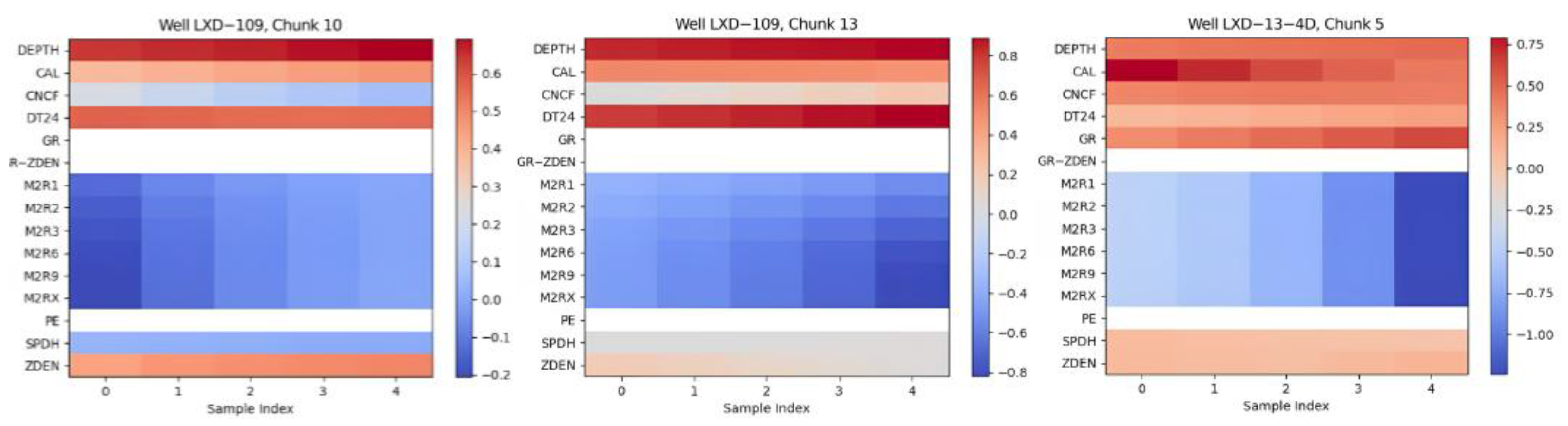
4.7. Interpretability and Causal Validation

In this study, based on the ResViTNet model, well logging curves were converted into thermal maps and segmented using a sliding window technique, resulting in a high-density sample set from continuous logging data. Each sample was independently input into the model for fluid type prediction. The primary fluid type for an entire well section was then determined by aggregating the prediction probabilities of all samples from that well [27]. The classification criterion was defined as follows: if the prediction error rate of individual samples within a well is below 5% and the majority of predictions are consistent, the fluid type for that well section is assigned accordingly.

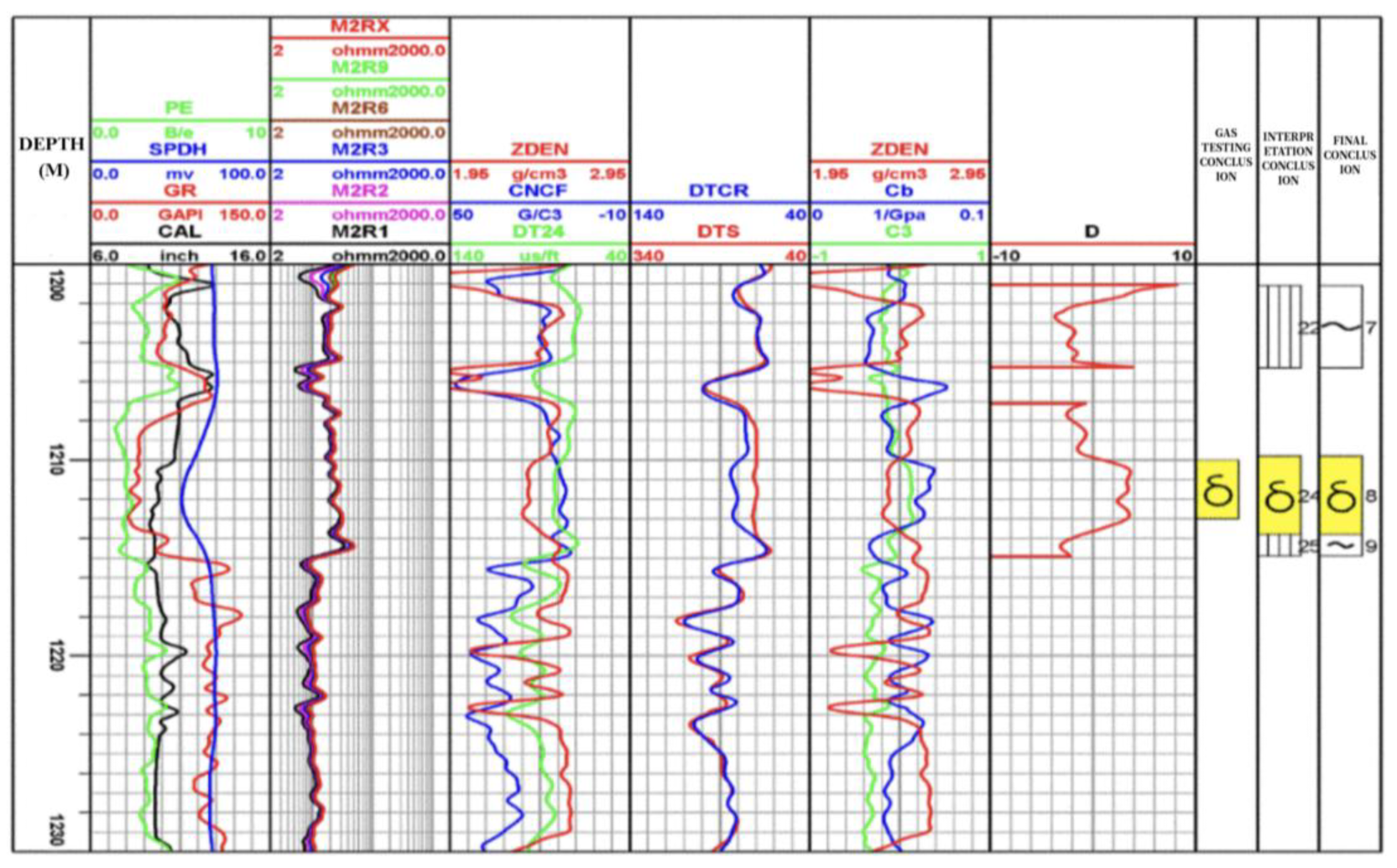
Taking Well LX-8 in the study area as an example, the ResViTNet model predicted that 97% of the samples corresponded to a gas zone, resulting in a comprehensive classification of this well section as a gas-bearing interval—an outcome highly consistent with manual interpretation. Figure 11 illustrates the fluid prediction results for Well LX-8. In the figure, the yellow segments indicate gas zones as predicted by the model, demonstrating that ResViTNet maintains high precision and well-defined classification boundaries even under complex geological conditions such as gas–water coexisting layers and interbedded thin layers. This validates the model’s adaptability to complex environments and its fine-grained recognition capability. Furthermore, experimental results show that the RT parameter presents a clear contrast between gas and water zones in the thermal maps, while the hydrogen content captured by the CNL displays distinct gradients, thereby significantly enhancing the model’s feature extraction and fluid classification accuracy [28].

4.8. Field Application Results

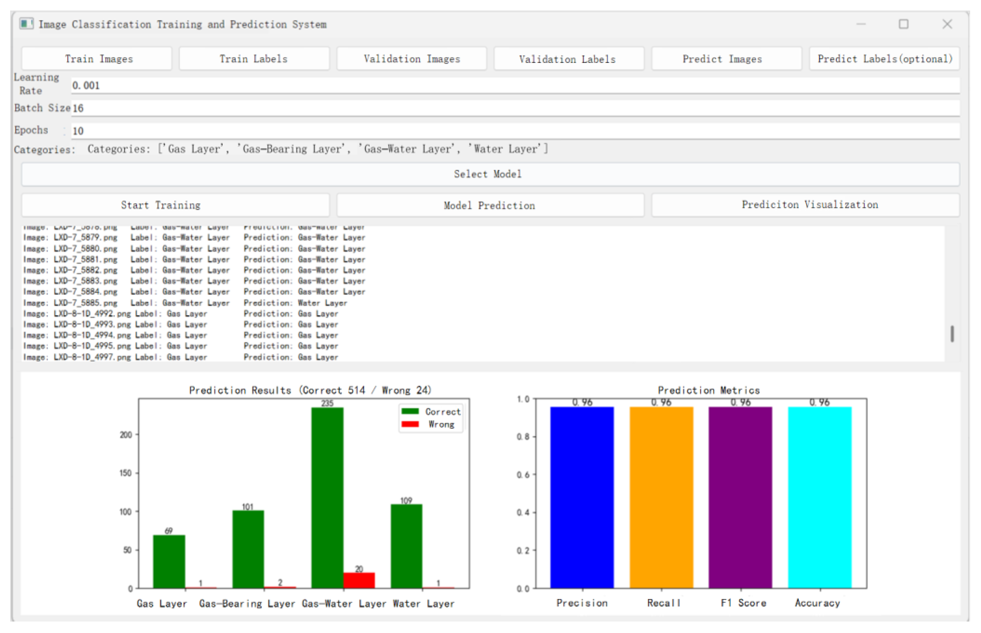
Based on the ResViTNet model, this study designed and developed an intelligent fluid identification and prediction system for tight gas reservoirs. The system was implemented using Python (v3.9) and PyQt5 (v5.15.7) and integrates functionalities such as digital processing of well logging data, model training and inference, and results visualization. It supports automated identification and prediction of fluid types.

Utilizing a sliding window strategy and thermal map transformation, the system generates high-density samples which are then processed by the pre-trained ResViTNet model to efficiently classify complex fluid types including gas zones, water zones, gas–water coexisting zones, and water-bearing gas zones. Additionally, the system supports model fine-tuning and retraining to adapt to varying geological conditions across different blocks.

The system provides comprehensive model performance evaluation and visualization tools, displaying key metrics such as classification accuracy, precision, recall, and F1-score. Moreover, it facilitates comparative analysis between model predictions and manual interpretations through visual comparisons of well profiles [29]. Field applications using real logging data from multiple tight gas reservoir blocks have demonstrated the system’s strong stability and generalization capabilities in complex fluid identification tasks [30]. The predicted results exhibit high consistency with expert interpretations, highlighting the system’s significant potential for engineering deployment (Figure 12).

5. Conclusions

In response to the challenges of fluid identification in tight gas reservoirs in the Linxing east area of the Ordos Basin—specifically the low accuracy of traditional methods under complex geological conditions—this study proposes a deep learning model, ResViTNet, which integrates ResNet and vision transformer (ViT) architectures. By introducing a multi-channel thermal map representation of logging parameters and a sliding window sampling strategy, the model effectively combines local feature extraction with global dependency modeling, enabling efficient identification of various fluid types in tight gas reservoirs. The main conclusions of this study are as follows:

(1)

A reservoir fluid identification model based on ResViTNet was constructed, effectively combining the local feature extraction capability of ResNet and the global modeling strength of the transformer. The model achieved a classification accuracy of 97.4%, outperforming traditional triple-porosity crossplot methods, decision tree classifiers, and standalone CNN models.

(2)

Multiple experiments demonstrated that the use of thermal map representation and sliding window sampling significantly enhanced the expressiveness of the logging data, improving input diversity and feature discriminability. Ablation studies further confirmed the crucial role of the transformer encoder in enhancing global feature learning and improving the robustness of fluid identification.

(3)

The ResViTNet model exhibited excellent generalization ability and stability when dealing with high-dimensional, nonlinear, and multi-scale features. It effectively addressed the heterogeneity and complexity inherent in tight gas reservoirs, demonstrating strong potential for practical applications.

(4)

Despite achieving promising identification results, the current approach still has some limitations. The model primarily relies on thermal map-based data representation. Future work may explore end-to-end modeling methods based directly on raw logging curves to further enhance generalization and operational efficiency.

In summary, the ResViTNet model provides an efficient and accurate technical solution for fluid type identification in complex tight gas reservoirs. It holds significant promise for improving the scientific rigor of exploration and development decision-making. Future research will focus on optimizing the model architecture and incorporating multi-source geophysical data for integrated identification, thereby expanding its applicability to other types of complex hydrocarbon reservoirs. In addition, future efforts may explore the use of lightweight network structures to enhance deployment efficiency in edge computing scenarios. Incorporating uncertainty quantification into the model could also help improve interpretability and support risk-informed decision-making. These directions will further strengthen the model’s robustness and practical value across a broader range of subsurface conditions.