Leak Identification and Positioning Strategies for Downhole Tubing in Gas Wells

Abstract

Accurate detection of downhole tubing leakage in gas wells is essential for planning effective repair operations and mitigating safety risks in annulus pressure buildup wells. Current localization methods employ autocorrelation analysis to exploit the time-delay features of acoustic signals traveling through the tubing–casing annulus. This allows non-invasive wellhead detection, avoiding costly tubing retrieval or production shutdowns. However, field data show that multiphase flow noise, overlapping reflected waves, and coupled multi-leakage points in the wellbore frequently introduce multi-peak interference in acoustic autocorrelation curves. Such interference severely compromises the accuracy of time parameter extraction. To resolve this issue, our study experimentally analyzes how leakage pressure differential, aperture size, depth, and multiplicity affect the autocorrelation coefficients of acoustic signals generated by leaks. It compares the effects of different noise reduction parameters on leakage localization accuracy and proposes a characteristic time selection principle for autocorrelation curves, providing a new solution for precise leakage localization under complex downhole conditions.

1. Introduction

According to statistics from the International Energy Agency (IEA), global natural gas consumption resumed structural growth in 2024, reaching a historic high. Natural gas demand is projected to further increase in 2025, primarily driven by rapidly growing Asian markets [1]. However, as critical conduits for natural gas production, downhole tubing in gas wells—subjected to prolonged exposure to high temperatures, high pressures, hydrogen sulfide corrosion, and other complex operating conditions—are prone to leakage incidents. Such leaks not only result in resource waste and greenhouse gas emissions, but may also trigger well control risks [2,3,4,5,6,7].

In the field of leakage detection technology, existing methods can be categorized into direct detection and indirect inference approaches. Direct detection methods, represented by distributed fiber optic sensing (DTS/DAS), achieve real-time monitoring of temperature/strain variations through downhole fiber optic deployment, with localization accuracy reaching ±1 m [8,9,10]. However, this technology necessitates the pre-installation of specialized equipment, with single-well modification costs surpassing 800,000 yuan. Additionally, it cannot effectively detect sudden leaks in active production wells. Indirect inference methods primarily rely on acoustic wave analysis, among which autocorrelation function-based localization technology has attracted significant attention due to its advantage of not requiring downhole tool intervention. This technique locates leaks by analyzing the time difference of leak-induced acoustic wave propagation in the tubing–casing annulus.

Nevertheless, field applications reveal significant challenges for current acoustic localization technologies: On one hand, broadband noise generated by multiphase flow in the wellbore extensively overlaps with leakage signal frequency bands. On the other hand, the superposition effects of multiple reflected waves and multi-leak signals create false peaks in autocorrelation curves. Additionally, distinct acoustic waveforms generated by different leakage modes (such as pitting corrosion leaks and threaded connection leaks) further increase the uncertainty in characteristic time extraction. These technical bottlenecks severely limit the engineering applicability of acoustic localization methods under complex downhole conditions. To address these issues, this paper proposes a characteristic time selection principle for autocorrelation coefficient curves through statistical analysis of experimental data, providing a new solution for tubing leak localization based on acoustic signal autocorrelation. The experimental platform and methodology used in this study are detailed in reference [11].

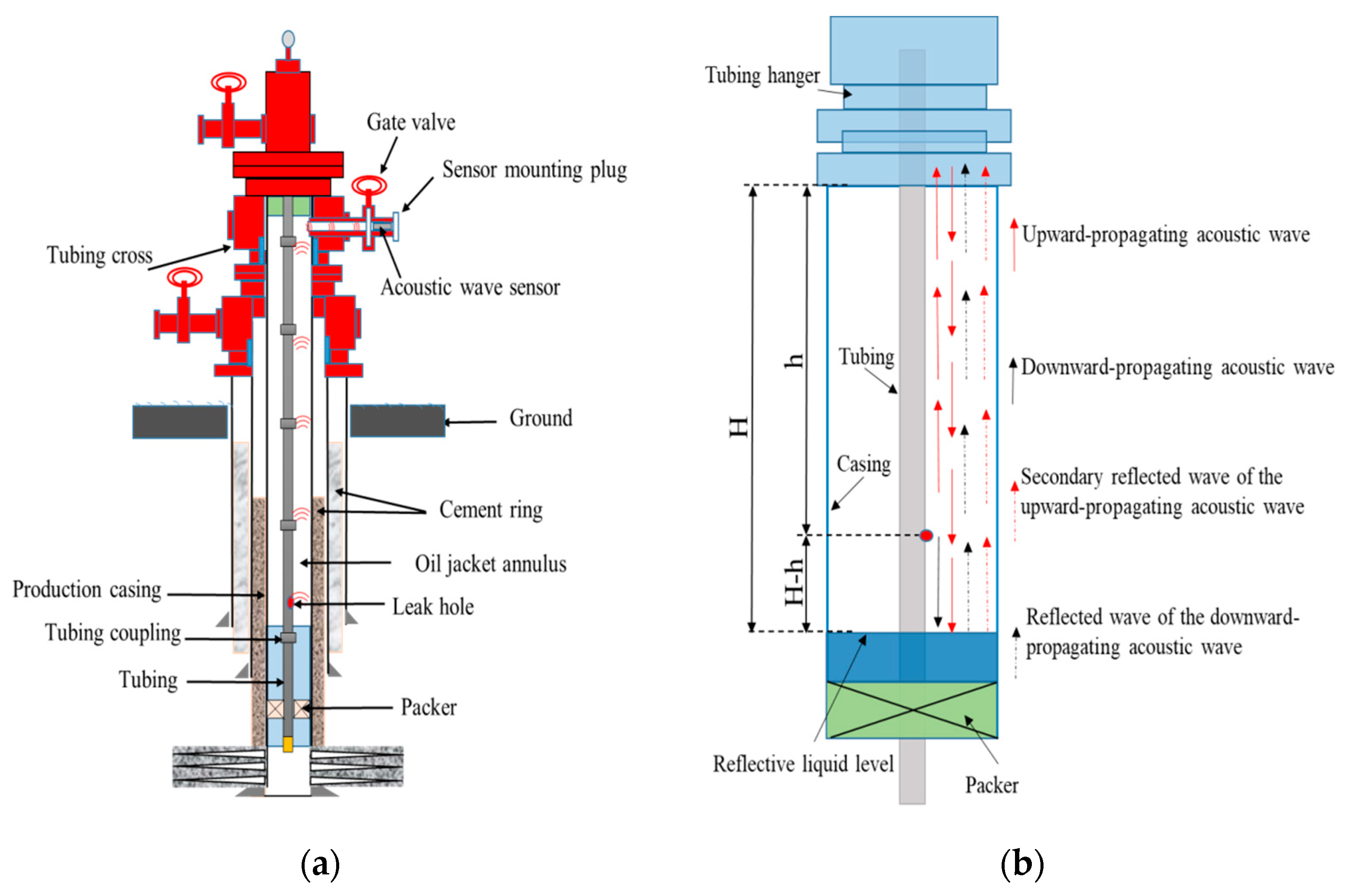
2. Principle of Tubing Leak Localization

Figure 1a shows a schematic diagram of downhole tubing leak detection in natural gas wells. The enclosed space formed by the tubing hanger, production casing, and annular protection fluid is referred to as the annulus. An acoustic sensor is installed at the annulus outlet to capture annular acoustic signals. By analyzing the time–frequency characteristics of the annular acoustic signals, the leakage status of downhole tubing can be identified and located.

Figure 1b illustrates the simplified propagation path of tubing leak acoustic waves. When a tubing leak occurs, acoustic waves propagate simultaneously upward and downward through the annulus. The upward-propagating waves travel directly toward the wellhead, while the downward-propagating waves reflect at the interface between the tubing hanger and annular protection fluid before returning to the wellhead. The time delay between the direct and reflected waves is correlated with the distance from the leak point to the annular protection fluid.

Let H denote the total annulus depth and h represent the distance from the leak point to the tubing hanger. The relationship between these parameters can be expressed as [11]:

$$\left\{\begin{array}{l}\overline{v}{t}_1=2\left(H-h\right)\\ \overline{v}{t}_2=2H\end{array}\right.,$$

(1)

Therefore, the leak depth (h) in the tubing can be calculated as:

$$h=\overline{v}\left(t_2-t_1\right)/2,$$

(2)

where $\overline{v}$ is the average propagation velocity of acoustic waves in the annular medium (m/s); t₁ represents the time delay between the upward-propagating leak acoustic wave and the downward-propagating/reflected wave arriving at the wellhead, corresponding to twice the distance between the leak point and annular protection fluid; and t₂ denotes the propagation time delay of reflected leak acoustic waves in the annulus, corresponding to twice the total annulus depth. As shown in Equation (2), the key to determining downhole tubing leak location lies in obtaining both the acoustic wave propagation velocity in the annulus and the characteristic times t₁ and t₂.

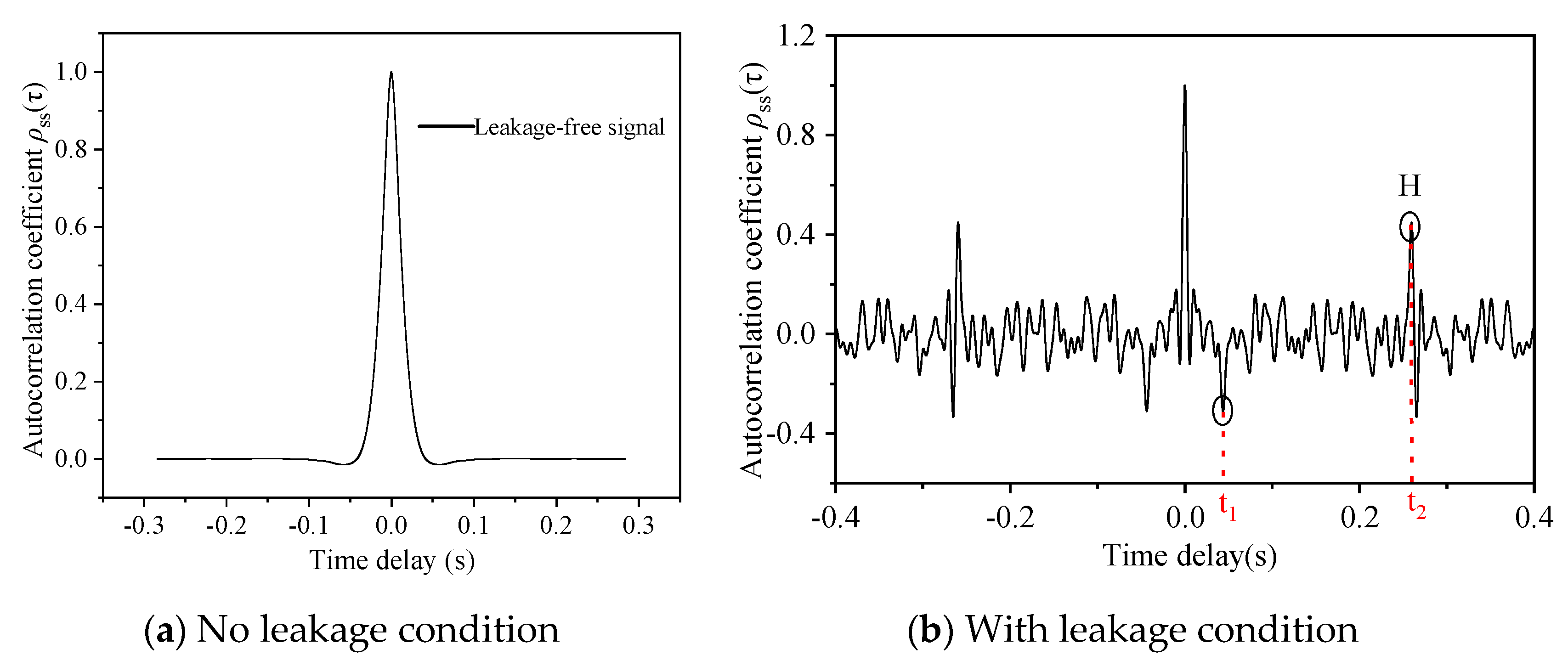
2.1. Extraction of Characteristic Time

Leakage acoustic signals often contain significant noise, which can be categorized into random noise and coherent noise.

• Random noise primarily originates from production noise, system noise, and field noise. Field noise, in particular, includes sounds generated during production operations, maintenance activities, and seawater impact on surface casing;
• Coherent noise mainly results from reflections of leakage-induced acoustic waves by downhole tubing collars, gas lift valves, or subsurface safety valves.

Random noise lacks autocorrelation properties and can be effectively filtered out through autocorrelation processing of the signal, thereby achieving noise reduction [12]. This is illustrated in Figure 2a.

In contrast, coherent noise shares the same physical nature as leakage acoustic waves and generates a series of interference peaks in the autocorrelation curve. However, since the reflection surfaces of annular obstructions (e.g., collars and valves) are significantly smaller than those of the tubing hanger and annular protection fluid, the resulting interference peaks exhibit lower amplitudes compared with the characteristic peaks used for leakage localization and fluid-level depth estimation.

Therefore, selecting an appropriate threshold for autocorrelation coefficient peaks is critical for improving the accuracy of leak point localization.

The autocorrelation function characterizes the correlation between two values of a random signal separated by a time interval $\tau$, and is defined as [13]:

$$R_{ss}\left(\tau \right)=E\left[s\left(t\right)s\left(t+\tau \right)\right],$$

(3)

In the equation, E[] represents the expectation operator and $\tau$ denotes the time delay.

In practical applications, $R_{ss}\left(\tau \right)$ can only be estimated. The estimation method is given by [14]:

$$R_{ss}\left(\tau \right)={\displaystyle \frac{1}{Tim}}{\displaystyle {\int }_0^{Tim-\tau }s\left(t\right)s\left(t+\tau \right)}dt,$$

(4)

In the equation, Tim represents the time window.

Typically, the autocorrelation function is expressed in normalized form, defined as:

$${\rho }_{ss}\left(\tau \right)={\displaystyle \frac{R_{ss}\left(\tau \right)}{\left|R_{ss}\left(0\right)\right|}},$$

(5)

This indicates that, when s(t) is correlated with s(t+$\tau$), ${\rho }_{ss}\left(\tau \right)$ will reach a peak value, manifesting as a distinct characteristic peak on the autocorrelation curve.

Theoretically, leakage acoustic signals generated at different locations or different times exhibit weak correlation, whereas signals originating from the same location and time demonstrate strong correlation. Consequently, performing autocorrelation analysis on the annular leakage acoustic signals yields the following set of characteristic times:

$$\tau \in \left\{0,\pm t_1,\pm \left(t_2-t_1\right),\pm n{t}_2,\pm \left(t_2+t_1\right),\cdots \right\},$$

(6)

As illustrated in Figure 1, the acoustic wave signal generated by tubing leakage propagates simultaneously toward both the wellhead and the bottom of the well. According to the localization principle:

(1) When $\tau$= t₁ = 2(H−h)/$\overline{v}$, ${\rho }_{ss}\left(\tau \right)$ reaches a negative extremum. This corresponds to:

• The characteristic time for leak point location;
• The abscissa (time coordinate) of the negative characteristic peak on the leakage acoustic wave’s autocorrelation curve.

(2) When $\tau$= t₂ = 2H/$\overline{v}$, ${\rho }_{ss}\left(\tau \right)$ reaches a positive extremum. This represents:

• The characteristic time corresponding to fluid level depth;
• The abscissa of the positive characteristic peak on the autocorrelation curve.

(3) Similarly, when $\tau$= 2nH/$\overline{v}$(n = 2, 3, 4,…), ${\rho }_{ss}\left(\tau \right)$ also attains positive extrema. These result from:

• Multiple reflections of the leakage acoustic wave within the annulus;
• Higher-order harmonic components in the signal.

The leakage location and annulus depth can be determined by extracting the abscissa values corresponding to the extrema of ${\rho }_{ss}\left(\tau \right)$, yielding characteristic times t₁ and t₂ from the autocorrelation curve. As shown in Figure 2b, this displays the autocorrelation coefficient curve of acoustic signals collected at the Christmas tree annulus outlet when only one leakage point exists in the tubing.

Since the autocorrelation function is even, the resulting curve exhibits symmetry about the zero point. This means that the characteristic peaks on the curve correspond to both positive and negative time delays, where the sign only indicates a temporal sequence without affecting the absolute magnitude of delay between acoustic signals. Therefore, this study focuses exclusively on the positive semi-axis.

Specifically:

• t₁ corresponds to the abscissa of the first maximum negative characteristic peak on the autocorrelation curve;
• t₂ represents the abscissa of the first maximum positive characteristic peak;
• The series of minor characteristic peaks result from reflections of leakage acoustic waves by downhole tubing collars, gas lift valves, or subsurface safety valves.

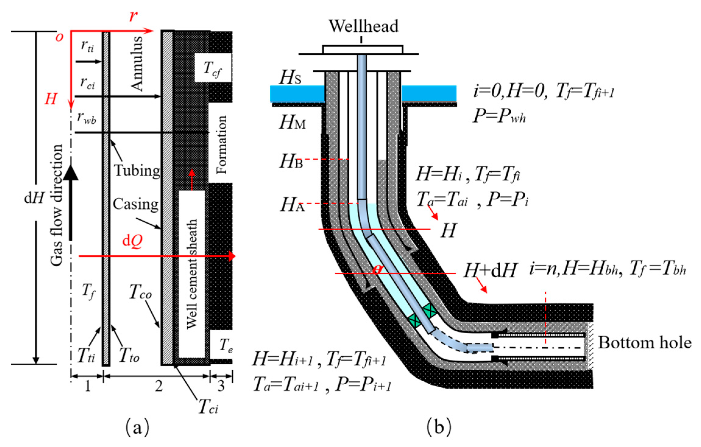
2.2. Determination of Annular Acoustic Velocity

The American Gas Association (AGA) Report 10 provides the calculation formula for natural gas acoustic velocity, which is primarily influenced by gas composition, temperature, and pressure [15]:

$$c={\left[\left(kRT/M_g\right)\left(Z_g+\rho {\left({\displaystyle \frac{\partial Z_g}{\partial \rho }}\right)}_{T_g}\right)\right]}^{1/2},$$

(7)

where k is the specific heat ratio (dimensionless); R denotes the molar gas constant (J/mol·K); T represents the gas temperature (K); M is the molar mass of natural gas (kg/mol); Z_g stands for the natural gas compressibility factor (dimensionless); and $\rho$ indicates the gas molar density (mol/m³).

The molar density and compressibility factor are calculated using the empirical equations proposed by Cockrell, employing the PR (Peng–Robinson) equation of state [16]. Prior to determining the annular acoustic velocity, it is necessary to establish the annular temperature and pressure distributions. In production wells, heat transfer occurs between the produced gas and surrounding media due to temperature differentials. The temperature profile along the wellbore can be derived based on energy balance and heat transfer equations, under the following assumptions:

• Steady-state conditions prevail for heat transfer within the wellbore, while transient heat transfer dominates between the wellbore and formation;
• Only radial heat transfer is considered;
• Formation temperature exhibits a linear variation with depth [17,18].

Consequently, the equilibrium equation for a differential element dH, as illustrated in Figure 3 [19], can be expressed as:

$${\displaystyle \frac{d{T}_f}{dH}}={\displaystyle \frac{1}{C_{pm}}}\left({\displaystyle \frac{dQ}{w_{t}dH}}-g\sin \theta -{\displaystyle \frac{udu}{dH}}\right)+C_J{\displaystyle \frac{d{p}_f}{dH}},$$

(8)

where T_f is the temperature of natural gas in the tubing (K); H denotes the measured well depth (m); C_pm represents the constant-pressure specific heat capacity of tubing natural gas (J/(kg·K)); Q stands for the heat flow rate (J/s); w_t indicates the mass flow rate (kg/s); g is the local gravitational constant (m/s²); Θ refers to the wellbore inclination angle (°); u represents the gas flow velocity (m/s); C_J is the Joule–Thomson coefficient (K/Pa); and P_f denotes the pressure inside the tubing (Pa).

Based on heat transfer principles, the thermal energy exchange between the tubing fluid and the cement-formation interface, as well as the subsequent heat transfer from this interface into the formation, can be expressed by the following equation:

$$\left\{\begin{array}{c}{\displaystyle \frac{dQ}{dH}}=2\pi r_{ti}{U}_{to}\left(T_f-T_{cfi}\right)\\ {\displaystyle \frac{dQ}{dH}}={\displaystyle \frac{2\pi k_e}{f\left(t\right)}}\left(T_{cfi}-T_e\right)\end{array}\right.,$$

(9)

where: U is the overall heat transfer coefficient, which depends on the thermal resistance of the structure between the tubing fluid and formation [20,21] (W/(m²·K)); r_ti denotes the inner radius of the tubing (m); K_e represents the thermal conductivity of the formation (W/(m·K)); f(t) is the dimensionless temperature function [22]; T_cfi indicates the temperature at the interface (K); and T_e stands for the formation temperature (K).

By combining Equations (8) and (9), Equation (10) can be derived:

$${\displaystyle \frac{d{T}_f}{dH}}=-A\left(T_f-T_e\right)-{\displaystyle \frac{g\sin \theta }{C_{pm}}}+\varphi ,$$

(10)

where: $A={\displaystyle \frac{2\pi }{C_{pm}{w}_t}}\left({\displaystyle \frac{r_{ti}{U}_{to}{k}_e}{k_e+r_{ti}{U}_{to}f\left(t\right)}}\right)$, $\varphi =C_J{\displaystyle \frac{d{p}_f}{dH}}-{\displaystyle \frac{udu}{C_{pm}dH}}$, and ϕ can be determined using the empirical formula proposed by Sagar et al.

Subsequently, the iterative formula for tubing fluid temperature can be obtained by solving Equation (10):

$$T_{f,out}=T_{e,out}+{\displaystyle \frac{1–e^{A\left(H_{out}–H_{in}\right)}}{A}}\left(\varphi +g_G\sin \theta –{\displaystyle \frac{g\sin \theta }{C_{pm}}}\right)+e^{A\left(H_{out}–H_{in}\right)}\left(T_{f,\mathrm{in}}–T_{e,in}\right),$$

(11)

Similarly, the heat transfer processes (1) from the tubing exterior to the cement-formation interface and (2) from the casing interior to the same interface can be mathematically expressed as:

$$\left\{\begin{array}{c}{\displaystyle \frac{dQ}{dH}}=2\pi r_{to}{U}_1\left(T_{to}-T_{cfi}\right)\\ {\displaystyle \frac{dQ}{dH}}=2\pi r_{ci}{U}_2\left(T_{ci}-T_{cfi}\right)\end{array}\right.,$$

(12)

where U₁ is the heat transfer coefficient between the outer tubing surface and cement-formation interface (W/(m²·K)); U₂ denotes the heat transfer coefficient between the inner casing surface and cement-formation interface (W/(m²·K)); r_to represents the outer radius of the tubing (m); r_ci indicates the inner radius of the casing (m); T_to is the outer tubing surface temperature (K); and T_ci stands for the inner casing surface temperature (K).

By combining Equations (9) and (12), the annular temperature expression can be derived:

$$T_a=T_{cfi}+{\displaystyle \frac{r_{ti}U\left(T_f-T_h\right)}{2}}\left({\displaystyle \frac{1}{r_{to}{U}_1}}+{\displaystyle \frac{1}{r_{ci}{U}_2}}\right),$$

(13)

The annular pressure can be calculated using the integral method and is expressed as [23]:

$${\displaystyle \frac{d{p}_a}{dH}}={\rho }_{g}g\sin \theta ,$$

(14)

where: p_a is the pressure (Pa) and ρ_g denotes the medium density (kg/m³).

The annular gas density can be derived from the gas equation of state:

$${\rho }_g={\displaystyle \frac{M_g{p}_a}{Z_{g}R{T}_a}},$$

(15)

Substituting Equation (15) into Equation (14) and performing integration yields the annular pressure within the differential element dH:

$$p_{ai}=p_{i-1}\exp {\displaystyle \frac{M_{g}g\sin \theta \Delta H}{Z_{g}R{T}_a}},$$

(16)

where $p_{ai}$ represents the outlet pressure of the i-th segment, which equals the inlet pressure of the (i + 1)-th segment.

As illustrated in Figure 3b, the wellbore is first divided into N segments from the wellhead to the bottom. Using Equations (13) and (16), the parameters for each segment are obtained through successive iteration. Once the annular temperature and pressure are determined, the acoustic velocity in the annulus can be calculated.

3. Study on Characteristic Peaks of Leakage Acoustic Waves

The autocorrelation curve shown in Figure 2b represents an ideal scenario with minimal interference peaks. However, extensive simulation experiments and field applications reveal that leakage acoustic signals often exhibit significant interference peaks in their autocorrelation curves. For instance, under simulated conditions with a leakage pressure differential of 2 MPa, a leakage point located 32.84 m from the sensor, and an annular depth of 36.38 m, autocorrelation processing of the leakage acoustic signal within the 0–50 Hz frequency range yields the autocorrelation coefficient curve depicted in Figure 4. Here, t₁ and t₂ align well with the theoretically calculated times corresponding to the experimental conditions.

According to Equation (6), $t_2-t_1={\displaystyle \frac{2H-2\left(H-h\right)}{c}}={\displaystyle \frac{2h}{c}}$, the characteristic times depend solely on the leakage point location and can thus be treated as an excludable interference term. Nevertheless, the autocorrelation curve still displays two prominent interference peaks. In field data analysis, the leakage depth and the number of leakage points along the downhole tubing are typically unknown, which may lead to the misinterpretation of detection results. Therefore, it is essential to investigate the characteristic peaks of leakage acoustic autocorrelation curves under varying operational conditions.

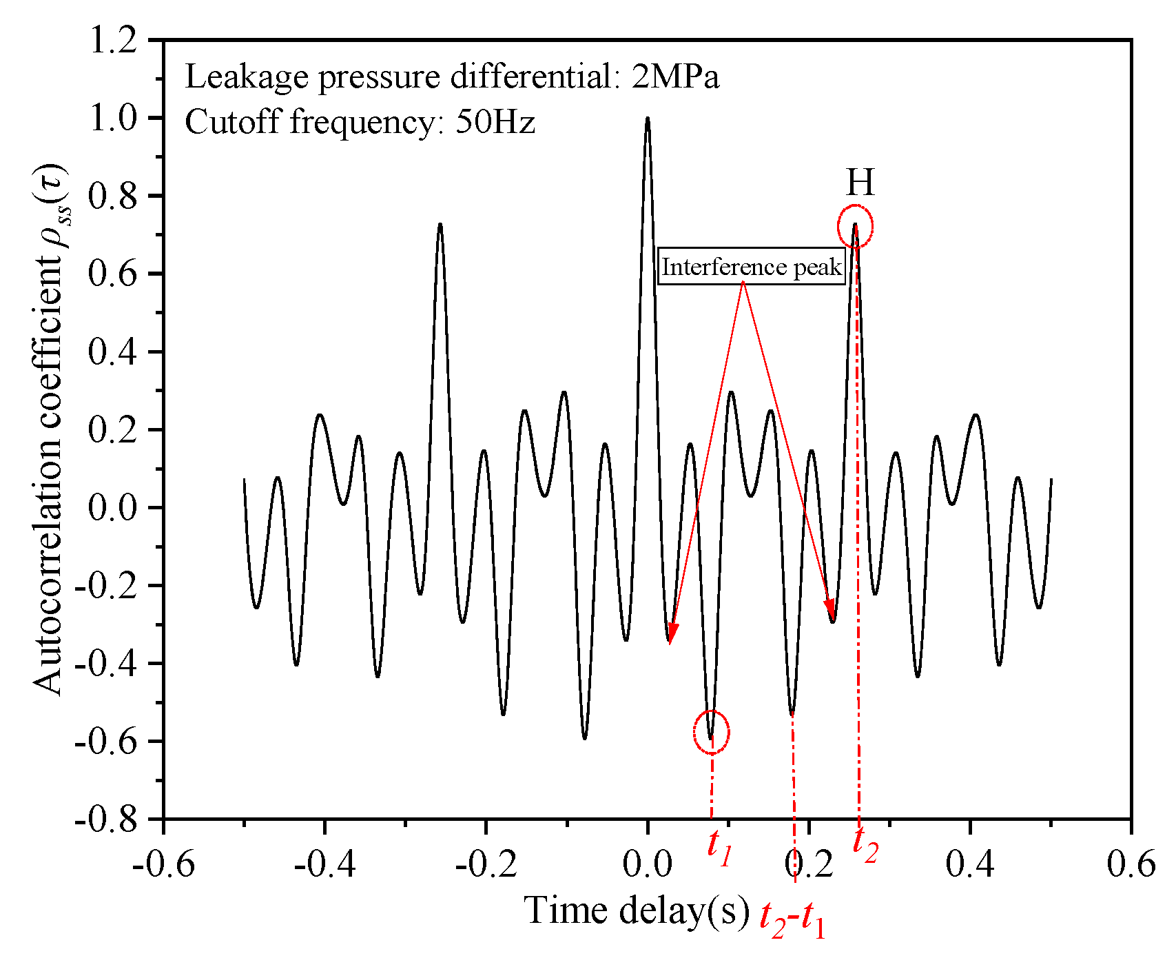
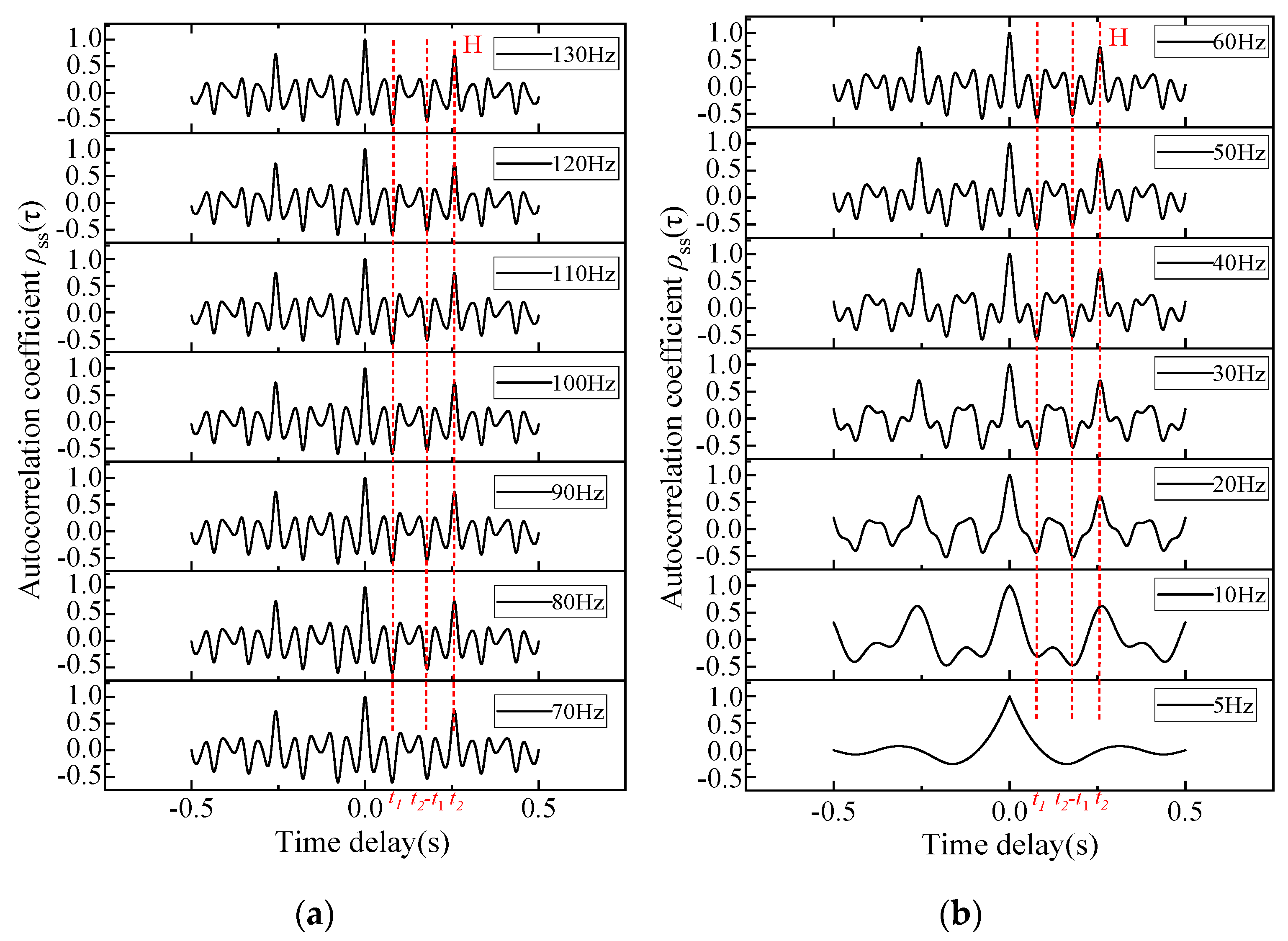
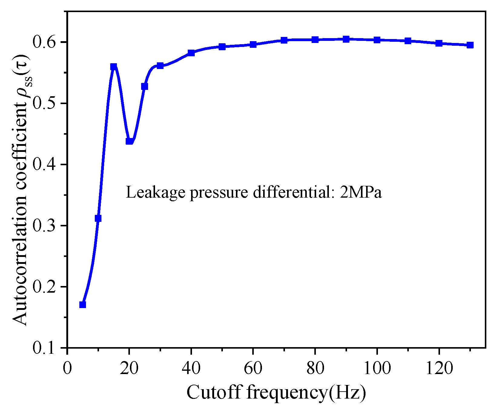
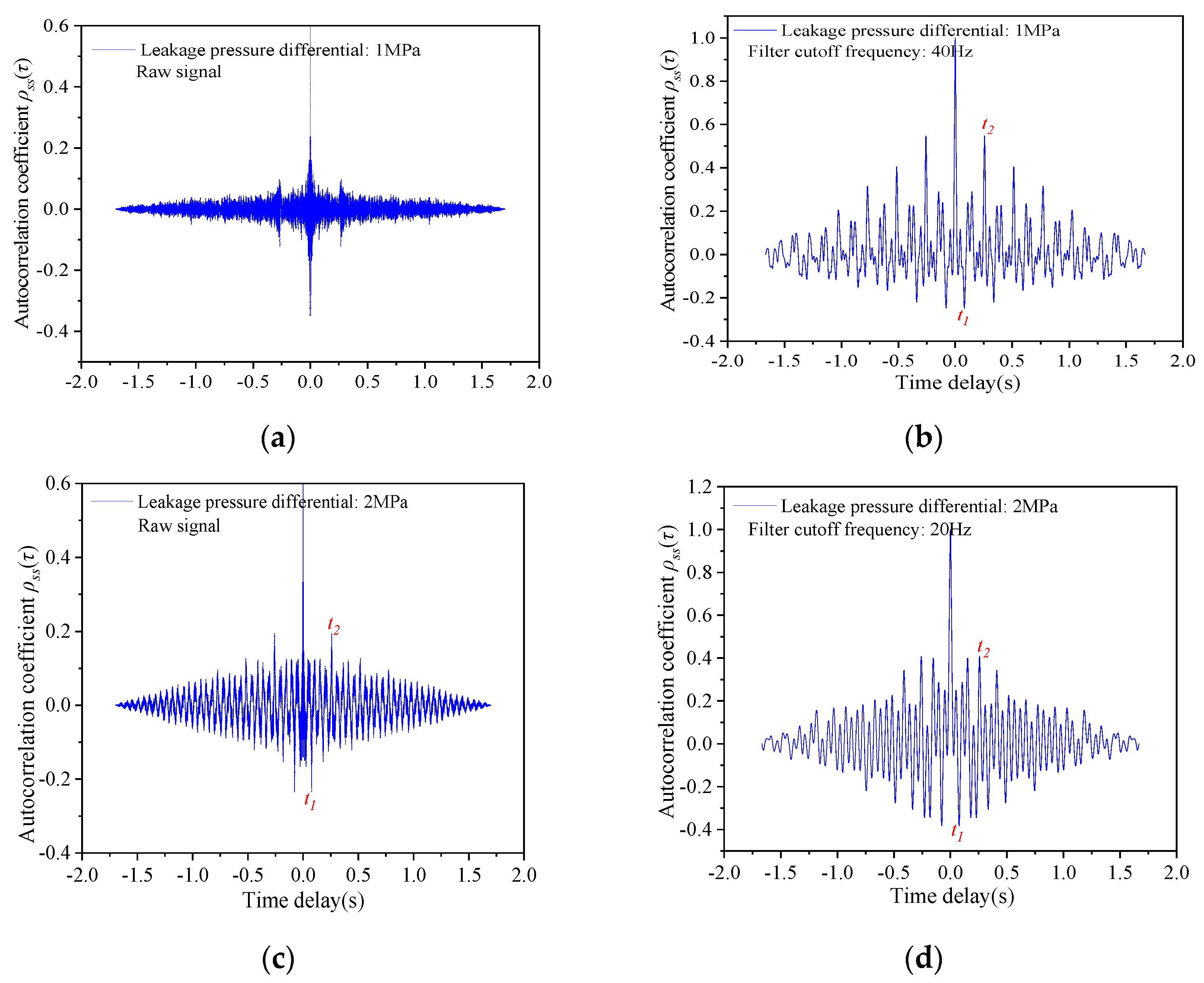
3.1. Effect of Filter Cutoff Frequency on Characteristic Peaks

Leakage acoustic waves represent a type of broadband noise, with the energy of wellhead annular detection signals primarily concentrated in the 1–130 Hz frequency band [24]. Consequently, this study focuses on analyzing the autocorrelation coefficients of leakage acoustic waves within this specific frequency range.

Among Bessel, Chebyshev, and Butterworth filters, the Butterworth filter demonstrates the flattest frequency response within the passband, thereby minimizing distortion of the original signal by electronic filtering. Thus, the Butterworth filter is selected for this study [25,26,27,28]. Additionally, autocorrelation processing of the acoustic signal effectively suppresses random noise.

Figure 5 presents the autocorrelation coefficient curves of leakage acoustic waves under different cutoff frequencies. Key observations include:

• Interference Peak Reduction: Lowering the filter cutoff frequency effectively eliminates interference peaks, indicating that leakage acoustic wave energy is predominantly distributed in the low-frequency range, while random noise exhibits minimal low-frequency components;
• Trade-off in Frequency Selection: As shown in Figure 5b, excessively low cutoff frequencies cause the characteristic peak timings to deviate from theoretical values or even disappear entirely. This demonstrates that an arbitrarily low cutoff frequency is counterproductive, as it distorts the autocorrelation curve and degrades measurement accuracy.

Figure 6 shows the autocorrelation coefficients of effective characteristic peaks under different cutoff frequencies. As can be seen from the figure, the peak values of effective characteristic peaks gradually increase as the filtering cutoff frequency increases. However, when the cutoff frequency exceeds a certain threshold, the rate of increase in the peak values of effective characteristic peaks significantly slows down or even plateaus. Conversely, if the filtering cutoff frequency is set too low, the amplitude of the characteristic peaks decreases sharply, indicating that the filtered leakage acoustic signal gradually becomes distorted. This undoubtedly increases the difficulty of determining the characteristic time. Therefore, when using acoustic autocorrelation analysis to locate tubing leakage, the selection of the filtering cutoff frequency should prioritize a lower value while ensuring that the signal remains undistorted. Additionally, the leakage depth can be cross-verified by analyzing the relationship between the characteristic times t₁, t₂, and t₂ – t₁. Furthermore, the commonly used annular fluid level detector, which is also based on the acoustic method, can provide the round-trip reflection time of acoustic waves traveling up and down the annulus. This means that the characteristic time t₂ can be determined based on the fluid level detection results.

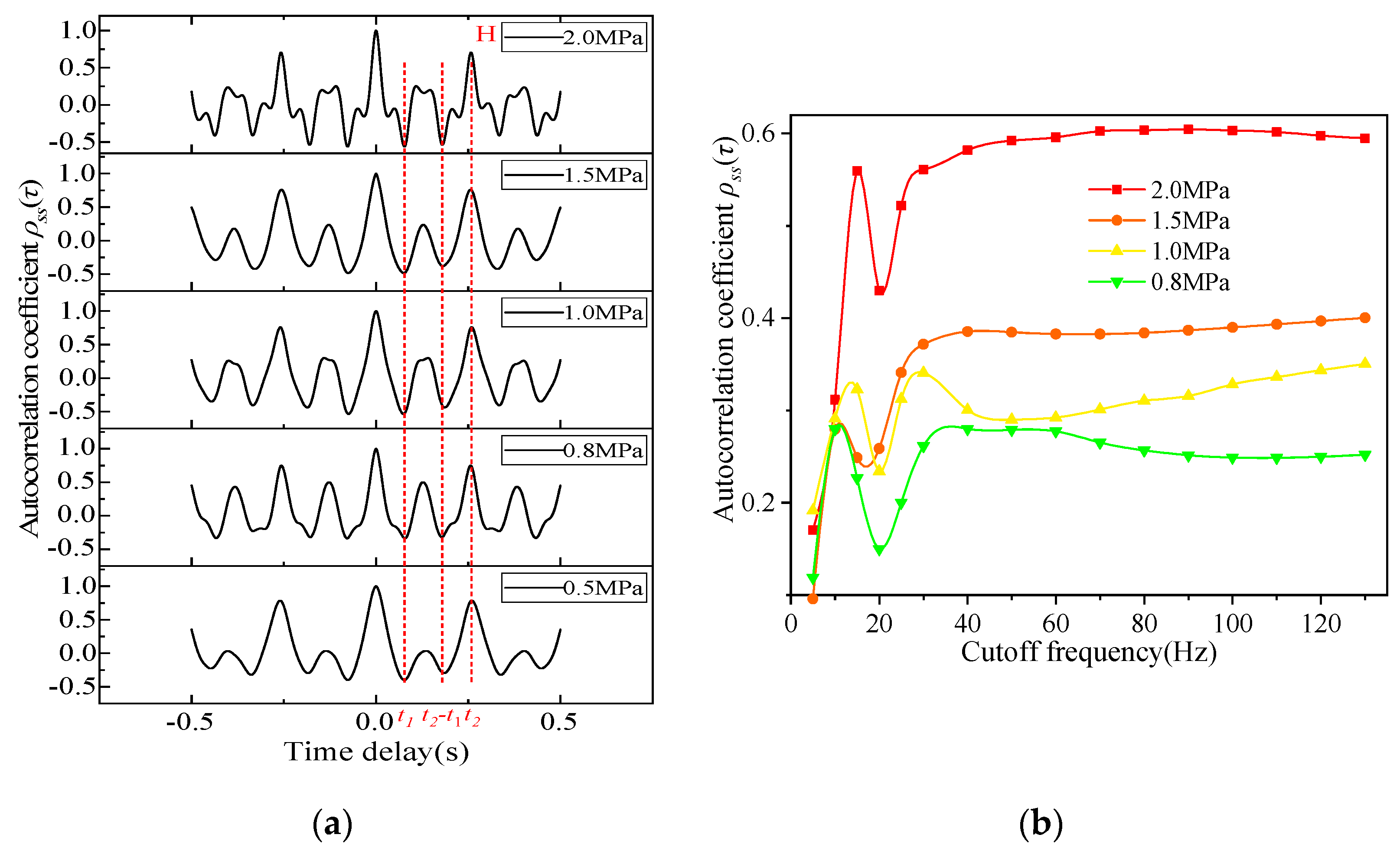
3.2. Influence of Leakage Pressure on Characteristic Peaks

Leakage pressure is a critical factor affecting leakage acoustic signals. As shown in Figure 5, a lower filter cutoff frequency can effectively eliminate interference peaks. Therefore, this section adopts 30 Hz as the cutoff frequency for analyzing leakage acoustic signals.

Figure 7 presents the autocorrelation curves of leakage acoustic signals under different pressures but the same aperture, with the leakage point located 32.84 m from the sensor. From Figure 7a, it can be observed that, under experimental conditions, leakage pressure has almost no effect on the propagation time of leakage acoustic waves within the annulus. It is worth emphasizing that pressure is one of the key factors influencing the gas density in the annulus, thereby affecting the speed of acoustic wave propagation, which in turn determines the time taken for leakage signals to reach the wellhead. However, this does not impact the analysis of characteristic peak amplitudes under different leakage pressures.

Figure 7b displays the peak amplitudes of effective characteristic peaks under varying leakage pressures. The results indicate that the peak amplitude of the characteristic peak increases with increasing leakage pressure, meaning that higher leakage pressure enhances the peak amplitude and improves the distinguishability of the characteristic peak. In field applications, adjusting the pressure difference between the tubing and casing can increase leakage pressure, thereby reducing detection difficulty and improving accuracy.

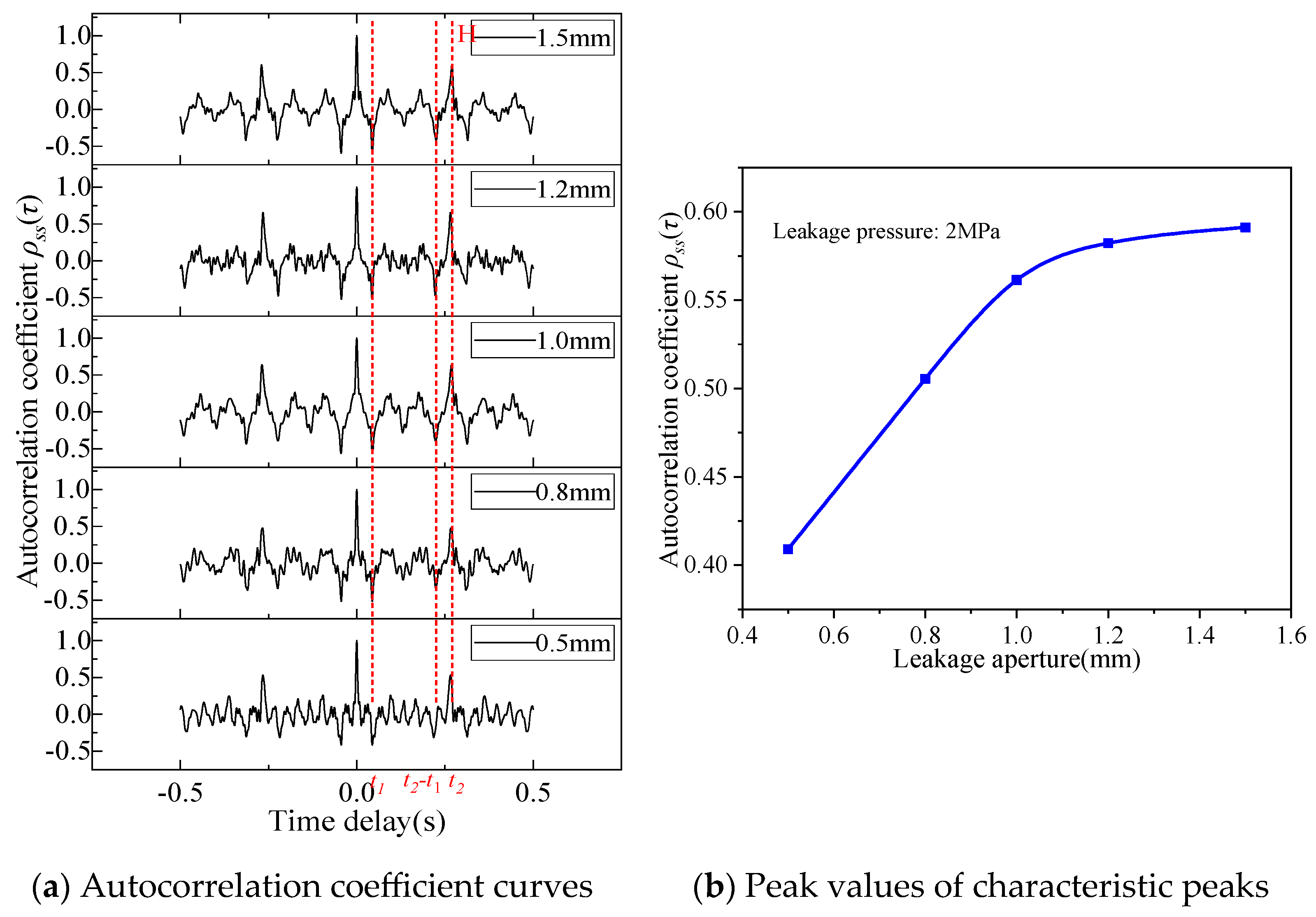
3.3. Influence of Leakage Aperture on Characteristic Peaks

The leakage aperture is another critical factor affecting the characteristics of leakage acoustic waves. Taking a leakage point 39.18 m from the acoustic sensor and a leakage pressure of 2 MPa as an example, Figure 8a shows the autocorrelation coefficient curves of leakage acoustic waves for different aperture sizes. Similar to Figure 7a, the leakage aperture has a negligible influence on the propagation time of leakage acoustic waves within the annulus. The peak values of valid characteristic peaks corresponding to different leakage apertures are presented in Figure 8b.

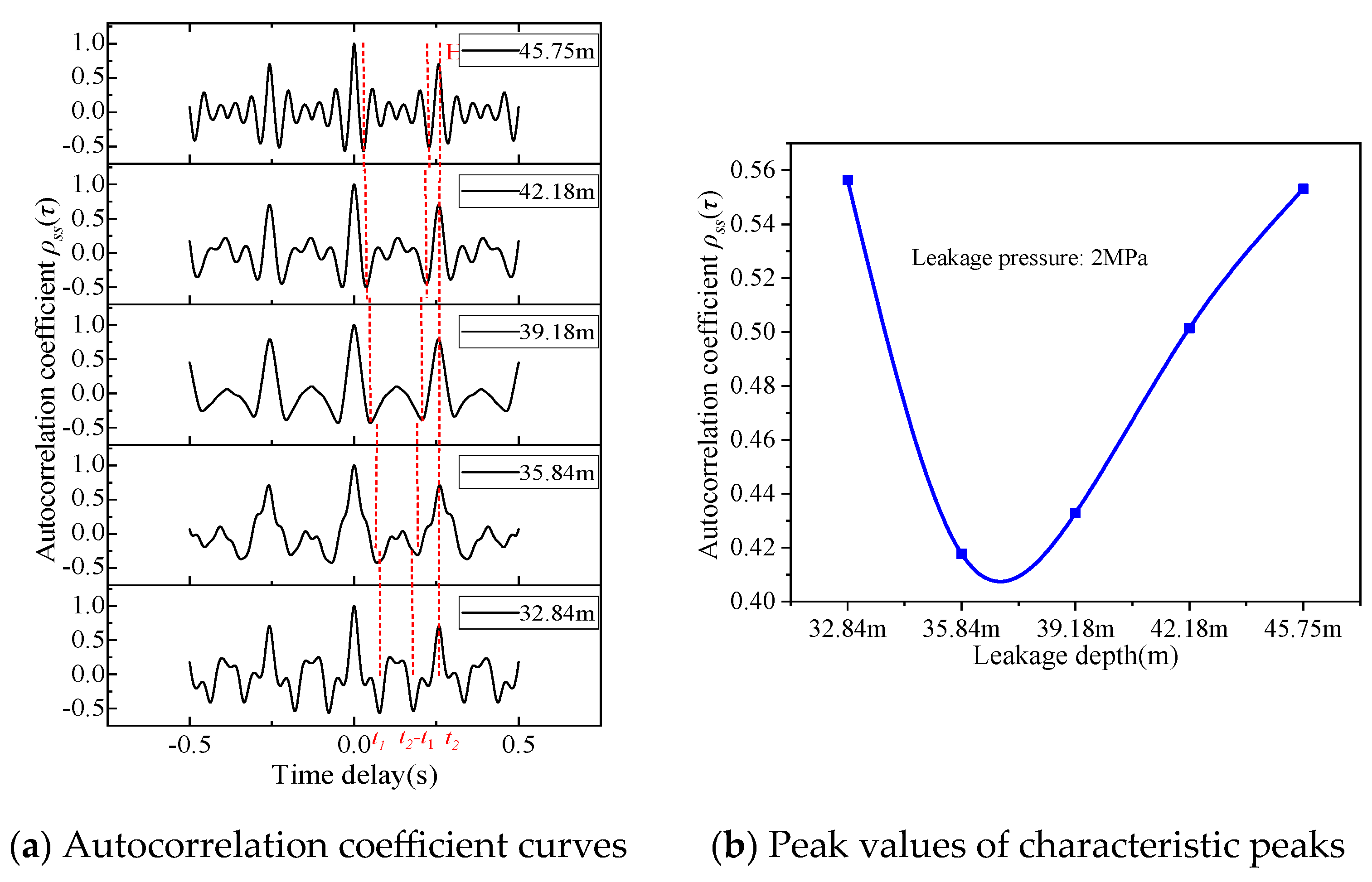
3.4. Influence of Leakage Depth on Characteristic Peaks

Taking a leakage aperture of 1.5 mm and leakage pressure of 2 MPa as an example, Figure 9a displays the autocorrelation coefficient curves of leakage acoustic waves at different leakage depths. As the leakage depth increases, the leakage point becomes closer to the bottom reflection surface, resulting in a smaller characteristic time t₁ and a larger corresponding time difference t₂ − t₁, which aligns with theoretical expectations.

Figure 9b presents the peak amplitudes of valid characteristic peaks at varying leakage depths. Key observations include:

• Nonlinear Relationship: No evident linear correlation exists between leakage depth and the autocorrelation coefficient magnitude of leakage acoustic waves;
• Attenuation Mechanism: Leakage depth primarily affects the signal intensity detected at the wellhead annulus. Acoustic wave attenuation stems mainly from intermolecular friction and absorption, and exhibits a positive correlation with propagation distance [29].

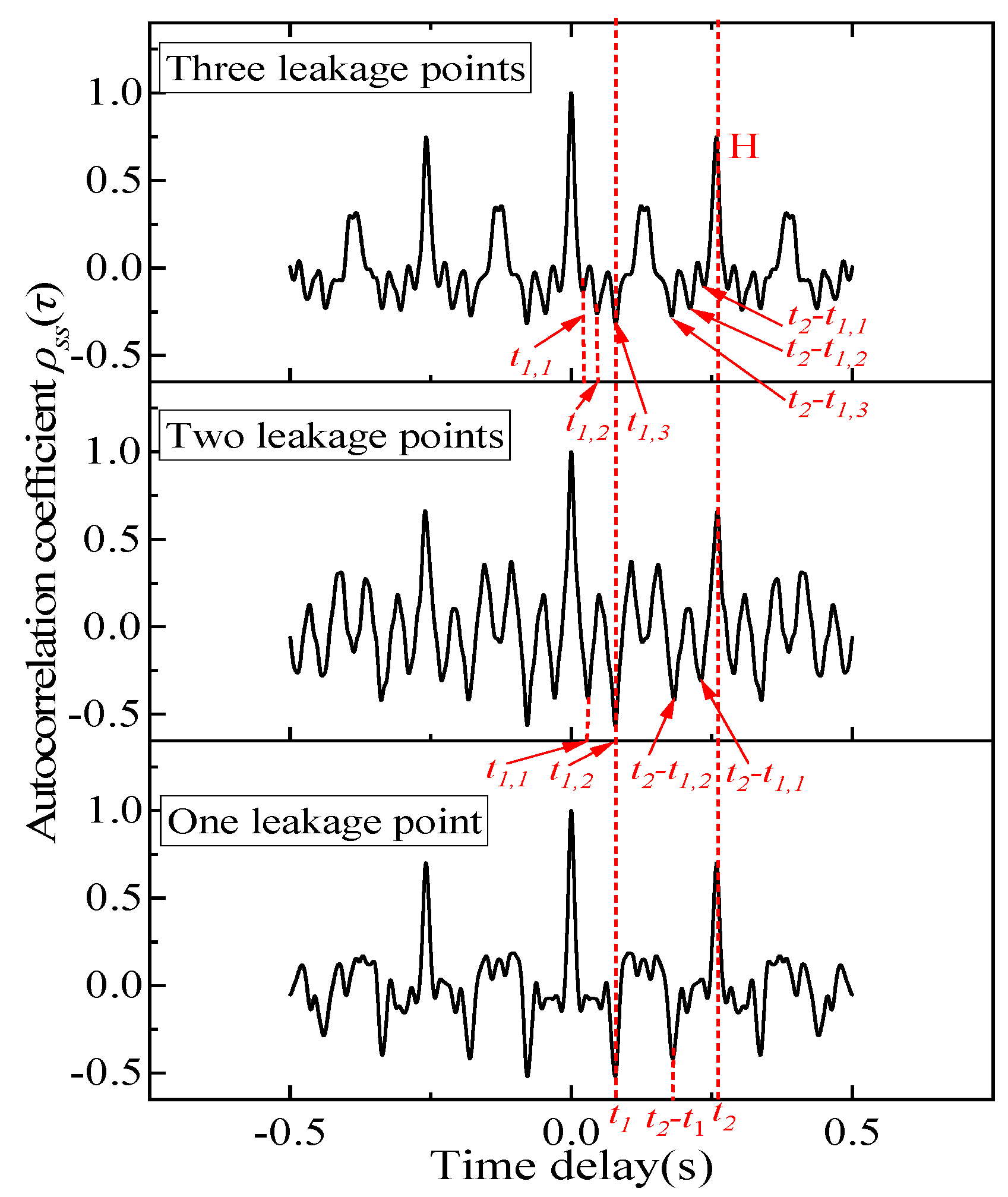
3.5. Effect of Leakage Point Quantity on Characteristic Peaks

Using a leakage aperture of 1.5 mm, leakage pressure of 1.0 MPa, and a cutoff frequency of 30 Hz as test conditions, Figure 10 presents the autocorrelation coefficient curves of leakage acoustic waves under different leakage point quantities. Here, t_1,1, t_1,2, and t_1,3 correspond to the abscissae (horizontal coordinates) of the first, second, and third negative characteristic peaks on the autocorrelation curve. The specific test configurations were:

• Single leakage point: 32.84 m from the acoustic sensor;
• Two leakage points: 39.18 m and 32.84 m from the sensor;
• Three leakage points: 45.75 m, 39.18 m, and 32.84 m from the sensor.

Key findings derived from Equation (1) and Figure 10:

(1) Distance–Peak Relationship: The closer the leakage point is to the sensor, the larger the characteristic time corresponding to the negative peak. Thus, when extracting leakage location characteristics, only the first maximum negative peak on the positive semi-axis needs consideration (left-side analysis).

(2) Multi-Leakage Patterns:

• Negative peaks in the autocorrelation curve increase in pairs with more leakage points;
• The left-side peak of the maximum negative peak may represent true leakage, while the right-side peak is necessarily an interference peak.

(3) Verification Method: The relationship between characteristic times t₁, t₂, and t₂ − t₁ can be used to cross-validate whether left-side peaks correspond to actual leakage points.

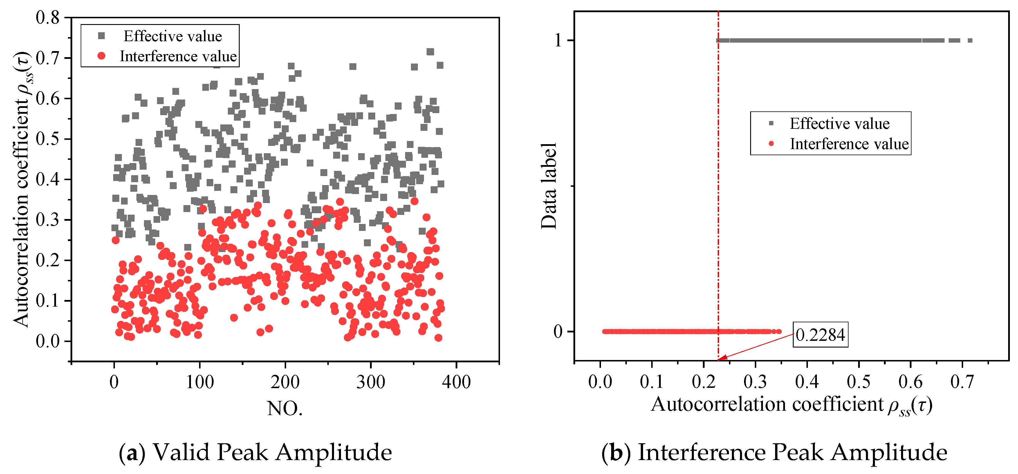
3.6. Comparative Study of Valid Peaks and Interference Peaks

To enhance the accuracy of distinguishing valid characteristic peaks from interference peaks on autocorrelation curves, Figure 11a statistically analyzes approximately 400 sets of absolute peak values under varying operational conditions, categorizing valid peaks (labeled “1”) and interference peaks (labeled “0”). These data are represented in Figure 11b.

Key observations:

(1) Peak Value Overlap: Significant overlap exists between valid and interference peaks, with the minimum valid peak amplitude recorded at 0.2284. This demonstrates that relying solely on a predefined autocorrelation coefficient threshold cannot fully differentiate valid peaks from interference.

(2) Risk-Based Methodology: Adopting the highest-risk principle, all negative peaks with absolute values exceeding 0.2 are preliminarily classified as valid. Subsequent refinement is achieved by integrating prior findings on the effects of:

• Filter frequency;
• Leakage pressure;
• Leakage aperture;
• Leakage depth.

4. Process for Extracting Characteristic Time

Based on the aforementioned research findings, this section proposes a workflow for extracting the characteristic time corresponding to valid peaks on the autocorrelation curve of leakage acoustic signals, as illustrated in Figure 12.

The workflow for extracting characteristic time consists of the following steps:

(1) Pressure Adjustment

Release annular pressure to regulate the pressure difference between the tubing and casing, thereby enhancing the intensity of leakage acoustic signals.

(2) Signal Acquisition and Processing

Capture acoustic signals within the annulus under varying pressure differentials and perform autocorrelation processing on the signals.

(3) Frequency Optimization

Plot autocorrelation coefficient curves under different filter cutoff frequencies.

• Criterion: Select the lowest possible cutoff frequency without signal distortion, typically no lower than 10 Hz.

(4) Peak Validation and Time Extraction

Extract characteristic time corresponding to peaks that satisfy:

• Absolute autocorrelation coefficient > 0.2;
• Consistent presence across curves under different:

  ♦

  Pressure differentials;

  ♦

  Filter cutoff frequencies.

Taking a leakage point 32.84 m from the acoustic sensor as an example, with a signal sampling frequency of 30 kHz and an annular length of 46.2 m, Equations (1) and (2) yield theoretical time delays of approximately t1 = 0.0786 s for the leakage location and t2 = 0.2717 s for the annular length.

Figure 13 displays the autocorrelation coefficient curves of leakage acoustic waves under different cutoff frequencies and pressure differentials. Key observations include:

(1) Pressure Differential Effects: Comparing Figure 13a,c, increasing the leakage pressure differential significantly amplifies the autocorrelation curve amplitude and enhances the discernibility of characteristic times.

(2) Frequency Filtering Effects: Across all subfigures, reducing the filter cutoff frequency:

• Effectively eliminates interference peaks to the left of the first maximum negative peak on the positive semi-axis;
• Ensures the amplitude of characteristic peaks corresponding to leakage locations consistently exceeds 0.2;
• Achieves accurate extraction of leakage position characteristic times.

5. Conclusions

The main points and conclusions of this study are as follows:

(1) Based on experimental data, two key factors affecting the extraction of acoustic characteristic time for leakage were identified: the filter cutoff frequency and the peak amplitude of characteristic peaks in the autocorrelation curve. The appropriate cutoff frequency range is 10–130 Hz, and only characteristic peaks with an absolute value of negative peaks in the autocorrelation coefficient curve greater than 0.2 can be considered as valid peaks generated by leakage.

(2) A procedure for extracting the characteristic time corresponding to leakage location was proposed: Under the premise that the absolute value of characteristic peak coefficients exceeds 0.2 and the peaks are common in the autocorrelation curves under different leakage pressure differentials and filter cutoff frequencies, the corresponding characteristic time should be extracted.

References

1. Available online: https://www.iea.org/reports/gas-market-report-q1-2025 (accessed on 9 March 2025).
2. Hachem, K.E.; Kang, M. Reducing oil and gas well leakage: A review of leakage drivers, methane detection and repair options. Environ. Res. Infrastruct. Sustain. 2023, 3, 012002. [Google Scholar] [CrossRef]
3. Aljameel, S.S.; Alabbad, D.A.; Alomari, D.; Alzannan, R.; Alismail, S.; Alkhudir, A.; Aljubran, F.; Nikolskaya, E.; Rahman, A.-U. Oil and Gas Pipelines Leakage Detection Approaches: A Systematic Review of Literature. Int. J. Saf. Secur. Eng. 2024, 14, 773–786. [Google Scholar] [CrossRef]
4. Zou, X.; Wang, T.; Chen, J.; Liao, Y.; Hu, H.; Song, H.; Yang, C. High-precision monitoring and point location optimization method of natural gas micro-leakage in the well site of salt cavern gas storage. Gas Sci. Eng. 2024, 124, 205262. [Google Scholar] [CrossRef]
5. Zhang, B.; Pan, Z.; Cao, L.; Xie, J.; Chu, S.; Jing, Y.; Lu, N.; Sun, T.; Li, C.; Xu, Y. Measurement of wellbore leakage in high-pressure gas well based on the multiple physical signals and history data: Method, technology, and application. Energy Sci. Eng. 2024, 12, 4–21. [Google Scholar] [CrossRef]
6. Jing, Y.; Wang, T.; Zhang, B.; Zheng, Y.; Li, X.; Lu, N. Safety Risk Analysis of Well Control for wellbore with sustained annular pressure and Prospects for Technological Development. Chem. Technol. Fuels Oils 2025, 61, 1676–1685. [Google Scholar] [CrossRef]
7. Sun, T.; Zhang, Z.; Zhang, Y.; Ma, Y.; Liu, H.; Zhang, Q.; Zhang, B. Enhanced Heat Transfer of Variable Pitch Helical BafflePlate Orifice Plate Type Heater for Downhole In-Situ OilShale Extraction. Phys. Fluids 2025, 37, 057110. [Google Scholar] [CrossRef]
8. Shao, S.R.; Hu, H.; Yang, Z.X.; Tan, P. Quantitative Evaluation of Controlling Factors of Nonuniform Production in Deep Shale Gas Based on Optic Fiber Logging Technology. In Proceedings of the ARMA US Rock Mechanics/Geomechanics Symposium, Golden, CO, USA, 23–26 June 2024. [Google Scholar]
9. Chen, S.; You, H.; Xu, J.; Wei, M.; Xu, T.; Wang, H. Leakage monitoring of carbon dioxide injection well string using distributed optical fiber sensor. Pet. Res. 2025, 10, 166–177. [Google Scholar] [CrossRef]
10. Jiang, C.; Zhao, W.; Yu, M.; Zhang, K. A Model-Based Systematic Innovative Design for Sonic Logging Instruments in Natural Gas Wells. Sensors 2024, 24, 6087. [Google Scholar] [CrossRef] [PubMed]
11. Liu, K.; Zakharova, N.; Adeyilola, A.; Gentzis, T.; Carvajal-Ortiz, H.; Fowler, H. Understanding the CO2 adsorption hysteresis under low pressure: An example from the Antrim Shale in the Michigan Basin: Preliminary observations. J. Pet. Sci. Eng. 2021, 203, 108693. [Google Scholar] [CrossRef]
12. Liu, D.; Fan, J.C.; Wu, S.N. Acoustic Wave-Based Method of Locating Tubing Leakage for Offshore Gas Wells. Energies 2018, 11, 3454. [Google Scholar] [CrossRef]
13. Donoho, D.L. De-noising by soft-thresholding. IEEE Trans. Inf. Theory 1995, 41, 613–627. [Google Scholar] [CrossRef]
14. Heilbronner, R.P. The autocorrelation function: An image processing tool for fabric analysis. Tectonophysics 1992, 212, 351–370. [Google Scholar] [CrossRef]
15. Zhang, M.; Wen, S.P. Applied Numerical Analysis, 4th ed.; Petroleum Industry Press: Beijing, China, 2012; pp. 211–228. ISBN 978-7-5021-9201-3. [Google Scholar]
16. Speed of Sound in Natural Gas and Other Related Hydrocarbon Gases; AGA Report No. 10; AGA XQ0310; American Gas Association: Washington, DC, USA, 2003; pp. 12–17.
17. Coquelet, C.; Chapoy, A.; Richon, D. Development of a new alpha function for the Peng–Robinson equation of state: Comparative study of alpha function models for pure gases (natural gas components) and water-gas systems. Int. J. Thermophys. 2004, 25, 133–158. [Google Scholar] [CrossRef]
18. Izgec, B. Transient Fluid and Heat Flow Modeling in Coupled Wellbore/Reservoir Systems. Ph.D. Thesis, Texas A&M University, College Station, TX, USA, May 2008. [Google Scholar]
19. Lin, J.; Xu, H.L.; Shi, T.H.; Zou, A.Q.; Mu, A.L.; Guo, J.H. Downhole multistage choke technology to reduce sustained casing pressure in a HPHT gas well. J. Nat. Gas Sci. Eng. 2015, 26, 992–998. [Google Scholar]
20. Sagar, R.; Doty, D.R.; Schmidt, Z. Predicting temperature profiles in a flowing well. SPE Prod. Eng. 1991, 6, 441–448. [Google Scholar] [CrossRef]
21. Hasan, A.R.; Kabir, C.S. Wellbore heat-transfer modeling and applications. J. Pet. Sci. Eng. 2012, 86–87, 127–136. [Google Scholar] [CrossRef]
22. Xu, R. Analysis of Diagnostic Testing of Sustained Casing Pressure in Wells. Ph.D. Thesis, Louisiana State University, Baton Rouge, LA, USA, 2002. [Google Scholar]
23. Hasan, A.R.; Kabir, C.S. Heat transfer during two-phase flow in wellbores: Part I—Formation temperature. In Proceedings of the 66th Annual Technical Conference and Exhibition of the Society of Petroleum Engineers, Dallas, TX, USA, 6–9 October 1991; pp. 469–478. [Google Scholar]
24. Zhang, X.M.; Fan, J.C.; Wu, S.N.; Liu, D. A novel acoustic liquid level determination method for coal seam gas wells based on autocorrelation analysis. Energies 2017, 10, 1961. [Google Scholar] [CrossRef]
25. Liu, D.; Chun, F.J.; Jie, L.S.; Yu, W.C.; Wei, L.Z.; Li, F.Z. Experimental Research on the Location of Multiple Leaks in Downhole Tubing of Gas Wells. China Saf. Sci. J. 2018, 14, 6. [Google Scholar]
26. Mo, J. Research on Different Filtering Algorithms Based on Adaptive Noise Cancellation System. Master’s Dissertation, Yunnan Normal University, Kunming, China, 2014. [Google Scholar]
27. Heng, P. Research on Generalized Chebyshev Lossy Filters. Master’s Dissertation, University of Electronic Science and Technology, Chengdu, China.
28. Zhang, Y. Synthesis of the Coupling Matrix for Generalized Chebyshev Bandpass Filters. Master’s Dissertation, Anhui University, Hefei, China, 2016. [Google Scholar]
29. Liu, Y. Research on Key Issues of Butterworth Filters and Single-Phase Phase-Locked Loops. Master’s Dissertation, Huazhong University of Science and Technology, Wuhan, China, 2016. [Google Scholar]
Figure 1. Schematic of acoustic wave propagation path for tubing leakage. (a) Diagram of tubing leakage detection. (b) Simplified propagation path of leakage acoustic waves.
Processes 13 01708 g001
Figure 2. Autocorrelation coefficient curves of acoustic signals.
Processes 13 01708 g002
Figure 3. Radial heat transfer and computational model of the wellbore.(a) wellbore radial heat transfer model (b) wellbore calculation model.
Processes 13 01708 g003
Figure 4. Autocorrelation coefficient curve of the acoustic signal.
Processes 13 01708 g004
Figure 5. Autocorrelation coefficient curves under different cutoff frequencies. (a) Cutoff frequency range: 70 Hz to 130 Hz. (b) Cutoff frequency range: 5 Hz to 60 Hz.
Processes 13 01708 g005
Figure 6. Autocorrelation coefficients of valid characteristic peaks under different cutoff frequencies.
Processes 13 01708 g006
Figure 7. Leakage acoustic wave characteristics under different pressures. (a) Autocorrelation coefficient curves. (b) Peak values of characteristic peaks.
Processes 13 01708 g007
Figure 8. Leakage acoustic wave characteristics under different aperture sizes.
Processes 13 01708 g008
Figure 9. Autocorrelation coefficient curves and characteristic peak amplitudes at different leakage depths.
Processes 13 01708 g009
Figure 10. Autocorrelation coefficient curves of leakage acoustic waves under varying numbers of leakage points.
Processes 13 01708 g010
Figure 11. Valid and interference peak amplitudes of autocorrelation curve characteristic peaks under different operating conditions.
Processes 13 01708 g011
Figure 12. Characteristic time extraction process.
Processes 13 01708 g012
Figure 13. Autocorrelation coefficient curves of leakage acoustic waves under different cutoff frequencies and pressure differentials.(a) The leakage pressure difference is the autocorrelation coefficient curve of 1 MPa original signal, (b) The leakage pressure difference is the autocorrelation coefficient curve of 1 MPa filter cut-off frequency of 40 Hz, (c) The leakage pressure difference is the autocorrelation coefficient curve of 2 MPa original signal, (d) The leakage pressure difference is the autocorrelation coefficient curve of 2 MPa filter cut-off frequency of 20 Hz.
Processes 13 01708 g013
Disclaimer/Publisher’s Note: The statements, opinions and data contained in all publications are solely those of the individual author(s) and contributor(s) and not of MDPI and/or the editor(s). MDPI and/or the editor(s) disclaim responsibility for any injury to people or property resulting from any ideas, methods, instructions or products referred to in the content.