Article

Modeling and Optimization of an Integrated Energy Supply in the Oil and Gas Industry: A Case Study of Northeast China

1
State Key Lab of Power Systems, Department of Energy and Power Engineering, Tsinghua University, Beijing 100084, China
2
Research Institute of Petroleum Exploration and Development, Beijing 100083, China
*
Author to whom correspondence should be addressed.
These authors contributed equally to this work.
Processes 2025, 13(5), 1512; https://doi.org/10.3390/pr13051512
Submission received: 13 April 2025 / Revised: 8 May 2025 / Accepted: 13 May 2025 / Published: 14 May 2025
(This article belongs to the Special Issue Advanced Technologies of Renewable Energy Sources (RESs))

Abstract

:
The oil and gas industry has large and constant power and heat loads and usually ownership of land resources near oil and gas production, providing opportunities for onsite integration of renewable energy. In the future, a possible decrease in reliable and affordable electricity production capability by the power grid, mainly due to the penetration of intermittent renewable energy, makes seeking an alternative energy supply a wise choice for the oil and gas industry. Foreseeable carbon emission costs also drive the oil and gas industry to a less carbon-intensive way of production. However, it is not yet clear whether it is economically viable for the integration of renewable energy in the oil and gas industry. In this work, we propose a modeling and optimization framework for conceptual planning and the operation of an oilfield’s energy system, where energy demands—heat and power in particular, are supposed to be met by an integrated energy supply including both fossil fuels and renewable energy. Herein, an oilfield in Northeast China has been then taken as a case study. The results indicate that under current conditions with no power purchase limits, integrating renewable energy is not economically viable. As the power purchase limits the decrease by a certain threshold, renewable energy integration becomes essential for maintaining a stable power supply, with renewable energy capacity reaching 35% in a self-sufficient microgrid configuration. Similarly, as electricity prices rise, the deployment of renewable energy begins to exhibit economic viability at 1.5 times the current electricity price. Independent microgrids show better economic resilience compared to grid-dependent systems under rising electricity prices. When carbon prices increase, the heat electrification transformation for microgrids achieves a cost inflection point at USD 76.4 per tonne, resulting in overall cost reductions. These findings emphasize the importance of flexible, renewable energy-driven energy systems in cost-effective decarbonization and energy stability, providing insights for optimizing oilfield energy systems and supporting China’s carbon neutrality goals.

1. Introduction

The oil and gas industry plays a key role in the global transition to a low-carbon future [1]. This transition requires the reduction of greenhouse gas emissions and alignment with sustainable development goals [2]. In China, the price of carbon emission permits (CEA) in the national carbon market increased by 97% from USD 6.47/tonne in 2021 to a peak of USD 14.67/tonne on 13 November 2024 [3,4]. This continuously rising carbon price imposes significant financial pressure on high-emission industries such as oil and gas, highlighting the urgency of adopting low-carbon technologies to mitigate rising costs and ensure economic viability [5,6]. However, the industry’s severe reliance on grid electricity and fossil fuel consumption poses major obstacles to decarbonization [7,8].
Oilfields, characterized by their large and stable demand for electricity and heat, require a reliable energy supply, which puts pressure on traditional grid-based solutions [9]. With the rising penetration of renewable energy in the grid, the grid’s reliability is cause of concern [10]. Moreover, unpredictable weather extremes, geopolitical instability, and energy transition challenges may lead to significant fluctuations in electricity prices. For example, in the European electricity market crisis in December 2024, the wholesale electricity prices in southern Norway soared 20 times, while Germany and Italy experienced unprecedented peaks in electricity prices [11]. These risks expose the oil and gas industry to potential power supply disruptions and rising electricity costs [12,13], necessitating alternative energy solutions to reduce reliance on the grid.
In this context, integrating renewable energy with energy storage provides a promising approach to address these challenges [14]. By utilizing land resources typically available near oilfields, renewable energy technologies can be deployed on-site, reducing the dependence on the power grid and carbon emissions [15]. Furthermore, gas turbines widely used in oilfield power systems can provide rapid response capabilities to balance the intermittency of renewable energy [16], while electrified heat systems can further reduce the use of fossil fuels [17,18]. Such hybrid systems combine the flexibility of natural gas with the sustainability of renewables, potentially stabilizing energy supply and improving environmental performance.
There is a growing body of literature that recognizes the importance of integrating renewable energy in oil and gas operations. Oliveira-Pinto et al. analyzed the integration of solar and wind energy into offshore platforms, demonstrating their potential to enhance operational sustainability [19]. This study underscores a vital pathway for decarbonizing remote offshore energy systems. Similarly, Hartmann et al. highlighted the benefits of combining natural gas with renewable energy in oilfield systems. Their work importantly shows that such hybrid systems can effectively manage the intermittency of renewable energy, particularly by leveraging readily available natural gas resources within oilfields [20]. This approach offers a pragmatic strategy for oilfields to transition towards cleaner energy portfolios while maintaining operational reliability.
Some studies have investigated hybrid energy systems to improve energy efficiency and reduce emissions. Huang et al. examined how natural gas power generation can complement renewable energy sources to stabilize grids and improve the economic feasibility of decarbonization initiatives [16]. Rafiee and Khalilepour systematically investigated renewable energy adoption in oil–gas supply chains. They particularly emphasized the technical–economic feasibility of combining concentrated solar power with steam generation for tertiary recovery, and wind energy for offshore platform operations. These integrations address both energy intensity challenges in mature fields and remote operational constraints [21]. Furthermore, studies like Zhong and Bazilian’s analysis of international oil companies’ renewable investments reveal strategic approaches including solar-enhanced oil recovery and offshore wind development. Their research highlights how these integrations aim to address decarbonization while leveraging existing operational expertise [22]. Although these studies offer promising directions for oil and gas decarbonization, they lack quantitative methods and recommendations for configuring renewable energy and storage systems, and they do not validate economic practicality through theoretical models and case studies.
Economic and policy dimensions of renewable energy integration have also been extensively studied. Hartmann et al. analyzed the impact of regulatory pressures and environmental responsibilities on international oil and gas companies, highlighting how these factors drive renewable energy investment decisions [23]. Choi et al. evaluated how financial incentives and policy mechanisms can foster sustainability within oilfield operations, revealing the economic opportunities and barriers associated with renewable energy adoption [24]. However, these studies have failed to quantitatively evaluate the impact of carbon pricing and electricity market volatility on the operating costs of oil and gas fields. There is insufficient elasticity analysis of the oil and gas field system under the evolving policy framework.
In addition, the oil and gas industry’s critical operations demand continuous electricity and heat supply with uninterrupted energy stability. Current oilfield energy systems typically meet these needs by relying on gas turbines and grid power for electricity, alongside natural gas boilers and gas absorption heat pumps for heat. Although this approach ensures operational reliability, its heavy dependence on fossil fuels leads to high carbon emissions and restricts flexibility in the face of ongoing energy transformation. This reliance on conventional, high-emission systems, coupled with the challenge of maintaining a consistent supply under varying conditions, reveals a significant gap in existing research. Therefore, there is a clear need for an optimization framework designed to secure a continuous, stable, and more sustainable energy supply for oilfields.
This study solves these shortcomings by introducing a novel optimization framework that integrates renewable energy, natural gas, advanced storage technologies, and electrified heating equipment to meet oilfield energy demands. This framework employs a variable temporal resolution model to optimize the capacity of energy equipment and energy supply, considering reliability, low cost, and low emissions. It incorporates rising carbon and electricity prices to ensure economic relevance and mitigates renewable intermittency by enhancing system flexibility. Validated through a real-world case study of an oilfield in Northeast China, the framework quantifies economic and environmental impacts across varied scenarios, bridging the gap between theoretical models and practical applicability to support the oil and gas industry’s transition to carbon neutrality.
This paper is organized as follows: Section 2 defines the problem statement, outlining the design of the proposed energy system to tackle the identified challenges. Section 3 details the methodology, including the optimization model with variable temporal resolution, its objective function, unit constraints, and an adaptive time-series aggregation algorithm. Section 4 presents the Northeast China oilfield case study for validation. Section 5 analyzes the results, comparing installed capacities, costs, and sensitivities to grid power limits, electricity prices, and carbon prices. Section 6 concludes with key findings and implications of low-carbon transitions in the oil and gas sector.

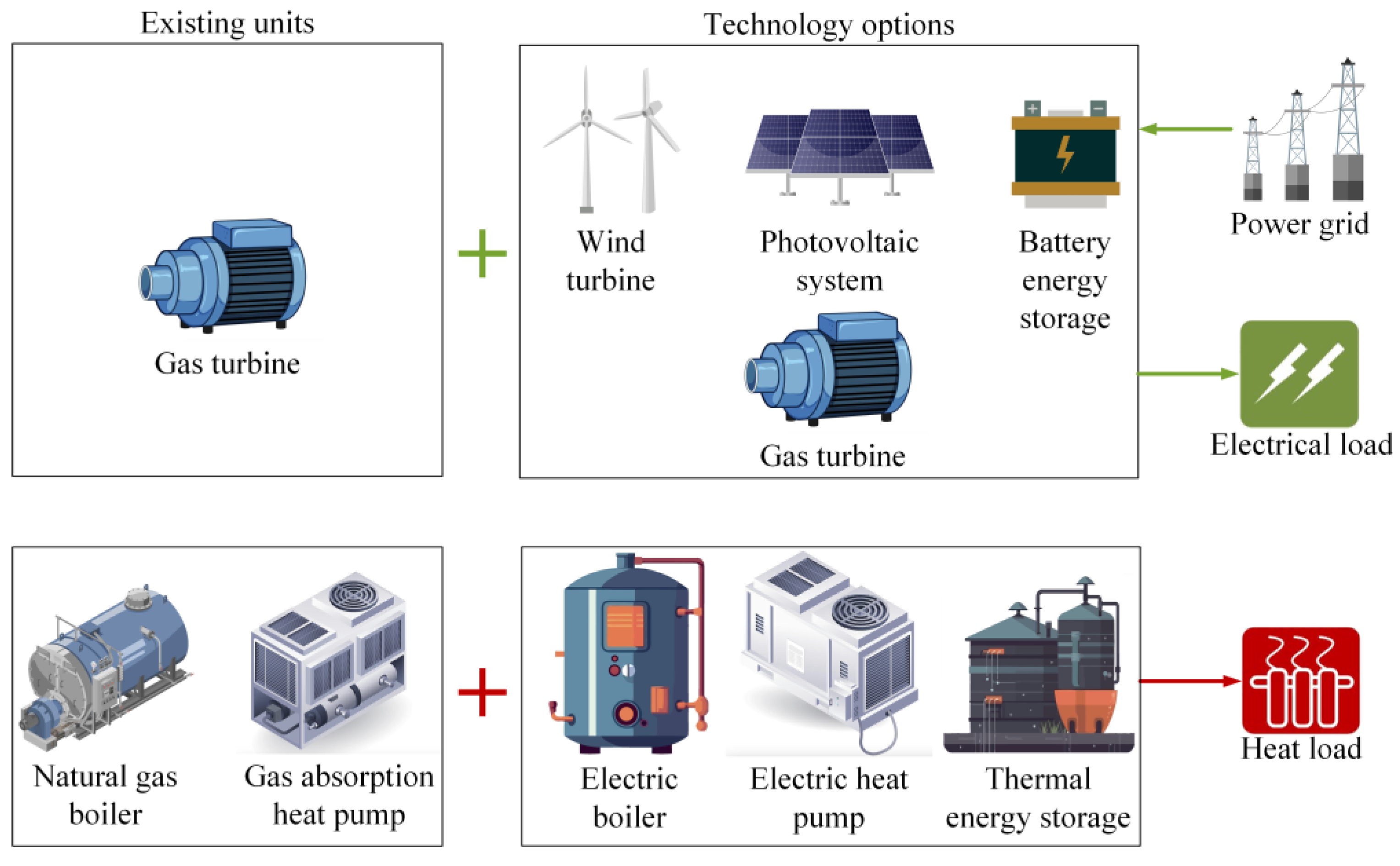
2. System Description

To overcome these limitations described in the Introduction Section, the proposed system integrates multiple advanced energy technologies, including photovoltaic systems, wind turbines, battery energy storage systems, thermal energy storage systems, electric boilers, and electric heat pumps. Wind and solar energy, as the main renewable energy source, significantly reduce the reliance on fossil fuels and lower carbon emissions. The integration of gas turbines and energy storage technology addresses the intermittency and volatility of renewable energy generation, ensuring the reliability and stability of energy supply. Electrification technologies, including electric boilers and heat pumps, further support decarbonization by replacing traditional fossil fuel-based heat systems and improving the utilization of renewable energy.
Technologies incompatible with decarbonization and sustainability goals, such as coal-fired units, are excluded from the system. Similarly, due to the logistics challenges of supplying biomass to remote oilfield locations, biomass boilers have also been omitted. This selection ensures the system focuses on feasible and sustainable technologies, supporting an effective transition to a low-carbon energy system.
Figure 1 illustrates the structure of the proposed integrated renewable energy system. The figure is divided into two parts: the left side represents the existing units, including gas turbines, natural gas boilers, and gas absorption heat pumps. These components are retained to ensure stability and operational reliability. The right side highlights the newly integrated technologies, designed to enhance the system’s sustainability and flexibility. By integrating existing and advanced technologies, the system provides a scalable pathway for oilfields to achieve a reliable, low-carbon energy supply, addressing key challenges while supporting global sustainability objectives.

3. Methodology

This section outlines the methodology for optimizing oilfield energy systems. It includes two main components: an optimization model with variable temporal resolution and an adaptive time-series aggregation algorithm. The optimization model integrates the physical modeling of key energy generation and storage technologies and defines an objective function and a set of constraints to represent the scope of system planning from 2025 to 2060. The adaptive time series aggregation algorithm dynamically adjusts the time resolution, effectively captures the variability of renewable energy production, and improves computing efficiency.

3.1. Optimization Model with Variable Temporal Resolution

3.1.1. Objective Function

The objective of the optimization model is to minimize total annualized costs C total in Equation (1). It includes annualized investment costs C inv , operation and maintenance costs C OM , fuel consumption costs C fuel , electricity purchase costs C net , as well as carbon costs C C O 2 .
C total = C inv + C OM + C fuel + C net + C CO 2
The annualized investment cost is calculated in Equation (2), which takes into account the initial investment, replacement costs, and the residual value over the planning horizon. Investment costs for equipment are modeled to decline over time, reflecting technological advancements and market trends.
C inv = t e c h C initial + k = 1 N replace ( C replace , k C res , k ) A = t e c h p r i c e inv P install 1 + k = 1 N replace ( 1 r t e c h ) t k ( 1 + I ) t k R res ( 1 + I ) t k A t e c h PV , WT , GT , NGB , EB , GAHP , EHP , BESS , TESS
where PV , WT , GT , NGB , EB , GAHP , EHP , BESS , TESS represent photovoltaic systems, wind turbines, gas turbines, natural gas boilers, electric boilers, gas absorption heat pumps, electric heat pumps, battery energy storage systems, and thermal energy storage systems, respectively. r t e c h donates the annual rate of decline in equipment investment costs, specified as 3% for renewable energy [25], 15% for battery energy storage systems [26], and 1% for other units. R res represents the residual value rate, specified as 3%. I is the discount rate, specified as 0.1 [27]. The term A represents the annuity factor, used to annualize the total investment cost over the planning period, considering the time value of money and is calculated using Equation (3).
A = I 1 ( 1 + I ) T plan
where T plan is the total number of years from 2025 to 2060, specified as 35 years.
The annualized operation and maintenance cost, as represented in Equation (4), includes both fixed and variable components. The variable operation and maintenance cost is calculated over each time step, denoted as Δ t , which reflects the temporal granularity of the model. The time step Δ t dynamically adjusts according to the system’s variability, ensuring higher resolution during periods of significant fluctuation and coarser resolution during stable intervals. The adaptation of Δ t directly influences the precision of the operation and maintenance cost calculations by capturing operational dynamics at varying temporal resolutions, which will be discussed in Section 3.2.
C OM = t e c h p r i c e OM , fix , t e c h P install , t e c h + t t e c h p r i c e OM , var , t e c h P t e c h , t Δ t t e c h PV , WT , GT , NGB , EB , GAHP , EHP , BESS , TESS
where p r i c e OM , fix , t e c h denotes the fixed operation and maintenance price per unit of installed capacity for the technology identified by t e c h . P install , t e c h represents the installed capacity. p r i c e OM , var , t e c h denotes the variable operation and maintenance price per unit of operational load for the technology. P t e c h , t represents the operational power output of the technology tech at time t .
The fuel considered in this study is natural gas, and the annualized fuel consumption cost is calculated using Equation (5).
C fuel = t p r i c e gas F gas , t Δ t
where p r i c e gas represents the price of natural gas, and F gas , t denotes the natural gas consumption at time t .
The cost of electricity purchased from the grid is calculated using Equation (6). This cost reflects the total energy procured during the model period, multiplied by the grid price at each time step. It accounts for the electricity demand that cannot be met by on-site generation, ensuring system reliability and stability.
C net = t p r i c e net , t E net , t Δ t
where F gas , t represents the price of grid electricity at time t , and E net , t denotes the amount of electricity purchased from the grid at time t .
The carbon cost shown in Equation (7) represents the economic impact of carbon emissions associated with fuel consumption and grid electricity usage. This cost is determined by the carbon price and the total emissions produced at each time step. By incorporating carbon costs, the model incentivizes lower-emission technologies and promotes a cleaner energy transition.
C CO 2 = t p r i c e CO 2 , t E CO 2 , t Δ t
where p r i c e CO 2 , t represents the carbon price at time t , and E CO 2 , t denotes carbon emissions at time t .

3.1.2. Constraints

The constraints of the model are essential to maintaining the proper functioning of power generation, heat production, and energy storage units, while also enforcing the balance between supply and demand. The following sections provide detailed descriptions of the constraints applied to different units of the system.
  • Photovoltaic Module
The power output of photovoltaic systems is influenced by both irradiance and temperature, reflecting the nonlinear behavior of PV efficiency under varying environmental conditions. The relationship between available PV power and irradiance is described by a linear scaling factor relative to the standard test conditions (STC), as shown in Equation (8) [28]. The efficiency of the PV module is further influenced by temperature deviations from the STC and logarithmic irradiance variations, as outlined in Equation (9) [29]. The actual usable power from the PV system is given by Equation (10).
x PV , avail , t = P PV , avail , t P PV , rated = G t G STC η PV
η PV = η STC 1 β 0 ( T t T STC ) + γ log 10 G t G STC
P PV , use , t = x PV , avail , t P PV , instal P PV , cur , t
where x PV , avail , t represents the availability factor of the PV system at time t , reflecting the proportion of rated power output based on real-time irradiance conditions. G t is the irradiance at time t , normalized by the irradiance at standard test conditions G STC . The efficiency η PV is influenced by the temperature deviation T t T STC , where β 0 represents the temperature coefficient of efficiency. The term γ captures the logarithmic sensitivity of efficiency to irradiance variation. The actual usable power P PV , use , t is determined by multiplying the availability factor by the installed capacity P PV , instal and subtracting curtailed power P PV , cur , t .
2.
Wind Turbine
The wind speed at the hub height of a wind turbine is estimated using the power law relationship, which models the variation in wind speed with height based on the reference wind speed and wind shear coefficient, as shown in Equation (11) [30]. This method accounts for the vertical wind profile and ensures accurate estimation of wind energy potential at different heights. The power output of the wind turbine is determined by a piecewise function of wind speed, as described in Equation (12). No power is generated when the wind speed falls below the cut-in speed v in or exceeds the cut-out speed v out . Between the cut-in and rated wind speeds v rated , the power output follows a quadratic relationship, while full capacity is achieved between v rated and v out [28]. The actual wind power output equals the product of availability factor and installed capacity, minus curtailments, as shown in Equation (13).
v t = v hub h WT h hub α
x WT , avail , t = P WT , avail , t P WT , rated = 0 , 0 v t < v in A 0 + A 1 v t + A 2 v t 2 , v in v t < v rated 1 , v rated v t < v out 0 , v t v out
P WT , use , t = x WT , avail , t P WT , instal P WT , cur , t
where v t represents the wind speed at height t , while v hub denotes the wind speed at the hub height. The term h WT is the height at time t , and h hub refers to the turbine hub height. The exponent α , specified at 0.143, accounts for the wind shear effect. The availability factor, x WT , avail , t , reflects the proportion of rated power available at any given wind speed. Coefficients A 0 , A 1 , and A 2 are derived from the turbine’s power curve and define the quadratic relationship between wind speed and output power. P WT , avail , t and P WT , rated denote the available and rated power output, respectively. P WT , cur , t represents curtailed wind power at time t .
3.
Gas Turbine
The operation of gas turbines in the oilfield energy system is governed by several key constraints to ensure safe and efficient performance. The output power of the gas turbine must remain within its minimum and maximum operational limits, as shown in Equation (14). The operational status of the gas turbine, represented by a binary variable, is constrained by the total installed capacity, which prevents the turbine from exceeding the number of available units, as described in Equation (15). To maintain operational stability and prevent abrupt fluctuations, the ramp rate is limited, restricting the change in power output between consecutive time intervals, as expressed in Equation (16). The fuel consumption of the gas turbine is determined by the output power, efficiency, and the lower heat value (LHV) of the fuel, as illustrated in Equation (17).
o GT , t P GT , min P GT , t o GT , t P GT , max
0 o GT , t n GT , install
r a m p GT , max P GT , t + 1 P GT , t r a m p GT , max
F GT , t = P GT , t η GT L H V gas
where o GT , t denotes the operational state of the gas turbine at time t . P G T , t represents the turbine’s output power, constrained by minimum and maximum limits P GT , min and P GT , max . The total number of operating turbines is governed by n GT , install . The term r a m p GT , max sets the upper bound for permissible changes in turbine output between consecutive time steps. Fuel consumption F GT , t depends on the output power, turbine efficiency η G T , and the fuel’s lower heat value L H V gas .
4.
Heat Generation Units
Natural gas boilers, electric boilers, gas absorption heat pumps, and electric heat pumps are the primary heat generation units in oilfield energy systems. Despite their different operating mechanisms, these units share similar operational constraints regarding on/off status, heat output range, and ramping rates. The key distinction lies in energy consumption calculations: natural gas-fired units consume fuel based on the lower heat value of gas L H V gas , while electric heat units calculate power consumption based on efficiency or coefficient of performance (COP).
The heat output of each unit must remain within its allowable operational range, as shown in Equation (18). The operational status of each unit should not exceed the total number of installed units, which is constrained by Equation (19). To ensure stable and safe operation, the ramping rate is limited by Equation (20).
o i , t Q i , min Q i , t o i , t Q i , max , i N G B , E B , G A H P , E H P
0 o i , t n i , install
r a m p i , max Q i , t + 1 Q i , t r a m p i , max
The fuel or power consumption is determined by the type of heat generation unit. For natural gas boilers and gas absorption heat pumps, fuel consumption is calculated using Equation (21), while electric boilers and electric heat pumps use Equation (22) and Equation (23), respectively.
F i , t = Q i , t η i L H V gas , i N G B , G A H P
P EB , t = Q EB , t η EB
P EHP , t = Q EHP , t C O P EHP
where Q i , t denotes the heat output of unit i at time t , o i , t the number of the unit in operation at time t , and n i , install is the maximum number of installed units. The maximum allowable ramping rate is indicated by r a m p i , max . For natural gas-fired units, F i , t is the fuel consumption, η i is the efficiency, and L H V gas is the lower heat value of the natural gas. In electric heat units, P EB , t and P EHP , t refer to the power consumption of the electric boiler and electric heat pump, respectively, with η EB representing the efficiency of the electric boiler and C O P EHP denoting the coefficient of performance for the electric heat pump.
5.
Energy Storage System
The energy storage system plays a crucial role in balancing energy supply and demand, enhancing system stability, and improving the integration of renewable energy sources. Battery energy storage systems store electrical energy, while thermal energy storage systems store excess thermal energy. Both systems operate within predefined charging and discharging limits to prevent overcharging or excessive depletion. The state of charge for battery energy storage systems S O C and the state of thermal for thermal energy storage systems S O T evolve based on charging and discharging activities, ensuring optimal performance and longevity.
The charging and discharging power of battery energy storage systems must remain within specified limits, as shown in the following constraints [31]:
0 P BESS , char , t P BESS , char , max
0 P BESS , disc , t P BESS , disc , max
Similarly, thermal energy storage systems operate under analogous constraints:
0 Q TESS , char , t Q TESS , char , max
0 Q TESS , disc , t Q TESS , disc , max
The S O C of battery energy storage systems evolves according to the difference between charging and discharging power, accounting for efficiency losses during energy conversion, as shown in Equation (28) [32].
S O C t = S O C t 1 + P BESS , char , t η char P BESS , disc , t η disc Δ t t C A P BESS
Similarly, the S O T of thermal energy storage systems follows an equivalent formulation, representing the thermal energy balance over time as follows:
S O T t = S O T t 1 + Q TESS , char , t η char Q TESS , disc , t η disc Δ t t C A P TESS
The operational S O C and S O T are constrained within allowable limits to ensure safe and reliable operation [31] as follows:
S O C min S O C t S O C max
S O T min S O T t S O T max
where P BESS , char , t and P BESS , disc , t represent the charging and discharging power of the battery storage system at time t , with maximum allowable values of P BESS , char , max and P BESS , disc , max , respectively. Q TESS , char , t and Q TESS , disc , t denote the charging and discharging rates of the thermal storage system, constrained by Q TESS , char , max and Q TESS , disc , max . The terms η char and η disc indicate the charging and discharging efficiencies, while Δ t refers to the time interval. C A P BESS and C A P TESS represent the total capacities of the battery and thermal storage systems. S O C t and S O T t describe the state of charge and state of thermal at time t , with upper and lower bounds defined by S O C max , S O C m i n , S O T max , and S O T min .
6.
Power Balance
The power balance constraint is essential for maintaining stable and reliable operation of integrated energy systems, ensuring that the total power generated meets the total power consumed at each time step. The system’s power generation primarily consists of outputs from gas turbines, WT, PV, discharges from battery energy storage systems, as well as net power purchase from the grid. Conversely, power consumption is driven by electrical loads, the charging of battery energy storage systems, and the operation of electric boilers and electric heat pumps. The power balance constraint for the system is represented in Equation (32).
P GT , t + P WT , use , t + P PV , use , t + P BESS , disc , t + P grid , t = P load , t + P BESS , char , t + P EB , t + P EHP , t
where the left-hand side of Equation (32) represents the total power supply, including the outputs from the gas turbine P GT , t , wind turbine P WT , t , photovoltaic system P PV , t , and battery discharge P BESS , disc , t , as well as the power purchased from the grid P grid , t . The right-hand side reflects the total power consumption, including the electrical load P load , t , battery charging power P BESS , char , t , and the power consumed by the electric boiler P EB , t and electric heat pump P EHP , t .
7.
Heat Balance
The heat balance constraint is fundamental for ensuring the stability and efficiency of the thermal energy system, aligning heat generation with consumption at each operational step. Heat generation stems from units such as natural gas boilers, electric boilers, gas absorption heat pumps, and electric heat pumps, as well as discharges from thermal energy storage systems. On the consumption side, heat is utilized to meet heat loads and charge the thermal energy storage systems for future use. The thermal power balance constraint for the system is expressed in Equation (33).
Q NGB , t + Q EB , t + Q GAHP , t + Q EHP , t + Q TESS , disc , t = Q load , t + Q TESS , char , t
where the left-hand side of Equation (33) represents the total heat supply, encompassing the outputs from the natural gas boiler Q NGB , t , electric boiler Q EB , t , gas absorption heat pump Q GAHP , t , electric heat pump Q EHP , t , and the discharge from the thermal energy storage system Q TESS , disc , t . The right-hand side reflects the heat demand, which includes the heat load Q load , t and the heat used to charge the thermal energy storage systems Q TESS , char , t .

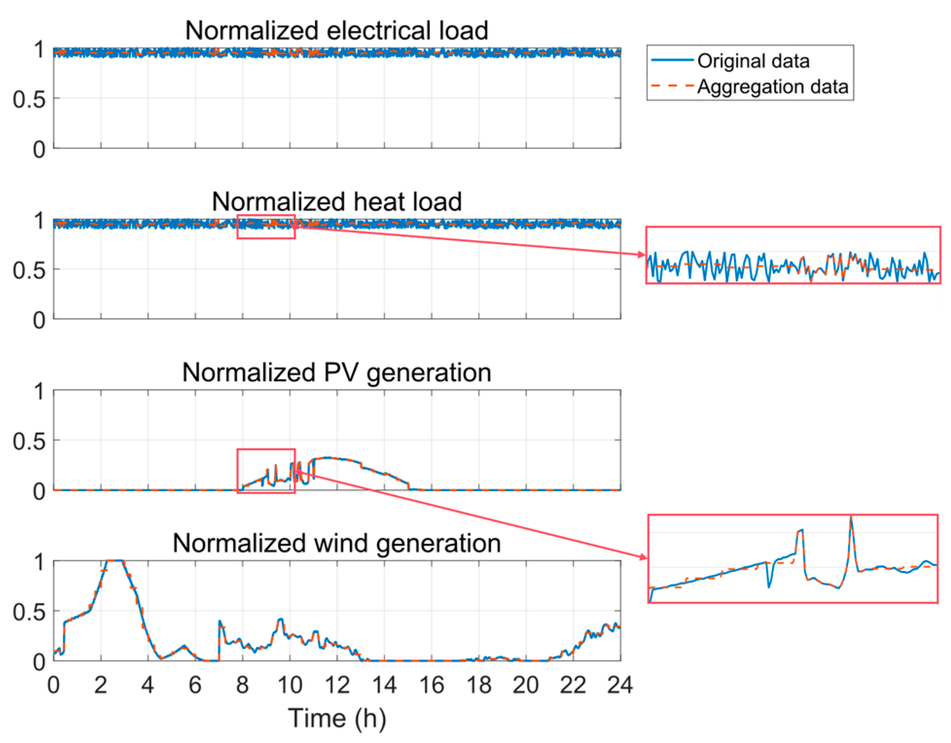
3.2. Adaptive Time-Series Aggregation Algorithm

In energy system modeling, the time resolution is a critical factor affecting computational efficiency and result accuracy. To simplify computation, traditional models usually adopt a fixed time resolution, typically set to once per hour. Although this method reduces computational complexity, it fails to fully capture the drastic fluctuations of renewable energy within an hour [33]. Conversely, employing high-resolution data, such as one-minute intervals, improves the accuracy of modeling these fluctuations but leads to excessive computational burdens, particularly in large-scale energy systems. This trade-off is especially pronounced in oil and gas systems, where the relatively stable electricity and heat demands contrast sharply with the high intermittency of renewable energy generation.
To address this challenge, this study utilizes an adaptive time series aggregation algorithm as part of the variable time resolution model. This algorithm provides an innovative solution by dynamically adjusting the temporal granularity of the input data based on system variability [28]. This algorithm involves identifying variability thresholds in the time series data to dynamically adjust temporal resolution. During periods of low variability, such as stable solar generation under clear weather or consistent night-time energy demand, data points are aggregated into 60 min intervals. In contrast, during periods of high variability, such as rapid changes in wind speed or cloud cover, finer resolutions of 1 min or 15 min are used. By selecting 1 min, 15 min, or 60 min resolutions based on the intensity of fluctuations, this iterative process balances computational efficiency and modeling accuracy by choosing the appropriate resolution.
By incorporating this algorithm into the optimization model, the study achieves several key advantages. Firstly, it effectively reduces the dimensionality of the input data, significantly enhancing computational efficiency. Secondly, the algorithm preserves the accuracy of critical dynamic characteristics by maintaining high-resolution data, such as during peak load fluctuations or rapid changes in renewable generation. Thirdly, it aligns the temporal resolution with the specific characteristics of oilfield energy systems, where stable demand profiles coexist with intermittent renewable energy inputs.

4. Case Study

To develop an optimized planning solution for oilfield energy systems, a case study is conducted on an oilfield located in northern China. This region is characterized by abundant solar and wind resources, making it highly suitable for renewable energy integration. The case study leverages the Variable Temporal Resolution Optimization Model to evaluate the feasibility of incorporating renewable energy and enhancing the existing infrastructure to support the oilfield’s low-carbon transition.

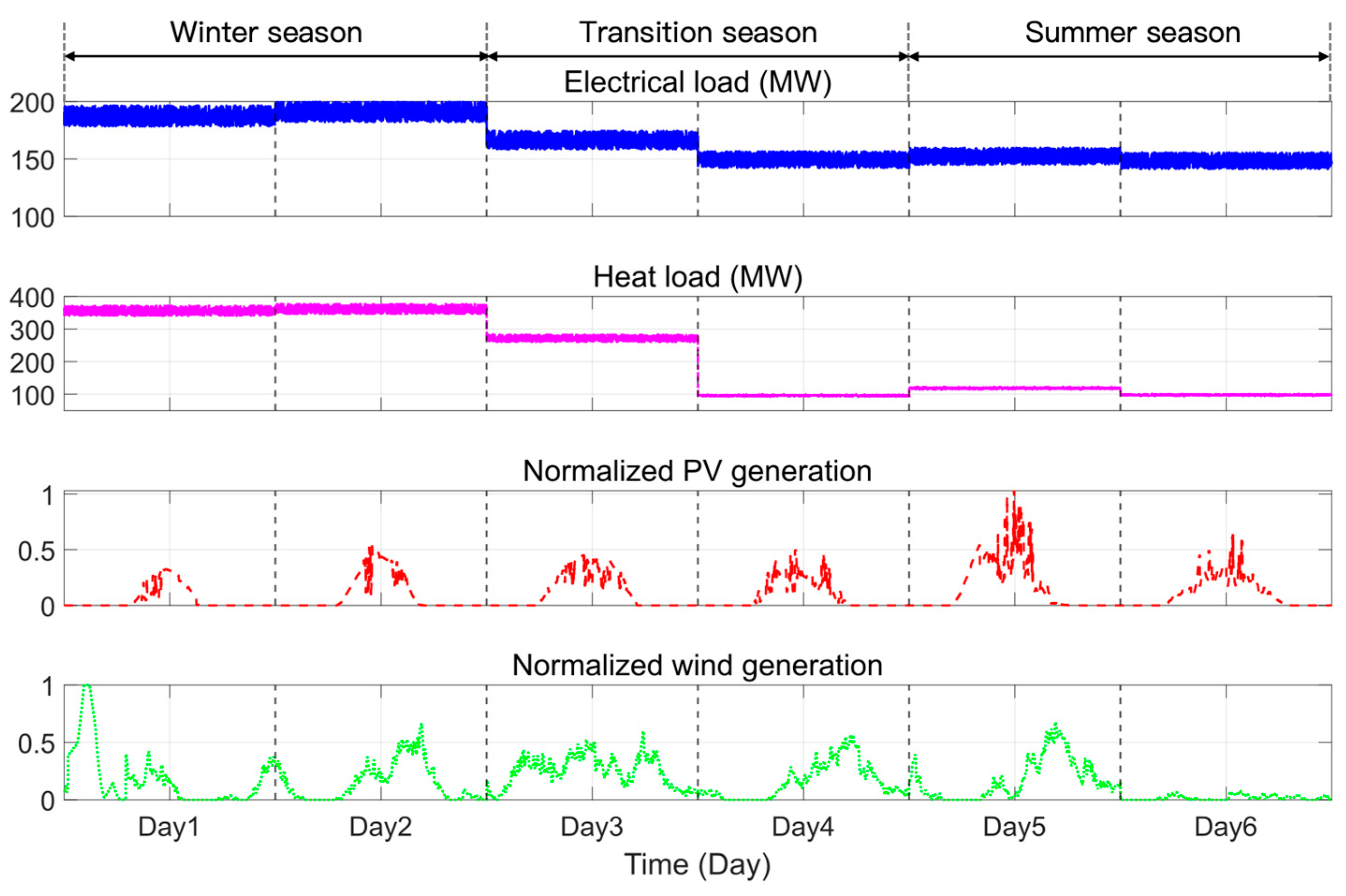
4.1. Model Inputs and Parameter Settings

The existing system layout consists of two 48 MW gas turbines for power supply, three 4 MW gas absorption heat pumps, and thirty-six 10 MW natural gas boilers for heat supply. However, all currently deployed equipment has exceeded its recommended operational lifespan. As a result, it is assumed that starting from the planning baseline year of 2025, all cases will involve a complete replacement of energy equipment. In Case 1, the system configuration adheres to the original layout, updating the aging equipment with equivalent replacements to maintain the same system structure. In contrast, to meet the requirements of the low-carbon transition and operational flexibility, additional technologies are introduced in Cases 2, 3, and 4. These advanced configurations aim to optimize system performance while addressing the limitations of the original configuration. The key technical parameters of these energy technologies are provided in Table 1, while their main economic parameters are summarized in Table 2.
For gas turbines, electric boilers, natural gas boilers, electric heat pumps, and gas absorption heat pumps, fixed unit capacities are used to represent discretized operational scales, ensuring practical feasibility in deployment. The natural gas price is set at 0.228 USD/m3 based on local market data, with a lower heat value of 37 MJ/m3. This standardized assumption ensures consistency across all scenarios and facilitates comparative analysis.
A critical input for evaluating the economic performance of the oilfield energy system is the time-of-use (TOU) electricity prices, which reflects variations in grid power costs throughout the day. Table 3 presents the TOU electricity prices used in this study. This TOU structure accounts for peak, flat, and off-peak periods, which reflect the local provincial pricing structure.
Due to the potential similarity of operational cases across calendar dates, selecting a set of representative days is a common practice to reduce computational complexity in system design optimization. In this study, six representative days are chosen to reflect diverse conditions, covering winter, transitional seasons, and summer, with two days per season. These days capture both severe and gentle renewable energy fluctuations, and each representative day corresponds to approximately 61 days, collectively forming the annual operating profile. The one-minute time-series data for environmental temperature, wind speed, and solar radiation are sourced from the Meteonorm® database [37], with normalized renewable energy availability calculated using Equations (8)–(10) and (12)–(13).
The electrical and heat load data are derived from local monthly electricity and natural gas consumption. The average electrical load ranges from 148 MW in summer to 191 MW in winter, while the heat load varies significantly from 101 MW in summer to 374 MW in winter, driven by high steam demand for thermal recovery in colder months. Transitional seasons exhibit loads intermediate to summer and winter extremes, with electrical demand at 149–166 MW and heat demand spanning 101–285 MW. Although oilfield loads are generally stable, they still exhibit daily fluctuations due to operational variability. To account for this, a ±5% random fluctuation is applied to monthly averages, based on observed peak/off-peak load deviations in the region. This generates minute-by-minute electrical and heat load curves (1440 min × 6 typical days) that preserve seasonal trends (Figure 2): winter exhibits high heat and moderate electrical demand, summer shows stable electrical and low heat demand and transitional seasons balance both, ensuring alignment with the region’s operational patterns.
To evaluate the adaptive time-series aggregation algorithm’s performance, we analyzed data from six representative days pre- and post-aggregation. As shown in Table 4, the compression ratio ranges from 0.140 to 0.220, indicating an 82.5% average reduction in data volume.
Figure 3 compares the original (blue solid lines) and aggregated (red dashed lines) profiles for normalized electrical load, heat load, PV generation, and wind generation. The aggregated data closely match the original profiles for electrical and heat loads, which exhibit low variability. For renewable generation, the algorithm preserves critical peaks and fluctuations essential for energy system optimization.
The data compression significantly enhances computational efficiency without sacrificing modeling accuracy. This demonstrates the algorithm’s robustness in balancing data fidelity and computational tractability for high-resolution energy system modeling.

4.2. Case Setting

To evaluate the performance of the new oilfield energy system under different external conditions, such as fluctuating electricity prices and carbon prices, four distinct cases are designed. Each case represents a unique combination of energy supply strategies, progressively transitioning from conventional fossil-based systems to low-carbon alternatives. Table 5 summarizes the configurations of key technologies for all cases. In this table, ‘√’ indicates that a specific technology or electricity purchase from the grid is permitted for that case, while ‘×’ indicates it is not permitted.
A critical boundary condition across all cases is the prohibition of renewable energy feed-in to the main grid, imposed by local grid regulations. Any excess generation must be either stored locally or curtailed.
  • Case 1: Baseline case
The first case reflects the current state of the oilfield energy system without the adoption of additional low-carbon or renewable energy strategies. In this configuration, the power supply is provided by two 48 MW gas turbines, supplemented by purchases from the external grid. Heat is primarily generated by three 4 MW gas absorption heat pumps and thirty-six 10 MW natural gas boilers. This configuration represents a typical fossil-based system with limited flexibility or sustainability measures.
  • Case 2: Grid-Dependency case
Building upon the baseline case, the second case introduces renewable energy sources into the system to enhance sustainability. To address this limitation, both battery energy storage systems for electricity and thermal energy storage systems for heat are incorporated. Despite these additions, the system’s grid power purchases remain unrestricted.
  • Case 3: Microgrid case
The third case takes a further step toward reducing reliance on external energy by transitioning the system to a self-sustained microgrid operation. In this configuration, external grid power is eliminated entirely. To ensure system reliability under this independent operation, increased capacities of renewable energy sources, gas turbines, and energy storage solutions are introduced.
  • Case 4: Heat electrification case
The final case focuses on the transition to low-carbon heat technologies, where electric heat pumps and electric boilers are added to the system. This configuration begins the shift toward electrification of heat while maintaining flexibility through multiple heat technologies.

5. Results and Discussion

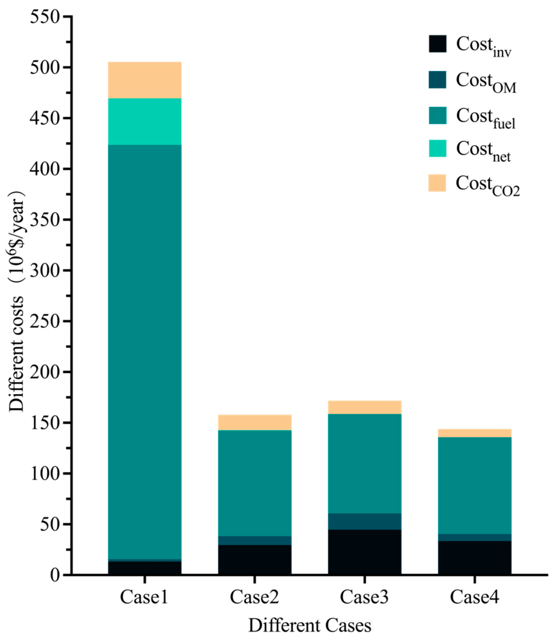
5.1. The Overall Results

This section presents and analyzes the key results of the four defined cases, focusing on installed capacities, total costs and their breakdowns, carbon emissions, and renewable energy performance metrics. Comparative performance across cases highlights strategies for achieving low-carbon and sustainable energy transitions in oilfield operations. Table 6 summarizes installed capacities, Figure 4 outlines cost distributions, and Table 7 demonstrates carbon emission reductions achieved through increased renewable energy integration and reduced reliance on fossil fuels.
Case 1 represents the baseline configuration, where gas turbines and natural gas boilers dominate the energy supply, ensuring reliable operations. The total system cost in Case 1 is the highest among all cases, driven by significant expenditures on fuel and electricity purchases. Carbon emissions are also highest in this case, underscoring the environmental impact of fossil fuel dependency. This baseline demonstrates the pressing need for low-carbon technologies to address the dual challenges of economic inefficiency and environmental sustainability.
In Case 2, the system allows for the integration of renewable energy and storage technologies. While the optimal configuration does not include renewable energy deployment, thermal energy storage is utilized to enhance system performance. Gas absorption heat pumps replace a substantial portion of natural gas boilers from the baseline scenario (Case 1), achieving higher efficiency with lower costs and emissions. The total costs in Case 2 are reduced by 69.76% compared to Case 1, driven by substantial decreases in fuel, grid electricity, and carbon costs. Carbon emissions declined by 36.96%, primarily due to the improved efficiency of heat supply. This case demonstrates that under the current market mechanism with no upper limit on grid electricity procurement, relying on grid power remains more economically viable than implementing renewable energy technologies.
Case 3 builds on Case 2 by eliminating grid electricity access, requiring greater reliance on local renewable energy and flexible generation technologies. The deployment of photovoltaic and wind turbines, coupled with a higher gas turbine capacity, compensates for the absence of grid electricity. However, this transition led to a 9.27% increase in total system costs compared to Case 2, driven by significant rises in investment and operational costs. Despite the higher costs, carbon emissions are further reduced by 7.08% compared to Case 2, as renewable energy offsets a portion of fossil fuel use. To meet the increased flexibility demands in Case 3, gas turbine capacity is significantly expanded compared to Case 2, while thermal storage capacity remains unchanged, limiting the role of battery energy storage systems in managing variability. Gas turbines are essential in providing flexibility to manage renewable energy intermittency, outperforming battery energy storage systems.
The integration of electrified equipment in Case 4 significantly reduces carbon emissions, despite its lower renewable energy capacity. Compared to Case 3, Case 4 achieves a 2.64% reduction in emissions and a 16.72% decrease in total costs, making it the most cost-effective scenario, with an annualized cost of USD 143.67 million. Enhanced thermal energy storage further improves the system’s capacity to manage heating fluctuations, supporting the efficient operation of electrified heat technologies.
Overall, while Case 2 demonstrates the cost-effectiveness of moderate reliance on the power grid under current conditions, Case 3 illustrates the trade-offs associated with achieving grid independence. Case 4 underscores the critical role of electrified heat in reducing carbon emissions. The progressive reduction in costs and emissions across the cases highlights the synergistic benefits of renewable energy integration, electrification, and optimized system configurations.

5.2. Sensitivity Analysis

5.2.1. Impacts of the Upper Limit of Electricity Purchase

The sensitivity analysis of the electricity purchase upper limits provides critical insights into the transition from Case 2 (full grid availability) to Case 3 (mandatory grid independence). By examining a range of power purchase limits, this analysis explores the implications of progressively reducing grid access on the configuration and performance of oilfield energy systems. It highlights how different levels of grid dependence influence the adoption of different units, emphasizing their role in achieving balanced and resilient energy supply under restricted external power conditions. The sensitivity analysis considers power purchase limits ranging from 0 MW to 24 MW with 2 MW increments. This parameter range was determined through preliminary testing, beyond which system behavior showed negligible variations. The selected 2 MW step size provides optimal resolution to observe meaningful configuration changes while maintaining computational efficiency.
Figure 5 summarizes the optimal capacity configurations for different technologies under varying power purchase limits. The installed capacities of different technologies reflect clear trends as power purchase limits decrease. Gas turbine capacity remains constant at 192 MW until the power purchase limit reaches 0 MW, at which point the capacity increases to 240 MW. This increase ensures a stable and reliable power supply, compensating for the loss of external grid support. Simultaneously, as power purchase limits decrease, the installed capacities of renewable energy and battery storage gradually increase. This shift is driven by the economic advantages of locally sourced renewable energy and storage solutions, which offset the high fuel costs and carbon emissions associated with gas turbines. Despite their intermittency, renewables paired with storage provide a cost-effective alternative, particularly when grid power is restricted.
However, the installed capacities of heat supply equipment, such as gas absorption heat pumps and natural gas boilers, as well as thermal energy storage systems, remain unchanged. This stability is attributed to the independence of the heating system from the power system and the relatively steady heat demand, which is met by the highly efficient heat pump and boiler configurations.
The cost analysis of varying power purchase limits, as shown in Figure 6, reveals the economic implications of power purchase constraints. As the power purchase limit decreases, total costs increase by 9.27% from the case with no restrictions to the case with zero grid purchases. This increase is driven primarily by significant rises in investment and operational costs, which outweigh the modest reductions in carbon emissions, power purchase, and fuel costs. The need to expand local energy infrastructure, including additional gas turbines, renewable energy systems, and storage solutions, accounts for the higher capital investment.
These findings carry significant implications for the design and planning of oilfield energy systems. While limiting grid purchases can accelerate low-carbon transitions by promoting renewable energy and storage adoption, the associated economic costs highlight the importance of balanced strategies. A gradual transition that combines moderate grid purchases with increased renewable energy integration is a more cost-effective approach, allowing systems to leverage the reliability and cost advantages of grid power while steadily reducing carbon emissions. Additionally, the results emphasize the critical role of flexible resources such as gas turbines and energy storage in maintaining system stability under constrained grid conditions. Policymakers and planners should prioritize investments in flexible and efficient technologies to optimize the trade-off between economic feasibility and decarbonization goals.

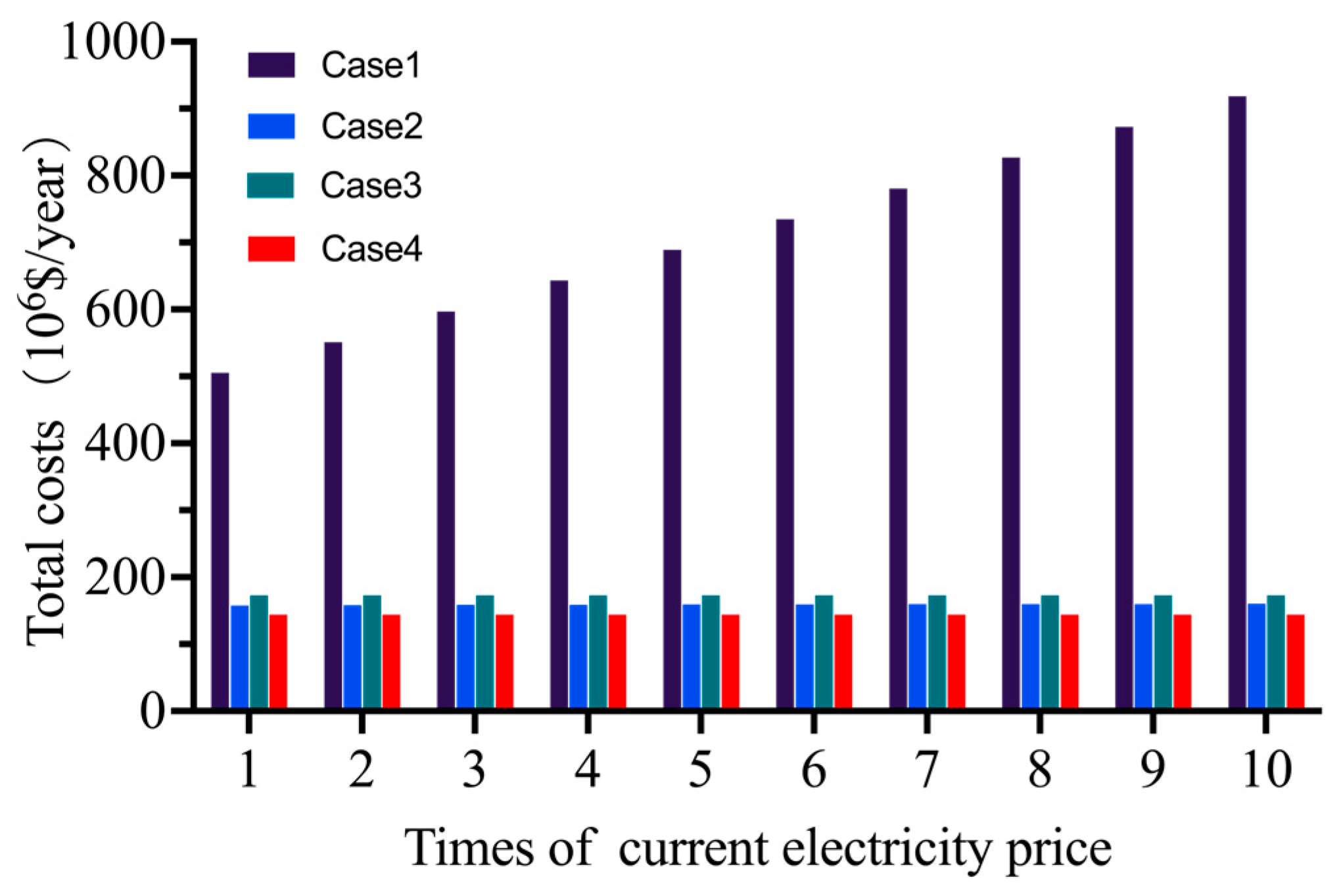
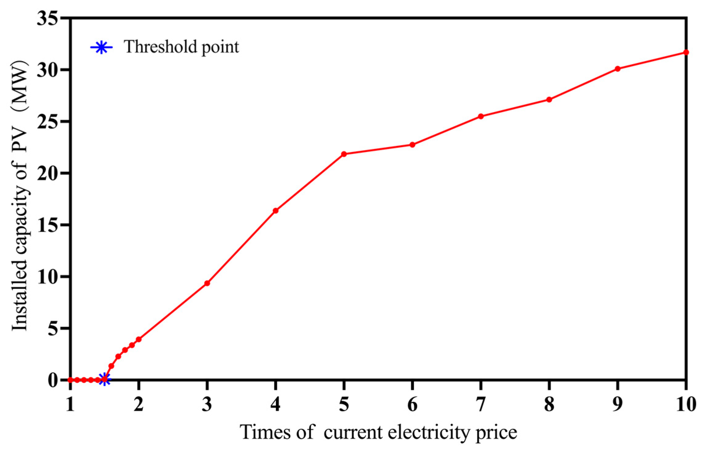
5.2.2. Impacts of Electrical Prices

As outlined in the Introduction Section, rising electricity prices can significantly affect operational costs and system design decisions. Our study evaluates how such price increases may impact the economic viability and operational strategies of oilfield energy systems. Using the time-of-use electricity prices from Section 4.1 as a baseline, we conduct a sensitivity analysis with price multipliers ranging from 1× to 10×.
The analysis of electricity price sensitivity demonstrates its profound impact on the costs of oilfield energy systems under different cases, as is shown in Figure 7. In Case 1, which represents a conventional fossil fuel-dominated system heavily reliant on grid electricity, total costs increase significantly as electricity prices rise. When the electricity prices show a ten-fold increase, the total costs escalate by 81.74%, rising from USD 505.41 million/year to USD 918.55 million/year. This linear cost increase, evident in Figure 7, reflects Case 1’s direct dependence on grid electricity, where each price increment proportionally raises electricity purchase expenses due to the system’s lack of alternative generation or storage options. This stark increase underscores the economic vulnerability of this configuration to electricity price fluctuations. The primary driver of this cost surge is the sharp rise in electricity purchase costs, while investment, operational, and fuel costs remain unchanged.
In Case 2, photovoltaic capacity is the only element that changes within the installed configuration as electricity prices rise, as shown in Figure 8. Based on model calculations, the critical electricity price threshold for initiating PV deployment is identified at 1.5 times the baseline electricity price, marked as the “Threshold point” in Figure 8. At this point, a small initial PV capacity of approximately 0.09 MW is deployed. As electricity prices increase further, PV capacity expands significantly, reaching approximately 31.68 MW at tenfold electricity prices. This analysis highlights the electricity price threshold at which renewable energy becomes economically viable, driven by the rising costs of grid electricity.
Furthermore, compared to Case 1, Case 2 exhibits exceptional economic resilience. Even under extreme price scenarios, the total costs increased by only 1.5%, from USD 157.89 million/year to USD 160.26 million/year. Compared to Case 1 and 2, Case 3 and 4 exhibit complete immunity to electricity price changes, with total costs remaining constant across all price levels. This economic stability underscores the potential of microgrid systems to effectively eliminate electricity price risks. These findings highlight that systems incorporating renewable energy or achieving self-sufficiency not only enhance economic stability but also contribute to greater sustainability, making them a robust solution for mitigating market volatility and supporting long-term energy resilience.

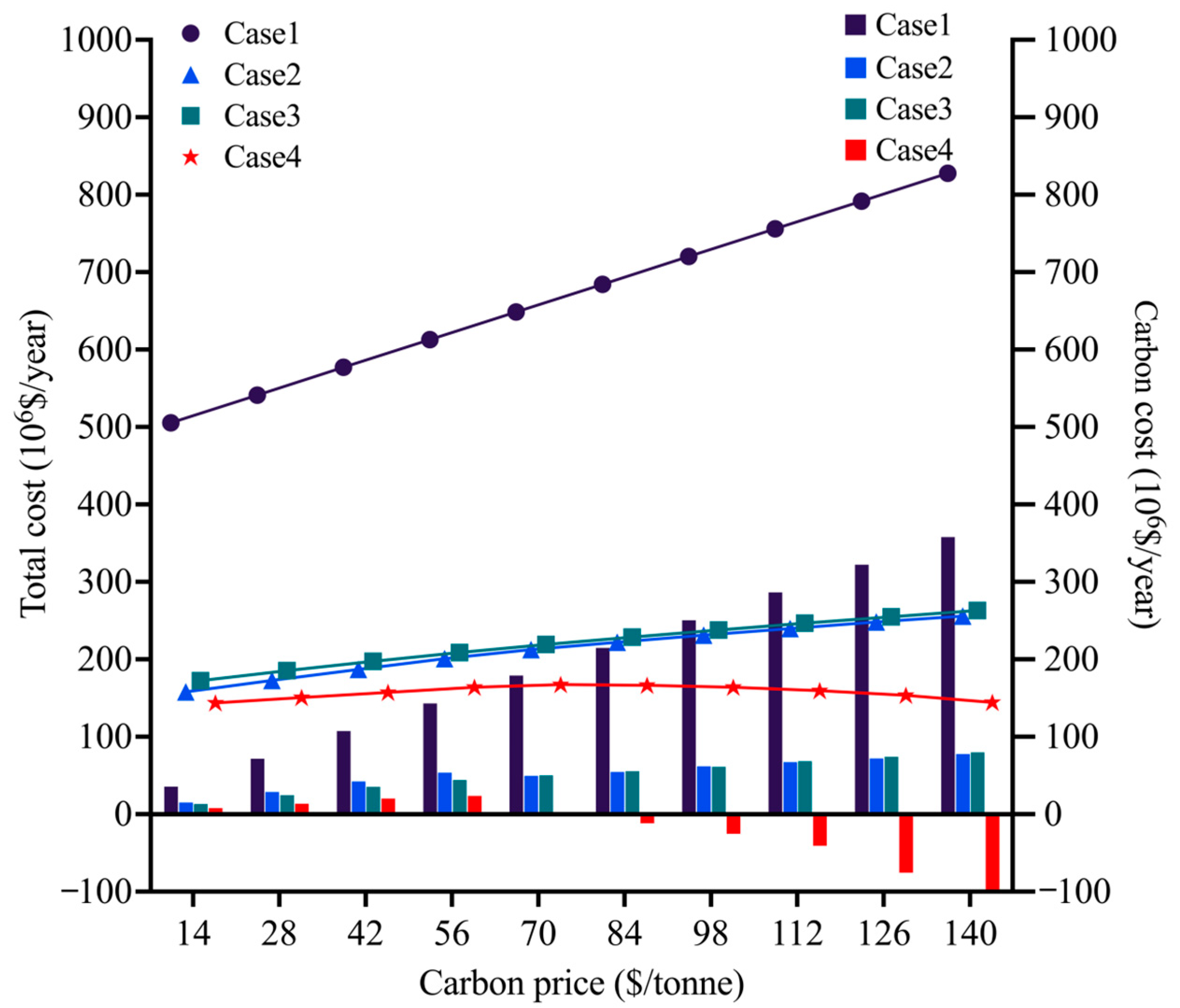
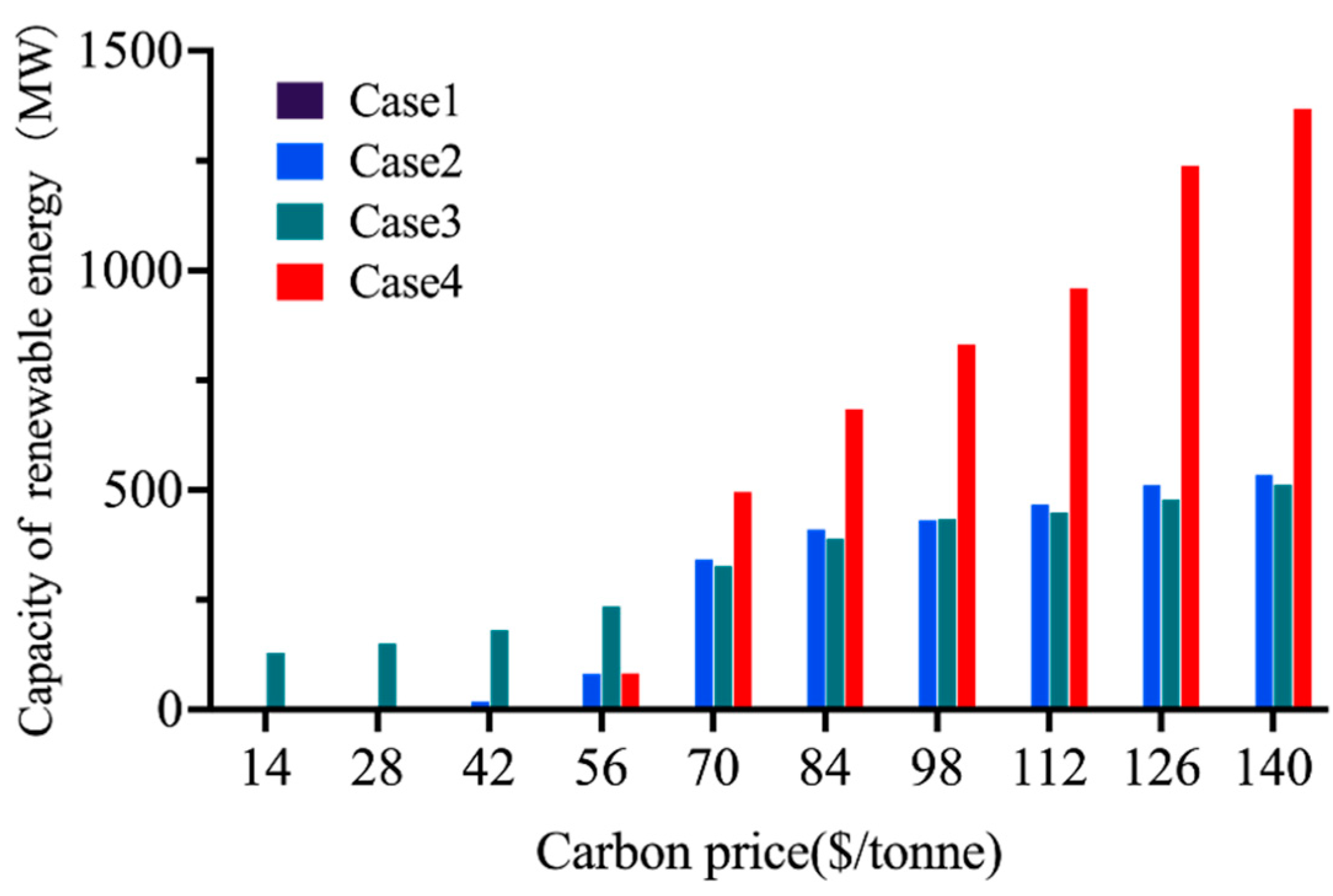
5.2.3. Impacts of Carbon Prices

Evaluating the impact of rising carbon prices on oilfield energy systems is crucial for assessing their economic resilience and adaptability under stricter carbon regulations. As previously noted, China’s national carbon market has experienced tightening emission allowances, resulting in a substantial rise in carbon prices. Therefore, this study conducts a sensitivity analysis to test the impact of rising carbon prices on system configuration and total costs. The carbon price is scaled from USD 14/tonne (the current carbon price in China [3]), to USD 140/tonne, representing a tenfold increase to simulate potential future scenarios influenced by evolving policies and market dynamics. This upper limit is consistent with the International Energy Agency’s (IEA’s) forecast, which estimates that under scenarios aligned with the Paris Agreement goals, carbon prices may reach USD 125–140/tonne by 2040 [38]. This analysis enables a comprehensive assessment of how rising carbon prices may affect the economic viability and strategic adjustments of oilfield energy systems under varying regulatory pressures.
The total cost variation across the cases varies significantly, as shown in Figure 9. The left panel displays the trend of annualized total costs under different carbon price scenarios through line charts, while the right panel highlights the corresponding annualized carbon emission costs through bar charts. From baseline carbon pricing (USD 14/tonne) to the highest carbon pricing scenario (USD 140/tonne), the annualized total costs increase by USD 322.16 million/year in Case 1, USD 98.10 million/year in Case 2, and USD 90.59 million/year in Case 3. The significant increase in costs for Case 1 is mainly attributed to its reliance on fossil fuel power generation, with carbon costs rising continuously as prices increase. Although its investment and operating costs remain unchanged, the compound effect of fuel and carbon costs has a significant impact on its overall cost structure, highlighting its vulnerability to strict carbon pricing. In contrast, the cost increases for Cases 2 and 3 are mitigated as the deployment of renewable energy increases.
Meanwhile, Case 4 shows a unique pattern, where the total cost initially rises with the increase in carbon prices but then falls, reaching a turning point at a carbon price of USD 76.4/tonne. At this threshold, the cost of carbon emissions in Case 4 shifts from positive to zero, as carbon emissions are within quotas due to the integration of widespread renewable energy and electrification. This turning point highlights the economic advantage of systems that actively reduce carbon emissions, ultimately benefiting from a carbon pricing mechanism aimed at penalizing high-emission configurations.
Figure 10 shows that under the higher carbon price scenario, Case 4 significantly increased the renewable energy capacity. The deployment of such photovoltaic systems and wind turbines offsets carbon costs, reduces dependence on fossil fuels, and enhances economic resilience under high carbon prices. Initial cost increases reflect investments in electrification and renewables, but as carbon prices exceed the turning point, low-operating-cost renewables lead to a net cost reduction. Overall, Case 4 exhibits the highest adaptability and economic robustness among the cases, highlighting the long-term viability of decarbonized energy systems in a carbon-neutral policy landscape.

6. Conclusions

This study developed a modeling and optimization framework to assess the integration of renewable energy into an oilfield energy system, focusing on balancing substantial heat and power demands with economic objectives. Through an optimization model with variable temporal resolution and an adaptive time-series aggregation algorithm, the framework evaluated four distinct cases for an oilfield in Northeast China. These cases explored baseline fossil fuel reliance, partial renewable integration with grid access, grid-independent microgrids, and heat electrification, analyzing their performance under varying electricity purchase limits, electricity prices, and carbon prices.
This study’s results reveal a progressive evolution in optimizing oilfield energy systems across four cases, balancing economic viability, energy stability, and decarbonization. In the baseline scenario (Case 1), reliance on gas turbines and natural gas boilers yielded high annualized total costs of USD 505.41 million/year, driven by fuel and grid electricity expenses. Introducing thermal energy storage and gas absorption heat pumps in Case 2 reduced costs by 69.76% to USD 157.89 million/year, demonstrating the immediate economic benefits of efficient heat supply technologies despite grid dependency. Case 3, a grid-independent microgrid, increased renewable capacity to 35% with a 192 MW gas turbine addition, raising costs by 9.27% over Case 2 due to investments in photovoltaic, wind, and storage systems, but ensuring operational resilience under constrained grid access. Case 4, incorporating electrified heat via electric heat pumps and boilers, achieved the lowest cost of USD 143.67 million/year and a 2.64% emissions reduction compared to Case 3, with renewable deployment becoming economically viable at 1.5 times the current electricity price and reaching a cost inflection point at a carbon price of USD 76.4 per tonne.
These findings highlight the transformative potential of strategic system design. Efficient technologies, as in Case 2, offer substantial cost savings, while grid-independent microgrids, as in Case 3, enhance resilience, particularly under rising electricity prices where independent systems show superior economic robustness. Case 4 incorporates electrified heating equipment, emphasizing the approach of combining cost-effectiveness with decarbonization. To support China’s carbon neutrality goal, the oil and gas industry should prioritize efficient electro thermalization equipment to minimize costs and emissions, and develop flexible microgrids to balance grid access with local renewable energy generation, ensuring economic and environmental sustainability.
Looking ahead, this work provides a hopeful outlook for advancing the study of the oilfield energy system. Future research can focus on long-term dynamic modeling to assess how evolving policy trends affect the optimization of the energy system over time. Additionally, exploring load transfer strategies for oil and gas pump stations may increase the use of renewable energy, potentially reduce reliance on gas turbines, and further lower costs. These advancements will enhance the adaptability and sustainability of oilfield operations, supporting broader carbon neutrality goals.
In conclusion, this study demonstrates that integrating efficient technologies, electrified heating, and renewable energy can significantly reduce costs and emissions in oilfield energy systems. By leveraging these strategies, the oil and gas industry can achieve economic resilience and environmental sustainability, contributing to global efforts toward a low-carbon future.

Author Contributions

Y.Z.: methodology, software, investigation, data curation, writing—original draft. J.L.: methodology, validation, investigation, project administration, writing—review and editing. P.L.: conceptualization, project administration, writing—review and editing. G.Z.: validation, funding acquisition. H.L.: supervision, funding acquisition. All authors have read and agreed to the published version of the manuscript.

Funding

This research was funded by Strategic Research and Consulting Project of Chinese Academy of Engineering (2024-XZ-88), and The National Natural Science Foundation of China (72140005).

Data Availability Statement

The original contributions presented in this study are included in the article. Further inquiries can be directed to the corresponding author.

Conflicts of Interest

Authors Jinze Li, Guosheng Zhang and He Liu were employed by the Research Institute of Petroleum Exploration and Development. The remaining authors declare that the research was conducted in the absence of any commercial or financial relationships that could be construed as a potential conflict of interest.

References

  1. Esiri, A.E.; Babayeju, O.A.; Ekemezie, I.O.; Esiri, A.E.; Babayeju, O.A.; Ekemezie, I.O. Implementing sustainable practices in oil and gas operations to minimize environmental footprint. GSC Adv. Res. Rev. 2024, 19, 112–121. [Google Scholar] [CrossRef]
  2. Esiri, A.E.; Sofoluwe, O.O.; Ukato, A. Aligning oil and gas industry practices with sustainable development goals (SDGs). Int. J. Appl. Res. Soc. Sci. 2024, 6, 1215–1226. [Google Scholar] [CrossRef]
  3. China ETS carbON PRICE Trends by Instrument 2024. Statista. Available online: https://www.statista.com/statistics/1474955/carbon-prices-in-china-by-ets/ (accessed on 23 January 2025).
  4. Wang, K.; Lv, C. Global and China Carbon Market Review and Outlook (2025); Center for Energy and Environmental Policy Research, Beijing Institute of Technology: Beijing, China, 2025. [Google Scholar]
  5. Bartolini, A.; Mazzoni, S.; Comodi, G.; Romagnoli, A. Impact of carbon pricing on distributed energy systems planning. Appl. Energy 2021, 301, 117324. [Google Scholar] [CrossRef]
  6. Schuldt, H.; Lessmann, K. Financing the low-carbon transition: The impact of financial frictions on clean investment. Macroecon. Dyn. 2021, 27, 1932–1971. [Google Scholar] [CrossRef]
  7. Boon, M. A Climate of Change? The Oil Industry and Decarbonization in Historical Perspective. Bus. Hist. Rev. 2019, 93, 101–125. [Google Scholar] [CrossRef]
  8. Guo, Y.; Yang, Y.; Bradshaw, M.; Wang, C.; Blondeel, M. Globalization and decarbonization: Changing strategies of global oil and gas companies. Wiley Interdiscip. Rev. Clim. Change 2023, 14, e849. [Google Scholar] [CrossRef]
  9. Morenov, V.; Leusheva, E.; Buslaev, G.; Gudmestad, O.T. System of Comprehensive Energy-Efficient Utilization of Associated Petroleum Gas with Reduced Carbon Footprint in the Field Conditions. Energies 2020, 13, 4921. [Google Scholar] [CrossRef]
  10. Veldhuis, A.J.; Leach, M.; Yang, A. The impact of increased decentralised generation on the reliability of an existing electricity network. Appl. Energy 2018, 215, 479–502. [Google Scholar] [CrossRef]
  11. IER Power Prices Spike in Norway. IER. 2024. Available online: https://www.instituteforenergyresearch.org/regulation/power-prices-spike-in-norway/ (accessed on 11 April 2025).
  12. Rai, A.; Nunn, O. On the impact of increasing penetration of variable renewables on electricity spot price extremes in Australia. Econ. Anal. Policy 2020, 67, 67–86. [Google Scholar] [CrossRef]
  13. Heptonstall, P.J.; Gross, R.J.K. A systematic review of the costs and impacts of integrating variable renewables into power grids. Nat. Energy 2021, 6, 72–83. [Google Scholar] [CrossRef]
  14. Bulut, M.; Özcan, E. Integration of Battery Energy Storage Systems into Natural Gas Combined Cycle Power Plants in Fuzzy Environment. J. Energy Storage 2021, 36, 102376. [Google Scholar] [CrossRef]
  15. Su, C.; Zhu, J.; Ma, J.; Xu, Y.; Zhao, Y. Thinking and suggestions on integrated development pathways for oil and gas with new energy. Pet. Sci. Technol. Forum 2024, 43, 18. [Google Scholar] [CrossRef]
  16. Huang, Y.; Zhao, W. Thoughts on promoting the integrated development of natural gas and renewable energy in China. World Pet. Ind. 2021, 28, 38–43. [Google Scholar]
  17. Abraham-Dukuma, M.C.; Dioha, M.O.; Aholu, O.C.; Emodi, N.V.; Ogbumgbada, C. A marriage of convenience or necessity? Research and policy implications for electrifying upstream petroleum production systems with renewables. Energy Res. Soc. Sci. 2021, 80, 102226. [Google Scholar] [CrossRef]
  18. Xiong, X.; Yun, Q.; Li, B.; Zhu, J. Thinking of clean replacement and re-electrification path for oil and gas production system under carbon peak and carbon neutrality goals. Pet. Sci. Technol. Forum 2023, 42, 21–29. [Google Scholar]
  19. Ozowe, W.; Ikevuje, A.H.; Ogbu, A.D.; Esiri, A.E. Renewable energy integration in offshore oil and gas installations. Magna Sci. Adv. Res. Rev. 2023, 8, 238–250. [Google Scholar] [CrossRef]
  20. Ekechukwu, D.E.; Simpa, P. Trends, insights, and future prospects of renewable energy integration within the oil and gas sector operations. World J. Adv. Eng. Technol. Sci. 2024, 12, 152–167. [Google Scholar] [CrossRef]
  21. Rafiee, A.; Khalilpour, K.R. Chapter 11—Renewable Hybridization of Oil and Gas Supply Chains. In Polygeneration with Polystorage for Chemical and Energy Hubs; Khalilpour, K.R., Ed.; Academic Press: Cambridge, MA, USA, 2019; pp. 331–372. ISBN 978-0-12-813306-4. [Google Scholar]
  22. Zhong, M.; Bazilian, M.D. Contours of the energy transition: Investment by international oil and gas companies in renewable energy. Electr. J. 2018, 31, 82–91. [Google Scholar] [CrossRef]
  23. Hartmann, J.; Inkpen, A.C.; Ramaswamy, K. Different shades of green: Global oil and gas companies and renewable energy. J. Int. Bus. Stud. 2021, 52, 879–903. [Google Scholar] [CrossRef]
  24. Choi, Y.; Lee, C.; Song, J. Review of Renewable Energy Technologies Utilized in the Oil and Gas Industry. Int. J. Renew. Energy Res. IJRER 2017, 7, 592–598. [Google Scholar]
  25. World Energy Outlook 2017; International Energy Agency (IEA): Paris, France, 2017.
  26. Electricity Storage and Renewables: Costs and Markets to 2030; International Renewable Energy Agency (IRENA): Masdar City, Abu Dhabi, 2017.
  27. Zhou, Z.; Liu, P.; Li, Z.; Ni, W. An engineering approach to the optimal design of distributed energy systems in China. Appl. Therm. Eng. 2013, 53, 387–396. [Google Scholar] [CrossRef]
  28. Qin, Y.; Liu, P.; Li, Z. Enhancing accuracy of flexibility characterization in integrated energy system design: A variable temporal resolution optimization method. Energy 2024, 288, 129804. [Google Scholar] [CrossRef]
  29. Murillo-Soto, L.D.; Meza, C. A Simple Temperature and Irradiance-Dependent Expression for the Efficiency of Photovoltaic Cells and Modules. In Proceedings of the 2018 IEEE 38th Central America and Panama Convention (CONCAPAN XXXVIII), San Salvador, El Salvador, 7–9 November 2018; pp. 1–6. Available online: https://ieeexplore.ieee.org/abstract/document/8596458?utm_source=chatgpt.com (accessed on 24 January 2025).
  30. Saint-Drenan, Y.-M.; Besseau, R.; Jansen, M.; Staffell, I.; Troccoli, A.; Dubus, L.; Schmidt, J.; Gruber, K.; Simões, S.G.; Heier, S. A parametric model for wind turbine power curves incorporating environmental conditions. Renew. Energy 2020, 157, 754–768. [Google Scholar] [CrossRef]
  31. Huang, Q.; Song, Y.; Sun, Q.; Ren, X.; Wang, W. Integrating Compressed CO2 Energy Storage in an Integrated Energy System. Energies 2024, 17, 1570. [Google Scholar] [CrossRef]
  32. Dou, X.; Wang, J.; Zhang, Z.; Gao, M. Optimal Configuration of Multitype Energy Storage for Integrated Energy Systems Considering System Reserve Value. CSEE J. Power Energy Syst. 2024, 10, 2114–2126. [Google Scholar] [CrossRef]
  33. Schittekatte, T.; Stadler, M.; Cardoso, G.; Mashayekh, S.; Sankar, N. The Impact of Short-Term Stochastic Variability in Solar Irradiance on Optimal Microgrid Design. IEEE Trans. Smart Grid 2018, 9, 1647–1656. [Google Scholar] [CrossRef]
  34. Cheng, Y.; Zhang, N.; Kirschen, D.S.; Huang, W.; Kang, C. Planning multiple energy systems for low-carbon districts with high penetration of renewable energy: An empirical study in China. Appl. Energy 2020, 261, 114390. [Google Scholar] [CrossRef]
  35. Renewable Power Generation Costs in 2023; International Renewable Energy Agency (IRENA): Masdar City, Abu Dhabi, 2024.
  36. Mongird, K.; Viswanathan, V.; Balducci, P.; Alam, J.; Fotedar, V.; Koritarov, V.; Hadjerioua, B. An Evaluation of Energy Storage Cost and Performance Characteristics. Energies 2020, 13, 3307. [Google Scholar] [CrossRef]
  37. Meteonorm Global Meteorological Database Version 8.2. Software and Data for Engineers, Planers and Education. Available online: https://meteonorm.com/assets/downloads/mn82_software.pdf (accessed on 1 April 2025).
  38. The Importance of Real-World Policy Packages to Drive Energy Transitions—Analysis. Available online: https://www.iea.org/commentaries/the-importance-of-real-world-policy-packages-to-drive-energy-transitions (accessed on 11 April 2025).
Figure 1. System structure diagram of renewable-integrated oilfield energy system.
Processes 13 01512 g001
Figure 2. Overview of power load and renewable energy power generation.
Processes 13 01512 g002
Figure 3. Comparison of original and aggregated data for representative days.
Processes 13 01512 g003
Figure 4. Breakdown of different cost components across four cases.
Processes 13 01512 g004
Figure 5. Optimal capacity configuration under varying power purchase limits.
Processes 13 01512 g005
Figure 6. Breakdown of different cost components under varying power purchase limits.
Processes 13 01512 g006
Figure 7. Sensitivity of total costs to increasing electricity prices.
Processes 13 01512 g007
Figure 8. Variation in PV capacity with increasing electricity prices in Case 2.
Processes 13 01512 g008
Figure 9. Total costs and carbon costs under varying carbon prices.
Processes 13 01512 g009
Figure 10. Optimal capacity configuration of renewable energy across difference cases.
Processes 13 01512 g010
Table 1. Technical parameters of the energy technologies.
TechnologyPrated (MW)Pmin (Prated%)ηrampmax (Prated%/min)Tschedule (min)
Gas turbine [28]4880%0.45%5
Photovoltaic system [28]-10%--1
Wind turbine [28]-10%--1
Electric boiler [34]520%0.95%1
Natural gas boiler [34]1030%0.85%10
Electric heat pump [34]1010%310%1
Gas absorption heat pump [34]415%1.310%5
Battery energy storage system [34]-0%0.92-1
Thermal energy storage system [34]-0%0.95-15
Table 2. Economic parameters of the energy technologies.
TechnologyPriceinv
(105USD/MW)
PriceOM,fid
(103 USD/MW/year)
PriceOM,var
(USD/(MW·h))
Lifespan
(y)
Maximum Capacity
(MW)
Gas turbine [28]4.125 5.111 2.013 30-
Photovoltaic system [35]6.710 3.800 0.000 201500
Wind turbine [35]9.860 23.009 0.000 201500
Electric boiler [34]1.528 1.911 0.000 20-
Natural gas boiler [34]2.083 1.389 1.875 20-
Electric heat pump [34]5.278 2.453 0.000 20-
Gas absorption heat pump [34]6.250 2.778 2.344 20-
Battery energy storage system [36]7.560 32.000 0.000 1510,000
Thermal energy storage system [34]0.500 0.017 0.000 2010,000
Table 3. Time-of-use electricity prices.
TimeElectricity Price (USD/kWh)
5:30–7:000.088
7:00–8:000.125
8:00–9:000.088
9:00–11:300.125
11:30–12:000.088
12:00–14:000.046
14:00–15:300.088
15:30–20:000.125
20:00–23:300.088
23:30–5:300.046
Table 4. Data compression performance for six representative days.
Day 1Day 2Day 3Day 4Day 5Day 6
Original data points144014401440144014401440
Aggregated data points 202230227300317236
Compression ratio 0.1400.1600.1580.2080.2200.164
Root mean squared error0.9590.9421.0810.9300.9340.955
Table 5. Key technology configurations across different cases.
Case 1 Case 2Case 3 Case 4
Gas turbine
Photovoltaic system×
Wind turbine×
Natural gas boiler
Electric boiler×××
Gas absorption heat pump
Electric heat pump×××
Battery energy storage system×
Thermal energy storage system×
Electricity purchase from the grid××
Table 6. Optimal capacity configurations of different technologies across four cases.
TechnologyThe Optimal Capacity (MW)
Case 1Case 2Case 3Case 4
Gas turbine96 192240288
Photovoltaic system00562
Wind turbine00740
Electric boiler00015
Natural gas boiler360909060
Electric heat pump000290
Gas absorption heat pump1227627624
Battery energy storage system0020
Thermal energy storage system05353158
Table 7. Analysis of carbon emissions and renewable energy metrics across four cases.
Case 1Case 2Case 3Case 4
Daily Average Carbon Emissions (t)8518.385369.864989.924858.00
Renewable Energy Utilization Rate --0.930.97
Renewable Energy Capacity Share-0.000.350.01
Renewable Energy Generation Share -0.000.100.00
Disclaimer/Publisher’s Note: The statements, opinions and data contained in all publications are solely those of the individual author(s) and contributor(s) and not of MDPI and/or the editor(s). MDPI and/or the editor(s) disclaim responsibility for any injury to people or property resulting from any ideas, methods, instructions or products referred to in the content.

