A Hybrid Framework for Production Prediction in High-Water-Cut Oil Wells: Decomposition-Feature Enhancement-Integration

Abstract

The forecasting of high-water-cut oil well production faces challenges of strong nonlinearity and nonstationarity due to reservoir heterogeneity and multiscale dynamic characteristics. This study proposes a hybrid CEEMDAN-SR-BiLSTM framework based on a “decomposition-feature enhancement-integration” architecture. The framework employs Complete Ensemble Empirical Mode Decomposition with Adaptive Noise (CEEMDAN) to suppress mode mixing, reconstructs high-, medium-, and low-frequency subsequences using Hilbert-Huang Transform (HHT) combined with tercile thresholding, and finally achieves multiscale feature fusion prediction through a Bayesian-optimized bidirectional long short-term memory network (BiLSTM). Interpretability analysis based on SHapley Additive exPlanations (SHAP) values reveals the contribution degrees of parameters such as water injection volume and flowing pressure to different frequency components, establishing a mapping between production data features and physical mechanisms of oil well production. This mapping, integrated with physical mechanisms including wellbore transient flow, injection-production response lag, and reservoir pressure evolution, enables mechanistic interpretation of production phenomena and quantitative decoupling and prediction of multiscale dynamics. Experimental results show that the framework achieves a root-mean-square error (RMSE) of 3.75 in forecasting a high-water-cut well (water cut = 87.6%) in the Qaidam Basin, reducing errors by 26.0% and 50.0% compared to CEEMDAN-BiLSTM and BiLSTM models, respectively, with a coefficient of determination (R²) reaching 0.954.

1. Introduction

Against the backdrop of continuously growing global energy demand, the status of oil as a core energy source remains irreplaceable [1]. However, as the world’s major oilfields generally enter the high water-cut development stage, the accuracy of well production forecasting has become a key factor restricting the potential tapping of remaining oil and development efficiency [2]. The dynamic evolution of well production is essentially the result of multi-physical field coupling, mainly influenced by factors such as wellbore flow conditions, injection-production pressure conduction, and reservoir energy evolution. Specifically, in wellbore transient flow, flow pattern transitions of multiphase fluids (oil, gas, water) (such as the alternation between slug flow and bubbly flow) cause drastic fluctuations in bottom-hole flowing pressure, directly affecting the efficiency of oil and gas lifting [3]. During injection-production processes, fluid seepage delay and pressure diffusion effects lead to time-lag responses in the near-wellbore area, weakening the uniformity of the displacement front [4,5]. Non-equilibrium pressure evolution in reservoirs, through the reconstruction of seepage-displacement coupling relationships, exacerbates the preferential development of channeling pathways and reduces waterflood sweep efficiency [6,7]. These unique cross-scale dynamic coupling effects in high water-cut reservoirs further intensify the difficulty of production forecasting.

Current mainstream forecasting methods have significant limitations. Physical-driven models based on Darcy’s law (such as reservoir numerical simulation) can accurately characterize seepage mechanisms, but their high complexity with billions of computational grids makes them difficult to meet real-time application requirements [8]. Empirical models represented by Arps decline curves and waterflood characteristic curves rely on historical data fitting from specific production stages and cannot adapt to production abrupt changes caused by reservoir heterogeneity variations or adjustments in development strategies [9,10,11].

In recent years, deep learning models represented by long short-term memory networks (LSTM) and their variant bidirectional long short-term memory networks (BiLSTM) have significantly improved the prediction efficiency of complex time-series data through a data-driven paradigm [12,13,14]. However, the strong nonlinearity and nonstationarity of production sequences in high water-cut reservoirs pose challenges to the multi-scale feature capture capability of single models. Against this backdrop, empirical mode decomposition (EMD) and its improved algorithm—complete ensemble empirical mode decomposition with adaptive noise (CEEMDAN)—have demonstrated unique advantages [15]. Through adaptive time-frequency decomposition, these methods decompose the original signal into intrinsic mode functions (IMFs) with characteristic scales, effectively separating high-frequency, medium-frequency, and low-frequency signal components, and providing a decomposition framework for multi-scale mechanism analysis of nonstationary signals [16]. Researchers have integrated them with deep learning in fields such as weather [17,18], hydrology [19], and energy [20,21], significantly enhancing the modeling capability of complex systems, and they have also shown satisfactory results in the field of well production forecasting [22]. However, existing studies mostly analyze the influence of single factors in isolation, lacking a connection between data-driven feature extraction and the physical mechanisms of well production—i.e., decomposing nonstationary signals into components corresponding to different physical mechanisms (wellbore dynamics, near-wellbore dynamics, and far-reservoir dynamic conduction)—while enabling quantitative analysis of feature contributions at different scales.

This study proposes a CEEMDAN-SR-BiLSTM framework based on a “decomposition-feature enhancement-integration” architecture. Specifically, CEEMDAN is used to decompose production signals into frequency components. Multi-scale features are enhanced through Hilbert-Huang transform and quantile-based reconstruction, classifying intrinsic mode functions (IMFs) into high-frequency, medium-frequency, and low-frequency components. A Bayesian-optimized bidirectional LSTM (BiLSTM) algorithm is employed for ensemble prediction, which independently models each frequency component to leverage bidirectional temporal dependencies while avoiding noise interference in raw data. Additionally, SHapley additive explanations are used to quantify feature contributions, revealing that the decomposed high-, medium-, and low-frequency curves correspond to the physical characteristics of wellbore transient flow, injection-production response lag, and reservoir pressure trends, respectively.

2. Materials and Methods

2.1. Research Data and Experimental Materials

The research data in this study are derived from 30 oil wells in the high water-cut development stage (comprehensive water cut > 80%) in Mangya, Qaidam Basin, China, encompassing full-life-cycle production data from January 1997 to December 2024. The target reservoirs are medium-to-high permeability sandstone reservoirs with an average porosity of 18.5% and permeability of 65 × 10⁻³ μm², exhibiting strong heterogeneity and multi-scale dynamic coupling.

Data Composition and Variable Definitions

Sample Size: A total of 30 wells were included, yielding 5040 monthly records in aggregate. The target well (validation well) has a water cut of 87.6%, representing the high-liquid production and low-oil production stage in the late development period. Specific statistical details are presented in

Table 1. Statistical Values of Variables Used in This Study.

	Maximum Value	Minimum Value	Average Value	Standard Deviation	Coefficient of Variation	Kurtosis	Skewness
Monthly Oil Production (t/month)	137.0	7.2	63.4	19.1	0.3	0.1	0.1
Flowing pressure (MPa)	16.1	7.6	11.8	2.1	0.2	−1.2	0.0
Water injection volume (m3/month)	284.2	50.0	139.8	47.7	0.3	−0.6	0.5
Fluid Level (m)	889.4	314.4	605.2	127.7	0.2	−1.0	0.0
Stroke (times/min)	3.0	3.0	3.0	0.0	0.0	0.0	0.0
Pump Strokes (times/min)	6.0	6.0	6.0	0.0	0.0	0.0	0.0
Casing Pressure (MPa)	4.0	1.2	2.6	0.5	0.2	−0.5	0.0
Porosity (%)	25.6	19.5	22.9	1.6	0.1	−0.7	0.2
Permeability (10−3 μm2)	300.0	80.0	192.4	70.8	0.4	−1.1	0.1
Operating time (years)	30.0	10.0	24.2	3.2	0.1	0.0	−0.5
Gas-Oil Ratio (GOR, m3/t)	107.1	65.1	85.3	7.1	0.1	−0.6	0.1

.

Feature Variables: (1) Production dynamic parameters: surrounding water injection volume (m³/month), producing gas-oil ratio (m³/t), flowing pressure (MPa), dynamic fluid level (m), casing pressure (MPa), stroke length, stroke frequency; (2) Wellbore process parameters: pump diameter (mm), pump depth (m), production time (years); Reservoir physical property parameters: porosity (%), permeability (10⁻³ μm²), effective thickness (m). (4) Label Variable: Monthly oil production (t/month), serving as the target for model prediction.

2.2. Data Preprocessing and Feature Selection

During the data preprocessing and feature selection phase, data normalization is first performed: the selected features undergo min-max normalization using the formula:

$$X^{\prime } = {\displaystyle \frac{X-X_{min}}{X_{max} - X_{min}}}$$

(1)

$X^{\prime }$: Normalized data value. $X$: Original feature data point. $X_{min}$: Historical minimum value of the feature. $X_{max}$: Historical maximum value of the feature.

Next, the processed data are subjected to Pearson correlation coefficient and mutual information criterion to identify dominant factors governing oil production, followed by feature selection on the preprocessed samples. The combined Pearson correlation coefficient and mutual information criterion are implemented through the following mathematical expressions: For two random variables X and Y, Pearson Correlation Coefficient:

$$r_{XY}={\displaystyle \frac{{\displaystyle \sum _{i=1}^n}(x_i-\overline{x})(y_i-\overline{y})}{\sqrt{{\displaystyle \sum _{i=1}^n}{(x_i-\overline{x})}^2{\displaystyle \sum _{i=1}^n}{(y_i-\overline{y})}^2}}}$$

(2)

$n$ represents the sample size, $x_i$ and $y_i$ are the $i-th$ observations of variables $X$ and $Y$, $\overline{x}$ and $\overline{y}$ denote the sample means of $X$ and $Y$. The Pearson correlation coefficient $r_{XY}$ ranges between $\left[-1,1\right]$:$r_{XY}=1$ indicates perfect positive correlation; $r_{XY}=-1$ indicates perfect negative correlation; $r_{XY}=0$ indicates no linear correlation

Mutual Information Value:

$$I(X,Y)=\sum _{x\in X}\sum _{y\in Y}p(x,y)\log ({\displaystyle \frac{p(x,y)}{p(x)p(y)}})$$

(3)

where $I(X,Y)$ quantifies the dependency between random variables $X$ (feature) and $Y$ (oil production). Here: $p(x,y)$ represents the joint probability distribution of X and Y; $p(x)$ and $p(y)$ denote the marginal probability distributions of X and Y, respectively.

2.3. Framework Design of CEEMDAN-SR-BiLSTM

2.3.1. Complete Ensemble Empirical Mode Decomposition with Adaptive Noise (CEEMDAN)

Complete Ensemble Empirical Mode Decomposition with Adaptive Noise (CEEMDAN) is an advanced method derived from the Empirical Mode Decomposition (EMD) algorithm. EMD, proposed by Huang [23], effectively analyzes non-stationary signals by decomposing them into Intrinsic Mode Functions (IMFs) that reflect local characteristics. However, EMD suffers from noise sensitivity and mode mixing arti-facts. To mitigate these issues, Ensemble EMD (EEMD) was developed by Wu et al. [24], which reduces noise influence through ensemble averaging. Nevertheless, EEMD introduces new challenges such as computational complexity and over-smoothed IMFs. To address these limitations, Complete Ensemble Empirical Mode Decomposition with Adaptive Noise (CEEMDAN) [25] was introduced, which overcomes mode mixing while maintaining decomposition effectiveness by adding and progressively adjusting noise levels to the signal. This method decomposes oil well production time-series data into multiple IMF components and a residual component through the following computational steps:

First, the original oil well production time series is combined with a Gaussian white noise sequence, introducing controlled randomness to reveal subtle variations hidden within the raw data. This hybrid sequence is then analyzed using Empirical Mode Decomposition (EMD) to extract its first-order Intrinsic Mode Function (IMF) component. As the primary decomposed layer, the IMF typically encapsulates the most prominent or fundamental dynamic characteristics of the sequence, enabling deeper insights into production variability.

$$im{\overline{f}}_1(t)={\displaystyle \frac{{\displaystyle \sum _{i=1}^{\mathrm{n}}}im{f}_1^i(t)}{\mathrm{n}}}$$

(4)

$im{\overline{f}}_1(t)$ represents the average component of the first-order IMF component, $im{f}_1^i$ denotes the $i-th$ IMF component obtained after the first decomposition, and indicates the maximum number of times white noise is added.

Calculating the first—order decomposition residue:

$$x_1\left(t\right)=P\left(t\right)-im{\overline{f}}_1(t)$$

(5)

Introduce the Gaussian white noise sequence into the first—order residue $x_1\left(t\right)$ to generate a new decomposition sequence $x_1^{\prime }\left(t\right)$. Subsequently, this new sequence undergoes EMD decomposition to obtain the second—order IMF component:

This process is iteratively repeated—mixing the oil well production time series with Gaussian white noise, performing EMD decomposition, and extracting IMFs—until the remaining residual sequence exhibits a monotonic trend. At this stage, the oil well production time series is decomposed and represented as the sum of a series of IMFs and a monotonic residual, enabling detailed analysis of production composition and variability. The decomposition formula is:

$$\mathrm{P}(\mathrm{t})=\sum _{\mathrm{j}=1}^{\mathrm{m}}im{\overline{f}}_j(t)+x_{\mathrm{k}}\left(\mathrm{t}\right)$$

(6)

where $x_{\mathrm{k}}\left(\mathrm{t}\right)$ represents the final residue.

2.3.2. Signal Reconstruction Algorithm (SR)

The Signal Reconstruction (SR) algorithm is a crucial component of the CEEMDAN-SR-BiLSTM framework for oil well production prediction. After the CEEMDAN decomposes the oil well production time-series into multiple Intrinsic Mode Function (IMF) components and a residual component, the SR algorithm plays a key role in processing and analyzing these decomposed components.

The main steps are as follows: First, the signal undergoes CEEMDAN decomposition to obtain IMF components. Then, the Hilbert-Huang Transform (HHT) is employed to calculate the instantaneous frequency of each IMF component. Subsequently, the IMF components are divided into high-frequency, medium-frequency, and low-frequency groups using the three-quantile method. Finally, the signal is reconstructed.

The Hilbert-Huang Transform (HHT) [26] is a mathematical tool for converting a real-valued signal into an analytic signal. It multiplies the negative-frequency part of the Fourier transform of a real-valued signal by—1 to yield a complex signal. The real part of this complex signal is the original real-valued signal, while the imaginary part is the Hilbert transform of the real-valued signal. First, the Hilbert-Huang Transform (HHT) is applied to the Intrinsic Mode Functions (IMFs) and residue obtained from CEEMDAN decomposition to calculate the instantaneous frequency of each IMF. The mathematical definition is:

$$\begin{array}{l}{f}_{i }(t)= {\displaystyle \frac{1}{2\pi }}{\displaystyle \frac{d{\varphi }_i (t)}{dt}} \\ {\varphi }_i(t)=\arctan \left({\displaystyle \frac{H[IM{F}_i(t)]}{IM{F}_i(t)}}\right)\\ \overline{f_i}={\displaystyle \frac{1}{T}} {\int }_T^0 f_i (t)dt\end{array}$$

(7)

where $f_{i }(t)$ is the instantaneous frequency of the $i-th$ $IMF$ component; ${\varphi }_i(t)$ is the phase function of this $IMF$, $H[IM{F}_i(t)]$ is the Hilbert transform result of $IM{F}_i(t)$, and $IM{F}_i(t)$ is the $i-th$ intrinsic mode function component. Here, $\overline{f_i}$ is the average frequency of the $i-th$ $IMF$, and $T$ is the signal duration.

Next, three-quantile frequency band division is performed by computing the three–quantiles $Q_{33 }$ and $Q_{66}$ of the average instantaneous frequencies ${\left\{{\overline{f}}_i\right\}}_{i=1}^n$ of all IMF components. IMFs are classified into high -, medium -, and low-frequency groups according to

$$\begin{array}{l}{X}_{high} =0,X_{mid} =0,X_{low} =0\\ X_{high} ={\sum }_{\overline{f_{i }}>Q_{66} } IM{F}_i \\ X_{med} ={\sum }_{Q_{33} <\overline{f_{i }} \le Q_{66} }IM{F}_i \\ X_{low} ={\sum }_{\overline{f_{i }} \le Q_{33} } IM{F}_i + Residue\\ Q_{33 }=quantile(\overline{f_{ i}} ,0.33)\\ Q_{66} =quantile(\overline{f_{ i}} ,0.66)\end{array}$$

(8)

where $Q_{33 }$ represents the 0.33 quantile of the average frequency sequence, and $Q_{66}$ represents the 0.66 quantile, both of which are used to divide the high, medium, and low frequency bands. $X_{high}$, $X_{med}$, $X_{low}$ are the reconstructed signals in the high, medium, and low frequency bands, and Residue is the residual term.

Finally, reconstruction performance validation is conducted using the Normalized Mean Squared Error (NMSE):

$$\begin{array}{l}NMSE= {\displaystyle \frac{{\left|X_{rec} - X_{orig}\right|}^2}{{\left|X_{orig}\right|}^2}} \\ X_{\mathrm{rec}}=X_{\mathrm{high}}+X_{\mathrm{mid}}+X_{\mathrm{low}}\end{array}$$

(9)

where NMSE stands for the Normalized Mean Square Error, $X_{rec }$ is the reconstructed signal, and $X_{orig}$ is the original signal.

2.3.3. Bayesian Optimization of Bidirectional LSTM Network

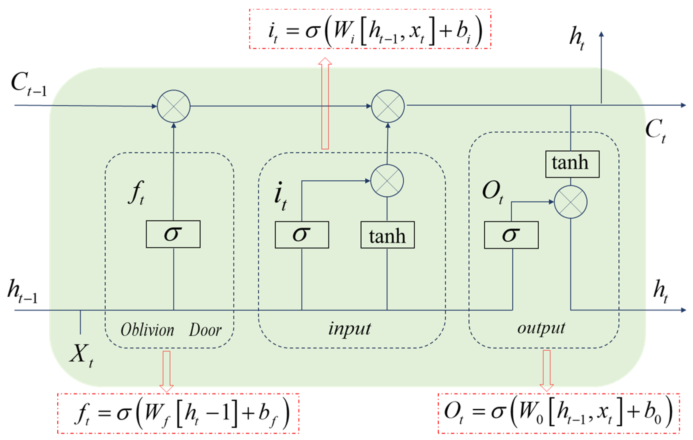
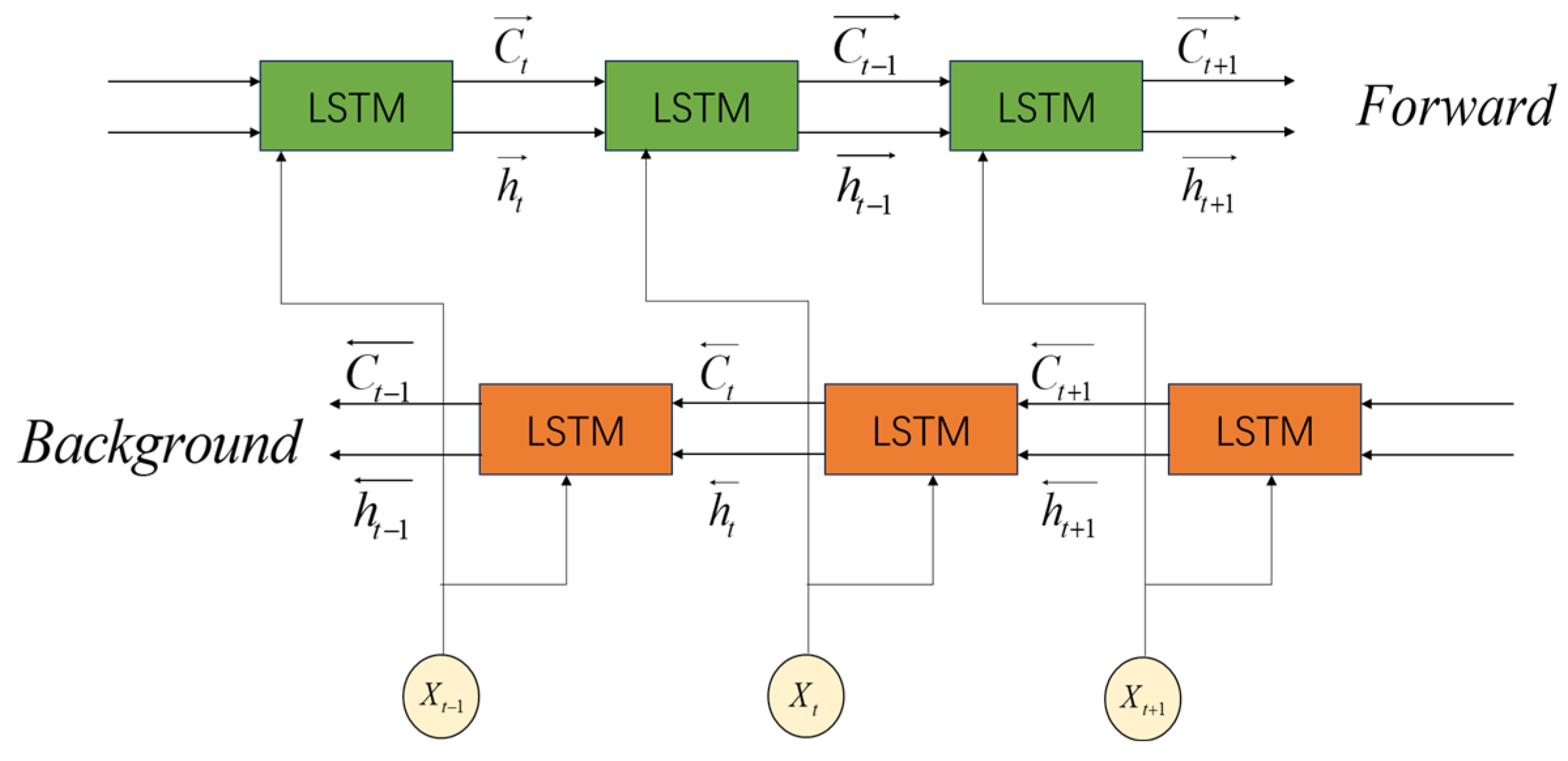
In recent years, deep neural networks represented by the Bidirectional Long Short-Term Memory (BiLSTM) network have achieved significant progress in multiple research fields. BiLSTM is an improved architecture based on the Long Short-Term Memory (LSTM) network [27] (as shown in Figure 1), characterized by its integration of forward and backward LSTM layers to form a bidirectional processing mechanism. In this architecture: The forward LSTM layer processes input sequences from left to right, capturing temporal dependencies in the forward direction. The backward LSTM layer processes sequences from right to left, uncovering backward dependencies in the data. This bidirectional processing mechanism enables BiLSTM to utilize both past and future information for prediction. Compared to traditional unidirectional LSTM, it comprehensively understands sequential data by capturing bidirectional contextual information, thereby significantly enhancing prediction performance (as shown in Figure 2).

The detailed computational process is as follows:

$$\begin{array}{l}{f}_t=\sigma (W_f\cdot [h_{t-1},x_t]+b_f)\\ i_t=\sigma (W_i\cdot [h_{t-1},x_t]+b_i)\\ O_t=\sigma \left(W_0\left[h_{t-1},x_t\right]+b_0\right)\end{array}$$

(10)

$x_t$ represents the input at time step t; $h_{t-1}$ denotes the hidden state at time step t − 1, serving as the output of the LSTM unit at the previous time step; $C_{t-1}$ indicates the cell state at time step t − 1, which is the state used for long-term memory within the LSTM unit. $\sigma$ stands for the sigmoid function; $W_f$, $W_i$, $W_0$ are the weight matrices of the forget gate, input gate, and output gate respectively; $b_f$, $b_i$, $b_0$ are the bias vectors of the forget gate, input gate, and output gate respectively.

$$\begin{array}{l}\overrightarrow{C_t}=LSTM(x_t,\overrightarrow{h_{t-1}},\overrightarrow{C_{t-1}})\\ \overleftarrow{C_t}=LSTM(x_t,\overleftarrow{h_{t-1}},\overleftarrow{C_{t-1}})\\ C_t=W^T\overleftarrow{C_t}+W^V\overleftarrow{C_t}\end{array}$$

(11)

$\overrightarrow{C_t}$ and $\overleftarrow{C_t}$ represent the cell states of the forward LSTM and backward LSTM at time step t. $W^T$ and $W^V$ denote the weight coefficients of the forward LSTM and backward LSTM.

To further enhance the prediction accuracy of the BiLSTM model, this study em-ploys Bayesian optimization to fine-tune the network’s hyperparameters. Bayesian optimization is an efficient global optimization algorithm that adaptively selects optimal hyperparameter combinations in each iteration based on surrogate model approximations of the actual objective function [28]. By leveraging a Gaussian process as the surrogate model and pairing it with the Expected Improvement (EI) acquisition function, this method identifies near—optimal hyperparameters within fewer iterations, making it particularly suitable for optimizing black—box objective functions with high evaluation costs. Consequently, Bayesian optimization has been widely ap-plied in hyperparameter tuning for machine learning and deep learning, significantly improving model performance (as shown in Figure 3).

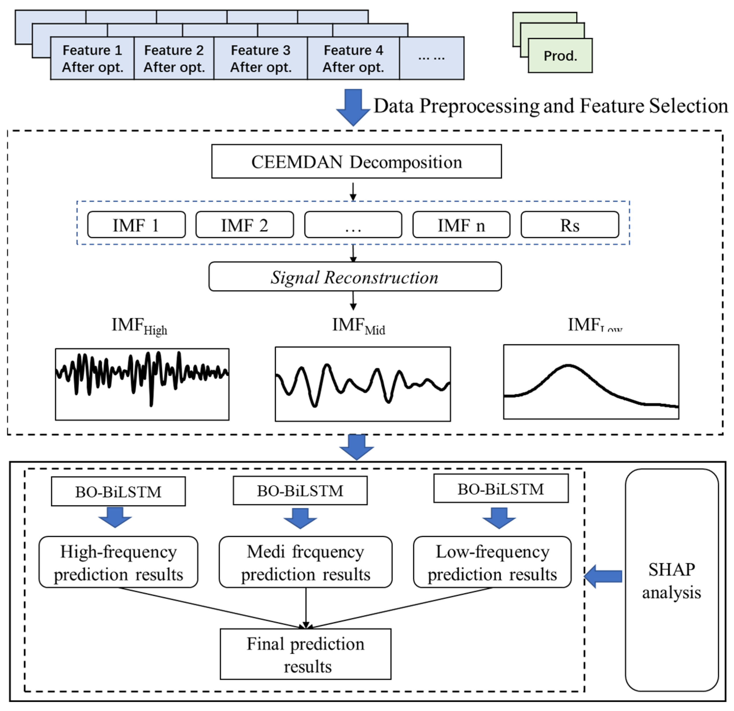
2.3.4. CEEMDAN-SR-BiLSTM

This section systematically describes the model application framework: First, data are preprocessed using the Pearson correlation coefficient-mutual information joint screening method to extract key features related to monthly oil production and eliminate redundant variables. Second, CEEMDAN is employed for multi-scale decomposition of production sequences. Combined with the Hilbert-Huang transform and tercile quantile threshold method, IMF components are reconstructed into high-frequency, medium-frequency, and low-frequency subsequences. Subsequently, a Bayesian-optimized BiLSTM model is used to model each subsequence, generating prediction results through linear combination. SHapley values are applied to quantify feature contributions, establishing associations between data features and reservoir physical mechanisms. Finally, comparative models are introduced to validate effectiveness. In the model architecture, CEEMDAN enables multi-scale signal decomposition, SR completes the physical meaning reconstruction of features, BiLSTM performs sequence prediction, forming an integrated production prediction model with mechanism analysis capabilities. SHapley values are used to quantify feature contributions and establish links between data features and reservoir physical mechanisms (as shown in Figure 4).

2.4. Model Evaluation Metrics

The criteria for evaluating model performance are the Mean Absolute Error (MAE), Root Mean Squared Error (RMSE), and the coefficient of determination ($R^2$), mathematically expressed as follows:

$$\begin{array}{l}RMSE=\sqrt{{\displaystyle \frac{1}{n}}{\displaystyle \sum _{i=1}^n}{(Q_i-Q_i^{\ast })}^2}\\ MAE={\displaystyle \frac{1}{n}}{\displaystyle \sum _{i=1}^n}\left|Q_i-Q_i^{\ast }\right|\\ R^2=1-{\displaystyle \frac{{\displaystyle \sum _{i=1}^n}{(Q_i-Q_i^{\ast })}^2}{{\displaystyle \sum _{i=1}^n}{(Q_i-\overline{Q})}^2}}\end{array}$$

(12)

Here, n represents the number of time series, $\overline{Q}$ is the average value of oil well production data, $Q_i$ is the true oil well production data value, and $Q_i^{\ast }$ is the predicted oil well production data value.

3. Results

This study focuses on a medium-to-high permeability sandstone reservoir in western China, where favorable hydrocarbon storage conditions exist but the field has entered a high water-cut development stage. Although crude oil production has remained relatively stable, both liquid production and average water cut have been increasing annually, presenting challenges for single-well production forecasting as development performance deteriorates. To address this issue, production data from 30 oil wells in the study area spanning 1997–2024 were collected. The dataset includes monthly records of 12 dimensions: surrounding water injection volume, producing gas-oil ratio, flowing pressure, pump diameter, pump depth, production time, porosity, permeability, casing pressure, dynamic fluid level, stroke count, and monthly oil production (with the latter serving as the labeled feature).

3.1. Data Preprocessing and Feature Selection

The comprehensive use of all indicators would obscure the validity of the data and significantly increase the computational load; therefore, irrelevant features were removed through screening to retain key parameters [29,30]. In this study, a feature selection method combining Pearson correlation coefficient analysis and p-value testing (α = 0.05) was employed [31]. Firstly, parameters with absolute Pearson correlation coefficients (|R|) greater than 0.35 were selected. The mutual information criterion (MI > 0.15) was introduced to cross-validate nonlinear associations. 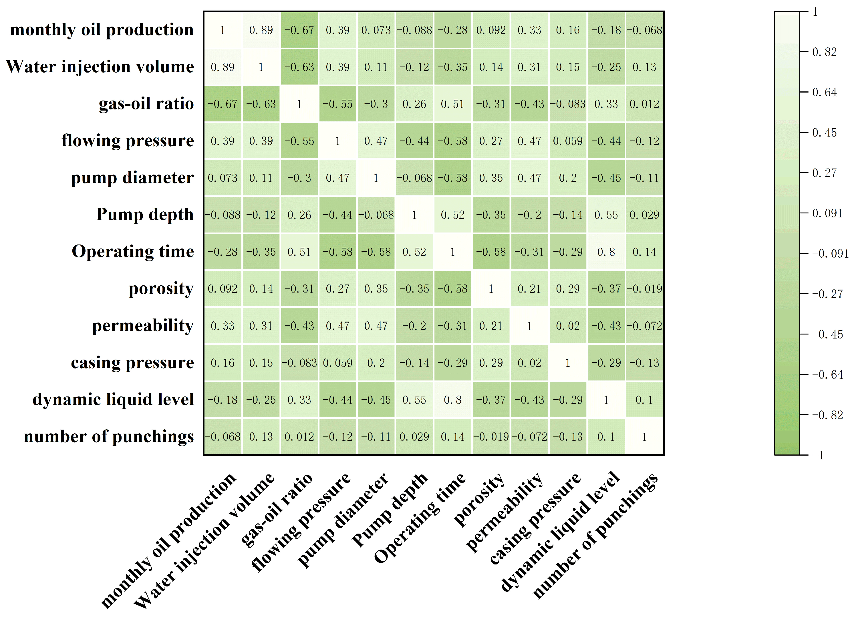The final key features determined via joint screening (p ≤ 0.05, |R| > 0.35, MI > 0.15) included water injection volume, gas-oil ratio, flowing pressure, operation time, and dynamic fluid level, reducing redundancy by 58.3%. Figure 5 presents the full correlation matrix from the Pearson correlation analysis, illustrating the pairwise correlation coefficients be-tween all feature parameters and monthly oil production, which helps identify significant linear relationships among variables.

Table 2. Mutual Information Values for Oil Production.

Feature	Mutual Information Value
Water injection volume	0.26
Gas-oil ratio	0.24
Flowing pressure	0.18
Pump diameter	0.122
Pump depth	0.033
Operating time	0.19
Porosity	0.189
Permeability	0.15
Casing pressure	0.042
Dynamic liquid level	0.175
Number of punchings	0.06

Note: Features with mutual information (MI) > 0.15 bits were selected for modeling, consistent with the nonlinear correlation screening criteria.

lists the mutual information values for oil production, quantifying the nonlinear associations between each feature and the target variable to assess their relevance in a non-parametric manner. Together, these two analyses form the basis for the feature screening process, enabling the selection of key indicators that significantly impact oil production while reducing dimensionality and computational complexity in subsequent modeling steps.

3.2. Multiscale Decomposition of Single-Well Oil Production

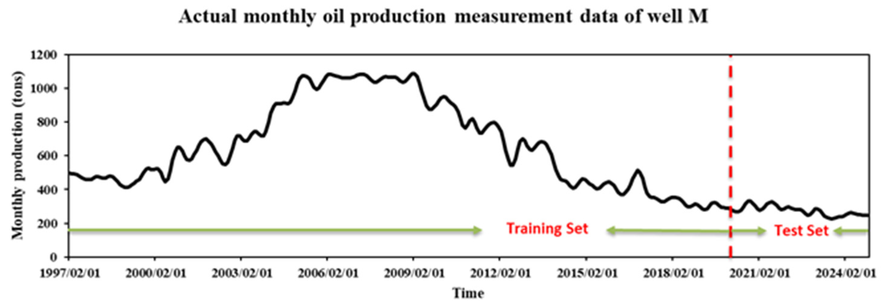
This study selected monthly oil production data from 1997–2024 for a high water-cut oil well (current water cut = 87.6%) in the target area. The original production curve exhibits a trend of initial fluctuating increase followed by fluctuating decline, with significant early-stage volatility and upward momentum, and reduced late-stage volatility leading to gradual decline. This reflects the well’s production lifecycle: production increase phase → stable phase → decline phase. The production data demonstrate strong nonlinearity and non-stationarity, characterized by significant temporal complexity. The training set included the first 90% of the dataset for model training, while the remaining 10% served as the test set for prediction evaluation. The time series plot of monthly oil production for this well is shown in Figure 6.

The CEEMDAN method effectively separates fluctuation features at different time scales from the original oil production signal. As shown in Figure 5, the data stream is decomposed into 4 Intrinsic Mode Functions (IMFs) and a residual component (IMF 5). The initial IMF components exhibit the highest volatility and frequency with the shortest wavelength, while subsequent components gradually weaken. The residual IMF 5 represents the long-term trend of the signal, showing an overall declining pattern. Default CEEMDAN parameters include: Gaussian white noise amplitude of 0.2, ensemble number of 500, and maximum iterations of 5000. The decomposition results are visualized in Figure 7.

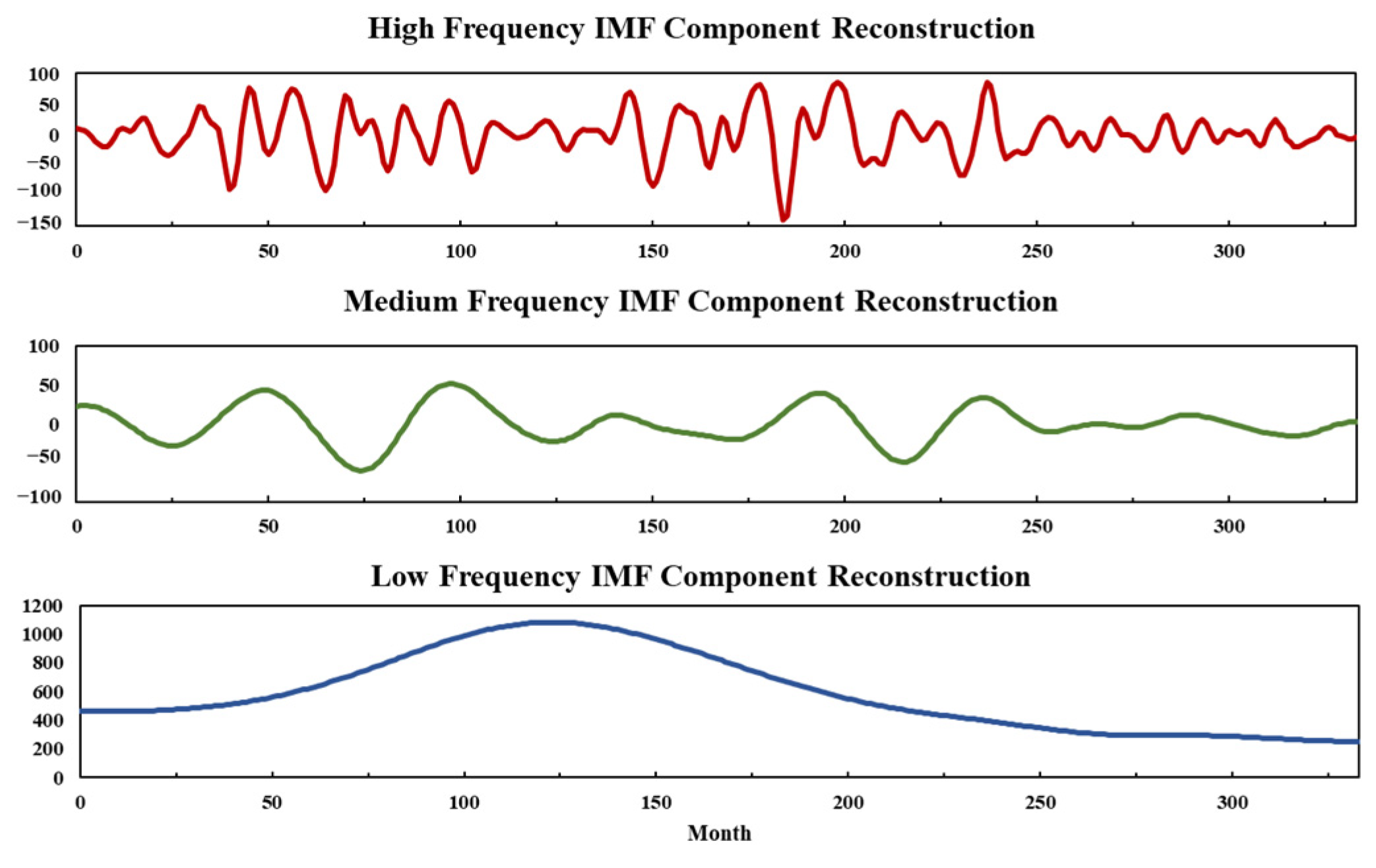
3.3. Signal Reconstruction and Multiscale Dynamic Feature Analysis

To achieve multiscale time-frequency characterization of signals, Hilbert transforms were first performed on CEEMDAN-decomposed IMF components to calculate mean instantaneous frequencies (MIF) for quantifying frequency properties (

Table 3. Mean Frequency Data of IMF Components.

IMF	Mean Frequency (Hz)	Frequency Band
IMF1	0.239658	High-frequency
IMF2	0.131594	High-frequency
IMF3	0.062700	Medium-frequency
IMF4	0.023700	Low-frequency
IMF5	−0.000165	Low-frequency (Residue)

). Using 33.33% and 66.66% quantiles of MIF as thresholds, IMFs were classified into three frequency bands: high-frequency (MIF > 66.66%), medium-frequency (33.33% < MIF ≤ 66.66%), and low-frequency (MIF ≤ 33.33% + residual term). Final band-specific signals were reconstructed via component summation strategy (Figure 8).

This study establishes a mapping between CEEMDAN-decomposed IMF components and multiscale dynamic features of oil well production via Physical Annotation [20], bridging data characteristics to physical mechanisms.

As shown in Figure 6: The high-frequency component exhibits frequent fluctuations with rapid amplitude changes, reflecting short-time-scale dynamics. The medium-frequency component features relatively smooth oscillations with periodicity longer than the high-frequency component, indicating mid-scale cyclic behavior. The low-frequency component demonstrates a clear trend of initial increase followed by decline, representing long-term evolutionary characteristics. From the perspective of Physical Mechanism of Oil Well Production, this correspondence between frequency and dynamic features is inherently deterministic.

High-frequency component: Corresponds to wellbore transient flow. As the direct channel for hydrocarbon production, the wellbore experiences rapid transient processes like throttling effects and fluid slippage phenomena. For example, sudden changes in fluid velocity and gas-liquid slippage during production generate high-frequency signals, making the high-frequency component the natural carrier of wellbore transient flow dynamics.

Medium-frequency component: Reflects injection-production response lag. In injection-production systems, reservoir seepage resistance and capillary forces act over mid-scale timeframes rather than instantaneously. When fluids are injected or produced, reservoir fluids require time to overcome seepage resistance and flow toward the wellbore, while capillary forces influence two-phase flow dynamics. These mid-scale processes—neither as rapid as wellbore transients nor as slow as reservoir pressure trends—are effectively characterized by the medium-frequency component, capturing both response lags and mid-scale seepage behavior.

Low-frequency component: Represents reservoir pressure trends. Reservoir pressure changes are long-term cumulative effects, including energy depletion (e.g., sustained pressure decline under natural drive) and waterflood recharge. The low-frequency component, combined with the residual term, precisely captures these gradual trends due to its frequency matching the “slow-varying” time scale of reservoir pressure, serving as an effective carrier for extracting long-term reservoir dynamics.

This frequency-physics mapping inherently correlates signal processing results with the time scales and operational characteristics of oil production processes, providing an analytical bridge between “signal frequency” and “physical processes” for multiscale dynamic analysis from the wellbore to near-wellbore zones and distant reservoirs.

3.4. Model Parameter Optimization Strategy

This study constructs a hierarchical parameter optimization framework, implementing differentiated strategies tailored to the characteristics of different frequency band signals (

Table 4. Optimal Hyperparameter Combinations for High-, Medium-, and Low-Frequency BiLSTM Models.

Parameter	High-Frequency	Medium-Frequency	Low-Frequency
hidden_size	92	117	82
num_layers	3	1	1
dropout	0.182	0.381	0.0912
learning_rate	0.001	0.001	0.001
hidden_size	92	117	82

Note: Parameters optimized via Bayesian optimization with Gaussian process model for high-frequency components, and manual tuning for medium- and low-frequency components based on signal periodicity and trend characteristics.

):

3.4.1. High-Frequency Component Optimization (BiLSTM)

Global parameter search via Bayesian optimization algorithm, dynamically balancing exploration and exploitation in the parameter space using a Gaussian process model. Optimization focused on network capacity and training stability yielded the optimal parameters: Hidden layer size: 92; Number of layers: 3; Dropout rate: 0.182; Learning rate: 0.001 (Adam optimizer with adaptive learning rate strategy).

3.4.2. Medium-Frequency Component Optimization (BiLSTM)

Given the significant periodicity of medium-frequency signals, strategies emphasized adjusting network depth and regularization parameters: Hidden layer size: 117; Number of layers: 1; Dropout rate: 0.381; Learning rate: 0.001.

3.4.3. Low-Frequency Component Optimization (BiLSTM)

To capture long-term trends, optimization prioritized overfitting suppression and trend-tracking enhancement: Hidden layer size: 82; Number of layers: 1; Dropout rate: 0.0912; Learning rate: 0.001.

3.5. Experimental Results

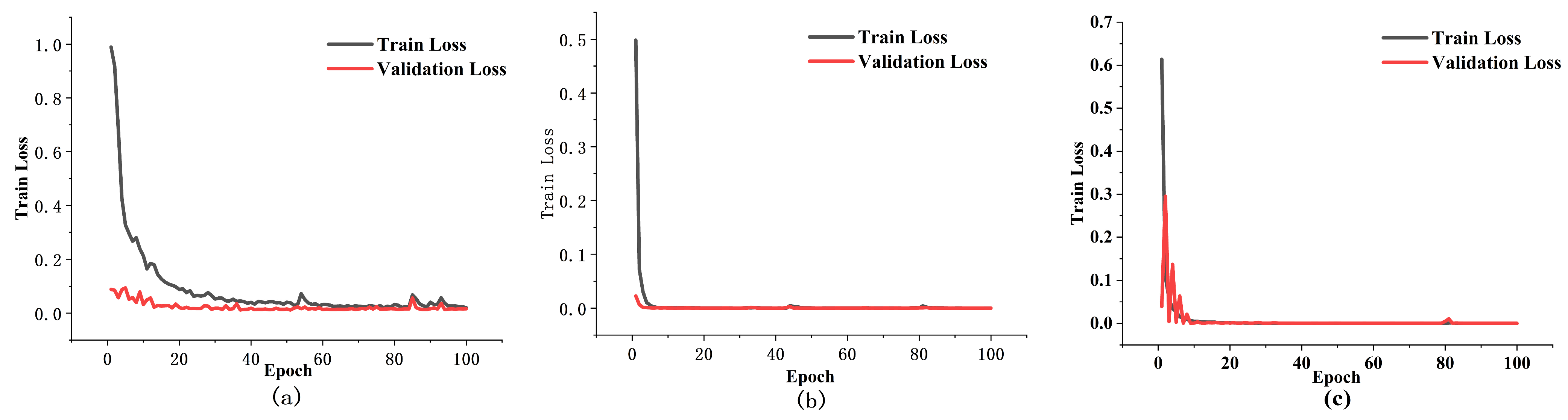
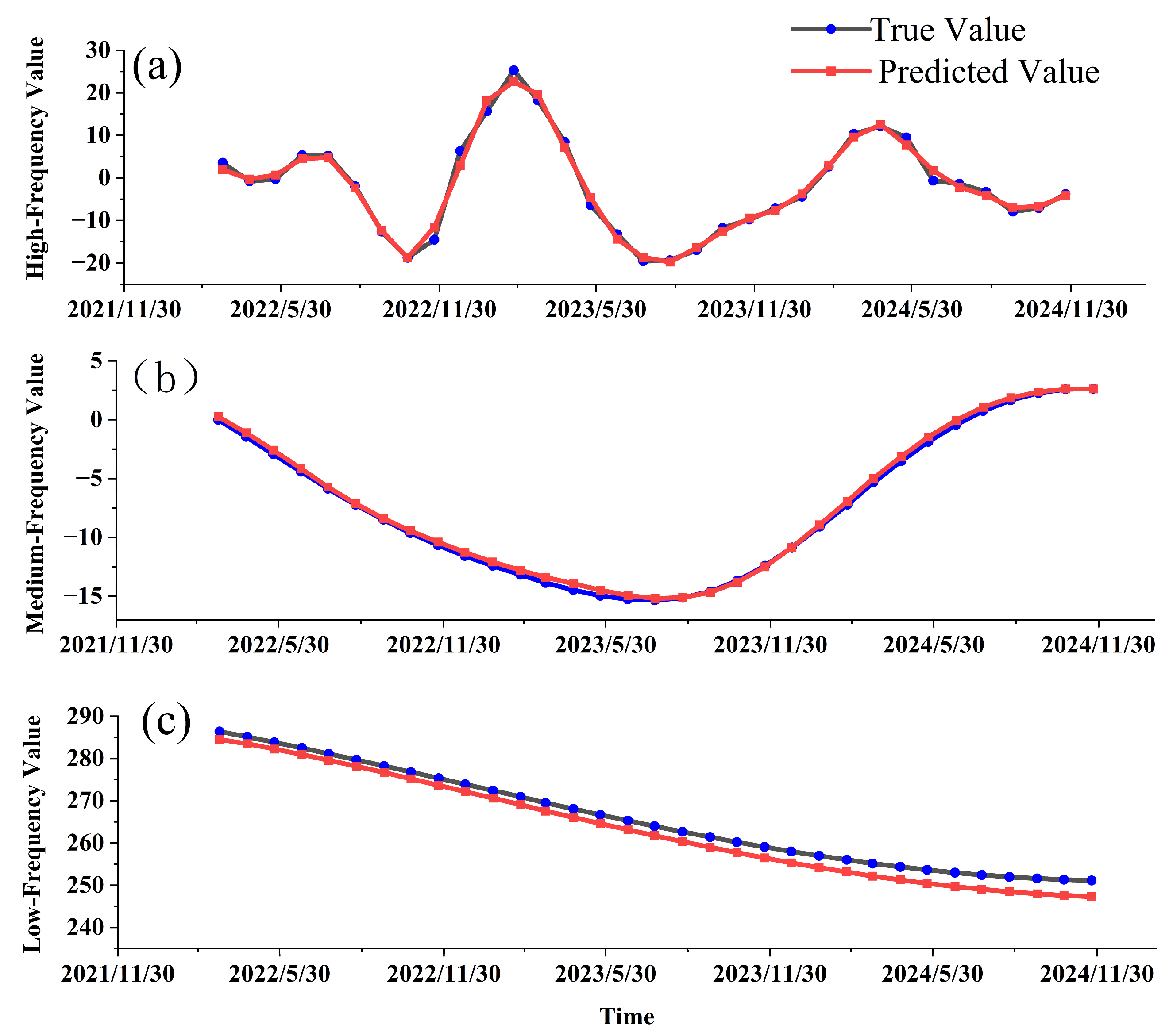
In this subsection, we conduct production forecasting using the CEEMDAN-SR-BiLSTM model. Given the relatively limited dataset size, the first 90% of the data was partitioned into the training set to ensure the model receives sufficient training, while the remaining 10% served as the test set. Figure 7 illustrates the training and test loss evolution during high-, medium-, and low-frequency predictions, and Figure 9 presents the corresponding forecasting results.

Figure 10a–c show differentiated convergence characteristics of training and validation loss curves for high-, medium-, and low-frequency component predictions: High-frequency: Training loss exponentially decreased from 3.2 to 0.8, with validation loss stabilizing in the range of 1.0 ± 0.2. Medium-frequency: Training loss converged to 0.3 within 20 iterations, with validation loss synchronously stabilizing at 0.4. Low-frequency: Training loss dropped by 78% (from 5.6 to 1.2) initially, with validation loss stabilizing at 1.5 after 30 iterations.

All three loss curves maintained a favorable state where training loss ≤ validation loss and synchronous convergence was achieved, validating the model’s effective capture capabilities for high/medium/low-frequency features and stability during training.

The CEEMDAN-SR-BiLSTM model demonstrates robust multiscale forecasting capabilities, accurately capturing dynamic trends across high-, medium-, and low-frequency components while maintaining overall prediction precision (RMSE = 3.75, MAE = 2.80, R² = 0.954). High-frequency predictions effectively track transient flow fluctuations (e.g., 2023 pump adjustment peaks) with RMSE = 1.89, though abrupt changes pose residual challenges. Medium-frequency results show improving alignment over time, achieving R² = 0.91 in late-stage injection-response cycles after initial bias reduction. Low-frequency trends align closely with reservoir pressure depletion (MAE = 1.23), with minor rate discrepancies highlighting geological heterogeneity impacts. The aggregated production forecast matches field measurements at critical inflection points (e.g., 2022Q1 ±1.5 t/month error) and stable periods (2022-11 to 2023-01 R² = 0.973), validating the model’s ability to synthesize multiscale physics-driven features for oil production analysis (

Table 5. CEEMDAN-SR-BiLSTM Multiscale Production Forecasting Evaluation Metrics.

Component	RMSE (t/Month)	MAE (t/Month)	R2
High-Frequency	1.3593	1.0608	0.9850
Medium-Frequency	0.2424	0.1949	0.9991
Low-Frequency	2.4520	2.3724	0.9780
Combined Total	3.7498	2.7966	0.9539

).

3.6. SHAP Values Theory for Production Fluctuation Interpretation and Physical Mechanism Characterization

To enhance the interpretability of the model, this study uses the SHAP tool (SHapley Additive exPlanations) to quantify the contribution of features in the prediction of production components [32]. This method is based on the Shapley value in cooperative game theory [33]. By regarding the model prediction as a ‘cooperative game’ of feature interactions, it quantifies the average marginal contribution of each feature to the prediction result in all possible feature combinations. Its theoretical properties (such as consistency, local accuracy, and global unbiasedness) ensure the reliability of the contribution assessment, as shown in Figure 11.

Based on SHAP value analysis (Figure 11), the marginal contributions of features to different frequency components exhibit significant discrepancies, revealing intrinsic “feature-frequency-physics” correlations:

In the high-frequency component, the dominant features are flowing pressure (SHAP value = 9.8) and gas-liquid ratio (10.2), accounting for 58% of the total contribution. This phenomenon closely aligns with the dynamic characteristics of wellbore transient flow—the rapid fluctuations in flowing pressure directly reflect the wellbore throttling effect and abrupt changes in fluid velocity [34], while the high-frequency variations in gas-liquid ratio correspond to the gas-liquid slippage phenomenon [35]. The capture of such “short-time-scale transient” features validates the advantage of CEEMDAN de-composition in separating high-frequency noise from effective signals [25]. Compared with the traditional EMD method, CEEMDAN mitigates mode mixing through adaptive noise injection, ensuring a quantitative mapping between high-frequency IMFs and wellbore physical processes.

In the medium-frequency component, the significant contributions of dynamic fluid level (6.5) and water injection volume (4.9) essentially reflect the mesoscale interactions of reservoir seepage resistance and capillary forces. Changes in dynamic fluid level characterize the pressure balance adjustment between the wellbore and reservoir [4], while the influence of water injection volume corresponds to the dynamic modulation of seepage channels by operations such as cyclic water injection [5]. This finding demonstrates that the framework effectively captures the injection-production response lag dynamics ignored by traditional models through medium-frequency component reconstruction.

In the low-frequency component, water injection volume (15) and flowing pressure (10) cumulatively account for 80% of the feature importance. Water injection volume serves as the dominant factor, maintaining reservoir pressure through long-term energy replenishment [6]; flowing pressure directly reflects the bottomhole energy status, influencing fluid inflow and lifting efficiency—low pressure indicates energy depletion [7]. This reveals the physical connotation of the low-frequency component: water injection replenishes pore volume to mitigate pressure depletion, while flowing pressure embodies the balance between formation energy and production pressure difference, establishing a connection between low-frequency components and reservoir pressure trends.

4. Discussion

Comparison and Mechanistic Advantages of Multi-Scale Prediction Models

To validate the accuracy and robustness of the CEEMDAN-SR-BiLSTM hybrid model in forecasting monthly oil production from high-water-cut wells, a systematic comparison was conducted against CEEMDAN-BiLSTM, EMD-BiLSTM, BiLSTM, and LSTM, supported by Figure 12 (forecasting results), Figure 12 (absolute error comparison), and Table 5 (performance metrics). CEEMDAN-SR-BiLSTM demonstrated the highest alignment with field measurements (Figure 12a), precisely tracking production fluctuations—including peak-valley variations—across complex transient intervals, whereas CEEMDAN-BiLSTM (Figure 12b) and EMD-BiLSTM (Figure 12c) showed progressive deviations at critical inflection points due to insufficient multiscale decomposition. BiLSTM (Figure 12d) and LSTM (Figure 12e) exhibited significant systematic errors, with LSTM performing worst (RMSE = 11.25 t/month, R² = 0.585), failing to capture trend direction and magnitude. Quantitatively, CEEMDAN-SR-BiLSTM achieved the lowest prediction errors (RMSE = 3.75 t/month, MAE = 2.80 t/month) and highest explanatory power (R² = 0.954), accounting for >95% of production variance, while CEEMDAN-BiLSTM (RMSE = 5.12), EMD-BiLSTM (RMSE = 6.89), and BiLSTM (RMSE = 9.41) showed progressive performance degradation, confirming the critical role of SR algorithm integration and CEEMDAN decomposition in improving accuracy. These results highlight the model’s superiority in capturing multiscale production dynamics of high-water-cut wells through physics-informed signal decomposition and adaptive regularization, enhancing forecasting reliability for complex reservoir systems.

Figure 13 and

Table 6. Multiscale Production Forecasting Model Comparison: Performance Metrics.

Model	RMSE	MAE	R2
CEEMDAN-SR-BiLSTM	3.75	2.80	0.954
CEEMDAN-BiLSTM	5.12	4.03	0.921
EMD-BiLSTM	6.89	5.34	0.879
BiLSTM	9.41	7.15	0.723
LSTM	11.25	8.68	0.585

present the absolute error comparison and performance metrics analysis of multiscale production forecasting models, respectively. Figure 13 visually shows the prediction accuracy differences via absolute deviations, while Table 6 evaluates model performance and robustness using metrics like MAE, RMSE, and R². Together, they provide a quantitative analysis of model effectiveness, facilitating a clear comparison with benchmark methods.

5. Conclusions

Aiming at the challenges of strong nonlinearity, nonstationarity, and multi-scale dynamic analysis in production forecasting for high water-cut oil wells, this study proposes a hybrid CEEMDAN-SR-BiLSTM framework based on a “decomposition-feature enhancement-integration” architecture. Through the deep integration of data-driven approaches and physical mechanisms, a multi-scale analysis system is constructed that combines prediction accuracy with mechanistic interpretation capabilities.

5.1. Scientific Contributions and Methodological Innovations

(1)

This study overcomes the “mode mixing” bottleneck of traditional empirical mode decomposition (EMD) by utilizing complete ensemble empirical mode decomposition with adaptive noise (CEEMDAN) combined with Hilbert-Huang transform (HHT) and quantile-based reconstruction, decomposing production time series into three components with clear physical connotations: high-frequency (wellbore transient flow), medium-frequency (injection-production response lag), and low-frequency (reservoir pressure trend). Specifically, the high-frequency component captures short-term throttling effects and gas-liquid slippage phenomena in the wellbore; the medium-frequency component characterizes the delayed response of seepage resistance and capillary forces in the near-wellbore area; and the low-frequency component reflects long-term energy evolution trends driven by water injection. This decomposition method establishes, for the first time, a quantitative mapping between intrinsic mode functions (IMFs) and multi-scale physical processes in reservoir-wellbore systems, transforming purely mathematical signal decomposition into dynamically interpretable indicators with engineering significance and addressing the critical issue of traditional decomposition methods lacking mechanistic explanations.

(2)

By quantifying the contributions of engineering parameters to different frequency components using SHapley Additive exPlanations (SHAP), this study reveals the “feature-frequency-physical mechanism” coupling law: high-frequency fluctuations are dominated by wellbore dynamic parameters such as flowing pressure and gas-oil ratio; medium-frequency response lags are related to mesoscale seepage effects of dynamic fluid level and water injection volume; and low-frequency trends are determined by long-term energy replenishment processes such as water injection volume and flowing pressure. This cross-scale mechanistic analysis breaks the “black-box” nature of data-driven models, constructing a causal interpretation bridge from data features to physical processes. This enables prediction results to be mapped to specific reservoir engineering phenomena, such as wellbore flow disturbances, injection-production response delays, and reservoir pressure depletion.

(3)

Field application results demonstrate that the CEEMDAN-SR-BiLSTM model exhibits excellent performance in predicting high water-cut wells (water cut = 87.6%) in the Chaidamu Basin, with a root mean square error (RMSE) of 3.75—26.0% and 50.0% lower than CEEMDAN-BiLSTM and BiLSTM, respectively—and a coefficient of determination (R²) of 0.954, significantly outperforming traditional models. Through Bayesian optimization to tune parameters of the BiLSTM networks for different frequency components, the model effectively captures multi-scale dynamic features: the high-frequency component accurately tracks wellbore transient fluctuations (RMSE = 1.36), the medium-frequency component fits injection-production response cycles (R² = 0.9991), and the low-frequency component characterizes reservoir pressure trends (MAE = 2.37), validating the synergistic advantages of multi-scale decomposition and ensemble learning.

5.2. Practical Applications and Industrial Value

By decomposing multi-scale signals and mapping physical mechanisms, the framework effectively captures cross-scale dynamic features spanning the wellbore-near wellbore-far-field reservoir continuum. In practical reservoir management, it enables high-precision production forecasting for high water-cut wells, particularly applicable to scenarios with reservoir energy depletion and complex gas-liquid two-phase flow interactions in the late stages of waterflood development. For example, analyzing wellbore transient flow dynamics through high-frequency components allows real-time identification of short-term impacts of wellhead parameter fluctuations on production, providing immediate data support for wellbore equipment debugging (e.g., optimization of pumping unit stroke frequency, gas anchor design). The long-term capture of reservoir pressure trends by low-frequency components assists in evaluating the effectiveness of water injection strategies, early warning of productivity decline risks, and guiding the timing of cyclic water injection or fracturing measures.