
Stratigraphic Correlation of Well Logs Using Geology-Informed Deep Learning Networks


Abstract
1. Introduction
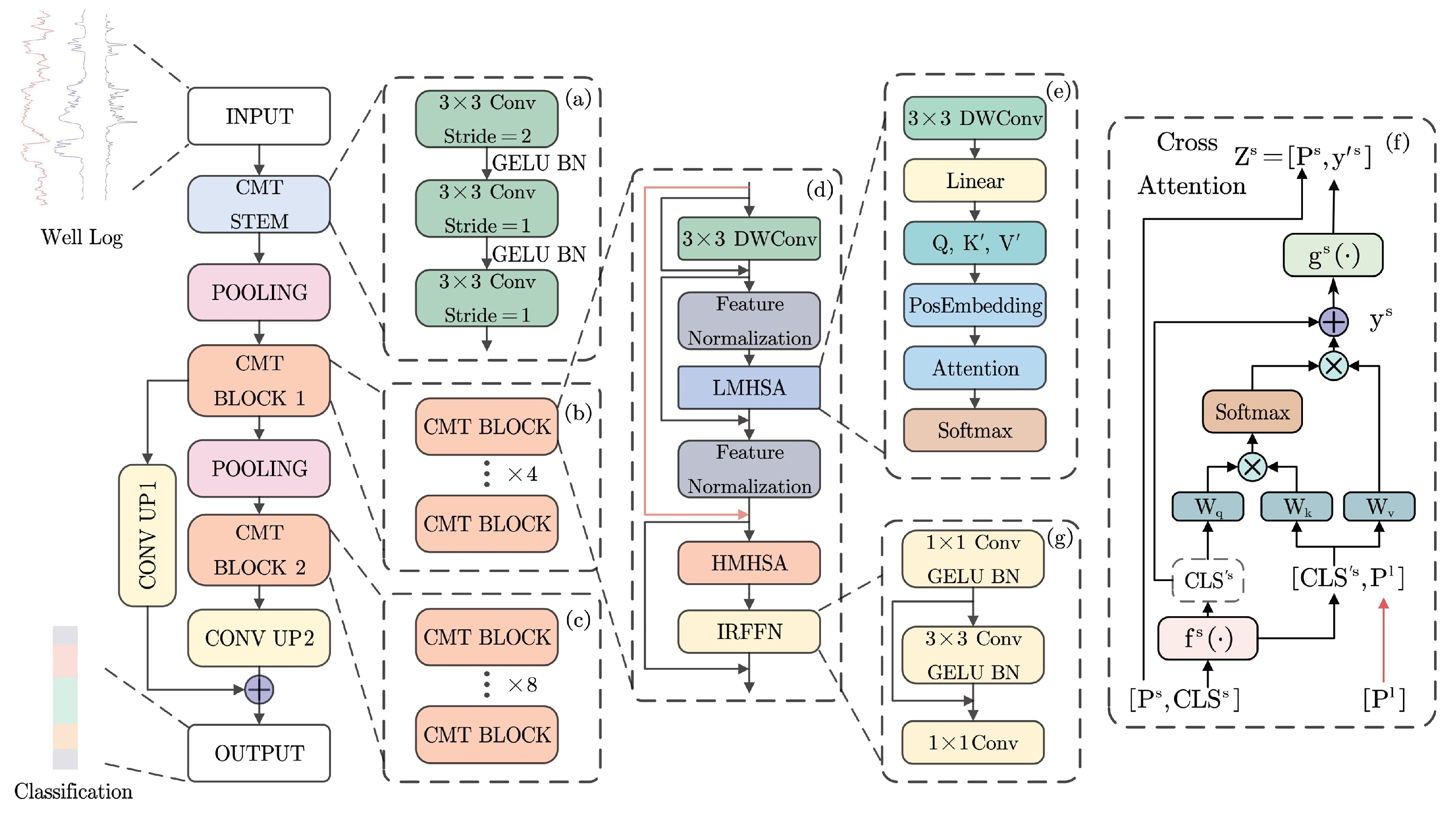
2. Methodology
2.1. The Architecture of CMT-Enhanced Hiformer
2.1.1. CMTSTEM Module
2.1.2. CMTBLOCK Module
2.1.3. CONVUP Module
2.2. Loss Function with Geological Constraint
3. Data Introduction and Implementation Details
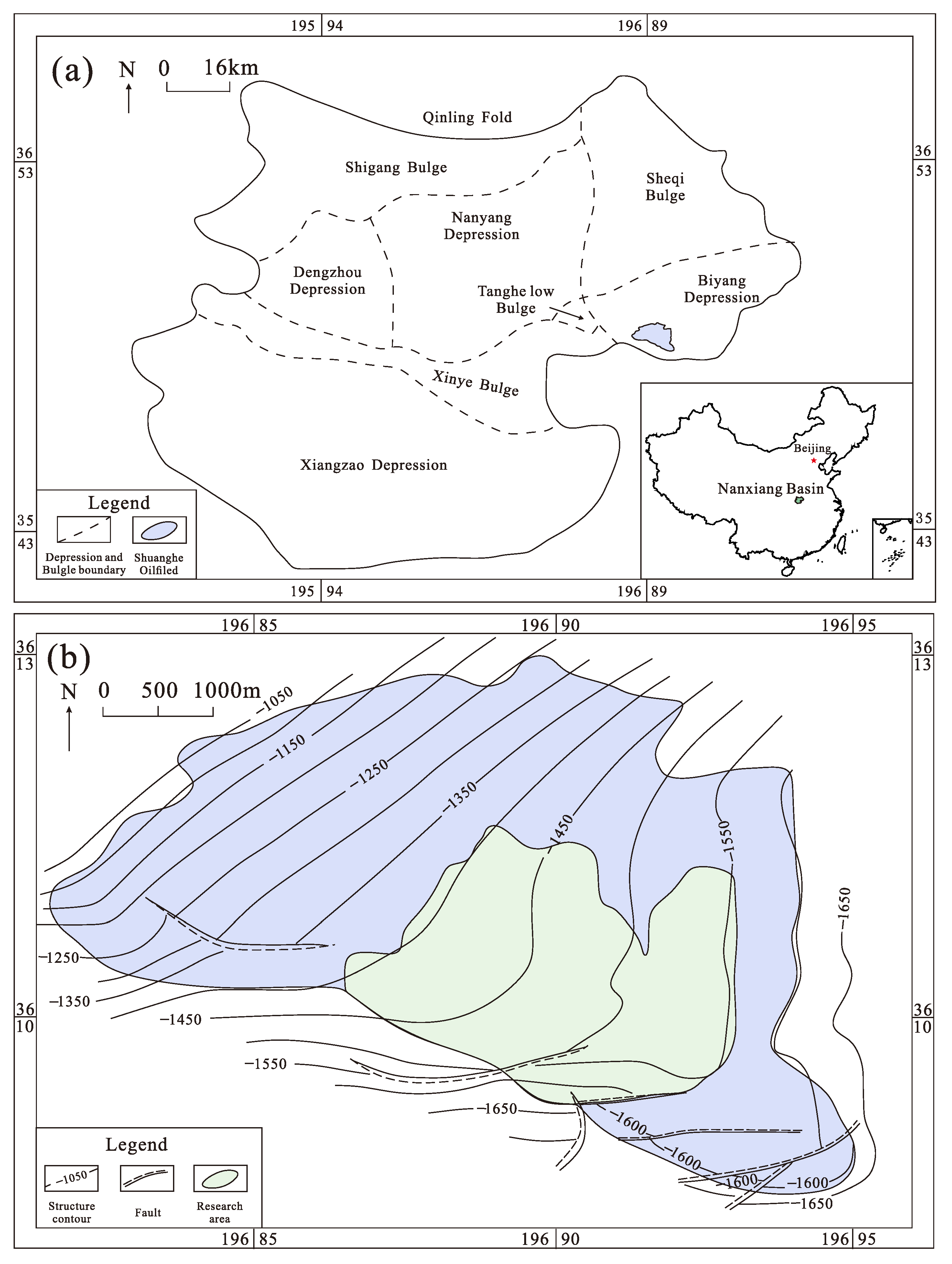
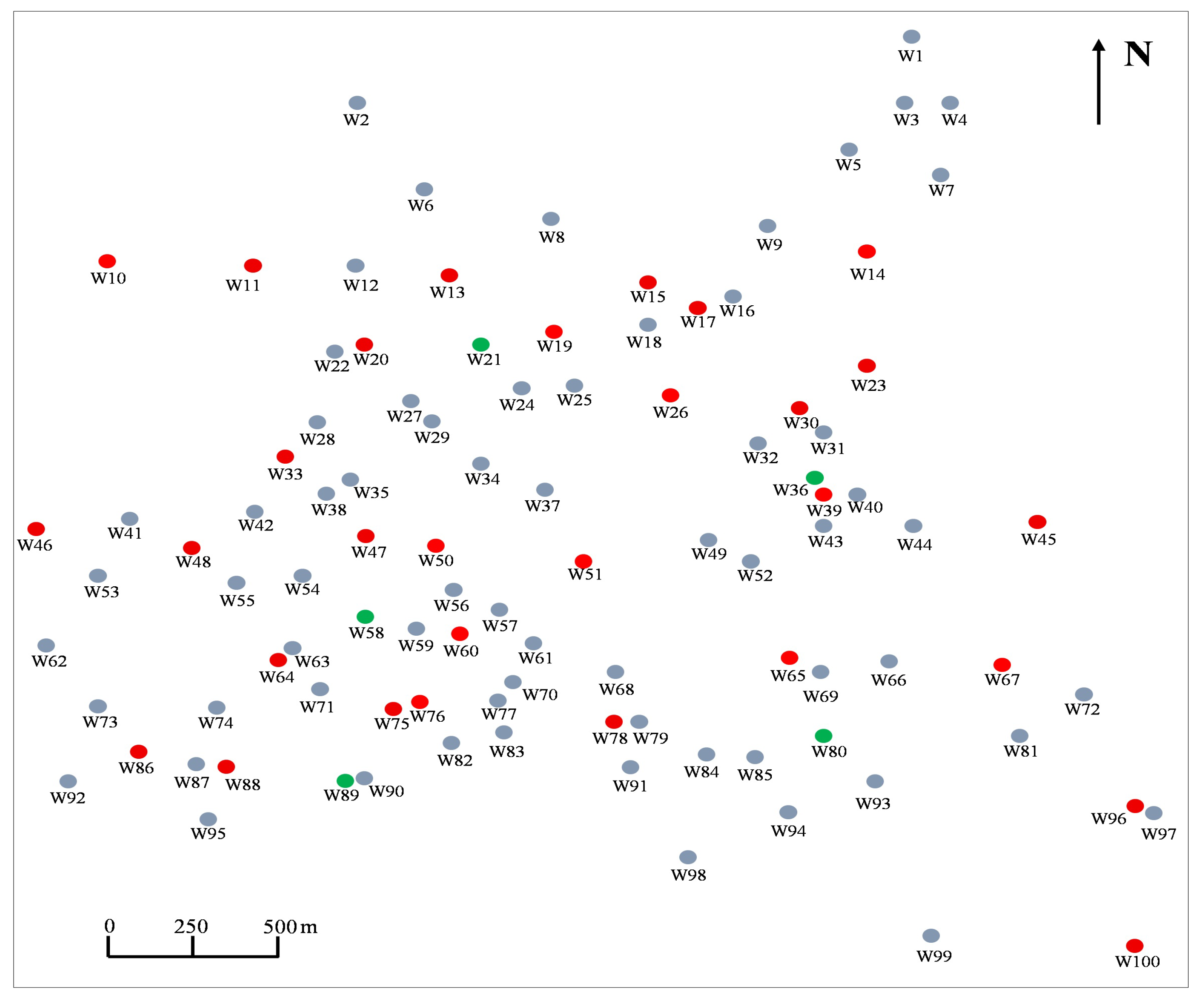
3.1. Study Area and Training Data Preparation
3.2. Implementation Details of Training Process
4. Ablation Study
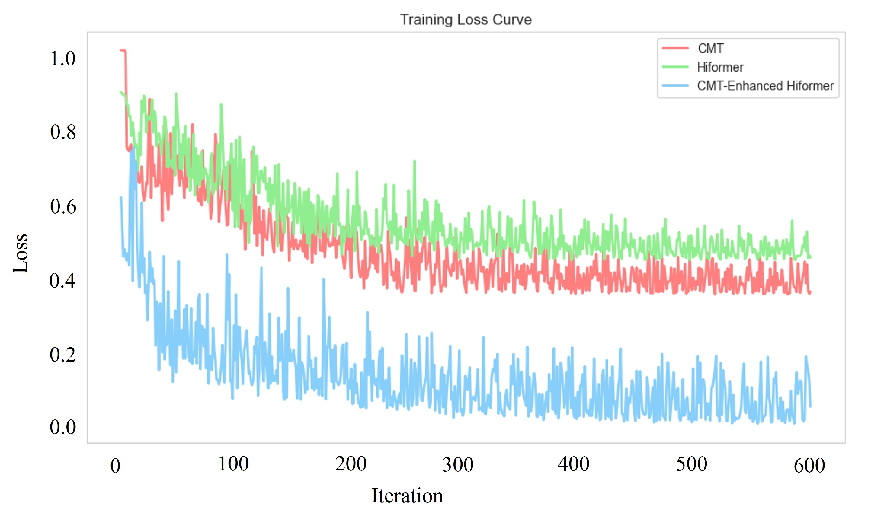
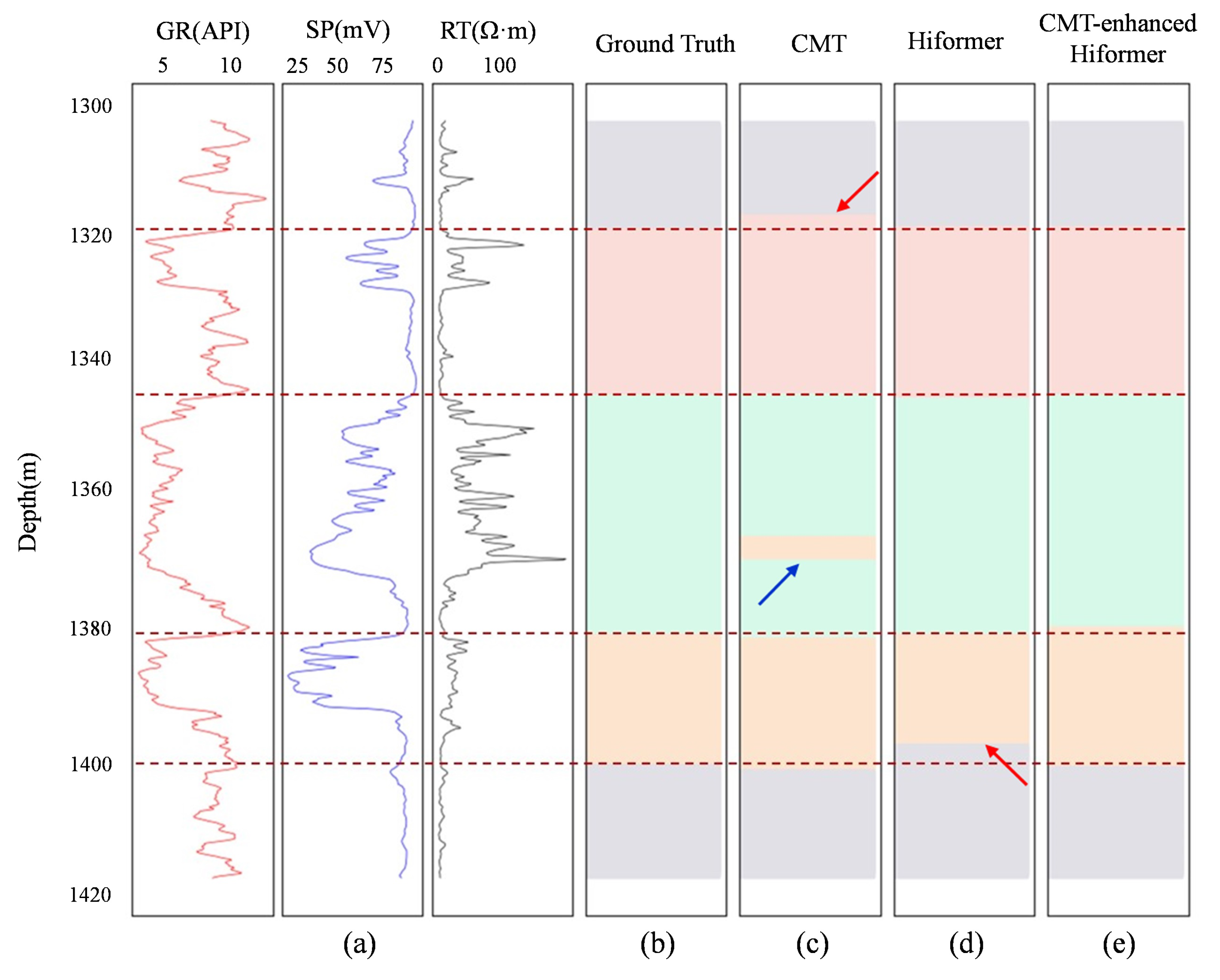
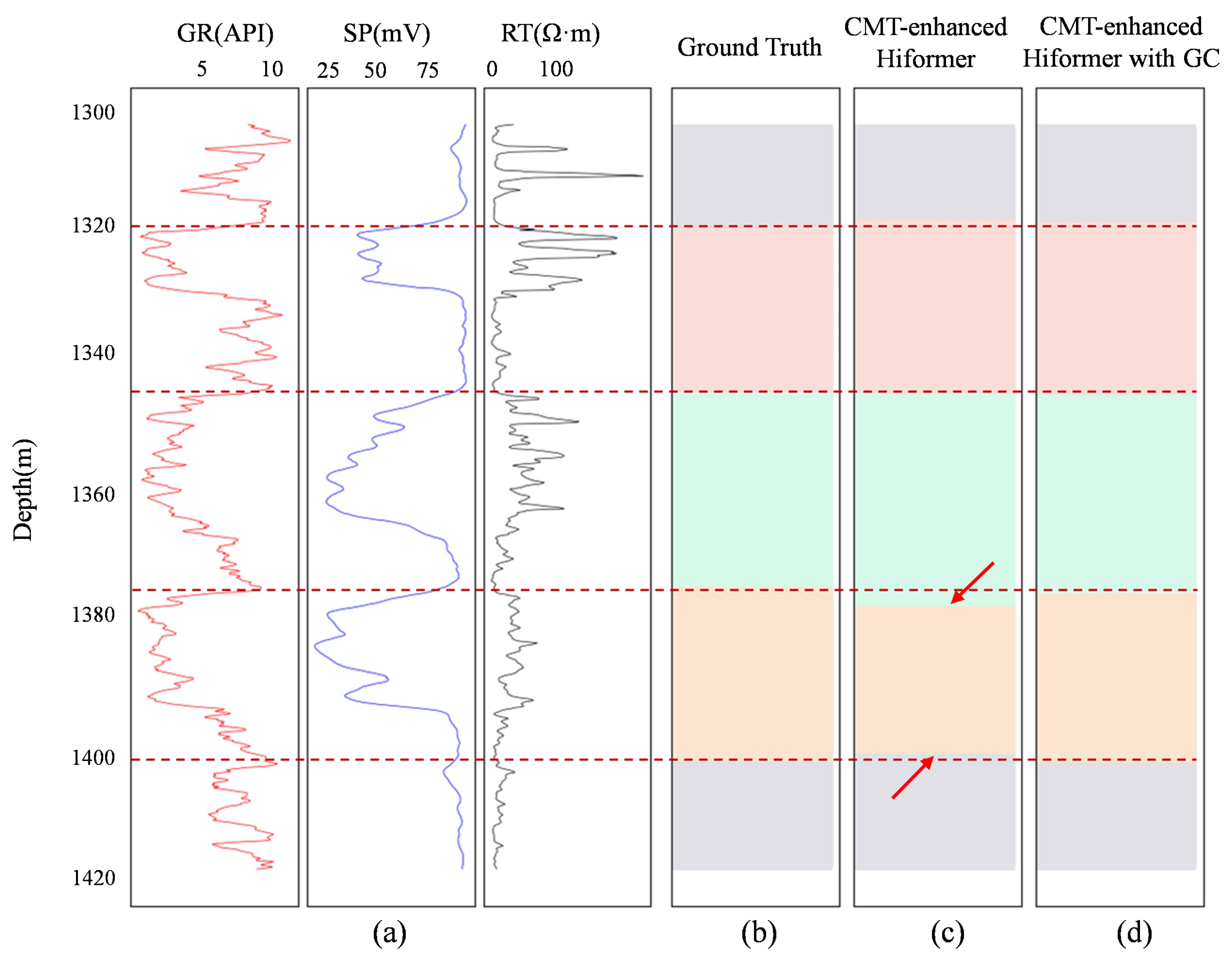
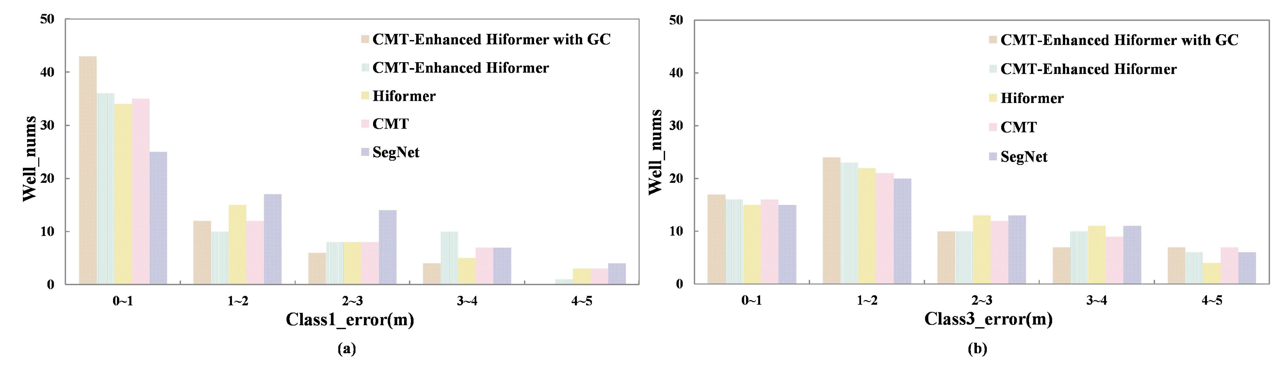
4.1. The Comparisons of Different Modules
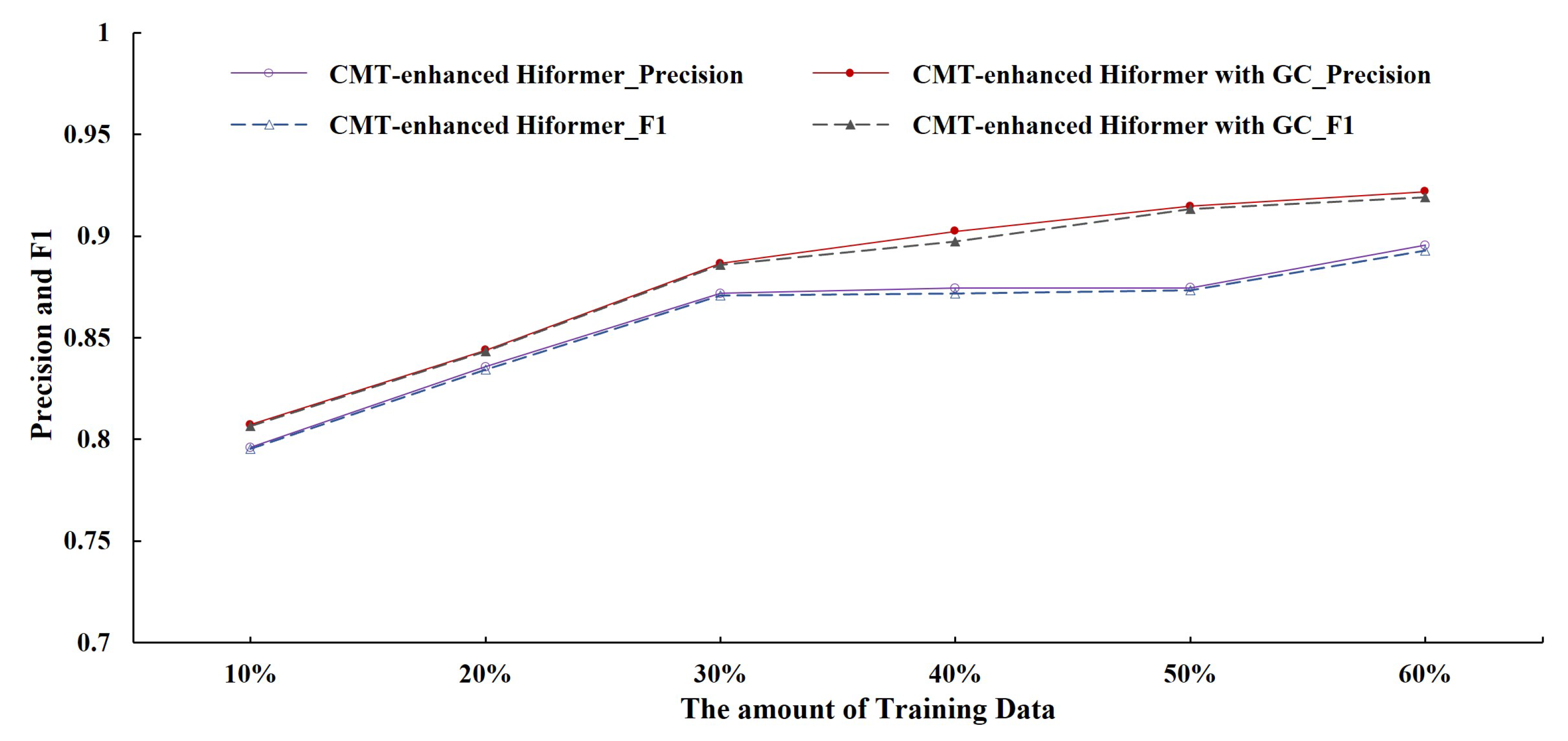
4.2. The Comparisons of Different Regularization Weights
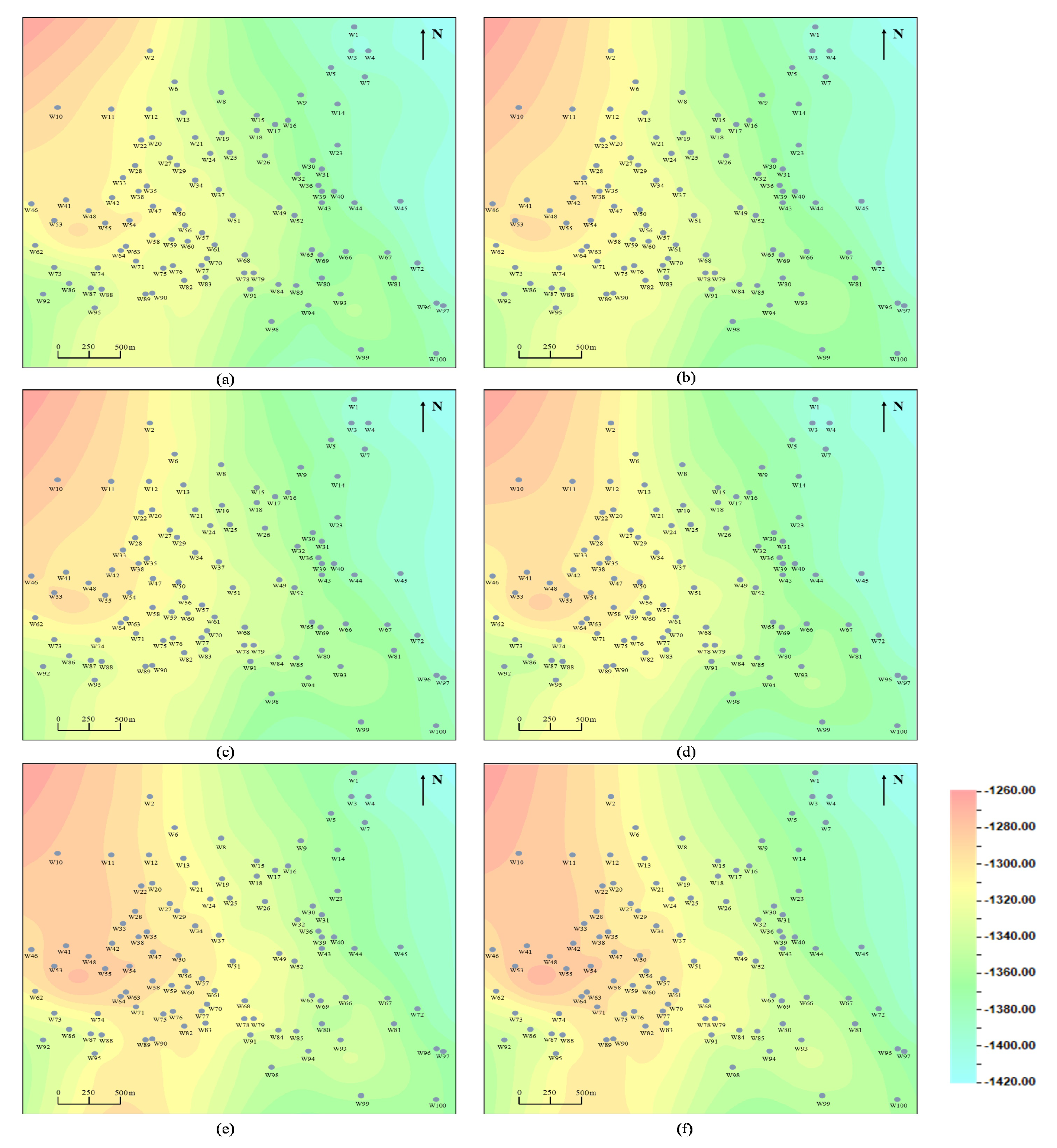
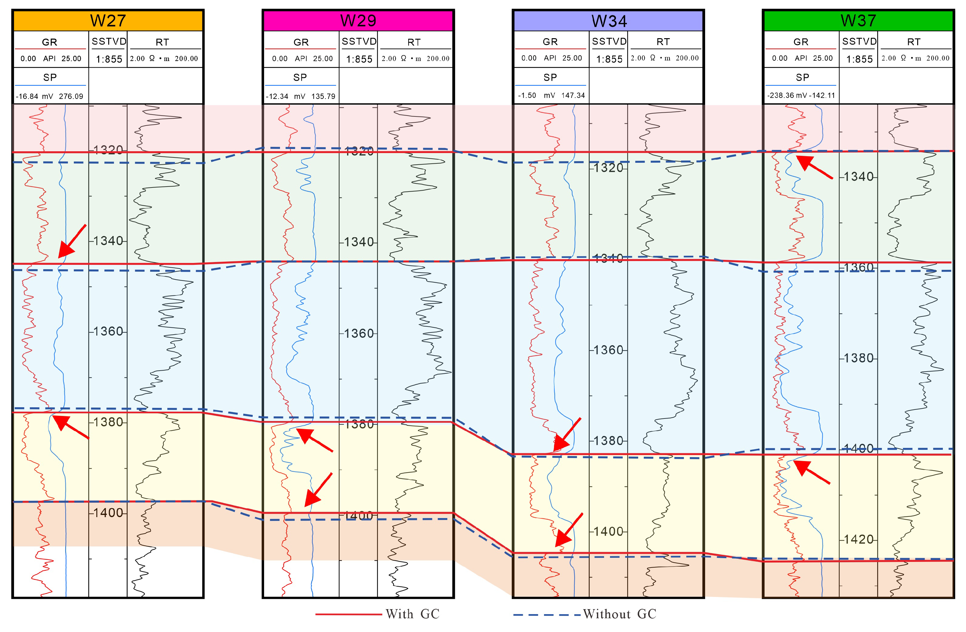
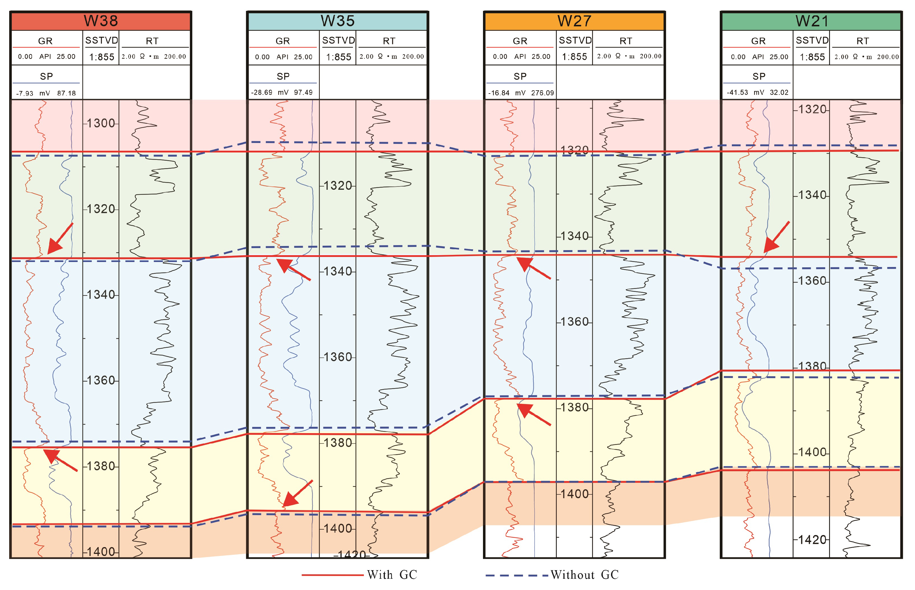
5. Stratigraphic Correlation Results
6. Discussion
7. Conclusions
Author Contributions
Funding
Data Availability Statement
Acknowledgments
Conflicts of Interest
References
- Liu, Y.; Shi, C.; Wu, Q.; Zhang, R.; Zhou, Z. Visual analytics of stratigraphic correlation for multi-attribute well-logging data exploration. IEEE Access 2019, 7, 98122–98135. [Google Scholar] [CrossRef]
- Dai, Y.; Huang, X.; Liu, H.; Yang, H.; Wei, G.; Lu, N.; Han, Z.; Song, H. Stratigraphic automatic correlation using SegNet semantic segmentation model. In Proceedings of the SEG/AAPG/SEPM First International Meeting for Applied Geoscience & Energy, Denver, CO, USA, 26 September–1 October 2021; p. D011S065R003. [Google Scholar]
- Partovi, S.M.A.; Sadeghnejad, S. Fractal parameters and well-logs investigation using automated well-to-well correlation. Comput. Geosci. 2017, 103, 59–69. [Google Scholar] [CrossRef]
- Liang, J.; Wang, H.; Blum, M.J.; Ji, X. Demarcation and correlation of stratigraphic sequences using wavelet and Hilbert-Huang transforms: A case study from Niger Delta Basin. J. Pet. Sci. Eng. 2019, 182, 106329. [Google Scholar] [CrossRef]
- Kadkhodaie, A.; Rezaee, R. Intelligent sequence stratigraphy through a wavelet-based decomposition of well log data. J. Nat. Gas Sci. Eng. 2017, 40, 38–50. [Google Scholar] [CrossRef]
- Xu, Z.; Zhang, B.; Li, F.; Cao, G.; Liu, Y. Well-log decomposition using variational mode decomposition in assisting the sequence stratigraphy analysis of a conglomerate reservoir. Geophysics 2018, 83, B221–B228. [Google Scholar] [CrossRef]
- Al-Baldawi, B.A.H. Using well logs data in Logfacies determination by applying the cluster analysis technique for Khasib Formation, Amara oil field, south Eastern Iraq. J. Pet. Res. Stud. 2016, 6, 9–26. [Google Scholar] [CrossRef]
- Karimi, A.M.; Sadeghnejad, S.; Rezghi, M. Well-to-well correlation and identifying lithological boundaries by principal component analysis of well-logs. Comput. Geosci. 2021, 157, 104942. [Google Scholar] [CrossRef]
- Ma, Y.Z. Lithofacies clustering using principal component analysis and neural network: Applications to wireline logs. Math. Geosci. 2011, 43, 401–419. [Google Scholar] [CrossRef]
- Vincent, P.; Gartner, J.; Attali, G. An approach to detailed dip determination using correlation by pattern recognition. J. Pet. Technol. 1979, 31, 232–240. [Google Scholar] [CrossRef]
- Behdad, A. A step toward the practical stratigraphic automatic correlation of well logs using continuous wavelet transform and dynamic time warping technique. J. Appl. Geophys. 2019, 167, 26–32. [Google Scholar] [CrossRef]
- Fang, H.; Lou, Y.; Zhang, B.; Xu, H.; Lu, M. Mimicking the process of manual sequence stratigraphy well correlation. Interpretation 2021, 9, T667–T684. [Google Scholar] [CrossRef]
- Wang, C.; Wei, X.; Pan, H.; Han, L.; Wang, H.; Wang, H.; Zhao, H. Well Logging Stratigraphic Correlation Algorithm Based on Semantic Segmentation. Appl. Geophys. 2024, 21, 650–666. [Google Scholar] [CrossRef]
- Rudman, A.J.; Lankston, R.W. Stratigraphic correlation of well logs by computer techniques. Aapg Bull. 1973, 57, 577–588. [Google Scholar]
- Mehta, C.; Radhakrishnan, S.; Srikanth, G. Segmentation of well logs by maximum-likelihood estimation. Math. Geol. 1990, 22, 853–869. [Google Scholar] [CrossRef]
- Wang, X.; Du, M.; Yu, W. Application of grey correlation method for stratigraphic correlation and its improvements. Well Logging Technol. 2006, 30, 126. [Google Scholar]
- Zhang, T.; Plotnick, R.E. Graphic Biostratigraphic Correlation Using Genetic Algorithms. Math. Geol. 2006, 38, 781–800. [Google Scholar] [CrossRef]
- Hohn, M.E.; Fontana, M.V. Geostatistics and artificial intelligence applied to stratigraphic correlation. Am. Assoc. Pet. Geol. Conv. 1986, 70, 5201053. [Google Scholar]
- Parimontonsakul, M.; Lotongkum, S.; Mularlee, K. A machine learning based approach to automate stratigraphic correlation through marker determination. Improv. Oil Gas Recovery 2023, 7, IOGR.1204. [Google Scholar] [CrossRef]
- Tognoli, F.M.W.; Spaniol, A.F.; Mello, M.E.D.; Souza, L.V.d. A machine-learning based approach to predict facies associations and improve local and regional stratigraphic correlations. Mar. Pet. Geol. 2024, 160, 19. [Google Scholar] [CrossRef]
- Malmgren, B.A.; Nordlund, U. Application of Artificial Neural Networks to Stratigraphic Correlation. Paleontol. Soc. Spec. Publ. 1996, 8, 257. [Google Scholar] [CrossRef]
- Tokpanov, Y.; Smith, J.; Ma, Z.; Deng, L.; Benhallam, W.; Salehi, A.; Zhai, X.; Darabi, H.; Castineira, D. Deep-learning-based automated stratigraphic correlation. In Proceedings of the SPE Annual Technical Conference and Exhibition, Virtual, 26–29 October 2020; p. D022S061R020. [Google Scholar]
- Gu, X.; Lu, W.; Li, Y.; Wang, Y. Semi-supervised seismic stratigraphic interpretation constrained by spatial structure. IEEE Trans. Geosci. Remote Sens. 2023, 61, 5912710. [Google Scholar] [CrossRef]
- Jiang, C.; Zhang, D.; Chen, S. Lithology identification from well-log curves via neural networks with additional geologic constraint. Geophysics 2021, 86, IM85–IM100. [Google Scholar] [CrossRef]
- Wang, D.; Chen, G. Intelligent seismic stratigraphic modeling using temporal convolutional network. Comput. Geosci. 2023, 171, 105294. [Google Scholar] [CrossRef]
- Yuan, S.; Liu, J.; Wang, S.; Wang, T.; Shi, P. Seismic waveform classification and first-break picking using convolution neural networks. IEEE Geosci. Remote Sens. Lett. 2018, 15, 272–276. [Google Scholar] [CrossRef]
- Feng, R.; Balling, N.; Grana, D.; Dramsch, J.S.; Hansen, T.M. Bayesian convolutional neural networks for seismic facies classification. IEEE Trans. Geosci. Remote Sens. 2021, 59, 8933–8940. [Google Scholar] [CrossRef]
- Pardo, E.; Garfias, C.; Malpica, N. Seismic phase picking using convolutional networks. IEEE Trans. Geosci. Remote Sens. 2019, 57, 7086–7092. [Google Scholar] [CrossRef]
- Hu, G.; Hu, Z.; Liu, J.; Cheng, F.; Peng, D. Seismic fault interpretation using deep learning-based semantic segmentation method. IEEE Geosci. Remote Sens. Lett. 2020, 19, 7500905. [Google Scholar] [CrossRef]
- Ferreira, R.S.; Oliveira, D.A.; Semin, D.G.; Zaytsev, S. Automatic velocity analysis using a hybrid regression approach with convolutional neural networks. IEEE Trans. Geosci. Remote Sens. 2020, 59, 4464–4470. [Google Scholar] [CrossRef]
- Liu, N.; Lei, Y.; Yang, Y.; Wei, S.; Gao, J.; Jiang, X. Self-supervised time-frequency representation based on generative adversarial networks. Geophysics 2023, 88, IM87–IM99. [Google Scholar] [CrossRef]
- Torres, J.F.; Hadjout, D.; Sebaa, A.; Martínez-Álvarez, F.; Troncoso, A. Deep learning for time series forecasting: A survey. Big Data 2021, 9, 3–21. [Google Scholar] [CrossRef]
- Raghu, M.; Unterthiner, T.; Kornblith, S.; Zhang, C.; Dosovitskiy, A. Do vision transformers see like convolutional neural networks? Adv. Neural Inf. Process. Syst. 2021, 34, 12116–12128. [Google Scholar]
- Liu, N.; Huo, J.; Li, Z.; Wu, H.; Lou, Y.; Gao, J. Seismic attributes aided horizon interpretation using an ensemble dense inception transformer network. IEEE Trans. Geosci. Remote Sens. 2024, 62, 5902010. [Google Scholar] [CrossRef]
- Vaswani, A. Attention is all you need. arXiv 2017, arXiv:1706.03762. [Google Scholar]
- Liu, C.; Zhao, R.; Shi, Z. Remote-sensing image captioning based on multilayer aggregated transformer. IEEE Geosci. Remote Sens. Lett. 2022, 19, 6506605. [Google Scholar] [CrossRef]
- Zerveas, G.; Jayaraman, S.; Patel, D.; Bhamidipaty, A.; Eickhoff, C. A transformer-based framework for multivariate time series representation learning. In Proceedings of the 27th ACM SIGKDD Conference on Knowledge Discovery & Data Mining, Virtual Event, Singapore, 14–18 August 2021; pp. 2114–2124. [Google Scholar]
- Liu, Z.; Lin, Y.; Cao, Y.; Hu, H.; Wei, Y.; Zhang, Z.; Lin, S.; Guo, B. Swin transformer: Hierarchical vision transformer using shifted windows. In Proceedings of the IEEE/CVF International Conference on Computer Vision, Montreal, BC, Canada, 11–17 October 2021; pp. 10012–10022. [Google Scholar]
- Heidari, M.; Kazerouni, A.; Soltany, M.; Azad, R.; Aghdam, E.K.; Cohen-Adad, J.; Merhof, D. Hiformer: Hierarchical multi-scale representations using transformers for medical image segmentation. In Proceedings of the IEEE/CVF Winter Conference on Applications of Computer Vision, Waikoloa, HI, USA, 2–7 January 2023; pp. 6202–6212. [Google Scholar]
- Guo, J.; Han, K.; Wu, H.; Tang, Y.; Chen, X.; Wang, Y.; Xu, C. Cmt: Convolutional neural networks meet vision transformers. In Proceedings of the IEEE/CVF Conference on Computer Vision and Pattern Recognition, New Orleans, LA, USA, 18–24 June 2022; pp. 12175–12185. [Google Scholar]
- Xu, K.; Chen, H.; Huang, C.; Ogg, J.G.; Zhu, J.; Lin, S.; Yang, D.; Zhao, P.; Kong, L. Astronomical time scale of the Paleogene lacustrine paleoclimate record from the Nanxiang Basin, central China. Palaeogeogr. Palaeoclimatol. Palaeoecol. 2019, 532, 109253. [Google Scholar] [CrossRef]
- Su, A.; Chen, H.; Zhao, J.; Feng, Y.; Nguyen, A.D. Exhumation filling and paleo-pasteurization of the shallow petroleum system in the North Slope of the Biyang Sag, Nanxiang Basin, China. Mar. Pet. Geol. 2021, 133, 105267. [Google Scholar] [CrossRef]
- Su, A.; Chen, H.; Zhao, J.; Feng, Y. Integrated fluid inclusion analysis and petrography constraints on the petroleum system evolution of the central and southern Biyang Sag, Nanxiang Basin, Eastern China. Mar. Pet. Geol. 2020, 118, 104437. [Google Scholar] [CrossRef]
- Dong, Y.; Zhu, X.; Xian, B.; Hu, T.; Geng, X.; Liao, J.; Luo, Q. Seismic geomorphology study of the Paleogene Hetaoyuan Formation, central-south Biyang Sag, Nanxiang Basin, China. Mar. Pet. Geol. 2015, 64, 104–124. [Google Scholar] [CrossRef]

| Methods | Precision | F1 |
|---|---|---|
| CMT | 0.8365 | 0.8357 |
| Hiformer | 0.8277 | 0.8271 |
| CMT-enhanced Hiformer | 0.8717 | 0.8708 |
| Weight | Precision | F1 |
|---|---|---|
| = 1, = 0 | 0.8717 | 0.8708 |
| = 0.95, = 0.05 | 0.8433 | 0.8414 |
| = 0.90, = 0.10 | 0.8571 | 0.8567 |
| = 0.85, = 0.15 | 0.8735 | 0.8731 |
| = 0.80, = 0.20 | 0.8865 | 0.8857 |
| = 0.75, = 0.25 | 0.8759 | 0.8749 |
| = 0.70, = 0.30 | 0.8489 | 0.8480 |
| Methods | Average Differences (m) |
|---|---|
| SegNet | 2.91 |
| CMT | 2.23 |
| Hiformer | 2.54 |
| CMT-enhanced Hiformer | 1.85 |
| CMT-enhanced Hiformer with GC | 1.39 |
Disclaimer/Publisher’s Note: The statements, opinions and data contained in all publications are solely those of the individual author(s) and contributor(s) and not of MDPI and/or the editor(s). MDPI and/or the editor(s) disclaim responsibility for any injury to people or property resulting from any ideas, methods, instructions or products referred to in the content. |
© 2025 by the authors. Licensee MDPI, Basel, Switzerland. This article is an open access article distributed under the terms and conditions of the Creative Commons Attribution (CC BY) license (https://creativecommons.org/licenses/by/4.0/).
Share and Cite
Xu, Z.; Zheng, B.; Liu, B.; Song, W. Stratigraphic Correlation of Well Logs Using Geology-Informed Deep Learning Networks. Processes 2025, 13, 1288. https://doi.org/10.3390/pr13051288
Xu Z, Zheng B, Liu B, Song W. Stratigraphic Correlation of Well Logs Using Geology-Informed Deep Learning Networks. Processes. 2025; 13(5):1288. https://doi.org/10.3390/pr13051288
Chicago/Turabian StyleXu, Zhaohui, Boyu Zheng, Bo Liu, and Wendan Song. 2025. "Stratigraphic Correlation of Well Logs Using Geology-Informed Deep Learning Networks" Processes 13, no. 5: 1288. https://doi.org/10.3390/pr13051288
APA StyleXu, Z., Zheng, B., Liu, B., & Song, W. (2025). Stratigraphic Correlation of Well Logs Using Geology-Informed Deep Learning Networks. Processes, 13(5), 1288. https://doi.org/10.3390/pr13051288