Prediction of Mud Weight Window Based on Geological Sequence Matching and a Physics-Driven Machine Learning Model for Pre-Drilling

Abstract

Accurate pre-drilling mud weight window (MWW) prediction is crucial for drilling fluid design and wellbore stability in complex geological formations. Traditional physics-based approaches suffer from subjective parameter selection and inadequate handling of multi-mechanism over-pressured formations, while machine learning methods lack physical constraints and interpretability. This study develops a novel physics-guided deep learning framework integrating rock mechanics theory with deep neural networks for enhanced MWW prediction. The framework incorporates three key components: first, a physics-driven layer synthesizing intermediate variables from rock physics calculations to embed domain knowledge while preserving interpretability; second, a geological sequence-matching algorithm enabling precise stratigraphic correlation between offset and target wells, compensating for lateral geological heterogeneity; third, a long short-term memory network capturing sequential drilling characteristics and geological structure continuity. Case study results from 12 wells in northwestern China demonstrate significant improvements over traditional methods: collapse pressure prediction error reduced by 40.96%, pore pressure error decreased by 30.43%, and fracture pressure error diminished by 39.02%. The proposed method successfully captures meter-scale pressure variations undetectable by conventional approaches, providing critical technical support for wellbore design optimization, drilling fluid formulation, and operational safety enhancement in challenging geological environments.

1. Introduction

The mud weight window (MWW) directly determines wellbore stability, well control safety, and wellbore integrity [1,2] serving as the core foundation for drilling fluid density design, casing program optimization, and well control contingency planning. Inaccurate estimation can readily trigger high-risk events such as lost circulation, kicks, or even blowouts [3] resulting in substantial economic losses and environmental disasters. Therefore, accurate MWW prediction is not only a prerequisite for safe drilling and completion operations in complex formations but also a critical guarantee for enhancing the success rate of oil and gas resource development [4].

Since the 1970s, the industry has primarily relied on physics-based empirical models (such as the Eaton method and Bowers approach) to estimate formation pore pressure by establishing correlations between sonic transit time and vertical effective stress. These methods combine formation strength parameters with Mohr–Coulomb or Drucker–Prager failure criteria to determine collapse pressure and fracture pressure, ultimately providing the mud weight range. Foster proposed the equivalent depth method, establishing normal trend lines for formation factors to determine effective stress and pore pressure [5]. Pennebaker introduced overlay charts using seismic interval velocities, improving prediction accuracy but lacking consideration for lithological and geological age variations [6]. Eaton combined Terzaghi’s effective stress principle to develop the widely used Eaton method, though subjective bias in determining normal trend lines and empirical parameters affect accuracy [7,8]. Bowers incorporated loading and unloading mechanisms to predict abnormal pressures from different geological processes [9]. Concurrently, researchers have conducted extensive studies on mud weight window optimization and wellbore stability analysis in shale formations. Zhang modified the Biot effective stress principle, integrating Weibull statistical and flow–diffusion coupling models to calculate safe drilling fluid densities for shale formations considering sealing inhibition-reverse osmosis effects [10]. Kadkhodaie developed an improved wellbore stability analysis method for Iranian Persian Gulf offshore fields by combining geomechanical unit classification, FMI log interpretation, and rock mechanics testing [11]. Liu established an elastoplastic mud weight window determination method incorporating thermo-mechanical coupling effects, demonstrating opposite correlations between mud weight windows and geothermal gradients at different depth intervals [12]. Zhang proposed an elastoplastic collapse pressure model based on the Hoek–Brown strength criterion, incorporating the plastic zone radius, geological strength index, non-uniform in situ stress coefficient, and rock uniaxial compressive strength for deep coal seam drilling applications [13]. Existing research primarily focuses on normal compaction trend (NCT) fitting optimization, rock strength parameter determination, and regional empirical coefficient modification, achieving significant progress under specific geological conditions. However, these traditional methods face numerous challenges that affect their accuracy and reliability in complex environments. First, conventional single-compaction mechanism models inadequately characterize over-pressured formations generated by multi-mechanism processes (rapid sedimentation, tectonic unloading, and fault sealing), introducing systematic bias in pore pressure inversion. Second, traditional depth-based well correlation methods neglect inter-well stratigraphic sequence variations and thickness changes, yielding poor prediction accuracy in fault-intensive or heterogeneous regions where errors amplify exponentially. Third, while seismic prediction provides spatial coverage, resolution constraints and velocity inversion uncertainties limit vertical formation pressure characterization, particularly in deep, structurally complex areas where depth-dependent error amplification compromises mud weight window reliability.

In recent years, machine learning (ML), particularly through deep learning (DL) techniques, has demonstrated superior performance in rock physics parameter inversion and real-time drilling optimization. Multiple researchers have employed models such as random forest, XGBoost, and LSTM to train on logging, mud logging, and real-time drilling data, achieving rapid prediction of mud weight windows. Song developed an LSTM-BP neural network method targeting drilling and sedimentation sequences, demonstrating superior accuracy compared to individual BP, LSTM, and SVM models for intelligent tri-pressure prediction [14]. Deng established the IGWO-MLP intelligent prediction method by integrating machine learning algorithms with effective stress theory, showing excellent generalization capability across three-well validation datasets [15]. Li proposed a LightGBM-based intelligent prediction model using well depth, formation density, and pore pressure equivalent density as inputs, achieving superior accuracy and stability compared to sonic logging methods in S block vertical wells [16]. Zhang introduced an adaptive physics-informed deep learning model (CGP-NN) for direct pore pressure prediction from seismic data, incorporating 1DCPP feature extraction, multi-layer GRU, and adaptive physics-informed loss functions for multi-genetic mechanism prediction [17]. Chen embedded rock physics theory into GRU and LSTM models using seismic and logging-while-drilling (LWD) data, combined with SHAP interpretation methods for accurate prediction and model optimization guidance [18]. Hussain developed a hybrid SOM-MLP-SSD model for predicting missing well-log data, particularly shear wave transit time, using lithofacies classification and parameter optimization, significantly outperforming traditional methods in complex zones [19]. Doyoro applied k-means clustering to post-process seismic refraction and electrical resistivity tomography data, enhancing geological structure detection and fault delineation compared to conventional interpretation methods [20]. Wang proposed a deep learning approach for identifying geological discontinuities in borehole images, demonstrating SegFormer’s superiority over U-Net and improving model robustness through weighted loss functions for automated geological interpretation [21].

However, the aforementioned studies suffer from several critical limitations. First, high-quality pore pressure measurements are costly and limited, resulting in small datasets with high noise levels that increase overfitting susceptibility. Second, essential logging parameters (sonic transit time, density, resistivity) are unavailable prior to drilling, forcing reliance on regional seismic or offset well extrapolation that inadequately accounts for spatial geological variations and significantly increases prediction uncertainty. Third, mud-logging data suffer from substantial interference noise caused by drill string mechanical vibrations, annular clearances, circulation effects, and cutting lag time, leading to poor depth–time alignment and inability to detect thin bed anomalies or stress variations. Finally, while LWD provides near-wireline accuracy with real-time capabilities, its adoption remains limited due to high operational costs and insufficient mud pulse/electromagnetic transmission bandwidth for complete waveform data transfer, preventing high-dimensional feature extraction.

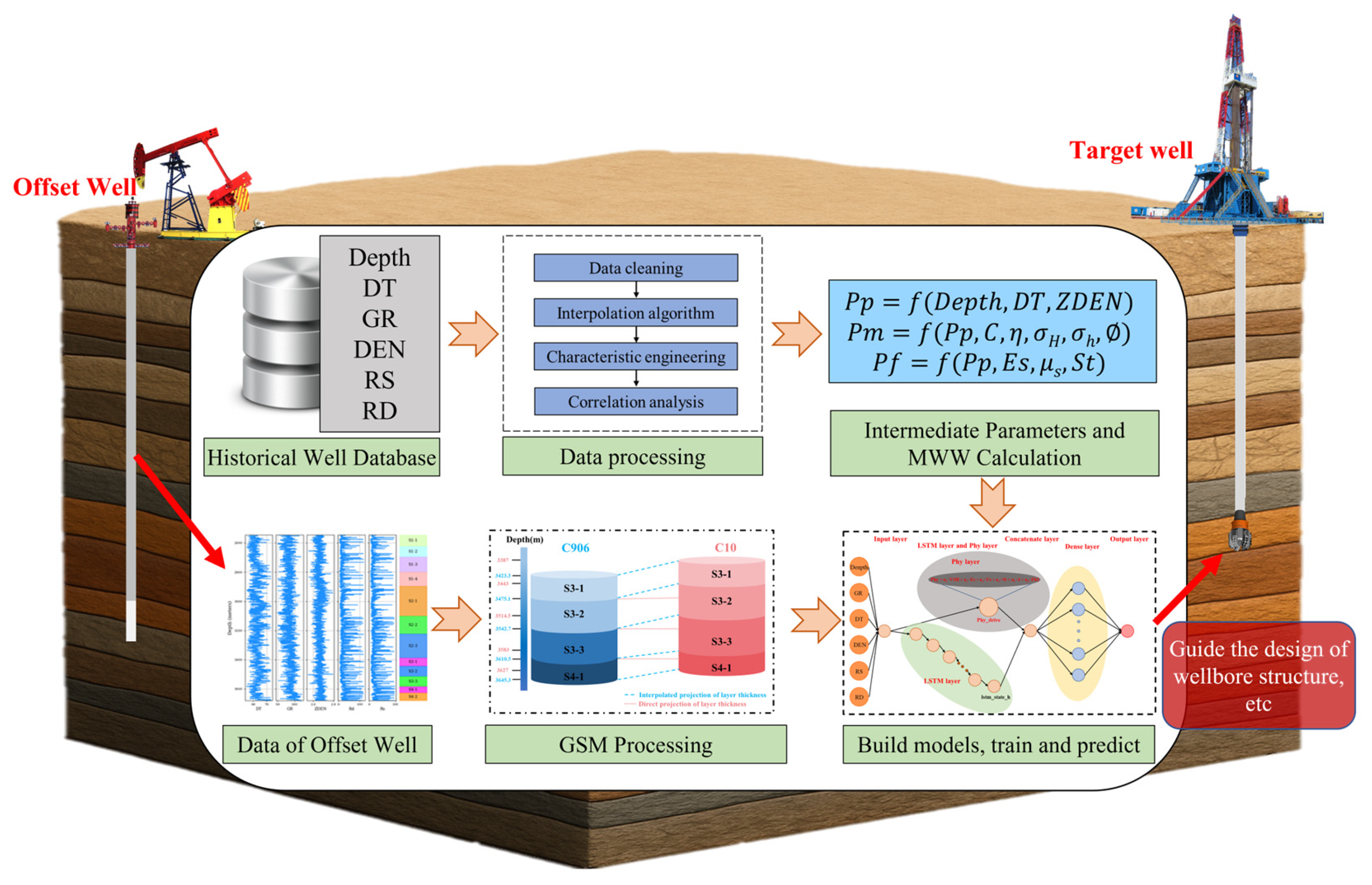
Based on the aforementioned challenges, this study develops a physics-guided mud weight window estimation model and demonstrates its superiority through case studies of 12 wells in Block C of a northwestern China oilfield. As illustrated in Figure 1, the workflow of this methodology begins with statistical analysis of historical well data in the target block, combining rock mechanics models, drilling fluid density usage, and actual complex conditions to calculate estimated mud weight window values. Following the approach of rock mechanics theory and empirical formulas for stepwise calculation of rock mechanical parameters, an LSTM algorithm is employed to train a physics-guided mud weight window estimation model. Finally, geological sequence matching (GSM) is applied to offset wells to obtain high-precision pre-drilling geological estimation parameters for the target well, which are subsequently input into the model for mud weight window prediction of the target well.

2. Data and Theory

2.1. Data Overview

The case study data originates from Block C of a northwestern China oilfield. This block contains 12 wells, with well C10 serving as the target well. The well locations and fault distribution are shown in Figure 2a, while the comprehensive stratigraphic column is presented in Figure 2b [22]. This block belongs to a nose-shaped structure containing four faults of varying scales. Faults 1, 2, and 3 exhibit similar strike orientations with poor sealing capacity. The area has developed four oil-bearing formations—S1, S2, S3, and S4—with the S2 formation serving as the main productive reservoir. The S1 oil group consists of calcareous mudstone and oil shale in the middle section, gray mudstone and siltstone in the upper section, and brown-yellow sandstone and gray siltstone interbedded with calcareous mudstone in the lower section. The upper part of the S2 oil group develops gray-green and gray sandstone interbedded with calcareous sandstone and conglomeratic sandstone, while the lower part is dominated by brown-yellow sandstone and mudstone interbedded with gray and dark gray carbonate rocks. The lower section of the S3 oil group primarily develops dark organic-rich dolomitic limestone, with the upper section featuring superimposed gray dolomite and argillaceous dolomitic limestone interbedded with multiple salt rock layers. The S4 oil group is predominantly composed of brown-red and brown mudstone, sandy mudstone, and fine sandstone, with secondary gray and gray-yellow siltstone, argillaceous siltstone, and conglomeratic sandstone and conglomerate developed at the bottom. Through detailed subdivision, the S1 formation can be divided into four sublayers (S1-1, S1-2, S1-3, S1-4), the S2 formation into three sublayers (S2-1, S2-2, S2-3), the S3 formation into three sublayers (S3-1, S3-2, S3-3), and the S4 formation into two sublayers (S4-1, S4-2).

In this study, we collected six logging parameters from twelve wells (depth, sonic transit time (DT, μs/ft), deep-investigated double lateral resistivity log (Rd, Ω·m), shallow-investigated double lateral resistivity log (Rs, Ω·m), natural gamma ray (GR, gAPI), and bulk density (ZDEN, g/cm³)), along with fifteen theoretically calculated parameters, which were shale content (Vsh, %), P-wave velocity (Vp, m/s), dynamic elastic modulus (Ed, MPa), static elastic modulus (Es, MPa), dynamic Poisson’s ratio (Ud, dimensionless), static Poisson’s ratio (Us, dimensionless), uniaxial compressive strength (Sc, MPa), tensile strength (St, MPa), cohesion (C, MPa), internal friction angle (J, °), minimum principal stress (σ_h, MPa), maximum principal stress (σ_H,, MPa), pore pressure (Pp, g/cm³), collapse pressure (Pm, g/cm³), and fracture pressure (Pf, g/cm³), totaling 1,143,460 data points.

2.2. Regional Over-Pressure Types

In this study, we constructed a sonic velocity–density crossplot for the target formations of 12 wells in Block C, as shown in Figure 3. Well C10 (denoted by the red pentagram in the legend) was plotted as the target well, revealing that the sonic velocity–density crossplot trends of offset wells are consistent with those of well C10. This demonstrates the feasibility of using offset wells’ sonic velocity–density crossplot to determine the over-pressure generation mechanism of the target well.

As observed in Figure 3, the unloading curve characteristics are consistent with fluid expansion over-pressure mechanisms prevalent in this region. Fluid expansion processes result in pore pressure increases that exceed the rate of effective stress accumulation during burial. This disequilibrium leads to mechanical unloading behavior of the rock framework, where stress relief occurs relative to normal compaction trends, thereby producing the unloading characteristics observed in Figure 3. Additionally, the density of target formations in the 12 wells of Block C remains essentially unchanged with variations in sonic velocity, which conforms to the characteristics of an unloading curve.

Therefore, the unloading equation from the Bowers method should be employed when calculating formation pore pressure in the target formations. Li [23] and Wang [24] identified the genesis of abnormal pressure in the C oilfield through logging and other methods, demonstrating that abnormal pressure in the intermediate to deep formations has little correlation with disequilibrium compaction, while fluid expansion constitutes one of the primary sources of abnormal pressure in this region. This conclusion aligns with the findings of the present study; therefore, we chose the unloading equation from the Bowers method to calculate formation pore pressure in this research.

2.3. Mud Weight Window Data Acquisition

Due to the significant difficulty in obtaining rock strength parameters during drilling operations and the fact that laboratory experiments can only provide rock strength parameters at discrete points, this study employs logging parameters and rock mechanics theory to establish rock strength parameters for the entire well section.

Currently, the most widely used methods for predicting formation pore pressure from sonic data are the Eaton method and the Bowers method, both of which are based on the effective stress principle:

$$P_p=P_o-\sigma$$

(1)

where ${\mathrm{P}}_p$ represents formation pore pressure, ${\mathrm{P}}_o$ represents overburden pressure, and $\sigma$ represents vertical effective stress.

In the Eaton and Bowers methods, the expressions and calculation methods for $\sigma$ differ. The Eaton method calculates formation pore pressure based on the normal compaction trend line, with $\sigma$ expressed as

$$\sigma =(P_o-P_h){({\displaystyle \frac{\Delta t_n}{\Delta t_0}})}^n$$

(2)

where ${\mathrm{P}}_{\mathrm{h}}$ represents normal hydrostatic pressure, ${∆\mathrm{t}}_n$ represents the sonic transit time of the normal trend line for shale at the calculation point, ${∆\mathrm{t}}_0$ represents the measured sonic transit time for shale at the calculation point, and $n$ represents the Eaton exponent.

The Bowers method establishes the relationship between shale acoustic velocity and vertical effective stress by dividing it into sedimentary compaction loading curves and unloading curves, where $\sigma$ is expressed as follows [25]:

$$\sigma ={({\displaystyle \frac{V-5000}{A}})}^{{\displaystyle \frac{1}{B}}}$$

(3)

$$\sigma ={\sigma }_{\max }{({\displaystyle \frac{{(\frac{V-5000}{A})}^{\frac{1}{B}}}{{\sigma }_{\max }}})}^U$$

(4)

where $\mathrm{A}$ and $\mathrm{B}$ are dimensionless coefficients in the relationship, ${\sigma }_{max}$ represents the maximum vertical effective stress at the onset of unloading, and $\mathrm{U}$ denotes the elastoplastic coefficient of shale.

The collapse pressure and fracture pressure can be calculated using the following equations [26]:

$$P_m={\displaystyle \frac{\eta (3{\sigma }_H-{\sigma }_h)-2C·\cot \left({45}^{°}-\frac{\varphi }{2}\right)+\alpha p_p(\cot {\left({45}^{°}-\frac{\varphi }{2}\right)}^2-1)}{(\cot {\left({45}^{°}-\frac{\varphi }{2}\right)}^2+\eta )}}$$

(5)

$$P_f={\displaystyle \frac{{\xi }_1{E}_s}{1-{\mu }_s}}-{\displaystyle \frac{{\xi }_2{E}_s}{1+{\mu }_s}}+{\displaystyle \frac{2{\mu }_s}{1+{\mu }_s}}(P_0-\alpha P_p)-\alpha P_p+S_t$$

(6)

where $\mathsf{\eta }$ is the nonlinear correction coefficient; ${\sigma }_H$ and ${\sigma }_h$ represent the maximum and minimum horizontal in situ stresses, respectively; $C$ denotes the rock cohesion; $\varphi$ is the internal friction angle of sandstone–mudstone formations; $\alpha$ represents the effective stress coefficient; ${\xi }_1$ and ${\xi }_2$ are the tectonic stress coefficients; $E_s$ is the static elastic modulus; ${\mu }_s$ represents the static Poisson’s ratio; and $S_t$ denotes the tensile strength of the rock.

The calculation formula for the effective stress coefficient is given by [25]

$$\alpha =1-{\displaystyle \frac{\rho (\frac{1}{\Delta t_p^2}-\frac{4}{3\Delta t_s^2})}{{\rho }_m(\frac{1}{\Delta t_{mp}^2}-\frac{4}{3\Delta t_{ms}^2})}}$$

(7)

where $\rho$ represents the rock density; ${\Delta t}_p$ and ${\Delta t}_s$ denote the P-wave and S-wave transit times, respectively; ${\rho }_m$ is the density of the rock matrix; $\mathrm{a}\mathrm{n}\mathrm{d} {\Delta t}_{mp}$ and ${\Delta t}_{ms}$ represent the P-wave and S-wave transit times of the rock matrix, respectively.

The dynamic Poisson’s ratio and dynamic elastic modulus are expressed as follows [25]:

$${\mu }_d={\displaystyle \frac{{(\frac{V_p}{V_s})}^2-2}{2[{(\frac{V_p}{V_s})}^2-1]}}$$

(8)

$$E_d=\rho V_s^2{\displaystyle \frac{3{(\frac{V_p}{V_s})}^2-4}{{(\frac{V_p}{V_s})}^2-1}}$$

(9)

where $V_p$ and $V_s$ represent the P-wave and S-wave velocities, respectively:

The static Poisson’s ratio and static elastic modulus are given by [25]

$${\mu }_s=A_1+K_1{\mu }_d$$

(10)

$$E_s=A_2+K_2{E}_d$$

(11)

where $A_1$, $K_1$, $A_2$, and $K_2$ are coefficients related to rock strength.

The rock tensile strength is expressed as [25]

$$S_t={\displaystyle \frac{(0.0045+0.0035V_{cl})E_d}{K_{tc}}}$$

(12)

where $V_{cl}$ represents the clay content, and $K_{tc}$ denotes the rock compressive strength proportional coefficient.

The calculation formula for clay content is given by [25]

$$V_{cl}={\displaystyle \frac{2^{GCUR·(\frac{GR-G{R}_{\min }}{{\mathit{GR}}_{\max }-{\mathit{GR}}_{\min }})}-1}{2^{GCUR}-1}}$$

(13)

where $GCUR$ is the Hilchie index; $GR$ represents the natural gamma ray value; ${GR}_{min}$ denotes the natural gamma ray value of pure sandstone layers; and ${GR}_{max}$ represents the natural gamma ray value of pure shale.

The calculation formula for rock cohesion is expressed as follows [25]:

$$C=A(1-2{\mu }_d){\left({{\displaystyle \frac{1+{\mu }_d}{1-\mu }}}_d\right)}^2{\rho }^2{V}_p^4(1+0.78V_{cl})$$

(14)

where $A$ is a constant related to rock property.

The calculation formula for rock internal friction angle is expressed as follows [27]:

$$\varphi =a_1·\lg ((a_2-b_2·C)+{({(a_2-b_2·C)}^2+1)}^{{\displaystyle \frac{1}{2}}})+b_1$$

(15)

where $a_1$, $b_1$, $a_2$, and $b_2$ are coefficients related to rock strength.

The calculation formula for tectonic stress coefficient is given by [28]

$${\xi }_1={\displaystyle \frac{1}{E_s}}[({\sigma }_H+{\sigma }_h-2\alpha P_p)(1-{\mu }_s)-2{\mu }_s(P_0-\alpha P_p)]$$

(16)

$${\xi }_2={\displaystyle \frac{1}{E_s}}({\sigma }_H-{\sigma }_h)(1+{\mu }_s)$$

(17)

Various parameters of well C10—calculated using traditional rock physics formulas—are shown in Figure 4.

2.4. Offset Well Geological Sequence-Matching Method

According to sequence stratigraphic principles, formations of the same group within the same block exhibit similar lithological and geological characteristics. Field engineers typically predict mud weight windows for wells to be drilled by directly using offset well depths, a method that neglects the influence of inter-well geological formation depth and thickness variations. To address this issue, Weng proposed geological sequence matching (GSM) to achieve precise alignment of formation data between historical wells and wells to be drilled, effectively compensating for formation depth and thickness differences [29]. This study adopts this approach to obtain input parameters for the target well. 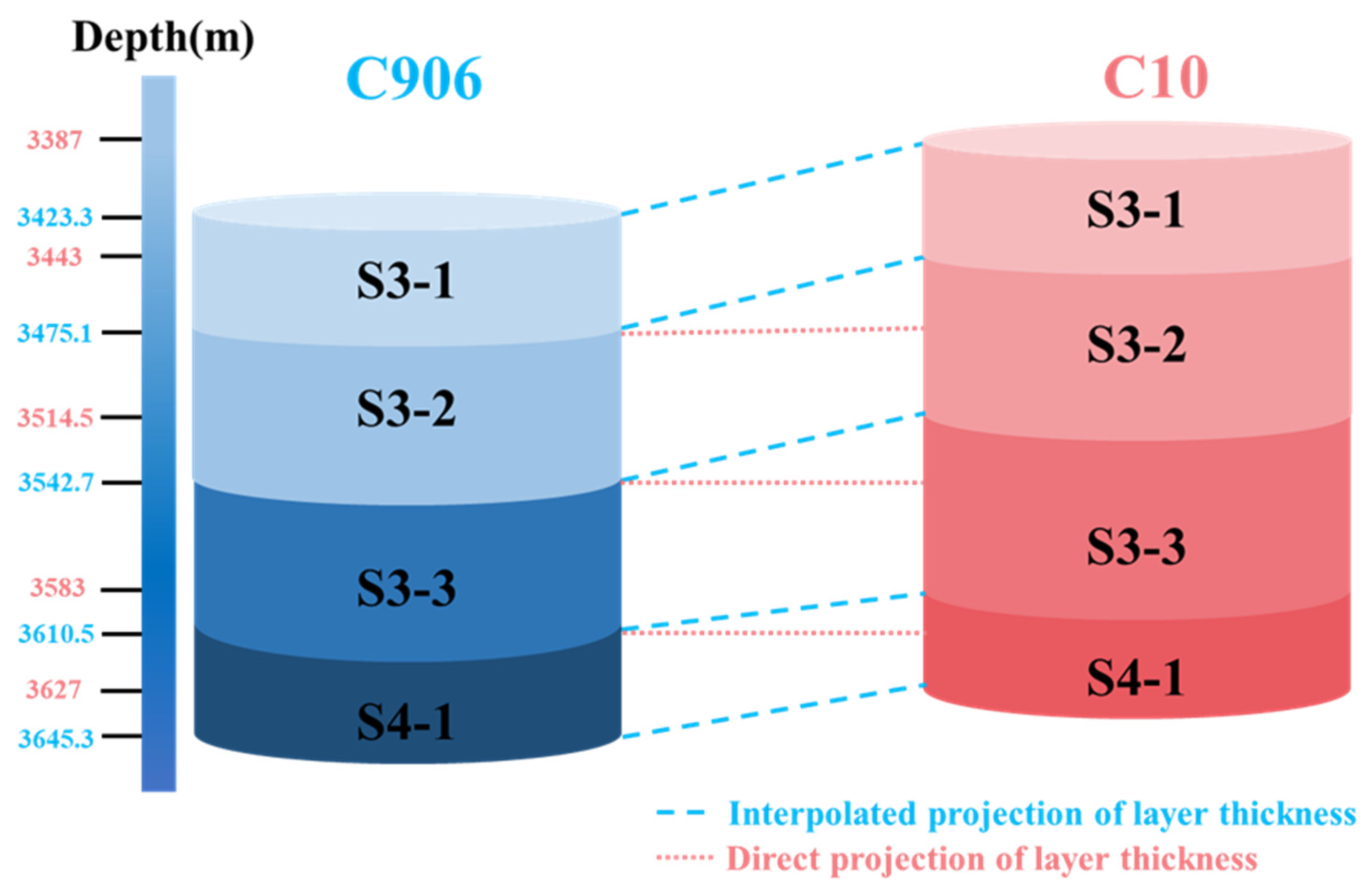Figure 5 illustrates the depth distribution of geological stratification between well C906 (offset well) and well C10 (target well). In conventional methods, when calculating sonic logging data for the S3-2 formation (3443 m–3514.5 m) in well C10, direct depth alignment is employed, where the sonic logging data actually utilizes the lower portion of the S3-1 formation (3423.3 m–3475.1 m) and the upper portion of the S3-2 formation (3475.1 m–3542.7 m) from well C906. Due to the different lithological and geological conditions between the two wells, this method exhibits low accuracy in subsequent calculations of rock mechanical parameters and mud weight windows using rock mechanics methods.

The geological sequence-matching method assumes that identical formations in offset wells within the same block possess uniform overall properties and vary uniformly within each layer, with the formation boundaries of the target well having been delineated through seismic data and historical drilling data during preliminary seismic exploration. This study utilizes well C906 to distribute post-drilling sonic logging data to each formation of well C10 through the geological sequence-matching method, as illustrated in Figure 5. For example, well C906 contains 1310 data points in the S3-1 formation (formation thickness: 51.8 m), and these 1310 data points are uniformly interpolated and distributed to the S3-1 formation of well C10 (formation thickness: 56 m). The depth calculation formula for the $i$ data point in the $j$ formation of the target well is shown in Equation (18) [29].

$$D{\mathrm{epth}}_{\mathrm{match}}=i·{\displaystyle \frac{D_{j+1}-D_j}{X}}+D_j$$

(18)

where ${Depth}_{match}$ represents the depth of the $i$ point in a specific stratigraphic layer of the target well; $D_{j+1}$ denotes the depth of the bottom boundary of a specific stratigraphic layer in the target well; $D_j$ represents the depth of the top boundary of a specific stratigraphic layer in the target well; and X is the number of post-drilling sonic logging data points in a specific stratigraphic layer of the offset well.

The data from well C906 processed using the geological sequence-matching method is designated well C10_match. The variation of selected parameters with depth for wells C906, C10, and C10_match is presented in Figure 6. It is evident that the C10_match well data processed through the geological sequence-matching method exhibits fundamentally identical trends to well C10, with consistent variations in detailed characteristics, although certain differences in data values persist. Compared to the conventional depth-based alignment method for processing C906 well data, the geological sequence-matching method, while unable to achieve complete consistency between offset well data and target well data, enables the predicted data trends to more closely approximate actual conditions.

3. Physics Model-Guided Deep Learning Prediction Method and Model Development for Mud Weight Window

3.1. Feature Engineering and Correlation Analysis

This study establishes its data foundation using logging data acquired from the field. Given that abnormal values (identified as −999.99) exist in the initial and terminal segments of logging data acquisition, along with occasional occurrences of such anomalies in intermediate sections, abnormal values at both ends are removed and depth calibration operations are completed. For intermediate abnormal values, identification is performed using the 3-sigma criterion, followed by replacement through linear interpolation of offset data points. For offset wells with relatively scarce measured data of Pp, Pm, and Pf, calculations are conducted using the aforementioned conventional rock mechanics methods based on post-drilling logging data. Subsequently, the calculated pressure profiles are calibrated against measured values to serve as reference standards. This study utilizes data from the C oil field, encompassing measured formation pressure values across multiple depth intervals. Comparative analysis reveals excellent consistency between the calculated results based on measured data and the three-pressure data from the C oil field, thereby validating the reliability of the proposed methodology.

It should be noted that the calculation parameters employed in this study are derived from years of drilling experience accumulated in the C oil field, forming a comprehensive empirical parameter system rather than a refined three-pressure profile constructed through detailed modeling. Additionally, all coefficients of the calculation parameters maintain consistency within the block boundaries. Furthermore, the calculated results align well with the actual drilling fluid density windows implemented in individual wells.

In this method, the ZDEN parameter (unit: g/cm³) has a numerical range of [2.5, 2.9], while the depth parameter (unit: m) extends to a numerical range of [2000, 4500]. Direct input of raw data into machine learning models would easily result in large-scale numerical dominance over small-scale values due to excessive differences in numerical magnitudes. To mitigate the adverse effects of data scale, feature dimensionality, and distribution differences on model performance, this study employs the max–min normalization method shown in Equation (19) to preprocess the dataset [30].

$$x^{\prime }={\displaystyle \frac{x-\min (x)}{\max \left(x\right)-\min \left(x\right)}}$$

(19)

where $x$ represents a feature dataset, $x^{\prime }$ denotes the transformed data, and max and min represent the maximum and minimum values of the dataset, respectively.

Correlation analysis can effectively quantify the strength of associations among multiple variables, thereby revealing the intrinsic relationships within data. This study employs the Spearman correlation coefficient to analyze the relationships between the statistically obtained parameters and the mud weight window. The calculation of the Spearman correlation coefficient is based on the original positions and re-ranked positions of the data [31,32], with specific calculation steps as follows.

(a)

Record the initial position $i$ of each data point in groups $x$ and $y$.

(b)

Sort the data into groups $x$ and $y,$ separately, according to specific sorting rules, and record the ranking positions $rg\left(x_i\right)$ and $rg\left(y_i\right)$ for each data point in both groups, which represent the ranks.

(c)

The difference between the rankings of the two data points in the $i$ pair is recorded as $d_i$, as shown in the following equation:

$$d_i=\mathrm{rg}\left(x_i\right)-\mathrm{rg}\left(y_i\right)$$

(20)

(d)

The Spearman correlation coefficient for groups $x$ and $y$ is calculated using the following formula:

$${\rho }_{i,\mathrm{Spearman}}=1-{\displaystyle \frac{6{\displaystyle \sum _{i=1}^n{d}_i^2}}{n\left(n^2-1\right)}}$$

(21)

The Spearman correlations between parameters are shown in Figure 7. The eccentricity of elliptical shapes reflects the strength of correlation between two parameters. The closer the ellipse approaches a circle, the weaker the correlation between parameters; the flatter the ellipse, the stronger the correlation between parameters. The orientation of the ellipse indicates whether the correlation between the two parameters is positive or negative. Additionally, the correlation strength between parameters can be identified through color gradient variations. Based on physical theory and Spearman correlation analysis, the relationships between Ed and Es, Ud and Us, St and Sc, C and J, and σ_h and σ_H originate from simple calculations using empirical formulas, exhibiting very high correlations. When selecting parameters, choosing one from each pair can reduce model complexity and computational requirements. It is noteworthy that Rd and Rs exhibit low correlations with the mud weight window, as these parameters are not utilized in traditional rock mechanics calculations. However, from a physical perspective, Rd and Rs can characterize lithological variations to some extent and may have localized influence on the mud weight window. Therefore, this study selects nine parameters for the model: Depth, DT, GR, ZDEN, Rd, Rs, Pp, Pm, and Pf, where the three parameters Pp, Pm, and Pf constitute the mud weight window.

3.2. Physics Model-Guided Deep Learning Prediction Method for Mud Weight Window

Traditional physics-based methods calculate rock mechanical parameters progressively through rock mechanics theory and empirical formulas; however, the dimensionless coefficients involved exhibit significant regional and depth-dependent characteristics, limiting prediction accuracy. While deep learning algorithms can establish complex nonlinear mapping relationships, they lack physical constraints and interpretability. Building upon the integration of traditional rock mechanics theory and deep learning techniques, this study proposes a physics-driven long short-term memory neural network (PD-LSTM) prediction method to enhance both the accuracy and interpretability of mud weight window predictions. Traditional physical models calculate various rock mechanical parameters through rock mechanics formulas, but the dimensionless coefficients and weighting factors involved often depend on regional and burial depth geological conditions, exhibiting significant non-uniqueness and regional adaptability limitations that make it difficult to comprehensively adapt to complex and variable wellsite environments. Although deep learning models possess powerful nonlinear mapping capabilities and can automatically learn complex high-order relationships between features, their “black box” characteristics result in a lack of necessary physical interpretation and domain credibility [33,34]. As shown in Figure 8, this study designs a physics-guided deep neural network architecture that embeds rock mechanics physical prior knowledge into the model, guiding deep learning to learn optimal mapping relationships within the space conforming to geological physical laws, thereby enhancing model performance stability and generalizability.

Specifically, a physics-driven layer is introduced into the model, utilizing key intermediate physical quantities from rock mechanics theory as the feature foundation to construct unified physical characterization variables. Based on correlation analysis results, six physical parameters are selected: VSH, Es, Us, St, J, and σ_H. Physical feature characterization is constructed through the following weighted relationship:

$$P\mathrm{hy}=a_1\cdot VSH+a_2\cdot Es+a_3\cdot Us+a_4\cdot St+a_5\cdot J+a_6\cdot {\sigma }_H$$

(22)

where $a_1$ through $a_6$ are trainable model parameters that are automatically optimized through backpropagation during the training process, preserving the computational logic of physical models while endowing the model with adaptive adjustment capabilities under different geological conditions. This physics-driven layer is implemented through custom neural network layers in TensorFlow, utilizing tensor operations to dynamically complete weighted summation calculations of various physical parameters, ensuring rigorous integration of physical processes with data-driven learning.

The drilling engineering process exhibits typical depth sequence characteristics: ① drilling operations are strictly conducted following well depth progression, with formation parameters displaying continuity and dependency in vertical profiles; ② formation sedimentation and evolution processes possess temporal cumulative effects, where deep structures are significantly influenced by shallow structures in their formation mechanisms. Therefore, this study adopts long short-term memory (LSTM) neural network modeling technology in the overall architecture to effectively capture long-range dependency information in well depth sequences through recurrent neural units [16,35]. The overall model input data is constructed using a fixed-length sliding window approach, where each training sample contains feature information from the previous 10 depth intervals (lookback = 10), enabling the model to fully utilize comprehensive information from historical well intervals for dynamic correction during current depth prediction, thereby enhancing prediction coherence and rationality.

In model design, the LSTM network first encodes time series data to extract dynamic evolution features [36,37]; subsequently, the physics-driven layer calculates physical feature representations based on static physical parameters at the current depth. These two components are concatenated through a feature fusion layer (concatenate) and then input into fully connected hidden layers (dense) to further learn deep-level combinatorial features, ultimately outputting target mud weight window values through a Tanh activation function [38]. To prevent model overfitting, dropout mechanisms are incorporated during the training process and combined with L1/L2 regularization to balance model complexity. The Adam optimization algorithm is employed to enhance training convergence speed and stability [39,40]. Upon completion of model training, the optimal weights of physical parameters within the physics-driven layer are simultaneously obtained, which can be further utilized for interpretative analysis of the weight of the influence of rock mechanical parameters on the mud weight window. The final model’s performance on both the test dataset and actual wellbore section predictions demonstrates that this physics-driven long short-term memory neural network can effectively integrate temporal information and the physical mechanisms of drilling formations, thereby significantly improving prediction accuracy and engineering application value.

3.3. Hyperparameter Tuning and Evaluation Metrics

Hyperparameters are critical configuration parameters that are preset before model training, and their combinations directly influence model performance; therefore, hyperparameter optimization constitutes a necessary step for achieving optimal prediction. This study employed L1/L2 regularization [41,42] and dropout techniques to constrain model complexity and constructed a search space encompassing the number of LSTM layer units, number of dense layer units, dropout rate, regularization strength, activation function, number of epochs, and batch size. Using the Randomized Search CV module from scikit-learn, with negative mean squared error as the objective function, 50 random sampling optimizations were performed based on the dataset excluding well C10_match. Through analysis of the hyperparameter space plot (Figure 9), the optimal parameter combination was determined, with both the validation and training sets achieving satisfactory convergence without underfitting or overfitting phenomena.

After establishing the optimal model, it is essential to quantify model performance and evaluate the discrepancies between predicted and true values, which constitutes the most direct approach for comparing the merits of various methods. This study employed four evaluation metrics: mean absolute error (MAE), root mean squared error (RMSE), mean absolute percentage error (MAPE), and coefficient of determination (R²) [43].

$$MAE={\displaystyle \frac{1}{n}}{\displaystyle \sum _{k=1}^n\left|y_{\mathrm{t}k}-y_{pk}\right|}$$

(23)

$$RMSE=\sqrt{{\displaystyle \frac{1}{n}}{\displaystyle \sum _{k=1}^n{\left(y_{tk}-y_{pk}\right)}^2}}$$

(24)

$$MAPE={\displaystyle \frac{1}{n}}{\displaystyle \sum _{k=1}^n\left|\frac{y_{\mathrm{t}k}-y_{pk}}{y_{tk}}\right|}$$

(25)

$$R^2=1-{\displaystyle \frac{{\displaystyle \sum _{k=1}^{\mathrm{n}}{(y_{pk}-y_{tk})}^2}}{{\displaystyle \sum _{k=1}^{\mathrm{n}}{(y_{tk}-\overline{y})}^2}}}$$

(26)

where $y_{tk}$ represents the true value of the sample at the $k$ point; $y_{pk}$ denotes the predicted value of the sample at the $k$ point; $\overline{y}$ is the mean of the true sample values; and $n$ represents the total number of samples.

4. Results and Discussion

4.1. Results

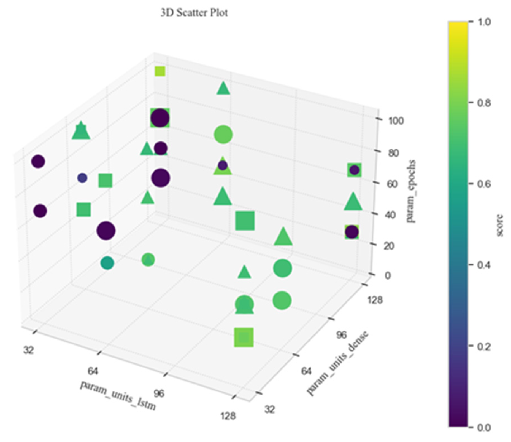
To validate the effectiveness of the proposed method, this study compared the prediction results of the proposed physics-guided prediction approach with those of traditional methods. In the traditional approach, the Bowers method was employed to calculate formation Pp consistent with the unloading curve, and Pm and Pf were computed using conventional rock mechanics formulas. In the physics-guided prediction method, all historical wells except well C10 were utilized, incorporating depth, DT, GR, ZDEN, Rd, Rs, and their regressed Pp, Pm, and Pf values for model learning and training. The hyperparameters of the theoretical layer for the proposed physics-guided LSTM neural network model, established through the random parameter search described in Section 3.3, are presented in

Table 1. Hyperparameter configuration of the physics-guided LSTM neural network model.

Hyperparameter		Units LSTM	Units Dense	Dropout Rate	L1_reg	L2_reg	Activation	Batch Size	Epochs
Methods
Physics-driven layer machine learning method	Pp	32	128	0.4	0.001	0.001	‘relu’	128	70
	Pm	32	64	0.4	0.1	0.001	‘relu’	128	50
	Pf	64	32	0.2	0.1	0.001	‘relu’	32	70

. Through the hyperparameter configuration of the theoretical layer approach, regarding the dense layer unit configuration, Pp prediction employed the largest dense layer with 128 units, while Pm and Pf utilized 64 and 32 units, respectively, indicating that formation pore pressure requires more complex nonlinear mapping relationships. In terms of regularization coefficients, pore pressure adopted a smaller L1 regularization coefficient of 0.001, whereas collapse pressure and fracture pressure employed a larger L1 regularization coefficient of 0.1, while all tasks utilized large L2 regularization coefficients to maintain consistency in weight constraints.

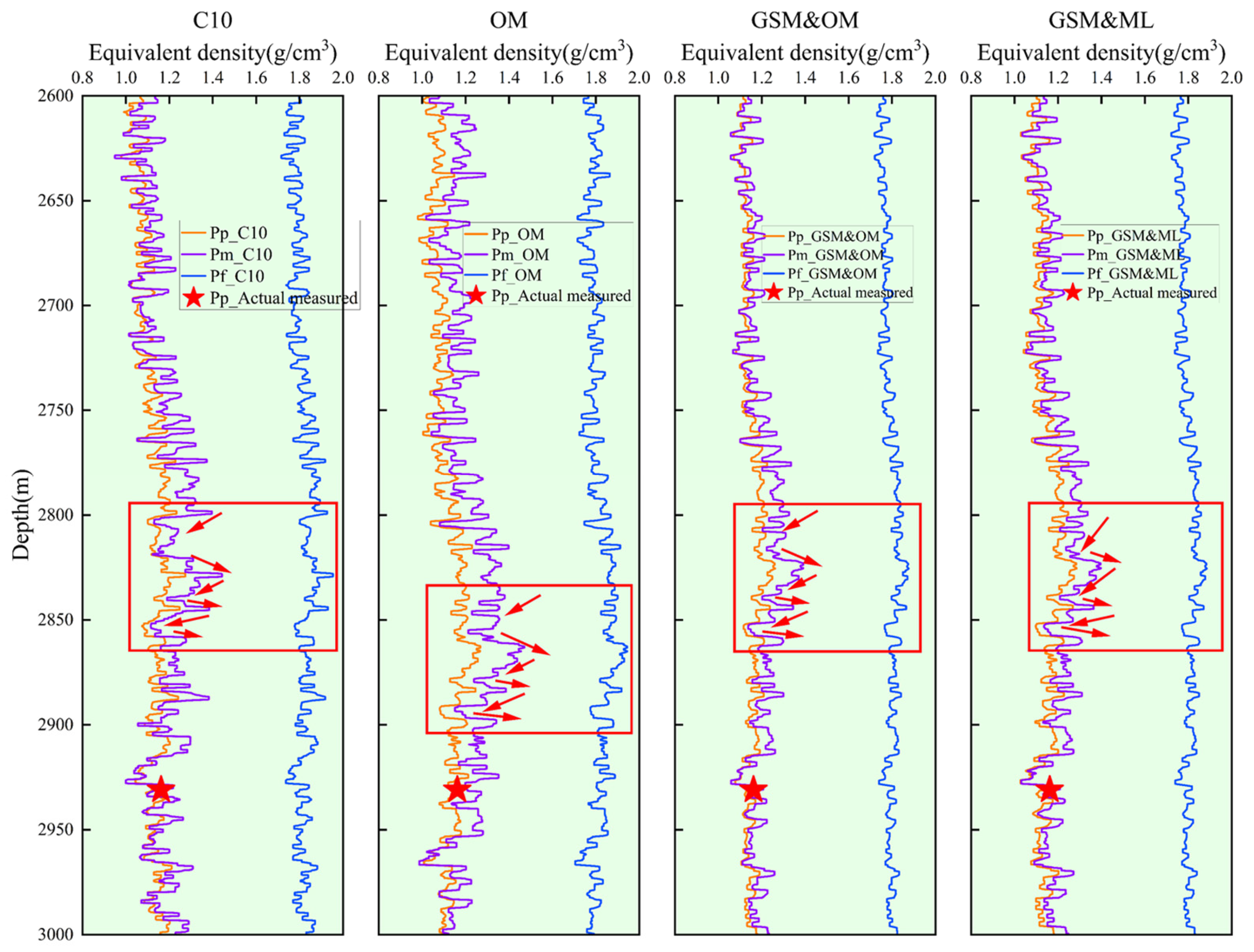
The mud weight window prediction results from the three methods and the post-drilling regression results of well C10 are presented in Figure 10. It can be clearly observed that the predicted results from all three methods are generally consistent with the numerical magnitude and trends of well C10. The red box in the figure highlights a section where distinct trend variations can be observed. Taking pore pressure as an example, within this wellbore interval, Pp initially exhibits a slight decreasing trend, followed by relative stability, then a slight increasing trend, which is immediately followed by a decreasing trend, an increasing trend, another decreasing trend, and subsequently a rapid increasing trend. However, the depth window where the Pp_Original method (Pp_OM, the following text uses abbreviations) exhibits this trend pattern occurs from 2840 m to 2900 m, while the trend windows for both the Pp_ GSM&Original method (Pp_GSM&OM, the following text uses abbreviations) and Pp_GSM&Machine learning (Pp_GSM&ML, the following text uses abbreviations) range from 2799 m to 2860 m, which is consistent with the trend window found by the post-drilling regression analysis of well C10. It is noteworthy that this trend is consistent with the results observed in DT, ZDEN, GR, and Rs presented in Figure 6. The underlying reason for this is that the original method neglects inter-well geological variations when predicting mud weight windows. After GSM processing, the geological conditions of the target well can be estimated with maximum precision in situations where subsurface data cannot be directly obtained. This depth alignment capability, through accurate capture of local dynamic variation characteristics of mud weight windows in complex formations, enables meter-scale refined customization of mud weight window schemes under complex formation conditions, thereby providing more robust technical support for pre-drilling engineering design.

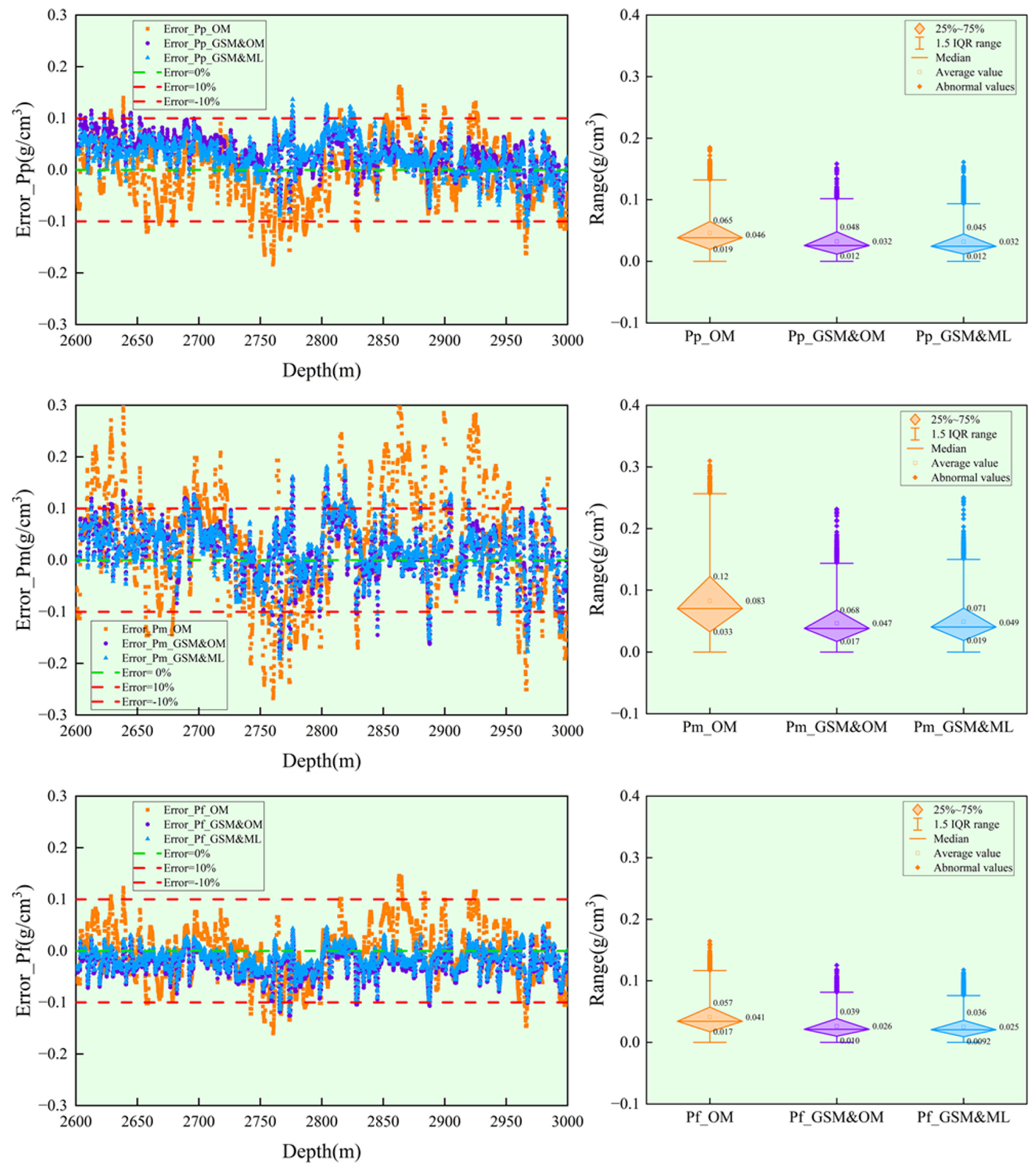
Figure 11 presents the box plots of error and absolute error distributions for Pp, Pm, and Pf predicted by the three methods. From the perspective of error distribution trends, the methods utilizing GSM processing as geological parameters demonstrate that the errors of Pp, Pm, and Pf are all distributed within ±10%. Regarding collapse pressure errors, the absolute error mean of Pm_OM is 0.083 g/cm³, while the error means of Pm_GSM&OM and Pm_GSM&ML are as low as 0.047 and 0.049 g/cm³, respectively. The error means of Pm_GSM&OM and Pm_GSM&ML represent a decrease of 43.37% and 40.96% compared to the original method, respectively, demonstrating the effectiveness of the proposed approach in this study. Regarding pore pressure errors, the error mean of Pp_OM is 0.046 g/cm³, while the error means of both Pp_GSM&OM and Pp_GSM&ML are as low as 0.032 g/cm³. The error means of Pp_GSM&OM and Pp_GSM&ML show a decrease of 30.43% compared to the original method. In terms of fracture pressure errors, the error mean of Pf_OM is 0.041 g/cm³, while the error means of Pf_GSM&OM and Pf_GSM&ML are as low as 0.026 and 0.025 g/cm³, respectively. The error means of Pf_GSM&OM and Pf_GSM&ML are decreased by 36.59% and 39.02% compared to the original method, respectively. These results demonstrate the effectiveness of the approach proposed in this study.

Evaluation metrics were calculated for the predicted values obtained from the three methods and the actual values from post-drilling regression of well C10, yielding

Table 2. Performance evaluation of three methods.

	Pp_OM	Pp_GSM&OM	Pp_GSM&ML	Pm_OM	Pm_GSM&OM	Pm_GSM&ML	Pf_OM	Pf_GSM&OM	Pf_GSM&ML
MAE	0.048	0.038	0.035	0.087	0.046	0.045	0.043	0.029	0.025
RMSE	0.060	0.046	0.043	0.11	0.057	0.057	0.053	0.036	0.032
MAPE	4.30	3.51	3.14	7.51	3.93	3.862	2.366	1.585	1.361
R2	−0.21	0.29	0.39	−0.47	0.60	0.60	−0.614	0.247	0.414

, which presents the performance evaluation of the three methods. According to the calculation results, all three methods can predict mud weight windows to a certain extent. Following the evaluation criteria, the method with the highest metric scores is highlighted (bold and underlined in the table). The proposed theoretical layer model demonstrates the best performance across all metrics. This is consistent with the results from direct observation in Figure 10 and error analysis in Figure 11. It is worth noting that during performance evaluation of the traditional method, an anomalous situation occurred where $R^2$ values were negative. This indicates that the traditional method exhibits extremely poor fitting performance when using logging data from well C906 to predict the mud weight window of well C10. This indirectly reflects that the proposed method effectively improves the fine prediction of mud weight windows.

4.2. Limitations

Although the physics-guided deep learning method for mud weight window prediction proposed in this study demonstrates significant advantages in case validation, several limitations and areas for improvement remain in the following aspects.

The predictive accuracy of the proposed method is heavily dependent on the quality and quantity of historical data. In practical engineering applications, obtaining large amounts of continuous formation pressure ground truth data is challenging due to the high costs associated with direct measurement techniques such as Repeat Formation Tester (RFT) and Modular Dynamic Tester (MDT). The “true values” values utilized in this study are actually estimates derived from post-drilling logging data and drilling records through traditional rock mechanics regression calibration methods, rather than absolute true formation conditions. This limitation in data acquisition methodology may adversely affect model training effectiveness and restrict the method’s applicability in data-scarce regions.

Meanwhile, the discussion of data quality dependence in this paper remains primarily at the qualitative descriptive level. Future work should consider establishing a relationship model between data quality and prediction accuracy. By designing datasets with different noise levels (e.g., 5%, 10%, 15%, 20% random errors), the trend of prediction error variation with data quality degradation can be systematically analyzed, and acceptable data quality thresholds can be provided. Furthermore, minimum dataset requirements need to be quantified by progressively reducing the number of training samples. Additionally, a data integrity assessment framework should be established to analyze the differential impacts of missing logging parameters on various pressure predictions (pore pressure, collapse pressure, and fracture pressure), thus providing guidance for data collection strategies in practical engineering applications.

Although this study embeds traditional rock mechanics theory into the deep learning framework through physics-driven layers, inherent contradictions between the two approaches persist. Physical models, based on simplified assumptions and empirical coefficients, may introduce systematic errors under complex geological conditions, while traditional machine learning models typically function as “black boxes” with poor interpretability and lack of intuitive understanding [44]. Occasionally, machine learning models may generate parameter combinations that violate physical laws during optimization processes. How to fully leverage the nonlinear mapping capabilities of machine learning while ensuring physical reasonableness remains a theoretical issue requiring in-depth exploration.

Despite the introduction of physics-driven layers, the “black box” characteristics of deep learning models persist, particularly in the temporal processing mechanisms of LSTM networks, where it is difficult to intuitively understand how the model weighs geological information from different depth intervals. Furthermore, the model’s generalization capability across different geological environments and structural backgrounds requires further verification, especially for new blocks with geological characteristics significantly different from the training data.

The GSM method assumes that identical formations between adjacent wells and target wells possess similar geological characteristics. However, in areas with complex structures and strong lateral heterogeneity, this assumption may not hold. Geological factors such as fault development, lithofacies changes, and sedimentary environment variations may lead to significant deviations in formation matching results, thereby affecting final prediction accuracy.

To address the aforementioned limitations, future research should focus on improvements in the following aspects: (1) integrating multi-source information including seismic data and geological modeling to construct a more comprehensive geological constraint system; (2) developing physics-constrained regularization techniques to ensure the physical reasonableness of model predictions; (3) establishing adaptive model selection mechanisms for different geological types; and (4) conducting model interpretability analysis. For instance, for the interpretation of parameters’ importance, the SHAP method can be employed to quantify the contribution of each input parameter to prediction results; for engineering decision support interpretation, prediction uncertainty can be transformed into risk assessment indicators to provide refined safety threshold recommendations for mud density design, thereby enhancing the credibility and engineering applicability of prediction results.

5. Conclusions

This study addresses the problem of insufficient accuracy in traditional mud weight window prediction methods under complex geological conditions and proposes a physics-guided deep learning prediction method for mud weight windows. This method integrates physical models and deep learning models, enabling fine prediction of mud weight windows prior to drilling operations, thereby providing effective support for reducing downhole complications and facilitating more detailed design of wellbore structure, drilling fluids, cementing operations, and field emergency response plans. The effectiveness of the proposed method was validated through a practical case study in Block C of an oilfield in Northwest China.

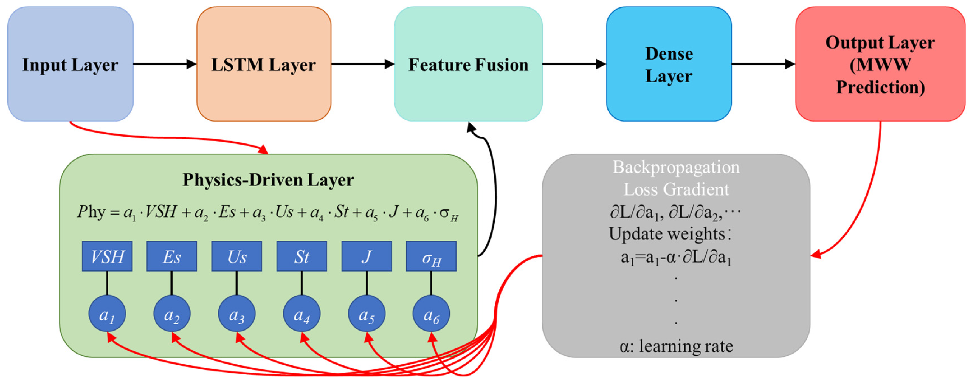
① An LSTM neural network architecture embedded with a physics-driven layer was constructed, achieving deep integration of traditional rock mechanics theory with deep learning algorithms. Through the comprehensive characterization of intermediate variables including VSH, Es, Us, St, J, and σ_H, this method maintains the interpretability of physical models while fully exploiting the advantages of machine learning in handling complex nonlinear relationships.

② GSM processing was validated to achieve precise alignment of geological feature trends in the depth dimension, establishing a foundation for meter-scale fine prediction prior to drilling. Taking pore pressure in the case study as an example, the specific trend variation window predicted by the traditional method was located in the 2840 m–2900 m depth interval, while the predicted specific trend window after GSM processing was accurately aligned to 2799 m–2860 m, which is completely consistent with the actual geological conditions of the target well. This depth alignment capability enables accurate capture of local variation characteristics of mud weight windows in complex formations, achieving meter-scale refined customization of mud weight window schemes for complex formations and providing more reliable technical support for pre-drilling engineering design.

③ Case validation results demonstrate that the proposed method exhibits significant advantages in predicting pore pressure, collapse pressure, and fracture pressure. Compared to traditional methods, collapse pressure prediction error was reduced by 40.96%, pore pressure prediction error was reduced by 30.43%, and fracture pressure prediction error was reduced by 39.02%. All evaluation metrics outperformed both traditional methods and the purely GSM-based approach.

This study enables fine prediction of mud weight windows prior to drilling operations, providing effective technical support for wellbore structure design, drilling fluid scheme optimization, cementing scheme formulation, and field emergency plan preparation. It demonstrates significant engineering application value for reducing downhole complications and improving drilling efficiency. Effective validation in drilling engineering indicates that this processing approach may possess similar potential in other geological engineering problems, including reservoir parameter prediction, geological hazard assessment, and groundwater resource evaluation.