Operational Temperature Optimization in Hydrogen Turbine Blades via Time-Fractional Conformable Sensitivity Analysis

Abstract

This study focuses on optimizing the thermal performance of hydrogen turbine blades through a sensitivity analysis using generalized fractional calculus. The approach is designed to capture the transient temperature dynamics and optimize thermal profiles by analyzing the influence of a fractional-order parameter on the system’s behavior. The model was implemented in Python, using Monte Carlo simulations to evaluate the impact of the parameter on the temperature evolution in different thermal regimes. Three distinct regions were identified: the Quasi-Uniform Region (where fractional effects are negligible), the Sub-Classical Region (characterized by delayed thermal behavior), and the Super-Classical Region (exhibiting enhanced heat accumulation). Regression analyses reveal quadratic and cubic dependencies of blade temperature on the fractional-order parameter, confirming the robustness of the model with R² values greater than 0.96. The study highlights the potential of using fractional calculus to optimize the thermal response of turbine blades, helping to identify the most suitable parameters for faster stabilization and efficient heat management in hydrogen turbines. Furthermore, it was found that by adjusting the fractional-order parameter, the system can be optimized to reach equilibrium more rapidly while achieving higher temperatures. Importantly, the equilibrium is not altered but rather accelerated based on the chosen parameter, ensuring a more efficient thermal stabilization process.

1. Introduction

The global transition toward carbon-neutral energy systems has catalyzed significant advancements in both renewable energy technologies and the associated supporting infrastructure [1]. Within this transformative landscape, hydrogen energy has emerged as a pivotal clean energy vector, with hydrogen-fueled turbines constituting a critical technological solution for efficient energy conversion [2]. Achieving optimal operational performance in such systems necessitates the development and application of sophisticated mathematical frameworks capable of accurately capturing the underlying thermo-fluid dynamics.

Mathematical modeling, therefore, plays an indispensable role in deciphering the intricate physical phenomena that govern hydrogen turbine performance. Among the most critical aspects is the thermal management of turbine blades, where even marginal enhancements in efficiency can lead to substantial energy savings and significant reductions in emissions [3]. In this context, sensitivity analysis becomes paramount, offering a rigorous methodology to evaluate how parametric variations influence system behavior. This is particularly relevant in fractional-order models, where the non-local properties of the derivatives introduce unique challenges in exploring the parameter space.

Recent advancements in hydrogen gas turbine technology have garnered significant attention, driven by the growing need for cleaner, more sustainable energy sources. Hydrogen’s potential as a fuel for gas turbines is particularly promising, offering zero CO₂ emissions and high energy density [4]. However, challenges persist in hydrogen combustion characteristics, such as combustion stability and material compatibility, which complicate its widespread adoption [4]. Moreover, the limited availability of green hydrogen and the high production costs raise concerns about the feasibility of a rapid transition to hydrogen-powered systems, especially in aviation applications [5]. Despite these obstacles, research continues to focus on overcoming these barriers by improving combustion technologies, such as micro-mix lean combustion and staged combustion, and enhancing hydrogen production technologies [5]. Additionally, the incorporation of hydrogen-powered gas turbines in terrestrial and aerospace applications has shown promise, although significant progress is still needed in terms of infrastructure and technological innovation [6]. This study aims to contribute to this ongoing effort by exploring the optimization of hydrogen turbine blades, with a particular focus on thermal management through time-fractional conformable sensitivity analysis.

This work presents a comprehensive sensitivity analysis of a fractional-order thermal model for hydrogen turbine blades, grounded in the conformable calculus framework established in [7]. While the fundamental properties of conformable derivatives were rigorously characterized in [8], our study extends these developments by addressing their implementation for thermal optimization in hydrogen turbines—a technology increasingly central to the global energy transition [2]. The primary objective is to examine how the fractional-order parameter, denoted by $\alpha \in (0,1]$, influences the spatiotemporal temperature distribution along turbine blades. Ultimately, the objective is to determine the theoretically optimal value of $\alpha$ that maximizes thermal performance, achieving a balance between efficiency enhancements and material limitations.

This parameter optimization is particularly vital for hydrogen turbines, where blade temperature control directly impacts energy conversion efficiency and component durability. By establishing the functional relationship between $\alpha$ and the thermal behavior, this work enables targeted optimization of time-fractional conformable systems—representing a novel contribution to turbine performance enhancement. Beyond identifying optimal $\alpha$ values, the analysis also characterizes their sensitivity under different operating regimes, thereby offering actionable insights for industrial implementation.

The modeling approach leverages generalized conformable derivatives, which confer distinct advantages over classical integer-order and conventional fractional operators. As demonstrated in [3], achieving accurate thermal characterization in turbine systems remains challenging due to complex boundary conditions and transient operational regimes. Our conformable framework effectively addresses these challenges by ensuring dimensional consistency and adapting to system variations through the conformable function $\psi (t,\alpha )$.

Fractional calculus has shown particular promise in capturing the non-local and memory-dependent dynamics that typify turbine blade thermal behavior. The generalized model developed in [7] laid the theoretical groundwork for employing these methods in hydrogen turbines. Building on this foundation, the present study introduces a rigorous fractional-order $\alpha$ sensitivity analysis, providing critical insights for temperature regulation optimization strategies, an increasingly important consideration in clean hydrogen systems, as emphasized by [2].

The optimization perspective is especially compelling in light of the model’s proven ability to replicate realistic thermal anomalies, as previously demonstrated in [7]. Through strategic modulation of $\alpha$, the framework reproduces behaviors that are analogous to those observed experimentally [9], positioning this parameter as an anomalous coupling coefficient that governs energy and mass transfer. Our simulations highlight how conformable derivatives inherently capture complex stabilization dynamics in turbine blades, providing a robust mathematical foundation for performance optimization.

The sensitivity analysis methodology employed in this study adapts the Monte Carlo techniques pioneered by [10,11], specifically tailored to assess the influence of $\alpha$ on temperature evolution in hydrogen turbine blades. Implemented using Python’s scientific computing ecosystem [12], this numerical framework facilitates efficient solution of conformable differential equations while enabling a statistically sound exploration of parameter sensitivity across various operational conditions.

When benchmarked against alternative fractional modeling approaches, conformable derivatives offer notable computational efficiencies and enhanced physical interpretability—attributes that are particularly advantageous for engineering applications. Nonetheless, certain theoretical limitations remain regarding the incorporation of memory effects and stochastic variability, highlighting avenues for future investigation. Expanding on the framework proposed in [7], this study demonstrates the utility of conformable derivative-based sensitivity analysis to systematically optimize the operation of hydrogen turbines, thus contributing to the development of more efficient and resilient clean energy systems, as envisioned in [1,2].

The remainder of this paper is organized as follows. Section 2 introduces the mathematical foundations of conformable calculus, establishing the theoretical framework employed throughout this investigation. Section 3 presents the thermal modeling approach and optimization methodology; the modeling assumptions are outlined in Section 3.1, followed by a comprehensive description of the sensitivity analysis technique in Section 3.2. Section 4 presents the Results and Comparative Analysis of Thermal Regimes, subdivided into three distinct dynamical regimes: Section 4.1, Section 4.2 and Section 4.3 provide rigorous examination of the system’s behavior, with particular emphasis on thermal dynamics governed by the fractional parameter $\alpha$. Section 5 synthesizes these findings into a systematic framework for optimal fractional parameter selection to enhance thermal management in hydrogen turbines. Section 6 evaluates these results within the context of practical turbine design considerations. Finally, Section 7 summarizes the key findings and proposes future research directions in fractional-order modeling for advanced energy systems.

2. Foundations and Basic Concepts of the Conformable Derivative

This section presents the theoretical foundations and preliminary concepts related to the conformable derivative. Its formal definition, fundamental properties, and the manner in which it extends classical derivative concepts are examined. A thorough understanding of these elements is essential for the appropriate application of the conformable derivative in the modeling of hydrogen turbine blade dynamics.

As a contemporary development in fractional calculus, the conformable derivative was conceived to address certain shortcomings of traditional integer-order differentiation. Following Khalil et al.’s initial work [13], this operator provides a more versatile framework particularly suited for systems exhibiting memory effects and hereditary properties. Further developments by Gateaux led to the linear extended Gateaux derivative and the formalization of the generalized conformable derivative, as presented in [14].

Definition 1 

(Conformable function). A conformable function $\psi (t,\alpha )$ is a differentiable function in t that satisfies:

$$\begin{array}{cc}\hfill \psi (t,1)& =1,\hfill \\ \hfill \psi (t,\alpha )& \ne \psi (t,\beta ),when\alpha ,\beta \in (0,1],\hfill \\ \hfill \psi (t,\alpha )& \ne 0,forany\alpha \in (0,1].\hfill \end{array}$$

(1)

Definition 2 

(Generalized Conformable Derivative). For a conformable function $\psi (t,\alpha )$ and a differentiable function $f:\mathbb{R}\to \mathbb{R}$, the generalized conformable derivative of order α at t, denoted ${}^{\psi }D_t^{\alpha }f\left(t\right)$, extends classical differentiation by incorporating $\psi (t,\alpha )$ and is defined as:

$$\begin{array}{cc}\hfill {}^{\psi }D_t^{\alpha }f\left(t\right)& =\underset{\epsilon \to 0}{lim}{\displaystyle \frac{f(t+\epsilon \psi (t,\alpha \left)\right)-f\left(t\right)}{\epsilon }}.\hfill \end{array}$$

(2)

Here, $\alpha \in (0,1]$ determines the derivative’s scaling behavior. Applying L’Hôpital’s rule yields:

$$\begin{array}{cc}\hfill {}^{\psi }D_t^{\alpha }f\left(t\right)& =\psi (t,\alpha ){\displaystyle \frac{d}{dt}}f\left(t\right).\hfill \end{array}$$

(3)

Theorem 1  

(Properties of the Generalized Conformable Derivative). For α-differentiable functions $f,g$ on $A\subset \mathbb{R}$ with $\alpha \in (0,1]$, and real constants $a,b,c$, the following holds:

• ${}^{\psi }D_t^{\alpha }c=0$.
• ${}^{\psi }D_t^{\alpha }(af+bg)=a{}^{\psi }D_t^{\alpha }f+b{}^{\psi }D_t^{\alpha }g$.
• ${}^{\psi }D_t^{\alpha }\left(fg\right)=f{}^{\psi }D_t^{\alpha }g+g{}^{\psi }D_t^{\alpha }f$.
• ${}^{\psi }D_t^{\alpha }\left({\displaystyle \frac{f}{g}}\right)={\displaystyle \frac{g{}^{\psi }D_t^{\alpha }f-f{}^{\psi }D_t^{\alpha }g}{g^2}}$.
• ${}^{\psi }D_t^{\alpha }(f\circ g)=f^{\prime }\left(g\right){}^{\psi }D_t^{\alpha }g$.

See [15] for proofs.

Definition 3 

(Generalized Conformable Integral). For $a\ge 0$, $t\ge a$, and f defined on $(a,t]$, with conformable function $\psi (t,\alpha )$, the generalized α-conformable integral is:

$$\begin{array}{c}\hfill {}_a{}^{\psi }I_t^{\alpha }f\left(t\right)={\int }_a^t{\displaystyle \frac{f\left(\tau \right)}{\psi (\tau ,\alpha )}}d\tau .\end{array}$$

(4)

The operators ${}^{\psi }D_t^{\alpha }$ and ${}_a{}^{\psi }I_t^{\alpha }$ are inverse operations and satisfy fundamental calculus theorems as shown in [15].

Theorem 2 

(First Fundamental Theorem of Generalized Fractional Conformable Derivatives). For $a>0$, $t>a$, $\alpha \in (0,1]$, and continuous f:

$${}^{\psi }D_t^{\alpha }\left({}_a{}^{\psi }I_t^{\alpha }f\right)=f\left(t\right).$$

(5)

Theorem 3 

(Second Fundamental Theorem of Generalized Fractional Conformable Derivatives). For $a>0$, $t>a$, $\alpha \in (0,1]$, and differentiable f:

$${}_a{}^{\psi }I_t^{\alpha }\left({}^{\psi }D_t^{\alpha }f\right)=f\left(t\right)-f\left(a\right).$$

(6)

Model Description

The blade temperature is estimated following the approach in [7], assuming uniform heating and neglecting hot gas temperature variations due to limited geometric and cooling data [7,16,17,18]. The model used in this study is given by Equation (7):

$$\begin{array}{cc}\hfill {}^{\psi }D_t^{\alpha }{T}_{bl}& ={\displaystyle \frac{A{T}_{bl}+B}{C_{P_{bl}}\left(T_{bl}\right)}},T_{bl}\left(t_0\right)=T_{bl,0}.\hfill \end{array}$$

(7)

where:

$$\begin{array}{cc}\hfill A& ={\displaystyle \frac{h_{bl}{A}_{bl}-{\dot{m}}_{cl}{c}_{p_{cl}}\epsilon }{n_{bl}}},\hfill \\ \hfill B& ={\displaystyle \frac{h_{bl}{A}_{bl}{T}_g+{\dot{m}}_{cl}{c}_{p_{cl}}\epsilon T_{cl,1}}{n_{bl}}},\hfill \\ \hfill {\dot{m}}_{cl}& ={\displaystyle \frac{p_2{K}_1}{\sqrt{T_1}}}\sqrt{1-{\displaystyle \frac{p_2^{\prime }}{p_1}}},\hfill \end{array}$$

(8)

where $n_{bl}$ is the number of blades, $c_{p_{cl}}$ denotes the specific heat capacity of the blade cooling air, while $C_{P_{bl}}$ represents the specific heat capacity of the blade material, $A_{bl}$ the external surface area, $h_{bl}$ the heat transfer coefficient, $T_g$ the gas temperature, ${\dot{m}}_{cl}$ the coolant mass flow rate, and $\epsilon$ the heat transfer efficiency. $T_1$ and $p_1$ are evaluated at the coolant extraction point, while $p_2^{\prime }$ is the static pressure at the row exit.

For nozzle-cooled blades, $T_g$ corresponds to the absolute stagnation temperature; for rotor blades, it is the rotor-relative stagnation temperature. In film-cooled blades, $T_g$ is replaced by the adiabatic wall temperature [16,17,18], and $T_{cl,1}$ is the coolant temperature at the inlet of the blade’s internal cooling circuit, and $\epsilon$ is the heat transfer efficiency.

Remark 1. 

The coefficient B is always positive, while A may be positive or negative, affecting $T_{bl}$. If $A<0$, $T_{bl}$ decreases; if $A>0$, $T_{bl}$ increases, given $C_{P_{bl}}>0$.

The conformable function $\psi$ represents an anomalous heat transfer coefficient, while $\alpha$ denotes a temporal delay factor. The blade material is titanium, with molar heat capacity modeled as [19]:

$${\widehat{C}}_{P_{bl}}\left(T_{bl}\right)=37.27944+4.76976\times {10}^{-3}{T}_{bl}-{\displaystyle \frac{1811672}{T_{bl}^2}}\left[{\displaystyle \frac{\mathrm{J}}{\mathrm{mol}·\mathrm{K}}}\right].$$

(9)

Assuming a base of 1 mol of titanium (this assumption can be adjusted depending on the context), the heat capacity becomes:

$$C_{P_{bl}}\left(T_{bl}\right)={\widehat{C}}_{P_{bl}}\left(T_{bl}\right)\times \left(1\mathrm{mol}\mathrm{Ti}\right)=37.27944+4.76976\times {10}^{-3}{T}_{bl}-{\displaystyle \frac{1811672}{T_{bl}^2}}\left[{\displaystyle \frac{\mathrm{J}}{\mathrm{K}}}\right].$$

(10)

It was used two conformable functions, defined rigorously as follows:

$$\begin{array}{cc}\hfill {\psi }_1(t,\alpha )& =a^{b(1-\alpha )f\left(t\right)},\mathrm{defined}\mathrm{on}\left({\mathbb{R}}^{+}\cap \mathrm{Dom}\left(f\right)\right)\times (0,1],a\in {\mathbb{R}}^{+},b\in \mathbb{R},f\left(t\right)\in C^0\left(\mathbb{R}\right),\hfill \\ \hfill {\psi }_2(t,\alpha )& ={(\xi sin\left(\theta t\right)+1)}^{1-\alpha },\mathrm{defined}\mathrm{on}{\mathbb{R}}^{+}\times (0,1],0<\xi <1,\theta \in \mathbb{R},\hfill \end{array}$$

(11)

where $f\left(t\right)=sin\left(\theta t\right)$. The parameters used in the simulations are detailed in

Table 1. Parameters used in the simulations, their values, and units. The subscript cl refers to blade cooling air, bl denotes the blade material, and g indicates the working gas.

Parameter	Value	Units
a	e	Dimensionless
$\xi$	$0.99$	Dimensionless
b	$2.8$	Dimensionless
$f\left(t\right)$	$sin\left(\theta t\right)$	Dimensionless
$\theta$	$5\pi$	$1/s$
$h_{\mathrm{bl}}$	10.0	W/(m2·K)
$A_{\mathrm{bl}}$	5.0	m2
${\dot{m}}_{\mathrm{cl}}$	200	kg/s
$c_{p_{\mathrm{cl}}}$	1.0	J/(kg·K)
$\epsilon$	0.8	Dimensionless
$T_g$	500	K
$T_{{\mathrm{cl}}_1}$	300	K
$n_{\mathrm{bl}}$	1.0	Dimensionless
$\theta$	5$\pi$	1/s

, including their values and units.

Figure 1 shows the simulation results of blade temperature dynamics $T_{bl}$ for different values of $\alpha$ of $0.2,0.4,0.6,0.8$ and $1.0$, illustrating the variety of thermal behaviors that can arise.

3. Methods

This section outlines the methodology employed for the stabilized analysis. Initially, the region of interest is defined, with the study centered on a temperature range near $T_{bl}=450$ K.

To enhance the interpretation of the results, the time domain is partitioned into three distinct regions, each characterized by specific thermal behaviors corresponding to variations in the fractional derivative order, $\alpha$.

• Quasi-Uniform Region ($t\in [0.26,0.29]$ s): In this interval, all temperature curves are nearly identical, regardless of the value of $\alpha$. The temperature remains within the range of 450 to 467 K, showing minimal deviation from the classical model. ${\overline{t}}_{QUR}=0.275$
• Sub-Classical Region ($t\in [0.17,0.26]$ s): Before reaching the Quasi-Uniform Region, the temperature values obtained for $\alpha <1$ are consistently lower than those predicted by the classical model. This indicates a delayed temperature dynamics when using fractional derivatives.m the classical model. ${\overline{t}}_{sub}=0.215$
• Super-Classical Region ($t\in [0.29,0.4]$ s): After the Quasi-Uniform Region, the use of fractional derivative orders different from $\alpha =1$ results in temperature values exceeding those of the classical model. This suggests an enhancement in heat accumulation due to the fractional-order effects. ${\overline{t}}_{super}=0.35$

The study region encompasses both the Sub-Classical and Super-Classical regions, as these intervals highlight the influence of fractional-order derivatives on the temperature dynamics. The Quasi-Uniform Region serves as a reference point where fractional effects are minimal. Analyzing the deviations observed within the study region allows for a deeper understanding of the influence of the parameter $\alpha$ on the system’s thermal response.

It is important to highlight that the Super-Classical and Sub-Classical regions are the only relevant intervals for analysis. In contrast, the Quasi-Uniform Region exhibits identical behavior for all values of $\alpha$, making it uninformative for sensitivity analysis.

The invariance observed in the equilibrium region can be demonstrated analytically, as shown in the following analysis. By examining the conformable fractional differential equation and conducting an equilibrium assessment, the system can be reformulated as an ordinary differential equation:

$$\begin{array}{cc}\hfill {}^{\psi }D_t^{\alpha }{T}_{bl}& ={\displaystyle \frac{A{T}_{bl}+B}{C_{P_{bl}}\left(T_{bl}\right)}},T_{bl}\left(t_0\right)=T_{bl,0}.\hfill \\ \hfill \psi (t,\alpha ){\displaystyle \frac{d{T}_{bl}}{dt}}& ={\displaystyle \frac{A{T}_{bl}+B}{C_{P_{bl}}\left(T_{bl}\right)}},T_{bl}\left(t_0\right)=T_{bl,0}.\hfill \end{array}$$

(12)

where:

$$\begin{array}{c}\hfill A=-110,B=73000.\end{array}$$

(13)

The equilibrium analysis yields:

$$\begin{array}{c}\hfill T_{bl}^{*}=-{\displaystyle \frac{B}{A}}={\displaystyle \frac{73000}{110}}\approx 663.64K.\end{array}$$

(14)

Examining the stability of the equilibrium:

$$\begin{array}{cc}\hfill F\left(T_{bl}\right)& ={\displaystyle \frac{A{T}_{bl}+B}{C_{P_{bl}}\left(T_{bl}\right)}},\hfill \end{array}$$

(15)

$$\begin{array}{cc}\hfill {\displaystyle \frac{dF\left(T_{bl}\right)}{d{T}_{bl}}}& ={\displaystyle \frac{A(C_{P_{bl}}\left(T_{bl}\right)-C_{P_{bl}}^{\prime }\left(T_{bl}\right))-B{C}_{P_{bl}}^{\prime }\left(T_{bl}\right)}{{\left(C_{P_{bl}}\left(T_{bl}\right)\right)}^2}},\hfill \end{array}$$

(16)

$$\begin{array}{cc}\hfill {\left.{\displaystyle \frac{dF\left(T_{bl}\right)}{d{T}_{bl}}}\right|}_{T_{bl}=T_{bl}^{*}}& \approx -3.02770<0\left(\mathit{attractor}\right).\hfill \end{array}$$

(17)

As established in Lemma 3 of [20], an autonomous dynamic system with homogeneous conformable derivatives exhibits the same behavior at its equilibrium points as its classical first-order counterpart. This theoretical result confirms that the steady-state solution is invariant with respect to the fractional-order parameter $\alpha$, implying that $\alpha$ exclusively modulates the system’s transient dynamics without altering its long-term equilibrium behavior.

3.1. Modeling Assumptions

The thermal model presented in this study is based on a set of simplifying assumptions that facilitate numerical tractability while capturing the dominant heat transfer mechanisms relevant to hydrogen turbine blade operation. The following assumptions were adopted:

• The thermal analysis is conducted under a one-dimensional (1D) domain assumption, where the temperature is considered a function of time only. This simplification enables a focused evaluation of transient thermal effects without spatial variation.
• Thermophysical properties are considered constant throughout the domain, with the exception of the specific heat capacity $C_{P_{bl}}$, which is modeled as a temperature-dependent function as described in Equation (10).
• Radiative heat transfer effects are neglected in this study; however, they could be incorporated in future work.
• The coolant flow rate is assumed to be steady and uniform, with a nominal mass flow rate of ${\dot{m}}_{\mathrm{cl}}=200$ kg/s, consistent with typical design conditions for industrial-scale hydrogen turbines.

These assumptions support the formulation of a fractional-order thermal model governed by a time-conformable differential equation. Numerical integration of the resulting model was performed using Python 3.11.9’s solve_ivp method (Runge–Kutta RK45) from the scipy.integrate library. Two time-dependent conformable modulation functions, ${\psi }_1\left(t\right)$ and ${\psi }_2\left(t\right)$, were employed to evaluate the sensitivity of the blade wall temperature to variations in the fractional derivative order $\alpha$. The underlying physical assumptions are consistent with prior work by Camporeale [16] and Sánchez [7], with the most relevant parameters summarized in Table 1.

The simulation was conducted using Python libraries including numpy, matplotlib, scipy.integrate, and scipy.stats. A time interval of 1.5 s was used, discretized into 10,000 evaluation points. Simulations were performed for five different values of $\alpha$ (0.2, 0.4, 0.6, 0.8, 1.0), using both conformable functions ${\psi }_1$ and ${\psi }_2$. The specific heat capacity $C_{P_{bl}}$ was modeled using a temperature-dependent polynomial, and results were visualized using line and scatter plots with confidence bands to represent uncertainty.

Further analysis was conducted to characterize the behavior of $T_{bl}\left(\alpha \right)$ across the three identified thermal regimes. The Quasi-Uniform Region (where fractional effects are negligible) was analyzed using a quadratic regression model of the form $T_{bl}\left(\alpha \right)=A{\alpha }^2+B\alpha +C$. In the Sub-Classical Region (characterized by delayed thermal behavior), a similar quadratic regression was applied, capturing nonlinear but smooth variations in thermal response. In contrast, the Super-Classical Region (exhibiting enhanced heat accumulation) required a cubic regression model $T_{bl}\left(\alpha \right)=A{\alpha }^3+B{\alpha }^2+C\alpha +D$ to accurately describe the more pronounced nonlinear behavior. All regressions were performed using Python libraries numpy and scipy.stats. Confidence intervals for the model coefficients were computed at the 95% level, and the goodness of fit was assessed using the coefficient of determination $R^2$, with all regions achieving values above 0.96. Confidence bands were plotted to visualize the predictive uncertainty in the modeled temperature profiles across the different regimes.

The parameters used in the simulations are summarized in Table 1. Additional details on the simulation approach and conformable derivative formulation are available in [7,16].

3.2. Sensitivity Analysis Methodology

The sensitivity analysis in this study follows the methodology outlined in [10,11], implementing a Monte Carlo approach to evaluate the influence of the fractional-order parameter $\alpha$ on the system’s thermal dynamics. The steps are as follows:

• Generation of uniformly distributed random numbers: A set of independent and identically distributed (IID) random numbers following a uniform distribution $U(0,1)$ was generated using the Mersenne Twister algorithm [21]. This algorithm, known for its extremely long period ($2^{19937}-1$), ensures high-quality random sequences. The implementation was carried out in Python, leveraging the numpy.random module to produce precise 64-bit random numbers.
• Verification of randomness and uniformity: To confirm that the generated numbers resemble true IID $U(0,1)$ random variants, statistical tests were performed to evaluate their distribution in one-, two-, and three-dimensional spaces. The generated samples adequately filled the $(0,1)$ interval, with an average repetition rate of less than 1 in 100,000 numbers. Given that the simulation size did not exceed 65,000 samples, practically no repeated values were encountered, ensuring the validity of the Monte Carlo approach [22].
• Transformation to normal distribution: The uniform random numbers were transformed into a normal distribution $N(0,1)$ using the Marsaglia and Bray polar method [23]. Two independent streams of uniform random numbers ($R_1$ and $R_2$) were employed to generate IID normal variants. Tests conducted on 100,000 samples confirmed the high quality of the generated normal distribution, making it suitable for further sensitivity analysis. The implementation was carried out in Python using the scipy.stats library.
• Monte Carlo simulation for sensitivity analysis: The Monte Carlo method was applied to analyze the impact of the parameter $\alpha$ on the transient thermal profile of the turbine blades. These simulations were integrated into the numerical solution of the conformable fractional thermal equation (TFTE), ensuring robust statistical sampling. The numerical implementation was performed in Python, utilizing the numba library for optimized computations [12,22].
• Sensitivity and uncertainty analysis: Finally, the normal random variants IID $N(0,1)$ were employed to evaluate the sensitivity relationships between the fractional-order derivative and the temperature flux. The analysis quantified the variability introduced by different values of $\alpha$, providing insights into its role in thermal dynamics. The uncertainty quantification was carried out using Monte Carlo-based statistical techniques, consistent with the approach described in [11].

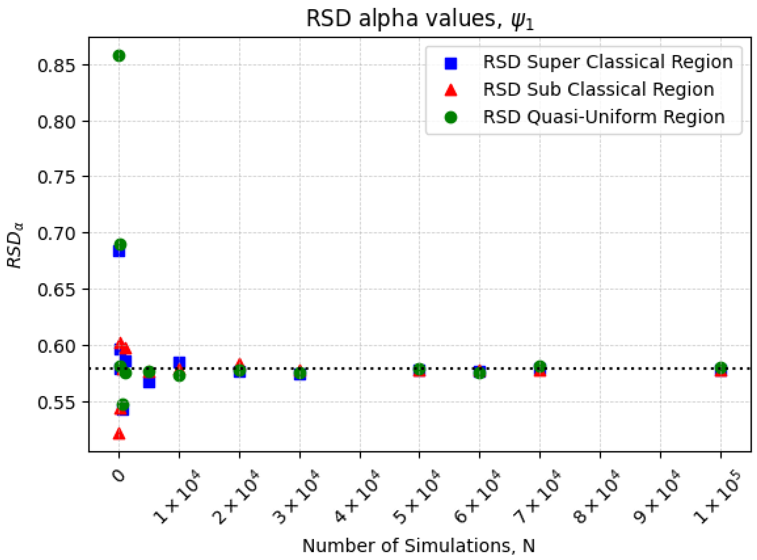
This methodology enables a rigorous and reproducible sensitivity analysis by employing Python-based Monte Carlo simulations to assess the impact of fractional-order derivatives on heat transfer behavior. Figure 2 and Figure 3 illustrate the relative standard deviation (RSD) of $\alpha$ as a function of the simulation size N for the conformable functions. The RSD is defined as:

$$RSD={\displaystyle \frac{s}{\overline{X}}}.$$

(18)

4. Results and Comparative Analysis of Thermal Regimes

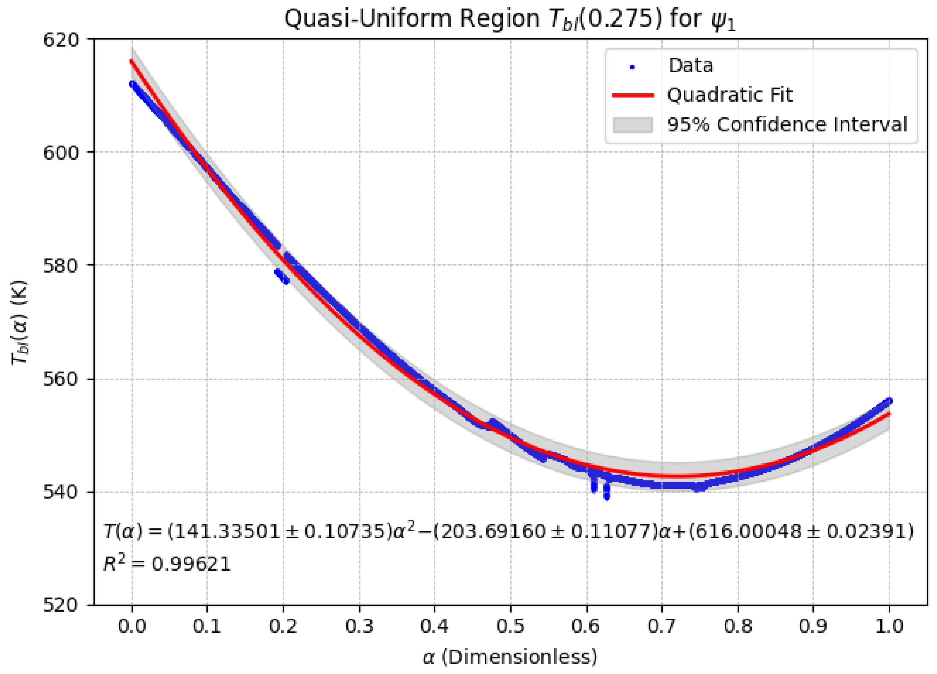
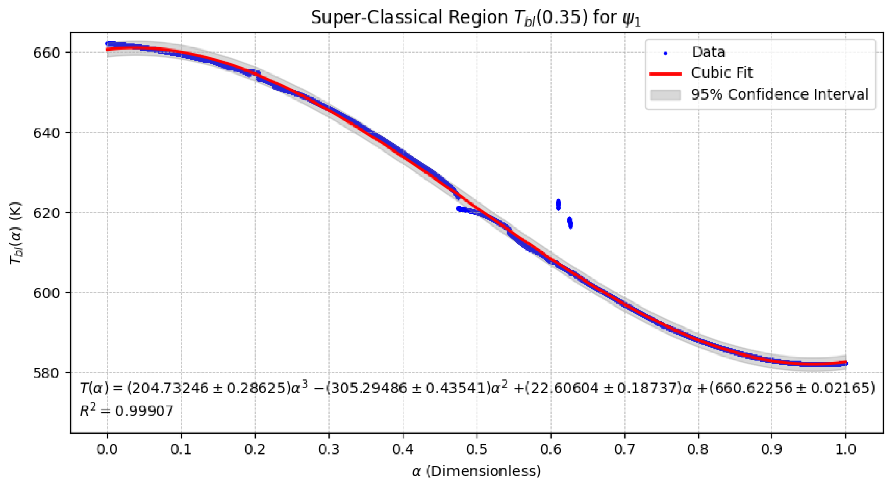
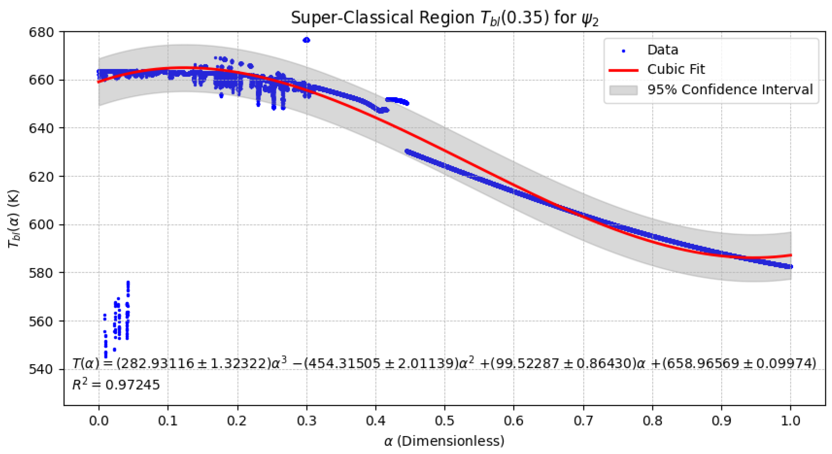
This section presents the results of the sensitivity and uncertainty analysis, followed by a detailed discussion of the observed trends. Figure 4 illustrates the behavior in the Quasi-Uniform Region using ${\psi }_1$, while Figure 5 presents the corresponding analysis with ${\psi }_2$. Figure 6 shows the results for the Super-Classical Region under ${\psi }_1$, where the cubic dependence reveals a consistent decrease in temperature as $\alpha$ increases. In contrast, Figure 7 displays the Super-Classical Region with ${\psi }_2$, maintaining the cubic behavior but showing broader confidence bounds, indicating greater variability in temperature response compared to ${\psi }_1$. 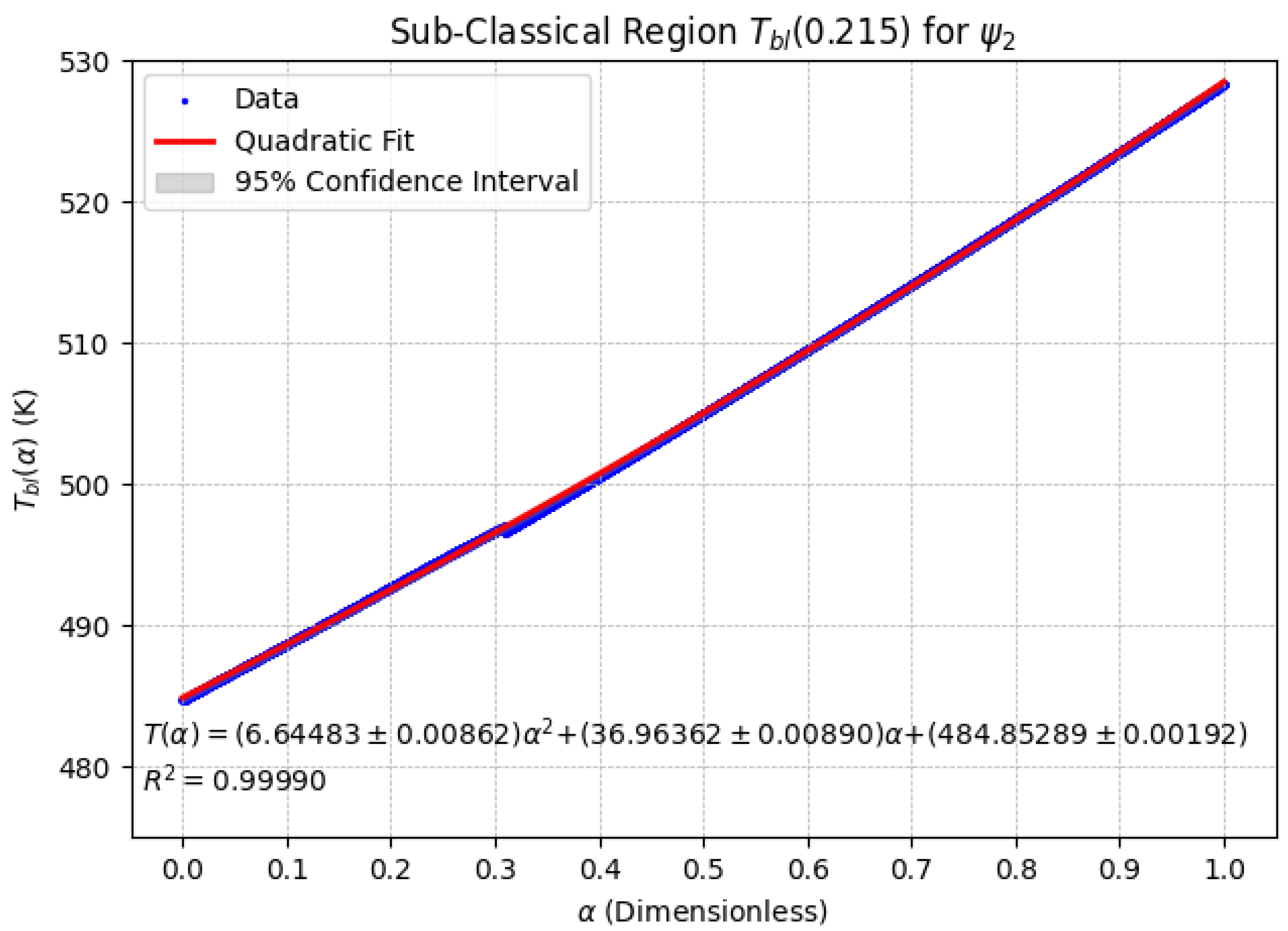Finally, Figure 8 presents the Sub-Classical Region using ${\psi }_1$, where a quadratic trend is observed with $T_{bl}\left(\alpha \right)$ increasing with $\alpha$, and Figure 9 shows a similar quadratic behavior for ${\psi }_2$, where $T_{bl}\left(\alpha \right)$ also increases as $\alpha$ grows.

Overall, both functions exhibit similar trends in their respective behaviors. However, a greater dispersion is observed in the data associated with ${\psi }_2$, indicating a higher sensitivity to parameter variations. This suggests that the choice of the conformable function significantly influences the thermal dynamics, which is crucial when modeling anomalous heat transfer mechanisms.

4.1. Analysis of the Quasi-Uniform Region

The thermal profile observed within the Quasi-Uniform Region is most accurately characterized by a quadratic regression model, which effectively captures the presence of a well-defined temperature minimum. As illustrated in Figure 4, the confidence interval (shaded in gray) associated with ${\psi }_1$ validates the robustness of this quadratic trend, indicating a high degree of precision in the estimation of thermal responses.

Figure 5 presents the corresponding analysis employing the function ${\psi }_2$. While the quadratic trend remains evident, the associated confidence interval is noticeably wider than that of ${\psi }_1$ (Figure 4), suggesting increased variability and reduced certainty in the thermal performance under this formulation.

The consistent emergence of quadratic temperature dynamics across both conformable functions suggests the presence of a stabilizing thermal mechanism within this regime. The temperature minimum identified in both cases may be interpreted as an optimal operational point, beyond which further increases in the fractional-order parameter $\alpha$ yield diminishing returns in thermal performance enhancement.

4.2. Analysis of the Super-Classical Region

In the Super-Classical Region, the temperature evolution exhibits a cubic relationship with respect to the fractional-order parameter $\alpha$. As shown in Figure 6, the blade temperature $T_{bl}\left(\alpha \right)$ under ${\psi }_1$ decreases monotonically with increasing values of $\alpha$, indicating a progressive enhancement in heat dissipation efficiency at higher fractional orders.

Figure 7 displays the corresponding behavior for ${\psi }_2$. While the cubic trend is similarly preserved, the thermal response exhibits increased fluctuations and is accompanied by a significantly broader confidence interval compared to that of ${\psi }_1$.

The persistence of cubic temperature dynamics across both conformable functions highlights the pronounced influence of the fractional-order parameter in this region. Notably, the more substantial modulation observed with ${\psi }_2$ underscores the sensitivity of thermal dynamics to the choice of conformable function, thereby emphasizing its critical role in designing effective thermal management strategies.

4.3. Comparative Analysis of the Second Super-Classical Region

The temperature evolution within the Sub-Classical Region exhibits a distinctly increasing trend, characterized by a third-degree (cubic) dynamic pattern, as illustrated in Figure 8. Interestingly, although the governing relationship is cubic, the response closely approximates a quadratic form in certain intervals. This behavior is observed when using the conformable function ${\psi }_1$.

The behavior of the Sub-Classical Region using ${\psi }_2$ is shown in Figure 9. It is highlighted that in this case, the confidence interval is thinner than shown in Figure 9 using ${\psi }_1$. The behavior was modeled using a cubic equation; however, it is remarkable that the dynamic represents quasi-linear behavior. That is, it exhibits a behavior that appears nearly linear, which could potentially obscure the underlying polynomial nature of the model.

In contrast to the previous region, here, $T_{bl}\left(\alpha \right)$ increases with $\alpha$, indicating that beyond a critical threshold, further increases in $\alpha$ lead to higher blade temperatures. This highlights the presence of a transition between different heat dissipation mechanisms, suggesting that $\alpha$ plays a pivotal role in determining thermal stability.

5. Optimal Selection of Fractional Order Parameters for Hydrogen Turbine Thermal Management

This section presents an optimization strategy designed to maximize blade temperature based on conformable derivative modeling. Given the asymptotic behavior described by Equation (15), it is established that, irrespective of the parameter $\alpha$ or the initial conditions, the long-term system dynamics converge to an attractor. Specifically, as time approaches infinity, the blade temperature stabilizes around $663.64$ K.

The focus of this analysis is to identify the values of $\alpha$ that maximize the temperature during the transient regime. To achieve this, a non-constant, time-dependent conformable parameter $\alpha \left(t\right)$ is considered, enabling the model to reach the highest theoretical temperatures at different time instances.

To establish this optimization framework, the study incorporates results obtained from the previously developed sensitivity analysis. These results provide regression-based approximations that link temperature to the parameter $\alpha$, thereby facilitating an analytical investigation of optimal thermal conditions.

Depending on the chosen conformable function $\psi$, the sensitivity regression yields either a quadratic or cubic expression in terms of $\alpha$. Let us consider two representative cases for modeling temperature $T_{bl}\left(\alpha \right)$.

First, suppose the temperature is approximated by a quadratic function of the form:

$$T_{bl}\left(\alpha \right)=A{\alpha }^2+B\alpha +C,\mathrm{with}\alpha \in ({\delta }_1,{\delta }_2).$$

(19)

In this case, the maximum value of $T_{bl}\left(\alpha \right)$ occurs at one of the endpoints $\alpha ={\delta }_1$ or $\alpha ={\delta }_2$, or at the critical point

$${\alpha }^{*}=-{\displaystyle \frac{B}{2A}},$$

(20)

provided ${\alpha }^{*}\in ({\delta }_1,{\delta }_2)$.

Alternatively, if the temperature is modeled by a cubic function as:

$$T_{bl}\left(\alpha \right)=A{\alpha }^3+B{\alpha }^2+C\alpha +D,\mathrm{with}\alpha \in ({\delta }_1,{\delta }_2),$$

(21)

the extrema of $T_{bl}\left(\alpha \right)$ are located at the endpoints or at the stationary points given by the solutions to the first derivative:

$${\alpha }^{*}={\displaystyle \frac{-B\pm \sqrt{B^2-3AC}}{3A}}.$$

(22)

Again, the feasibility of ${\alpha }^{*}$ as an optimal point depends on whether it lies within the admissible interval $({\delta }_1,{\delta }_2)$.

By applying this procedure to the sensitivity regression functions derived from both conformable functions ${\psi }_1$ and ${\psi }_2$, the corresponding values of $\alpha$ that maximize the transient temperature response are identified. This methodology enables the development of adaptive strategies wherein $\alpha$ is dynamically selected to enhance thermal performance throughout the system’s operational timeline.

Furthermore, based on the classification of the regions introduced earlier, the optimal values of the conformable order $\alpha$ that yield the maximum theoretical temperature for each case can be summarized.

In the Sub-Classical Region, the maximum theoretical temperature is attained when $\alpha =1$. In contrast, within the Quasi-Uniform Region, the optimal value corresponds to $\alpha =0$. Finally, for the Upper-Classical Region, the maximum temperature can be determined analytically by locating the critical points of the sensitivity regression functions.

For the conformable function ${\psi }_1$, the temperature is approximated by a cubic function, and the critical points are given by:

$${\alpha }^{*}={\displaystyle \frac{305.2949\pm \sqrt{{(-305.2949)}^2-3\left(204.7325\right)\left(22.6060\right)}}{3\left(204.7325\right)}}.$$

(23)

Solving this expression yields the stationary points ${\alpha }^{*}=0.9556$ (a local minimum) and ${\alpha }^{*}=0.0385$ (a local maximum).

Similarly, for the conformable function ${\psi }_2$, the critical points are:

$${\alpha }^{*}={\displaystyle \frac{454.3105\pm \sqrt{{(-454.3105)}^2-3\left(282.9312\right)\left(99.5229\right)}}{3\left(282.9312\right)}}.$$

(24)

This yields ${\alpha }^{*}=0.9466$ as a local minimum and ${\alpha }^{*}=0.1239$ as a local maximum.

Based on this behavior, a piecewise-defined function for the dynamic optimization of the conformable order $\alpha \left(t\right)$ is proposed, which switches depending on the temporal region of interest. For ${\psi }_1$, the optimal temporal dynamics of $\alpha$ can be modeled as:

$${\alpha }_1\left(t\right)=\left\{\begin{array}{cc}1\hfill & \mathrm{for}0\le t<0.275,\hfill \\ 0\hfill & \mathrm{for}t=0.275,\hfill \\ 0.0385\hfill & \mathrm{for}t>0.275.\hfill \end{array}\right.$$

(25)

Likewise, for ${\psi }_2$, the optimal temporal strategy is:

$${\alpha }_2\left(t\right)=\left\{\begin{array}{cc}1\hfill & \mathrm{for}0\le t<0.275,\hfill \\ 0\hfill & \mathrm{for}t=0.275,\hfill \\ 0.1239\hfill & \mathrm{for}t>0.275.\hfill \end{array}\right.$$

(26)

These dynamic models for $\alpha \left(t\right)$ provide an effective strategy to enhance thermal performance by maximizing the transient temperature response across distinct temporal regimes.

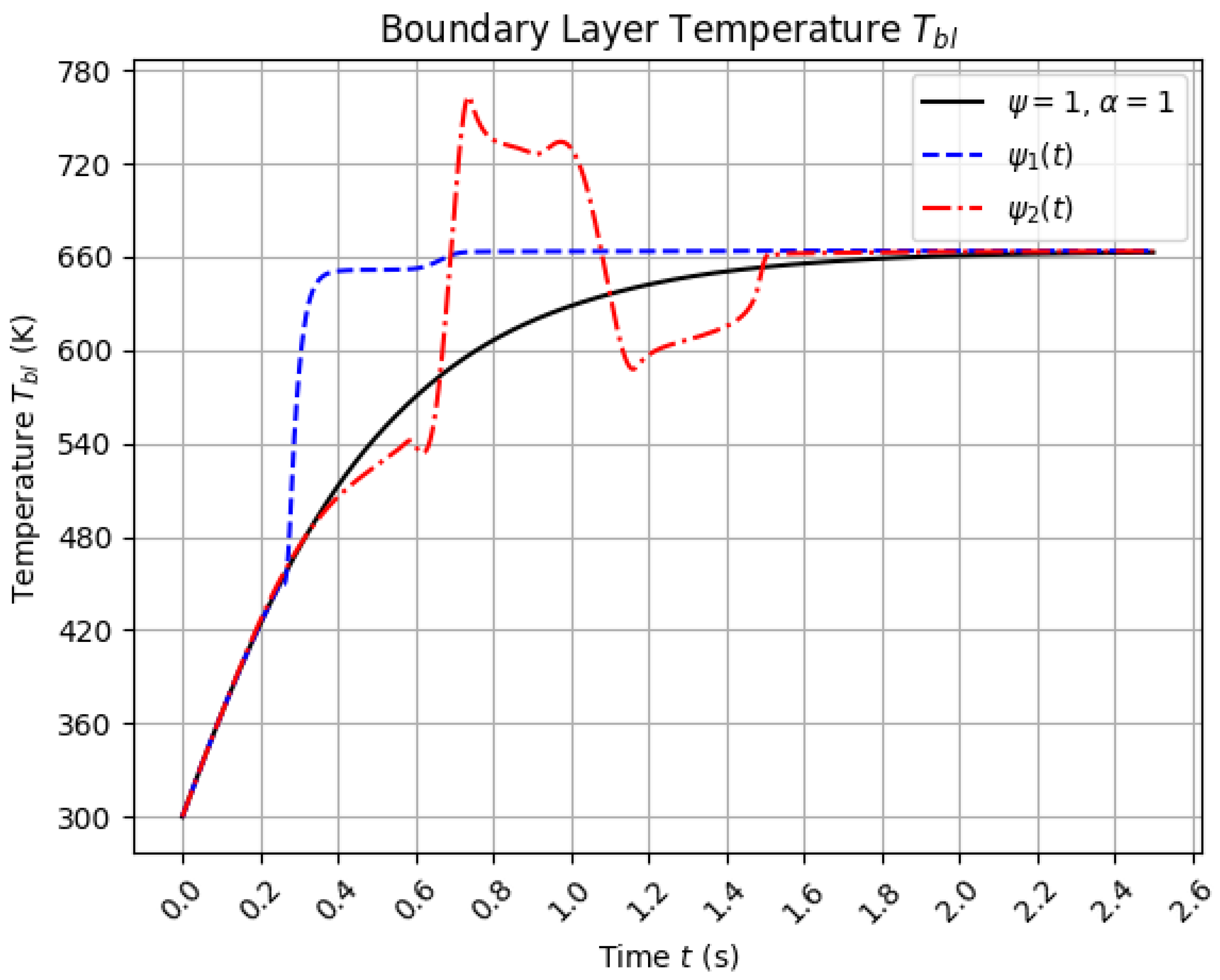
The optimal temperature behavior of the blade under different conformable dynamics is presented in Figure 10. It can be observed that employing the ${\psi }_2$ function allows the system to temporarily exceed the classical equilibrium temperature within the interval $(0.7,1.1)$ s. However, in the regions $(0.275,0.65)$ s and $(1.1,1.5)$ s, the temperature remains below that of the classical case. On the other hand, the use of ${\psi }_1$ leads to a significantly faster convergence toward equilibrium compared to the classical model, highlighting its potential for thermal performance enhancement in transient regimes.

The use of conformable functions such as ${\psi }_1$ and ${\psi }_2$ allows for distinct temperature profiles within the modeled system, each with specific practical implications. The function ${\psi }_2$ produces a transient overtemperature effect, where the system temporarily exceeds the classical equilibrium temperature. This behavior can be advantageous in processes that benefit from rapid heat input—such as ignition phases, rapid startups, or short-term thermal treatments—where improved heat transfer efficiency is desirable during the initial stage.

However, the transient overheating behavior induced by ${\psi }_2$ may introduce certain operational risks. Even short-duration temperature peaks can alter the thermal distribution within critical components, potentially increasing mechanical stress and accelerating failure mechanisms such as creep and low-cycle fatigue, particularly in high-temperature environments like gas turbines [24]. Moreover, the rapid thermal dynamics associated with ${\psi }_2$ may require advanced control strategies to ensure stability and safe operation, making its implementation more complex in practice.

In contrast, ${\psi }_1$ promotes a faster convergence toward thermal equilibrium without surpassing it. This results in a smoother, more stable temperature profile, which is beneficial in continuous industrial processes such as those found in turbines, heat exchangers, and thermal reactors. Such behavior minimizes thermal stress and improves long-term operational safety and efficiency. From an engineering perspective, the predictable and stable response of ${\psi }_1$ is often preferable in systems where safety, material longevity, and performance consistency are critical. These contrasting thermal responses also relate to fundamental thermodynamic insights, as described by Law (1989), who observed that entropy and velocity fluctuation coupling under strong temperature gradients can significantly alter system behavior [25].

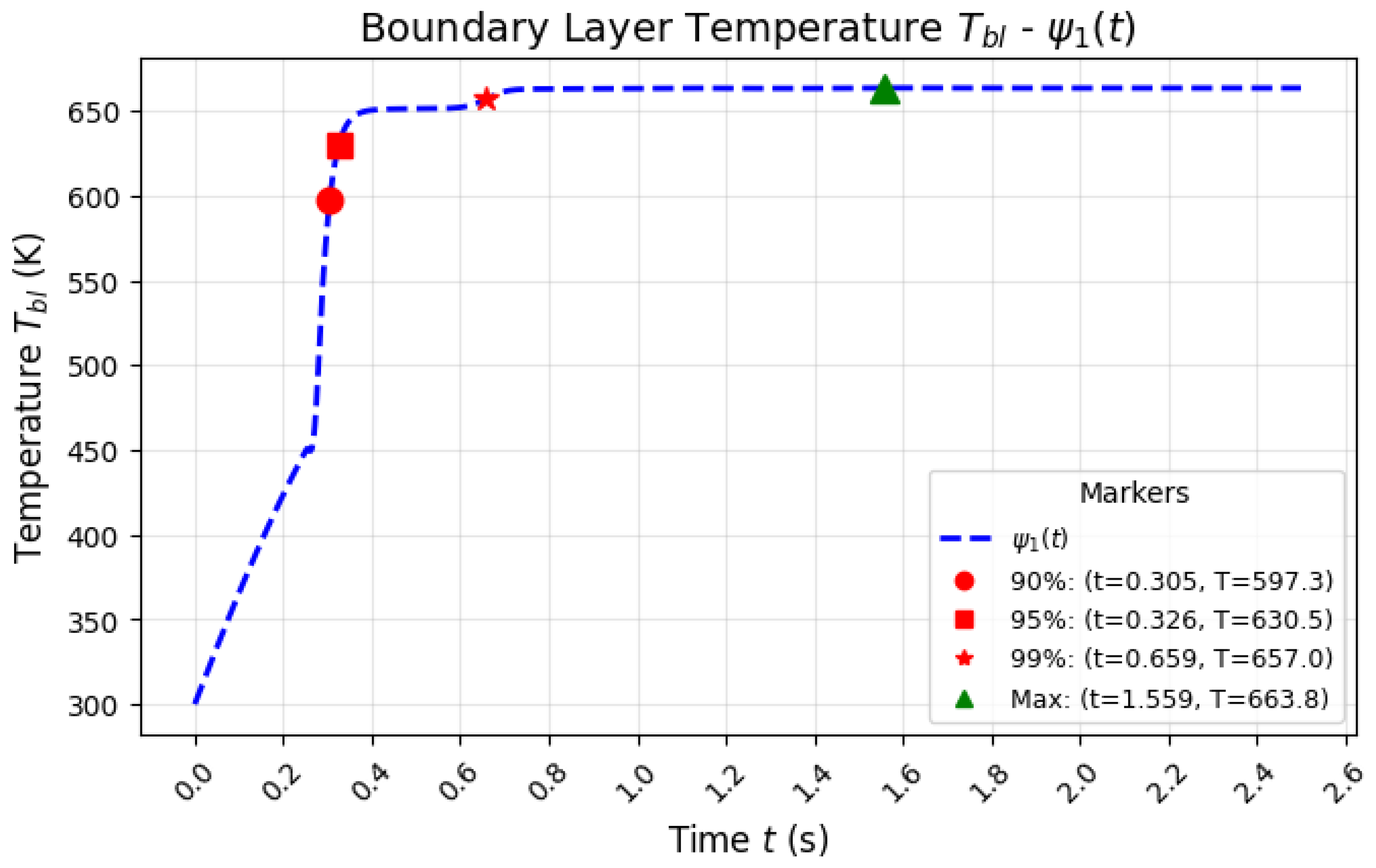
In the figures presented, the behavior of three models is analyzed in terms of their approach to equilibrium. Figure 11 illustrates the classical model, where the system gradually reaches 90%, 95%, and 99% of the equilibrium temperature over time. The time required for the system to reach these milestones is notably longer compared to the optimized models.

In contrast, Figure 12 shows the optimized model using ${\psi }_1\left(t\right)$, which accelerates the convergence towards equilibrium. The ${\psi }_1\left(t\right)$ model reaches the 90%, 95%, and 99% thresholds in significantly less time, demonstrating a more rapid and smoother approach to the final temperature. This behavior is further corroborated by the data presented in

Table 2. Times required to reach specific percentages of the maximum temperature, and the corresponding maximum temperature for each model.

Function	90% Time (s)	95% Time (s)	99% Time (s)	Max Temp (K)
Normal model	0.74 s	1.03 s	1.68 s	662.7 K
${\psi }_1\left(t\right)$	0.31 s	0.33 s	0.66 s	663.8 K
${\psi }_2\left(t\right)$	0.67 s	0.68 s	0.69 s	763.0 K

, where the times required for the model with ${\psi }_1\left(t\right)$ to reach each of these percentages are substantially shorter than those of the classical model.

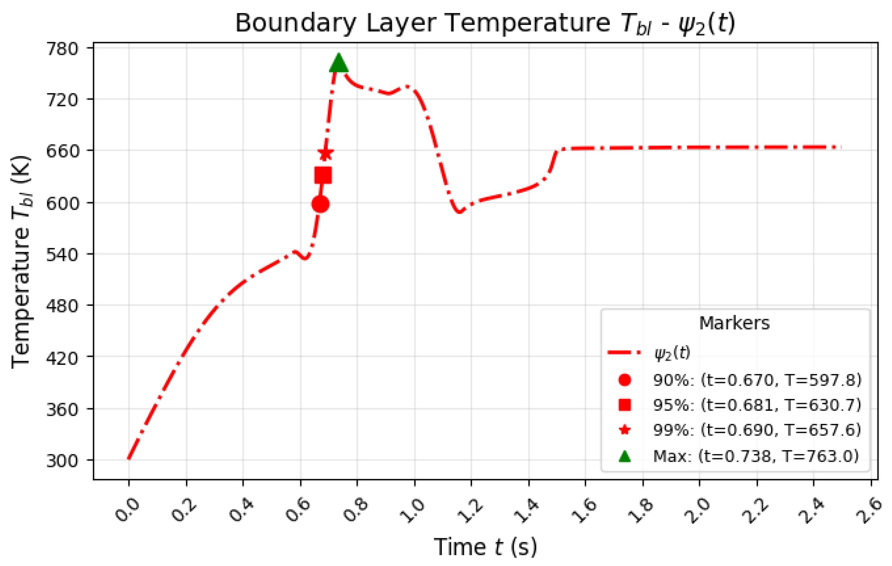
Figure 13 illustrates the behavior of the model optimized using ${\psi }_2\left(t\right)$, which also accelerates the convergence compared to the classical model. However, it is important to note that while the model with ${\psi }_2\left(t\right)$ reaches a higher maximum temperature (763.0 K), the approach to equilibrium is not as rapid or uniform as in the case of ${\psi }_1\left(t\right)$. The ${\psi }_2\left(t\right)$ model takes more time to reach the same percentages (90%, 95%, and 99%) of the equilibrium temperature, as shown in the table.

The comparison of these models in Table 2 clearly shows that the ${\psi }_1\left(t\right)$ model achieves the target temperatures in a shorter time, with a significantly quicker convergence to equilibrium. This makes the ${\psi }_1\left(t\right)$ model more advantageous in scenarios where speed is crucial, offering a more efficient system optimization process.

The higher peak temperature observed in the ${\psi }_2\left(t\right)$ model, while interesting, does not provide the same practical benefits in terms of system performance and efficiency. On the other hand, the rapid and smooth convergence of the ${\psi }_1\left(t\right)$ model is theoretically more beneficial for optimizing systems that require faster stabilization times.

In summary, the ${\psi }_1\left(t\right)$ model not only ensures faster convergence to equilibrium but also provides a more uniform and consistent thermal profile, making it a more effective choice for optimizing systems where both speed and stability are critical. The comparison of these results supports the theoretical advantages of using the ${\psi }_1\left(t\right)$ model in various applications, as illustrated in Figure 11, Figure 12 and Figure 13, along with the time data presented in Table 2.

6. Discussion and Implications

The results presented in

Table 3. Regression equations for the sensitivity of $T_{bl}\left(\alpha \right)$.

Case	Regression Equation	${\mathit{R}}^2$
Quasi-Uniform Region using ${\psi }_1$	$T_{bl}\left(\alpha \right)=(141.33501\pm 0.10735){\alpha }^2-(203.69160\pm 0.11077)\alpha +(616.00048\pm 0.2391)$	$0.99621$
Quasi-Uniform Region using ${\psi }_2$	$T_{bl}\left(\alpha \right)=(34.67172\pm 0.11824){\alpha }^2-(65.55953\pm 0.12217)\alpha +(586.97505\pm 0.02645)$	$0.96587$
Super-Classical Region using ${\psi }_1$	$T_{bl}\left(\alpha \right)=(204.73246\pm 0.28625){\alpha }^3-(305.29468\pm 0.43541){\alpha }^2+(22.60604\pm 0.18737)\alpha +(660.62256\pm 0.02165)$	$0.99907$
Super-Classical Region using ${\psi }_2$	$T_{bl}\left(\alpha \right)=(282.93116\pm 1.32322){\alpha }^3-(454.31505\pm 2.01139){\alpha }^2+(99.52287\pm 0.86430)\alpha +(658.96569\pm 0.09974)$	$0.97245$
Sub-Classical Region using ${\psi }_1$	$T_{bl}\left(\alpha \right)=(71.71414\pm 0.0429){\alpha }^2-(36.68746\pm 0.04432)\alpha +(419.26341\pm 0.00959)$	$0.99974$
Sub-Classical Region using ${\psi }_2$	$T_{bl}\left(\alpha \right)=(6.64483\pm 0.00682){\alpha }^2-(36.96362\pm 0.00890)\alpha +(484.85289\pm 0.00192)$	$0.9999$

highlight the distinct mathematical behavior of $T_{bl}\left(\alpha \right)$ in different regions, emphasizing the influence of the chosen conformable function. The Quasi-Uniform Region exhibits a quadratic trend with a well-defined minimum. Specifically, for ${\psi }_1$, the minimum occurs at approximately $\alpha =0.7206$, while for ${\psi }_2$, it is located at $\alpha =0.9454$. This suggests that the choice of conformable function influences not only the magnitude of $T_{bl}\left(\alpha \right)$ but also the critical points that define the system’s thermal performance.

In contrast, the Sub-Classical Region follows a nearly linear trend; however, a quadratic increasing function provided a better fit to the data. This indicates that in this regime, small variations in $\alpha$ lead to proportional changes in $T_{bl}\left(\alpha \right)$, reinforcing the idea that this region exhibits a more predictable and controlled thermal response.

The Super-Classical Region, on the other hand, is characterized by a cubic decreasing trend, where $T_{bl}\left(\alpha \right)$ diminishes as $\alpha$ increases. This behavior suggests that in this regime, higher values of $\alpha$ induce a stronger attenuation in temperature, which could have implications for thermal stabilization strategies in engineering applications.

One critical aspect to highlight is the overall quality of the regression fits. All Pearson correlation coefficients ($R^2$) exceed 0.97, ensuring that the proposed models accurately capture the underlying trends. It is also notable that when using ${\psi }_2$, the regression fits tend to exhibit slightly lower $R^2$ values and wider confidence intervals compared to those obtained with ${\psi }_1$. Additionally, to maintain statistical uniformity in the data, simulations with ${\psi }_2$ required 150,000 iterations, whereas ${\psi }_1$ achieved comparable results with only 100,000. This further reinforces the notion that ${\psi }_2$ is more sensitive to fractional-order changes than ${\psi }_1$.

The increased Monte Carlo sampling requirements for ${\psi }_2$ (150,000 samples versus 100,000 for ${\psi }_1$) highlight the need for further consideration of computational cost, particularly when extending the framework to multidimensional simulations. While the present study remains one-dimensional, scaling to higher dimensions would exponentially increase the sampling burden, thus reinforcing the importance of evaluating computational strategies. In this context, it is pertinent to situate the Monte Carlo method within its broader application in turbine research. For instance, Brusca et al. [26] employed a Monte Carlo-based characterization approach for a ducted Savonius turbine used in wave and wind energy recovery systems. Their methodology integrated experimental testing with high-fidelity CFD models, enabling the generation of performance curves through limited simulations, thus reducing the computational overhead. This highlights the versatility of Monte Carlo techniques not only for uncertainty quantification but also as a means to streamline the analysis of complex turbomachinery systems. Accordingly, the use of such methods in this study aligns with emerging trends in turbine modeling and optimization.

From a physical interpretation perspective, the variation of $T_{bl}\left(\alpha \right)$ with respect to $\alpha$ suggests that fractional-order derivatives could serve as a tuning parameter for temperature evolution. In the Quasi-Uniform Region, a minimum in $T_{bl}\left(\alpha \right)$ implies an optimal balance between heat accumulation and dissipation. In the Sub-Classical Region, the increasing trend of $T_{bl}\left(\alpha \right)$ indicates that as $\alpha$ grows, heat transfer mechanisms become more efficient in maintaining higher temperatures. Conversely, in the Super-Classical Region, the cubic decay of $T_{bl}\left(\alpha \right)$ with increasing $\alpha$ suggests that higher-order fractional effects contribute to enhanced thermal dissipation.

It is important to note that $\alpha$, as defined using the regression equations in (25) for ${\psi }_1$ and (26) for ${\psi }_2$, provides a flexible tool for tuning and optimizing the system’s thermal performance. The optimization of this parameter, guided by the regression models, can lead to improved control over the thermal dynamics in various operational environments.

These findings underscore the importance of carefully selecting the conformable function in fractional heat transfer models. The choice between ${\psi }_1$ and ${\psi }_2$ leads to distinct thermal behaviors, which must be considered when designing thermal management strategies. Future research should focus on the experimental validation of these theoretical predictions and their applicability in real-world engineering systems.

Optimization plays a crucial role in the context of the heat transfer dynamics discussed above, particularly in the fine-tuning of the parameters that govern the system’s response. The optimization of fractional-order derivatives in thermal models, such as the ones investigated in this study, provides a pathway to achieving more efficient and accurate thermal management solutions.

One key aspect to consider is the optimization of the choice of conformable function. Our results indicate that ${\psi }_1$ leads to more stable and efficient fits, with fewer iterations required for the model to converge. This suggests that ${\psi }_1$ may be optimized for practical applications where computational efficiency is critical. On the other hand, ${\psi }_2$ provided a better fit in terms of precision but at the cost of requiring more iterations, highlighting a trade-off between computational effort and accuracy. This difference emphasizes the importance of choosing an optimal function based on the specific needs of the thermal system being modeled.

Moreover, the regression analysis presented in Table 3 shows that the quality of the fit, as indicated by the $R^2$ values, is highly dependent on the selection of the conformable function and the corresponding fractional-order parameter. Optimization techniques, such as genetic algorithms or simulated annealing, could be employed to further refine these parameters, minimizing error and improving the predictive capability of the model.

In practice, this optimization can be extended to real-world applications, where fractional-order models may be used to optimize energy consumption, heat distribution, or thermal stabilization in complex systems. For example, in the design of thermal management systems, the ability to optimize $\alpha$ values and the conformable function can significantly enhance the system’s efficiency by improving heat transfer processes and minimizing energy losses. Additionally, optimization approaches that focus on minimizing the overall computational time while maintaining high accuracy will be essential for scaling these models to more complex, multidimensional systems.

Furthermore, the choice of optimization algorithm is also an important factor to consider. For instance, gradient-based methods may be effective when the objective function is smooth and differentiable, but for more complex, non-linear thermal systems with many local minima, global optimization techniques such as genetic algorithms or particle swarm optimization could provide better results. The application of these methods to the optimization of fractional-order thermal models would open new avenues for more advanced and adaptable thermal management strategies.

In conclusion, optimization not only aids in improving the accuracy of fractional heat transfer models but also ensures that these models are computationally feasible and practical for use in real-world engineering systems. Future research should explore various optimization techniques to further enhance the performance of these models and adapt them to dynamic, real-time thermal environments.

7. Conclusions

This study presents a comprehensive methodology heat management optimization for hydrogen turbine blades employing time-fractional conformable sensitivity analysis. Through the implementation of conformable derivatives and dynamic $\alpha \left(t\right)$ functions, complex heat transfer phenomena are captured, and optimal regimes for efficient thermal management are identified. The investigation yields significant theoretical insights and practical outcomes, advancing the field of fractional-order thermal modeling.

Three distinct thermal regions were identified—Quasi-Uniform, Sub-Classical, and Super-Classical—each exhibiting unique behaviors in response to variations in the fractional-order parameter $\alpha$. In the Quasi-Uniform Region ($t\in [0.26,0.29]$ s), the system demonstrated $\alpha$-invariant behavior, with temperature stabilizing at approximately 663.64 K. The Sub-Classical Region ($t\in [0.17,0.26]$ s) showed delayed thermal behavior for $\alpha \le 1$, with sensitivity analysis revealing a nearly linear or quadratic increasing trend. Conversely, the Super-Classical Region ($t\in [0.29,0.4]$ s) exhibited a cubic decreasing trend in $T_{bl}\left(\alpha \right)$, indicating enhanced heat dissipation as $\alpha$ increased.

Sensitivity analysis proved essential for quantifying the influence of $\alpha$ on the temperature dynamics and determining optimal values that maximize performance. The use of regression analysis (all $R^2>0.97$) confirmed the robustness of the identified trends. Notably, the function ${\psi }_2(t,\alpha )={(\xi sin\left(\theta t\right)+1)}^{1-\alpha }$ exhibited higher thermal sensitivity and required 150,000 Monte Carlo iterations to ensure statistical uniformity, compared to 100,000 for ${\psi }_1(t,\alpha )=e^{b(1-\alpha )sin\left(\theta t\right)}$. Although ${\psi }_2$ induced higher peak temperatures (763.0 K), ${\psi }_1$ showed superior stability and faster convergence.

To optimize the temperature $T\left(t\right)$, a piecewise definition of $\alpha \left(t\right)$ was constructed for both conformable functions, tailored to the thermal behavior in each region. This dynamic strategy led to a substantial reduction in time required to reach thermal equilibrium. Specifically, the time to reach 90%, 95%, and 99% of the equilibrium temperature was significantly decreased: by up to 60.7% for ${\psi }_1$ and 58.9% for ${\psi }_2$, relative to classical models. These results confirm the effectiveness of time-dependent fractional control in achieving faster thermal stabilization.

Importantly, the equilibrium behavior of the system remains unaffected by the conformable modeling. The final steady-state temperature is preserved across all values of $\alpha$, indicating that the conformable derivative primarily serves to capture transient, anomalous behaviors without altering long-term thermal balance. This validates the use of the conformable derivative as a robust tool to model non-classical dynamics while maintaining consistency with expected physical outcomes.

From an engineering perspective, the results offer valuable guidelines for turbine blade design. The ${\psi }_1$ function is particularly advantageous due to its rapid convergence with minimal fluctuations, making it ideal for applications requiring swift and stable thermal responses. Meanwhile, ${\psi }_2$ may be preferable in scenarios that benefit from transient overtemperature effects, such as rapid turbine startups. The optimal fractional-order values found—0.0385 for ${\psi }_1$ and 0.1239 for ${\psi }_2$—serve as key parameters for implementing real-time adaptive control.

Furthermore, the use of a piecewise definition for $\alpha \left(t\right)$ offers a flexible mechanism to simulate external perturbations or operational changes, thus extending the applicability of the model beyond stationary conditions. This enhances the model’s relevance for real-world applications where thermal inputs may vary over time.

Future Work and Research Outlook: Building upon the promising results of this study, several avenues for future research are proposed to further expand the applicability and depth of the conformable thermodynamic efficiency improvement framework. Although the current analysis was performed under idealized conditions with a one-dimensional heat transfer model and selected conformable functions, these assumptions serve as a foundational step toward more comprehensive modeling strategies.

To enhance the physical realism and predictive power of the proposed approach, future work will focus on:

• Experimental Validation: Implementation and testing of conformable heat transfer models under controlled laboratory conditions representative of turbine environments, enabling empirical calibration of fractional parameters and validation of model predictions.
• Geometric and Multidimensional Extensions: Integration of complex turbine blade geometries and multidimensional heat conduction effects into the conformable framework, allowing for spatially resolved temperature regulation optimization.
• Adaptive Control Algorithms: Development of real-time control algorithms for dynamically adjusting $\alpha \left(t\right)$ based on sensor feedback, thermal gradients, or external perturbations, enabling intelligent thermal regulation in evolving operating conditions.
• Coupled Thermo-Mechanical Modeling: Exploration of conformable derivatives in conjunction with mechanical fatigue, creep, and vibration models to provide a unified framework for structural-thermal co-design in high-performance turbine components.
• Generalization of Conformable Functions: Investigation of alternative and non-classical conformable functions beyond the canonical forms used in this work, to evaluate their sensitivity characteristics and modeling advantages in complex heat transfer scenarios.

These future developments will address the scope of the current formulation and significantly broaden its relevance and application in real-world engineering problems. The use of a piecewise-defined $\alpha \left(t\right)$ has already demonstrated its potential to simulate time-dependent external influences, such as fluctuating load conditions or environmental changes, providing a powerful and adaptable modeling tool.

Moreover, it is noteworthy that the equilibrium behavior of the system remains unaltered across all configurations of $\alpha$, reaffirming that the conformable approach does not distort the final steady-state outcomes. This property ensures that the methodology faithfully models anomalous and transient thermal phenomena without compromising the physical integrity of the system.

In summary, this work establishes a strong theoretical and computational foundation for the integration of conformable calculus into thermal performance enhancement. It opens a pathway for advanced adaptive modeling techniques in turbine design and energy systems, with considerable opportunities for refinement and practical implementation in future studies.