A Simple Analytical Approach to Estimating Solar Flux Distribution in a Multifaceted Solar Furnace Concentrator

Abstract

This study presents a theoretical analysis of the solar flux distribution within the receiver of the high-flux solar furnace at IER-UNAM. The furnace comprises an array of 409 first-surface spherical facets, each hexagonal in shape with a side length of 20 cm, and all mounted on a spherical framework. Each facet is carefully adjusted to focus sunlight onto a single focal point. Initially, the distribution of solar radiation is evaluated based on measurements obtained in Temixco, Morelos, Mexico (18°50′21″ N, 99°14′7.5″ W). Using these data, an analytical model is proposed to describe the solar radiation distribution using a Gaussian approximation. An additional analytical model is then developed to estimate the concentration distribution and its geometric shape at the furnace’s focal point, considering the solar width’s root mean square (RMS) value along with the optical errors associated with the heliostat and the reflective facets. Ultimately, by applying the concept of the effective solar source, an analysis of the solar flux distribution within the furnace receiver is conducted. This results in an analytical equation that characterizes the two-dimensional and three-dimensional distribution of the concentrated solar flux. Calculations reveal that the system captures approximately 30 kW of power, with peak concentrations reaching around 10,000 suns.

1. Introduction

Models of solar flux distribution within solar furnaces are critical for accurately predicting the sunlight concentration on the receiver’s surface. This is essential for optimizing energy capture efficiency and ensuring even heating across the surface, which is vital in preventing material failure. The primary methodologies used for this analysis include ray tracing techniques and various analytical models, each acknowledged for its specific advantages in enhancing the understanding and improvement of solar energy systems.

Ray tracing models can be categorized into two main types. Monte Carlo ray tracing simulates millions of solar rays reflecting off concentrator mirrors, effectively capturing complex optical phenomena such as multiple reflections, surface imperfections, and atmospheric effects. In contrast, deterministic ray tracing utilizes geometric optics to accurately calculate the paths of rays based on the system’s geometry. This method is beneficial for parametric studies, as it offers high accuracy in ideal conditions. The use of ray tracing methods has been thoroughly documented and explored in the academic community and literature.

Below are some representative articles discussing the concentrated solar flux distribution as the focus of a solar furnace:

In 2011, Lee et al. [1] developed a Monte Carlo ray tracing model incorporating solar limb darkening and reflector slope errors to simulate and analyze concentrated solar flux within a solar furnace. The model was rigorously validated against experimental data, demonstrating impressive concentration ratios highlighting its reliability and applicability in concentrated solar power research.

In 2013, the National Renewable Energy Laboratory (NREL) published a report detailing SolTrace [2], a versatile simulation utility intended to model the optical performance of concentrating solar power (CSP) systems. This tool effectively manages complex coordinate transformations and optical interactions, enabling precise predictions of solar flux distribution on receivers. Therefore, SolTrace is a valuable asset for optimizing the design and efficiency of CSP technologies.

In 2019, Cui et al. [3] conducted a study on the optical factors affecting the performance of solar furnaces. Their research utilized Monte Carlo ray tracing to investigate how optical errors, such as tilt and slope inaccuracies, influence solar flux distribution. The authors established acceptable ranges for these errors and provided design recommendations and guidelines.

In 2020, Pereira-Garcia et al. [4] conducted a comprehensive study comparing experimental measurements with ray tracing simulations in a high-flux SF60 solar furnace. The research explores critical factors such as beam alignment and the use of homogenizers, further examining the potential benefits of a double-paraboloid configuration to enhance flux uniformity. Their findings contribute significantly to our understanding of solar energy concentration methods and introduce advancements that could increase the efficiency of solar thermal energy applications.

Four years later, in 2024, Yi et al. [5] analyzed a 30 kWth reflective solar furnace designed for thermochemical reactions. Using the Monte Carlo ray tracing (MCRT) method, they validated their results against both SolTrace and experimental data. An improved four-quadrant focusing system was implemented to enhance flux distribution through inward crossover and platform movement. With direct normal irradiation (DNI) variations between 480 and 800 W/m², they achieved a non-uniformity factor of less than 0.10 and a peak flux ranging from 3000 to 3300 kW/m² while keeping fluctuations below 10%, thus ensuring stable thermochemical processes.

On the other hand, analytical models assume that the flux profile can be estimated using functions such as Gaussian distributions or cosine-powered functions. These approximations are easy to implement and function effectively for initial estimates in ideal, symmetric systems. Examples of this methodology include the following:

In 2018, Liu et al. [6] developed an analytical model to predict the solar flux distribution in parabolic trough solar furnaces using Gaussian approximations. This method simplifies complex flux profiles into Gaussian functions, enabling efficient intensity and spatial distribution estimations. Comparisons with numerical simulations demonstrate a strong agreement, thus validating the model for design optimization and performance evaluation in solar concentration systems. In 2019, Zhang and Li [7] introduced a Gaussian-based analytical model to describe the solar flux distribution in concentrating solar furnaces. This model effectively characterizes the flux profile through key parameters accounting for spatial variability and has been validated against experimental and simulated data. This method offers a reliable approach for predicting performance and supports the design and optimization of solar furnace systems.

In 2021, Wang et al. [8] conducted a study on the distribution of solar flux in an innovative solar furnace, employing both analytical modeling and experimental measurements. Their analytical model, which uses Gaussian approximations, strongly correlates with experimental results, confirming its accuracy. This research offers valuable insights into flux uniformity and concentration characteristics, contributing to design enhancements and operational control focused on improving thermal performance in solar furnaces.

In 2022, Kumar and Singh [9] developed an analytical model that uses Gaussian functions to predict solar flux distribution in a solar furnace. This model encompasses essential parameters that accurately simulate flux patterns, and its validity has been verified through comparisons with experimental data. Their approach enhances our understanding of flux variability and aids in developing more effective design and control strategies for solar furnace operations in cleaner production applications.

In 2023, Garcia et al. [10] conducted a comparative analysis of analytical and ray tracing models for solar flux distribution in high-flux solar furnaces. Their study evaluated the accuracy and efficiency of each method, revealing that analytical models—based on Gaussian assumptions—provide computational efficiency, while ray tracing models excel at offering enhanced spatial detail. These findings contribute to refining furnace designs and operational strategies to improve performance.

This study aims to present a clear analytical methodology for assessing the solar flux distribution within a complex solar furnace concentrator through geometric analysis. The straightforward analytical model characterizes the concentrated solar flux in the focal region of the High-Radiative Flux Solar Furnace (HRFSF) located in Temixco, Mexico, which operates at a power output of 30 kW with a concentration of 5000 suns. Designed to represent the solar flux distribution in both 2D and 3D, the model facilitates the generation of isocontours and gradient vector fields while allowing for analytical manipulation to examine the flux distribution across various planes. This comprehensive analysis clarifies the patterns of solar energy distribution within this high-performance system, enhancing the understanding of its operational effectiveness and potential applications in solar energy research.

The paper is structured to comprehensively analyze solar flux distribution in a high-flux solar furnace. Section 2 introduces the facility at IER-UNAM in Temixco, Mexico, detailing its design, operational parameters, and previous studies that support the current research. Section 3 explores the concept of sunshape, which refers to the radial energy distribution of incoming solar radiation. It elaborates on the theoretical foundation of sunshape and its crucial role in determining the performance of solar concentrators and the accuracy of solar flux predictions.

On the other hand, Section 4 describes the development and operation of the CCD Circumsolar Scope (CCS), an instrument designed to capture high-resolution sun images. This section outlines the instrument’s optical design—comprising lenses, filters, and a CCD sensor—and explains how the collected data are utilized to characterize the sun’s brightness profile. Furthermore, it introduces a novel continuous analytical model for solar intensity, employing Gaussian functions and incorporating the effects of optical errors through convolution to produce an effective source model. Section 5 details the geometric design and arrangement of the concentrator’s mirrors, including calculations for focal distances, mirror areas, and concentration ratios, illustrating how the physical layout impacts overall efficiency. Section 6 presents a two-dimensional analytical model that describes solar flux at the focal plane, while Section 7 extends the framework into three dimensions with corresponding volumetric equations, isosurfaces, and gradient fields.

Finally, Section 8 validates the models by comparing them with experimental data and ray tracing simulations. The concluding section summarizes the primary findings and their implications for enhancing solar furnace design and performance.

2. Background

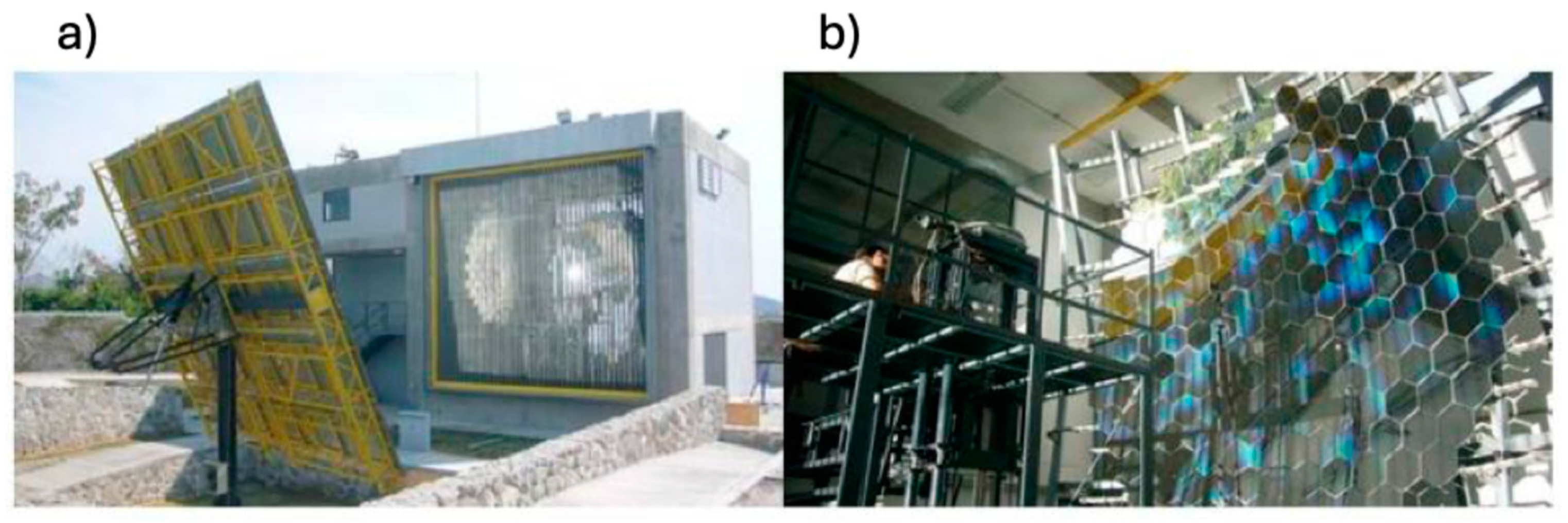
A high-flux solar furnace facility, known as the High Radiative Flux Solar Furnace (HRFSF) (see Figure 1), has been established at the Instituto de Energías Renovables in Temixco, Morelos, Mexico. This facility is designed to capture 30 kW of power, achieving a peak concentration of approximately 5000 suns and reaching temperatures as high as 3400 °C. To make the facility operational, all mirrors were carefully aligned, a control system was developed and tested, and the heliostat’s tracking mechanism was thoroughly verified [11,12,13]. This project received funding from Universidad Nacional Autónoma de México and Consejo Nacional de Ciencia y Tecnología.

During the design phase, various optical configurations were evaluated for the system’s concentrator. Ray tracing simulations were performed to analyze the distributions of concentrated radiative flux within the focal zone, facilitating comparisons among the different proposals. The optimal configuration was selected based on peak concentration, along with economic and practical considerations. The simulations referenced in [11] also examined the effects of optical errors.

In a previous study [12], an extensive 3D ray tracing analysis was conducted to investigate the behavior of the radiative distribution of concentrated solar radiation within the focal zone of a parabolic concentrator. A computer program was developed to generate isosurfaces of solar irradiance, ensuring a uniform radiation flux on the receiver surface. The program’s algorithm introduces a methodology for deriving flux isosurfaces across various optical configurations. The study evaluated the impact of optical errors on the mirror surface and examined different mirror shapes, including round, square, and faceted designs. Numerical calculations were performed using the convolution ray tracing technique. However, the methodology employed in this research was somewhat cumbersome, requiring a significant number of ray-tracing simulations to construct the isosurfaces. In another study, researchers conducted a theoretical analysis to explore the effects of facet size and optical errors on multiple-facet point-focus of solar concentrating systems. The results indicated that both the facets’ size and their optical inaccuracies significantly influence the system’s peak concentration and optimal focal distance [13].

In the following section, the distribution of energy is examined in relation to the radial distribution of incoming solar energy, referred to as the sunshape. A measurement system known as the CCD Circumsolar Scope (CCS) was designed to capture an accurate solar image and analyze this sunshape. Additionally, a model was created to represent the brightness of the solar disk and elaborate on the aureole.

3. Sunshape Distribution

In solar concentration systems, energy distribution is significantly influenced by the radial distribution of incoming solar energy, a phenomenon commonly referred to as the sunshape. Numerous studies have focused on developing a representative angular brightness profile to enhance the calculation of this irradiance [14,15,16,17,18]. To effectively characterize the sunshape, researchers have developed models that integrate two distinct functions: one representing the brightness of the solar disk and another depicting the aureole. These functions are affected by solar limb darkening and small-angle scattering in the atmosphere, caused by phenomena such as Mie and Rayleigh scattering [15].

When the particle size is significant relative to the wavelength—typically ranging from 0.1 µm to 1 µm [16]—small-angle forward scattering occurs, leading to the formation of the solar aureole as observed from the Earth’s atmosphere [17]. The energy contained in this region, known as the circumsolar region or solar aureole, is vital for solar concentration systems. This importance arises from the fact that, depending on the system’s acceptance angle, the concentrated solar flux may be overestimated if it is assumed that all power resides solely within the image of the solar disk [18]. Furthermore, the radial energy profile (sunshape) plays a crucial role in influencing the distribution of the concentrated solar flux within the focal plane.

4. Sunshape Measurement System

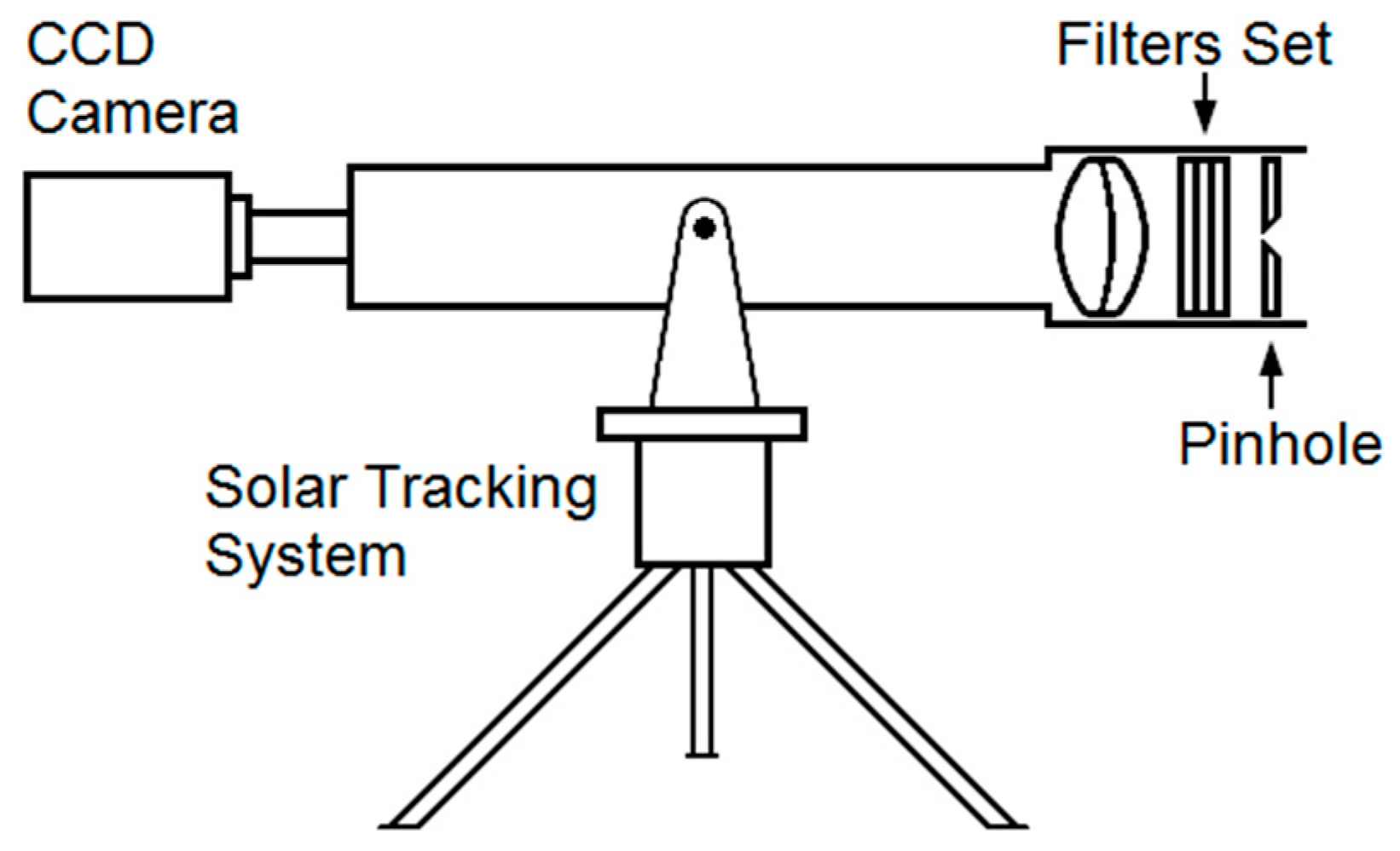
A solar shape measurement system, known as the CCD Circumsolar Scope (CCS), was developed at the Institute of Renewable Energies, National Autonomous University of Mexico (IER-UNAM). This advanced instrument is specifically designed to capture direct images of the sun. The CCS includes an achromatic lens with a focal length of 670 mm, which is directly coupled to an Allied Pike camera that uses a 16-bit CCD sensor with dimensions of 16 × 9 mm². To modulate solar light intensity, a 5 mm diameter pinhole, along with a series of neutral density filters, is employed, achieving a total optical density of 6. This specific optical density has been carefully chosen to ensure that the dynamic intensity range remains well below the saturation threshold of the CCD sensor. The complete system is mounted on a solar tracking apparatus, and the overall configuration is illustrated in Figure 2.

The CCS was employed in a measurement campaign from March 2023 to September 2024, capturing images of the sun on clear days. The high-quality images obtained will aid in creating a database that will help establish solar distribution patterns across different seasons.

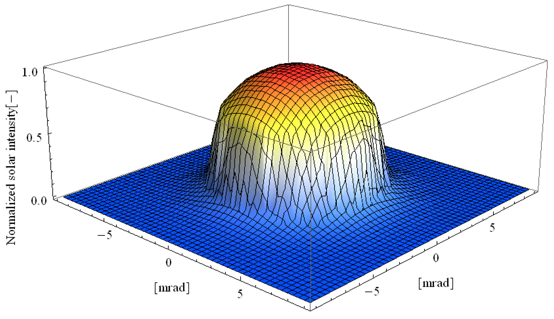
Figure 3 shows an image of the sun taken under a very clear sky. The grayscale distribution was processed using Image Processing & Analysis from the Mathematica Software^TM. The same figure displays the profile of the solar distribution. It is important to note that this distribution is used to model the behavior of the HRFSF.

4.1. A Novel Sunshape Analytical Model

This section introduces a novel mathematical model of the sunshape. This model provides a continuous mathematical expression that is both derivable and integrable with respect to angular displacement, allowing for comprehensive analysis and application in relevant disciplines. In the context of solar energy assessment, if it is posited that the solar intensity profile illustrated in Figure 3 exhibits radial symmetry—a hypothesis that aligns well with established understanding of solar distributions [19]—and the radiant flux corresponding to the solar image can be articulated as follows:

$$I_s={\int }_0^{2\pi }{\int }_0^{{\beta }_{\Delta }}B\left(\beta \right)\hspace{0.17em}\sin \left(\beta \right)\hspace{0.17em}d\beta d\psi$$

(1)

since β is a small quantity, it is possible to write

$$I_s=2\pi {\int }_0^{{\beta }_{\Delta }}B\left(\beta \right)\hspace{0.17em}d\beta$$

(2)

where I_s is the normalized solar irradiance, β is the radial angular displacement and β_Δ = 10.75 mrad is the radial angular size of the solar disk plus circumsolar region. In this work, the value of β_Δ is defined by the aperture of the CCS. In the literature, the circumsolar region is considered to extend further than 10.75 mrad [15,16]. However, for the purpose of analyzing the distribution of concentrated solar flux, the range measured in this work is deemed sufficient.

A novel continuous function that describes the energy distribution from 0 to β_Δ is proposed to model the solar intensity profile,

$$B\left(\beta \right)=a+\left(b-a\right)\hspace{0.17em}\left({\displaystyle \frac{c}{1+{10}^{-d\left(e-\beta \right)}}}+{\displaystyle \frac{1-c}{1+{10}^{-f\left(g-\beta \right)}}}\right)$$

(3)

where the constants are a = 0.03363, b = 0.98966, c = 0.53307, d = −0.50323, e = 3.83744, f = −6.46188, g = 4.59596, which are the values of the fitting parameters employed for the data in Figure 2.

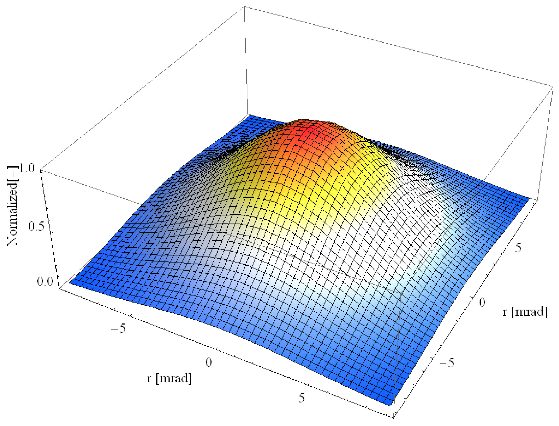
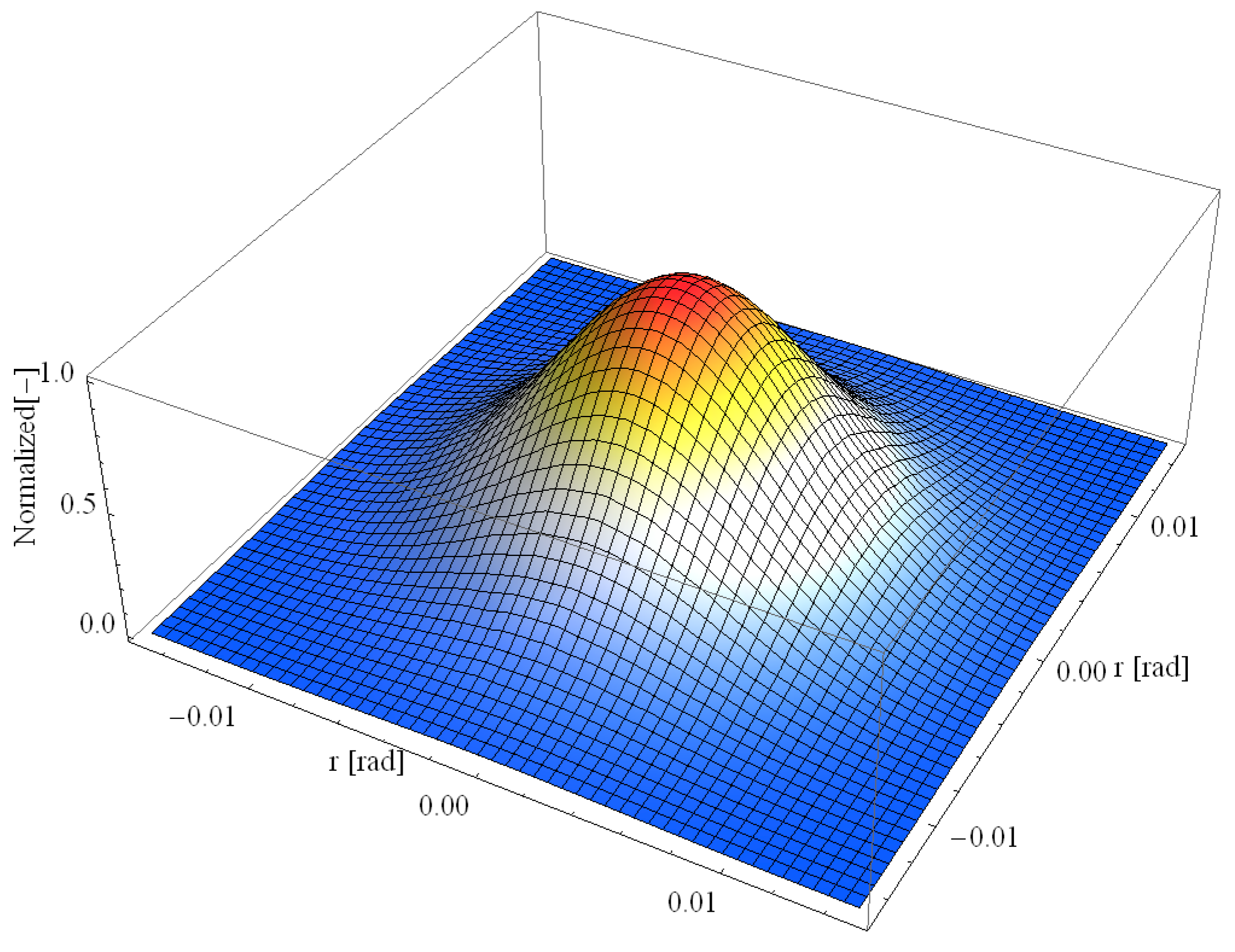
In the context of assuming rotational symmetry in the intensity distribution B(β), a two-dimensional brightness map illustrating both the solar and circumsolar brightness can be effectively represented, as shown in Figure 4. This approach allows for a comprehensive visualization of brightness variations across the specified regions.

The boundary of the solar disk undergoes minor variations throughout the year due to fluctuations in the Earth–sun distance; however, a standard value of 4.65 mrad is generally accepted. In contrast, actual solar brightness distributions can vary significantly based on atmospheric conditions. Under hazy skies, the radiation emanating from the solar disk decreases, while circumsolar radiation increases noticeably compared to conditions characterized by clarity.

For the statistical analysis of the radiation intercepted by a solar concentrator, it is suitable to use the rms width of the sun rather than its radius. For point-focus geometry, the rms width σ_s is given by [19]

$${\sigma }_s^2={\displaystyle \frac{{\int }_0^{\infty }B\left(\beta \right)\hspace{0.17em}{\beta }^{3}d\beta }{{\int }_0^{\infty }B\left(\beta \right)\hspace{0.17em}\beta d\beta }}$$

(4)

It is important to indicate that, for real solar brightness distribution, the rms width varies with the atmospheric conditions. Under a very clear sky and an average clear sky, the width is [19]

$${\sigma }_s\approx 3.6\hspace{0.17em}\mathrm{mrad} \left(5.6\hspace{0.17em}\mathrm{mrad}\right)\hspace{0.17em} \mathrm{Very} \mathrm{Clear} \mathrm{Sky}, (\mathrm{Average} \mathrm{Clear} \mathrm{Sky})$$

(5)

From the previous model of B(β) (Equation (3)), σ_s = 4.47 mrad is obtained:

$${\sigma }_s=\sqrt{\left({\displaystyle \frac{{\int }_0^{{\beta }_{\Delta }}\left(a+\left(b-a\right)\hspace{0.17em}\left(\frac{c}{1+{10}^{-d\left(e-\beta \right)}}+\frac{1-c}{1+{10}^{-f\left(g-\beta \right)}}\right)\right)\hspace{0.17em}{\beta }^{3}d\beta }{{\int }_0^{{\beta }_{\Delta }}\left(a+\left(b-a\right)\hspace{0.17em}\left(\frac{c}{1+{10}^{-d\left(e-\beta \right)}}+\frac{1-c}{1+{10}^{-f\left(g-\beta \right)}}\right)\right)\hspace{0.17em}\beta d\beta }}\right)}$$

(6)

this value, σ_s = 4.47 mrad, shows a very good condition in the atmosphere of Temixco, Mexico, for the particular day under analysis.

Once the measurement yields σ_s = 4.47 mrad, it becomes advantageous for the calculation of the solar concentrator system to approximate the solar irradiance distribution using a Gaussian function, denoted as B_s(β). This approach allows for a simplified analytical treatment of the solar input characteristics. The Gaussian representation can be mathematically expressed as follows:

$$B_s\left(\beta \right)=\exp \left(-{\displaystyle \frac{1}{2}}\left({\left({\displaystyle \frac{\beta }{{\sigma }_s}}\right)}^2\right)\right)$$

(7)

Representing the sun’s shape with a Gaussian distribution is a practical and effective approach. This method simplifies the intricate angular intensity profile of sunlight by approximating it with a symmetric bell curve, thereby making calculations more straightforward. It is commonly employed in simulations of solar concentrators and solar furnaces, allowing researchers to estimate the distribution of solar radiation across the solar disk. The Gaussian model strikes a balance between simplicity and a realistic portrayal of solar flux patterns [14]. The approximation of the solar brightness distribution by a Gaussian distribution with σ_s = 4.47 mrad is depicted in Figure 5.

It is important to notice that integral in 2D of Gaussian B_s(β) from 0 to β_Δ amounts only to the 95% of the energy contained in the real solar brightness distribution in Equation (3), as shown by Equation (8). However, the calculations of the concentrated solar flux intercepted in the focal plane are not affected by this model since the useful information within the Gaussian representation is in the central part and not on the outskirts.

$$E_{Bs}={\displaystyle \frac{1}{\left(2\pi \right)\hspace{0.17em}\left({\sigma }_s^2\right)}}{\int }_0^{2\pi }{\int }_0^{{\beta }_{\Delta }}\exp \left(-{\displaystyle \frac{1}{2}}\left({\left({\displaystyle \frac{\beta }{{\sigma }_s}}\right)}^2\right)\right)\hspace{0.17em}\beta d\beta d\psi \cong 0.95$$

(8)

4.2. Effective Source for the Solar Furnace

The effective source for the solar furnace can be estimated by considering the convolution of the B_s(β) and the optical errors associated with the mirrors facets, the heliostat, and the tracking system. The resulting effective source is also a Gaussian distribution:

$$B_{eff}\left(\beta \right)={\displaystyle \frac{1}{\left(2\pi \right)\hspace{0.17em}\left({\sigma }_T^2\right)}}\exp \left(-{\displaystyle \frac{1}{2}}\left({\left({\displaystyle \frac{\beta }{{\sigma }_T}}\right)}^2\right)\right)$$

(9)

where σ_T is given by

$${\sigma }_T^2={\sigma }_s^2+{\sigma }_{optical}^2$$

(10)

and σ_optical is the standard deviation that accounts for all optical errors. The latter is given by the quadratic sum of the individual errors, namely,

$${\sigma }_{optical}^2={\sigma }_{Facets}^2+{\sigma }_{Heliostat}^2+{\sigma }_{Tracking}^2$$

(11)

Dynamic solar tracking systems with adjustable facet angles can be incorporated into the model by adding two additional terms to Equation (11): σ_displacement, which represents the orientation of the heliostat towards the sun, and σ_contour, which defines the variation in the facet angle.

In the present case, these errors have the values σ_Facets = 1.0 mrad, σ_Heliostat = 2.0 mrad, and σ_Tracking = 2.0 mrad. These values have been estimated from previous designs of the HRFSF (12). Therefore, the value of σ_T is

$${\sigma }_T=5.38\hspace{0.17em}\mathit{mrad}$$

(12)

The integral in 2D of the symmetrical Gaussian distribution B_eff(β) for 2σ_T (that is, from −2σ_T to 2σ_T), amounts to 95% of the energy contained in the solar brightness distribution, i.e.,

$$B_{Beff}\left(\beta \right)={\displaystyle \frac{1}{\left(2\pi \right)\hspace{0.17em}\left({\sigma }_T^2\right)}}\exp \left(-{\displaystyle \frac{1}{2}}\left({\left({\displaystyle \frac{{\beta }_x}{{\sigma }_T}}\right)}^2+{\left({\displaystyle \frac{{\beta }_y}{{\sigma }_T}}\right)}^2\right)\right)\hspace{0.17em}$$

(13)

$$E_{Beff}={\displaystyle \frac{1}{\left(2\pi \right)\hspace{0.17em}\left({\sigma }_T^2\right)}}{\int }_{-2{\sigma }_T}^{2{\sigma }_T}{\int }_{-2{\sigma }_T}^{2{\sigma }_T}\exp \left(-{\displaystyle \frac{1}{2}}\left({\left({\displaystyle \frac{{\beta }_x}{{\sigma }_T}}\right)}^2+{\left({\displaystyle \frac{{\beta }_y}{{\sigma }_T}}\right)}^2\right)\right)\hspace{0.17em}d{\beta }_{x}d{\beta }_y$$

(14)

Considering the above, the resulting effective source of the HRFSF can be modeled as a circular Gaussian shape which subtends an angle of

$$\begin{array}{l}{B}_s=4{\sigma }_T\\ B_s=21.54\hspace{0.17em}\mathrm{mrad}\end{array}$$

(15)

In other words, a Gaussian solar ray bundle, reflected from any of the mirrors of the concentrator to the focal point of the array, from −2σ_T to 2σ_T, spans 95% of the power contained in the solar brightness distribution. Figure 6 depicts the effective Gaussian brightness distribution.

5. Geometrical Concentration of the Multifaceted-Concentrator Solar Furnace

Using a method similar to that outlined in reference [10], the concentration ratio for the HRFSF is determined through a geometric optics-based model. The HRFSF is composed of 409 hexagonal first-surface polished glass mirrors featuring an aluminum coating. These mirrors are mounted on a frame that exhibits a spherical curvature with a radius of 7.36 m, as depicted in Figure 7. The overall structure is measured at approximately 3.25 m in height and 3.5 m in width. The origin of the coordinate system is established at the vertex of the central mirror, allowing for the precise identification of the position (x, y, z) of each mirror’s vertex. The focal distances of the mirror facets are grouped into five categories, each corresponding to a specific focal distance, as outlined in

Table 1. Focal distances of mirrors from different groups.

Group	f [cm]
A	375.0
B	400.0
C	425.0
D	450.0
E	475.0

. The area A_m of each hexagonal mirror is computed as:

$$\begin{array}{cc}\hfill L& =20\hspace{0.17em}\mathrm{cm}\hfill \\ \hfill Apothem& =\sqrt{L^2-{\left({\displaystyle \frac{L}{2}}\right)}^2}\hfill \\ \hfill Perimeter& =L\times 6\hfill \\ \hfill A_m& ={\displaystyle \frac{Apothem\times Perimeter}{2}}\hfill \\ \hfill A_m& =1039.23\hspace{0.17em}{\mathrm{cm}}^2\hfill \end{array}$$

(16)

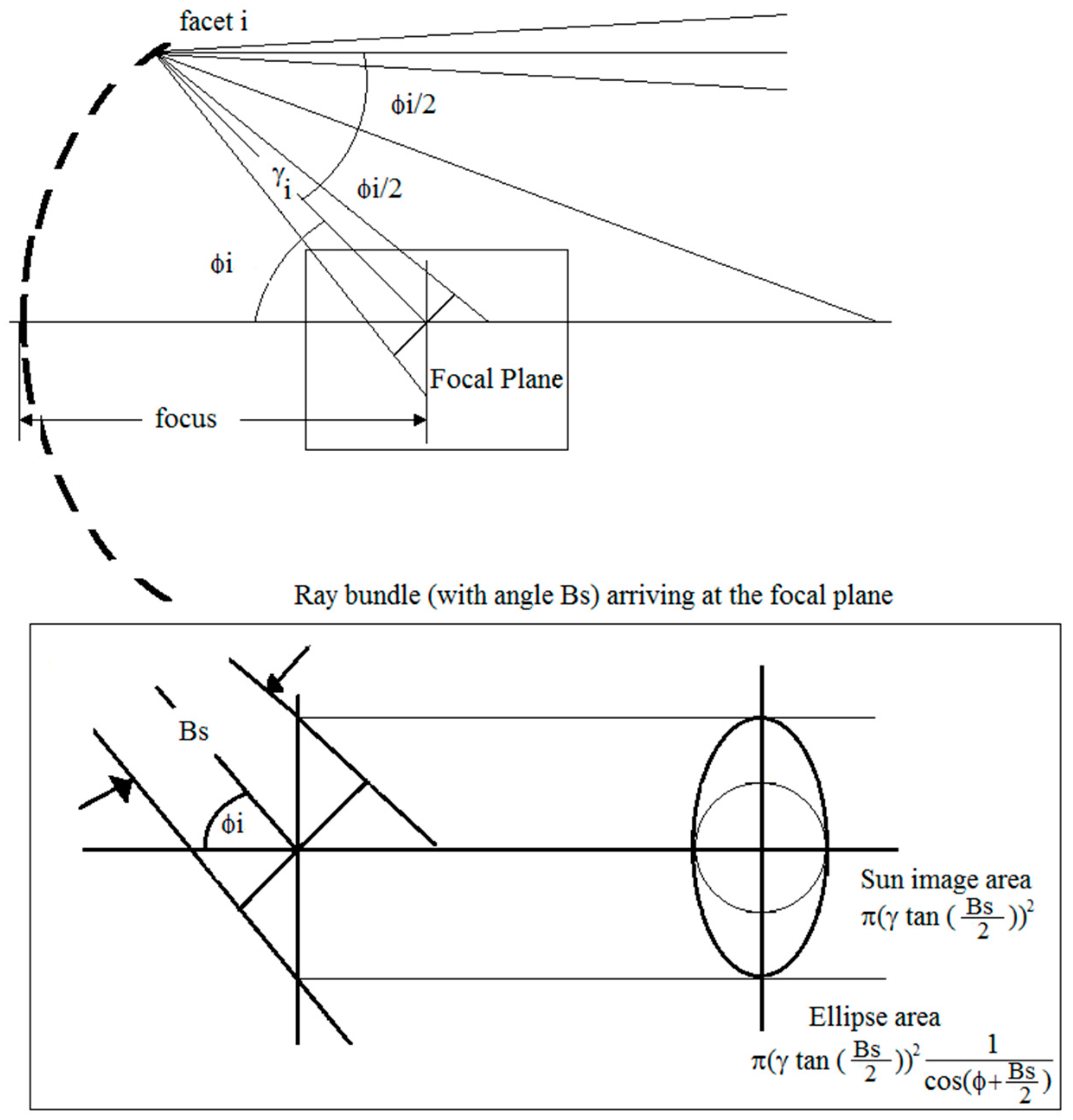
On the other hand, a solar ray bundle reflected from a concentrator mirror i to the focal point of the array (located at (0, 0, 368)cm) produces a circular image with an area:

$$S_i=\pi {\left({\gamma }_i\tan \left({\displaystyle \frac{Bs}{2}}\right)\right)}^2$$

(17)

where γ_i is the distance between the focal point of the array and the vertex of the mirror i. This distance can be calculated by solving

$${\gamma }_i=\sqrt{x_i^2+y_i^2+{\left(focus-z_i\right)}^2}$$

(18)

and focus = 368 cm is the distance from the focal point of the array to the center of the array as shown in Figure 8.

In a plane normal to the optical axis, the solar image from each mirror becomes an ellipse of diminished intensity, whose area can be estimated by

$$E_{A,\hspace{0.17em}i}=S_i{\displaystyle \frac{1}{\cos \left({\phi }_i+\frac{Bs}{2}\right)}}$$

(19)

where ϕ_i is the angle between the optical axis and the normal vector at the vertex of the mirror i, namely,

$${\phi }_i=\arccos \left({\displaystyle \frac{focus-z_i}{{\gamma }_i}}\right)$$

(20)

The concentration ratio attributable to a particular mirror i is given by

$$c_i={\displaystyle \frac{A_{eff,\hspace{0.17em}i}}{E_{A,\hspace{0.17em}i}}}={\displaystyle \frac{A_m\cos \left(\frac{{\phi }_i}{2}\right)}{E_{A,\hspace{0.17em}i}}}$$

(21)

where A_eff,i is the projected area of the mirror in a plane normal to the optical axis, and E_A,i is the area of the ellipse in the focal plane normal to the axis. Therefore, the concentration ratio for the solar furnace is determined by

$$C_T={\displaystyle \sum }_{i=1}^{409}{\displaystyle \frac{A_{eff,\hspace{0.17em}i}}{E_{A,\hspace{0.17em}i}}}=5148.9$$

(22)

In

Table 2. Contribution of each mirror to the concentration ratio.

Group	N	f [cm]	Γ [cm]	ϕ [°]	Aeff,i [cm2]	N Aeff,i [cm2]	Sun Image Area [cm2]	Ellipse Area [cm2]	Ci [-]	N Ci [-]
A	1	375.0	368.00	0.0	1039.2	1039.2	49.3	49.3	21.1	21.1
A	6	375.0	368.86	5.5	1038.0	6228.1	49.6	49.9	20.8	124.8
A	6	375.0	370.56	9.5	1035.6	6213.8	50.0	50.9	20.3	122.0
A	6	375.0	371.41	11.0	1034.4	6206.7	50.2	51.4	20.1	120.7
A	12	375.0	373.94	14.5	1030.9	12,371.0	50.9	52.9	19.5	233.8
A	6	375.0	375.61	16.4	1028.6	6171.6	51.4	53.9	19.1	114.4
A	6	375.0	378.11	18.9	1025.2	6150.9	52.1	55.5	18.5	110.9
A	12	375.0	378.93	19.6	1024.0	12,288.2	52.3	56.0	18.3	219.5
A	6	375.0	381.40	21.7	1020.6	6123.9	53.0	57.5	17.7	106.4
A	12	375.0	383.85	23.6	1017.3	12,207.8	53.7	59.1	17.2	206.5
A	12	375.0	385.47	24.7	1015.1	12,181.5	54.1	60.2	16.9	202.4
B	6	400.0	388.68	26.9	1010.8	6064.8	55.0	62.4	16.2	97.2
B	6	400.0	390.27	27.9	1008.7	6052.1	55.5	63.5	15.9	95.3
B	12	400.0	391.07	28.3	1007.6	12,091.4	55.7	64.0	15.7	188.8
B	12	400.0	393.44	29.7	1004.5	12,053.7	56.4	65.7	15.3	183.3
B	6	400.0	397.35	31.9	999.3	5995.9	57.5	68.6	14.6	87.3
B	12	400.0	398.12	32.3	998.3	11,979.6	57.7	69.2	14.4	173.0
B	12	400.0	399.67	33.1	996.3	11,955.4	58.2	70.4	14.1	169.8
B	12	400.0	402.74	34.6	992.3	11,907.5	59.1	72.8	13.6	163.5
B	24	400.0	407.10	36.6	986.7	23,680.2	60.4	76.4	12.9	309.8
B	12	400.0	409.53	37.7	983.6	11,802.7	61.1	78.5	12.5	150.3
C	12	425.0	413.24	39.3	978.8	11,746.0	62.2	81.8	12.0	143.6
C	12	425.0	416.18	40.5	975.1	11,701.5	63.1	84.5	11.5	138.5
C	18	425.0	417.88	41.1	973.0	17,513.9	63.6	86.1	11.3	203.4
C	12	425.0	420.54	42.2	969.7	11,636.1	64.4	88.7	10.9	131.3
C	12	425.0	424.83	43.8	964.3	11,572.1	65.7	93.0	10.4	124.5
C	18	425.0	426.72	44.5	962.0	17,316.1	66.3	94.9	10.1	182.4
C	18	425.0	429.54	45.5	958.5	17,253.9	67.2	98.0	9.8	176.1
C	12	425.0	432.56	46.5	954.9	11,458.3	68.2	101.3	9.4	113.1
C	16	425.0	437.10	48.0	949.3	15,189.4	69.6	106.6	8.9	142.5
D	12	450.0	438.30	48.4	947.9	11,374.7	70.0	108.0	8.8	105.3
D	8	450.0	441.28	49.4	944.3	7554.5	70.9	111.7	8.5	67.6
D	8	450.0	443.97	50.2	941.1	7528.8	71.8	115.2	8.2	65.4
D	12	450.0	448.85	51.7	935.3	11,223.5	73.4	121.7	7.7	92.2
D	8	450.0	450.38	52.1	933.5	7467.9	73.9	123.9	7.5	60.3
D	4	450.0	453.77	53.1	929.5	3718.0	75.0	128.7	7.2	28.9
D	4	450.0	458.25	54.4	924.3	3697.0	76.5	135.5	6.8	27.3
D	8	450.0	460.90	55.2	921.2	7369.4	77.4	139.8	6.6	52.7
E	8	475.0	465.57	56.4	915.8	7326.4	79.0	147.6	6.2	49.7
E	4	475.0	474.64	58.8	905.4	3621.6	82.1	164.3	5.5	22.0
E	4	475.0	477.47	59.5	902.2	3608.8	83.0	169.9	5.3	21.2
	409					40.06 m2				5148.9

, the results of this calculation for all mirrors are summarized. In this table, the mirrors with the same γ_i and ϕ_i are grouped. In each row, N is the number of mirrors with same γ_i and ϕ_i.

Considering that the effective aperture area of the mirrors array is

$$A_C={\displaystyle \sum }_{i=1}^{409}{A}_{eff,\hspace{0.17em}i}=40.06\hspace{0.17em}{\mathrm{m}}^2$$

(23)

and considering the concentration ratio of 5148.9, the required area of the receiver is calculated as

$$A_R={\displaystyle \frac{A_C}{C_T}}=77.81\hspace{0.17em}{\mathrm{cm}}^2$$

(24)

Since the superposition of all the projected ellipses in the focal plane will tend to form a spot with a circular shape, the above implies that the radius of the spot should be 5.0 cm approximately.

6. Analytic Model of the Solar Flux Distribution in 2D

The effective Gaussian brightness distribution that reaches the focus of the concentrator array from each mirror takes the form of a circular Gaussian distribution. However, when this distribution is intercepted by a plane perpendicular to the optical axis, it transforms into an elliptical Gaussian distribution. While the energy contained within the effective Gaussian brightness will remain conserved, the distribution itself will exhibit broadening compared to the original circular Gaussian shape. The minor axis of the Gaussian distribution corresponds to the radius of the solar image, while the major axis represents the projection of that radius onto the plane normal to the optical axis (x’,y’). Therefore, Equation (13) needs to be modified accordingly (25) to obtain an elliptical Gaussian distribution.

$${\displaystyle \frac{1}{\left(2\pi \right)\hspace{0.17em}\left({\sigma }_x\right)\left({\sigma }_y\right)}}\exp \left(-{\displaystyle \frac{1}{2}}\left({\left({\displaystyle \frac{x^{\prime }}{{\sigma }_x}}\right)}^2+{\left({\displaystyle \frac{y^{\prime }}{{\sigma }_y}}\right)}^2\right)\right)\hspace{0.17em}$$

(25)

If it is assumed that the coordinate system is located at the focal point of the concentrator, the concentrated solar flux distribution with an elliptical Gaussian shape that arrives from each mirror i onto the plane normal to the array axis (it is the plane XY, see Figure 9) can be modeled by

$$\begin{array}{cc}\hfill G_{xy,\hspace{0.17em}i}& ={\displaystyle \frac{Q_s}{2\pi {\sigma }_{x,\hspace{0.17em}i}{\sigma }_{y,\hspace{0.17em}i}}}\left(\exp \left(-\left({\phi }_i{x}^2+2{\kappa }_{i}xy+{\lambda }_i{y}^2\right)\right)\right)\hfill \\ \hfill {\phi }_i& ={\displaystyle \frac{{\cos }^2\left({\theta }_i\right)}{2{\sigma }_{x,\hspace{0.17em}i}^2}}+{\displaystyle \frac{{\sin }^2\left({\theta }_i\right)}{2{\sigma }_{y,\hspace{0.17em}i}^2}}\hfill \\ \hfill {\kappa }_i& =-{\displaystyle \frac{\sin \left(2{\theta }_i\right)}{4{\sigma }_{x,\hspace{0.17em}i}^2}}+{\displaystyle \frac{\sin \left(2{\theta }_i\right)}{4{\sigma }_{y,\hspace{0.17em}i}^2}}\hfill \\ \hfill {\lambda }_i& ={\displaystyle \frac{{\sin }^2\left({\theta }_i\right)}{2{\sigma }_{x,\hspace{0.17em}i}^2}}+{\displaystyle \frac{{\cos }^2\left({\theta }_i\right)}{2{\sigma }_{y,\hspace{0.17em}i}^2}}\hfill \end{array}$$

(26)

where Q_s = A_cq_sρ_hρ_m is the power collected by the solar furnace, A_c is the effective aperture area of the mirrors array, q_s is the solar intensity, and ρ_h = 0.95 and ρ_m = 0.95 are the reflectivity of the heliostat and the mirror, respectively. The parameters φ_i, κ_i, and λ_i, allow to rotate the elliptical Gaussian by an angle θ_i. The values for θ_i can be obtained using

$${\theta }_{xy,i}=\arccos \left({\displaystyle \frac{x_i}{\sqrt{x_i^2+y_i^2}}}\right)$$

(27)

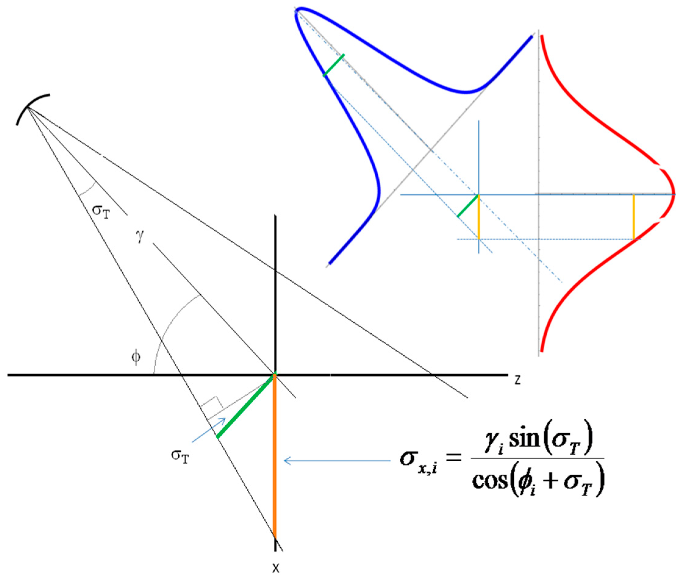
which is the subtended angle of each mirror i in the plane XY with respect to the x axis. The values of σ_x,i [cm] and σ_y,i [cm] are defined by the projection of the circular Gaussian distribution on the plane XY and are given by

$${\sigma }_{x,i}={\displaystyle \frac{{\gamma }_i\sin \left({\sigma }_T\right)}{\cos \left({\varphi }_i+{\sigma }_T\right)}}$$

(28)

$${\sigma }_{y,i}={\gamma }_i\tan \left({\sigma }_T\right)$$

(29)

Notice that σ_x,i is obtained considering the distance γ_i and the angle ϕ_i as shown in Figure 9. On the other hand, σ_y,i only depends on the distance γ_i.

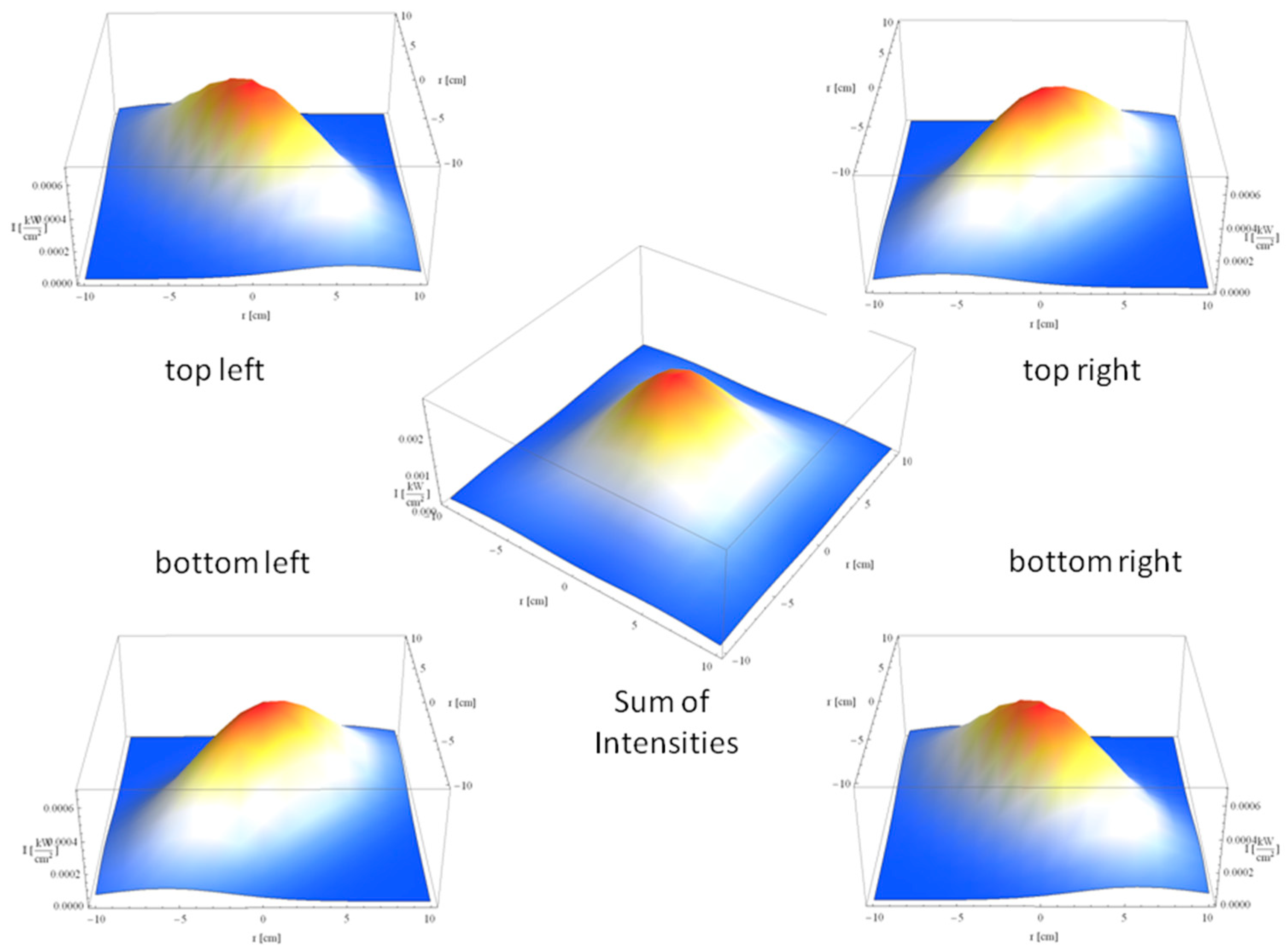
The total energy distribution at the focal point of the HRFSF is derived by summing the elliptical Gaussian distributions produced by each mirror, in accordance with the superposition principle of radiation, while disregarding non-linear effects. The overlap of these distributions creates the focal spot of the concentrator. As illustrated in Figure 10, four symmetrically arranged mirrors generate a well-defined elliptical Gaussian pattern, which, when superimposed, is effectively represented by the Gaussian distribution shown in the center of the figure.

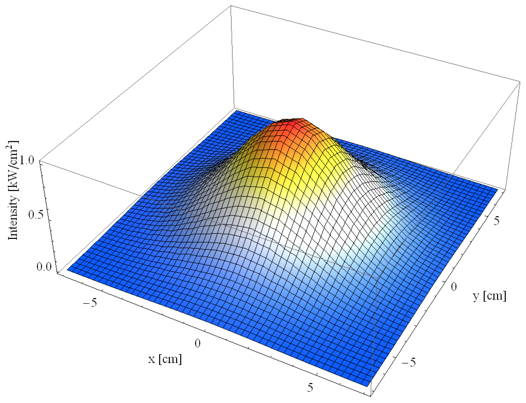
Therefore, the total intensity distribution on the spot can be written as

$$G_{T,\hspace{0.17em}xy}=Q_s\hspace{0.17em}{\displaystyle \sum }_{i=1}^{409}{\displaystyle \frac{\left(\exp \left(-\left({\phi }_i{x}^2+2{\kappa }_{i}xy+{\lambda }_i{y}^2\right)\right)\right)}{2\pi {\sigma }_{x,\hspace{0.17em}i}{\sigma }_{y,\hspace{0.17em}i}}}$$

(30)

The analysis of the added effect from the 409 mirrors of the furnace reveals that the distribution approximates a Gaussian shape, as illustrated in Figure 11. To quantitatively assess this phenomenon, Equation (30) was numerically evaluated utilizing the Mathematica Software™. The resulting values were subsequently fitted to an elliptical Gaussian distribution, highlighting the precision and effectiveness of the methodological approach.

$$G_{T,\hspace{0.17em}xy}={\displaystyle \frac{Q_s}{2\pi {\sigma }_x{\sigma }_y}}\left(\exp \left(-{\displaystyle \frac{1}{2}}\left({\left({\displaystyle \frac{x}{{\sigma }_x}}\right)}^2+{\left({\displaystyle \frac{y}{{\sigma }_y}}\right)}^2\right)\right)\right)$$

(31)

The values of σ_x and σ_y are found to be:

$$\begin{array}{c}{\sigma }_x=2.51\hspace{0.17em}\mathrm{cm}\\ {\sigma }_y=2.50\hspace{0.17em}\mathrm{cm}\end{array}$$

Considering that Q_s can be estimated as:

$$\begin{array}{l}{Q}_s=\left(A_C\right)\hspace{0.17em}\left(q_s\right)\hspace{0.17em}\left({\rho }_h\right)\hspace{0.17em}\left({\rho }_m\right)\\ Q_s=\left(40.06\hspace{0.17em}{\mathrm{m}}^2\right)\hspace{0.17em}\left(1000\hspace{0.17em}{\displaystyle \frac{\mathrm{W}}{{\mathrm{m}}^2}}\right)\hspace{0.17em}\left(0.95\right)\hspace{0.17em}\left(0.95\right)=36.16\hspace{0.17em}\mathrm{kW}\end{array}$$

the peak concentration can be calculated by

$$\begin{array}{c}Peak={\displaystyle \frac{Q_s}{2\pi {\sigma }_x{\sigma }_y}}=9171.6\hspace{0.17em}{\displaystyle \frac{\mathrm{kW}}{{\mathrm{m}}^2}}\\ =0.91716\hspace{0.17em}{\displaystyle \frac{\mathrm{kW}}{{\mathrm{cm}}^2}}\end{array}$$

The concentrated solar flux distribution G_T,xy on the spot of the concentrator is shown in Figure 11.

If it is considered that the integral in 2D of G_T,xy in the intervals −2σ_x ≤ σ_x ≤ 2σ_x, and −2σ_y ≤ σ_y ≤ 2σ_y, it is expected that 92% of the radiant energy will be contained in the spot, namely,

$$Q{s}_{92\%}={\displaystyle \frac{Q_s}{2\pi {\sigma }_x{\sigma }_y}}{\int }_{-2{\sigma }_y}^{2{\sigma }_y}{\int }_{-2{\sigma }_x}^{2{\sigma }_x}\left(\exp \left(-{\displaystyle \frac{1}{2}}\left({\left({\displaystyle \frac{x}{{\sigma }_x}}\right)}^2+{\left({\displaystyle \frac{y}{{\sigma }_y}}\right)}^2\right)\right)\right)\hspace{0.17em}dxdy=32.94\hspace{0.17em}\mathrm{kW}$$

(32)

On the other hand, the shape of the spot is an ellipse described by

$$\begin{array}{cc}\hfill {\left({\displaystyle \frac{x}{a_1}}\right)}^2+{\left({\displaystyle \frac{y}{b_1}}\right)}^2& =1\hfill \\ \hfill a_1& =2{\sigma }_x=5.02\hspace{0.17em}\mathrm{cm}\hfill \\ \hfill b_1& =2{\sigma }_y=5.00\hspace{0.17em}\mathrm{cm}\hfill \end{array}$$

(33)

And the area of the spot is therefore

$$A_{spot}=\pi \left(2{\sigma }_x\right)\hspace{0.17em}\left(2{\sigma }_y\right)=78.84\hspace{0.17em}{\mathrm{cm}}^2$$

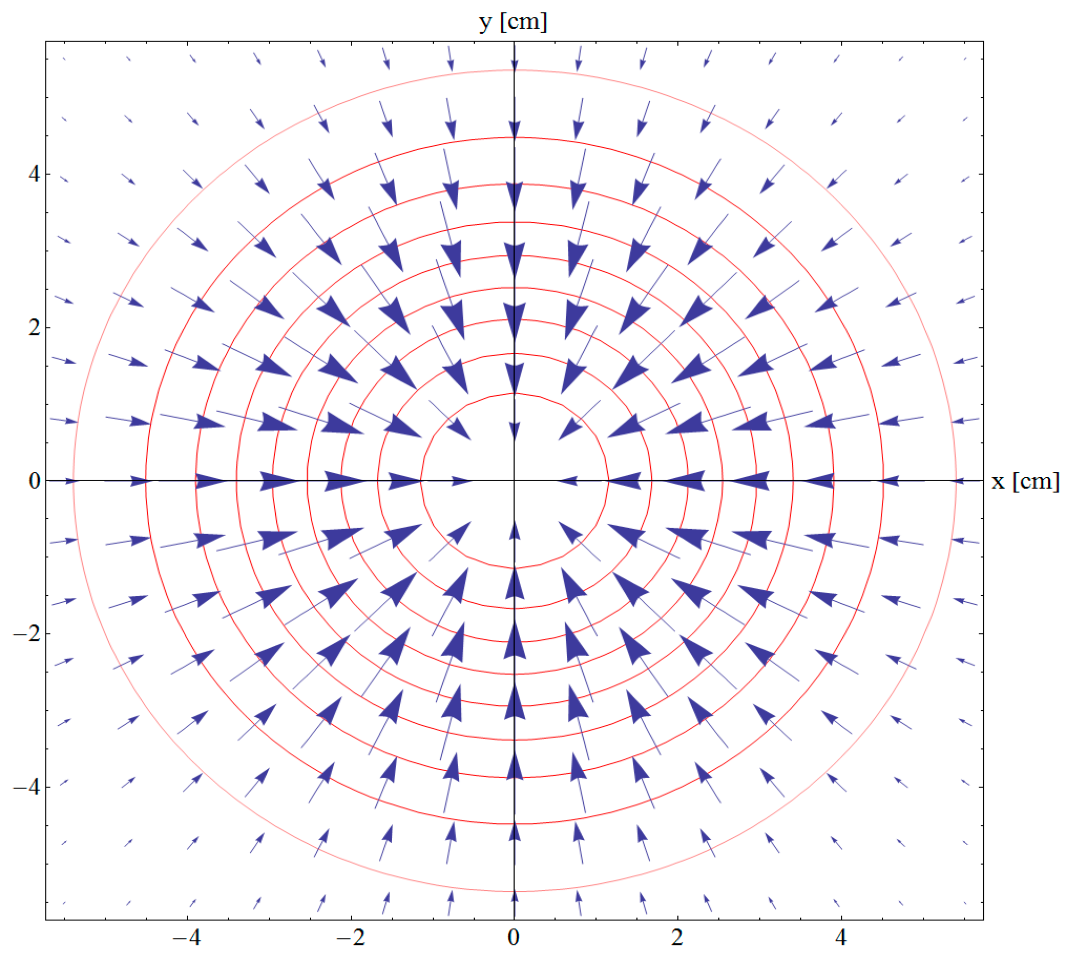
Based on the proposed concentrated solar flux distribution in Equation (31), the isocontour shapes can be obtained in 2D. The isocontours are the contour lines with constant irradiance (power per unit of area), and can be calculated by equating G_T,xy in Equation (31) to a constant.

$$\begin{array}{cc}\hfill {\displaystyle \frac{Q_s}{2\pi {\sigma }_x{\sigma }_y}}\left(\exp \left(-{\displaystyle \frac{1}{2}}\left({\left({\displaystyle \frac{x}{{\sigma }_x}}\right)}^2+{\left({\displaystyle \frac{y}{{\sigma }_y}}\right)}^2\right)\right)\right)& =nCte\hfill \\ \hfill {\displaystyle \frac{Q_s}{2\pi {\sigma }_x{\sigma }_y}}& =Cte\hfill \\ \hfill 0& <n<1\hfill \end{array}$$

(34)

In Equation (34) it is assumed that the value of the constant is between n < 0, and the peak value of the function n < 1. This way, it is easy to show that the level curves are ellipses, as depicted by Equation (35).

$$\begin{array}{cc}\hfill \exp \left(-{\displaystyle \frac{1}{2}}\left({\left({\displaystyle \frac{x}{{\sigma }_x}}\right)}^2+{\left({\displaystyle \frac{y}{{\sigma }_y}}\right)}^2\right)\right)& =n\hfill \\ \hfill {\left({\displaystyle \frac{x}{2{\sigma }_x}}\right)}^2+{\left({\displaystyle \frac{y}{2{\sigma }_y}}\right)}^2& =\ln \left({\displaystyle \frac{1}{n}}\right)\hfill \\ \hfill {\left({\displaystyle \frac{x}{a_2}}\right)}^2+{\left({\displaystyle \frac{y}{b_2}}\right)}^2& =1\hfill \\ \hfill a_2& =2{\sigma }_x\ln \left({\displaystyle \frac{1}{n}}\right)\hfill \\ \hfill b_2& =2{\sigma }_y\ln \left({\displaystyle \frac{1}{n}}\right)\hfill \end{array}$$

(35)

In this context, each ellipse is characterized by the parameters a₂ and b₂, which vary with the distances defined by the variables x and y, as well as a specific value of n. This relationship underscores the geometric properties of the ellipses, facilitating their analysis within various mathematical and physical frameworks.

Moreover, with Mathematica, it is possible to obtain the plot of the gradient $\nabla G_{T,\hspace{0.17em}xy}$ of the scalar field defined by Equation (31). This is the vector field pointing in the direction of the steepest increase $G_{T,\hspace{0.17em}xy}$ at every point, and whose magnitude is the rate of change in that direction.

$$\begin{array}{l}\nabla G_{T,\hspace{0.17em}xy}={\displaystyle \frac{Q_s}{2\pi {\sigma }_x{\sigma }_y}}\nabla \left(\left(\exp \left(-{\displaystyle \frac{1}{2}}\left({\left({\displaystyle \frac{x}{{\sigma }_x}}\right)}^2+{\left({\displaystyle \frac{y}{{\sigma }_y}}\right)}^2\right)\right)\right)\right)\\ \nabla G_{T,\hspace{0.17em}xy}=\left({\displaystyle \frac{\partial G_T}{\partial x}},\hspace{0.17em}{\displaystyle \frac{\partial G_T}{\partial y}}\right)\\ \nabla G_{T,\hspace{0.17em}xy}=\left[{\displaystyle \frac{Q_s}{2\pi {\sigma }_x{\sigma }_y}}\exp \left(-{\displaystyle \frac{1}{2}}\left({\displaystyle \frac{x^2}{{\sigma }_x^2}}+{\displaystyle \frac{y^2}{{\sigma }_y^2}}\right)\right)\right]\hspace{0.17em}\left(-{\displaystyle \frac{x}{{\sigma }_x^2}},-{\displaystyle \frac{y}{{\sigma }_y^2}}\right)\end{array}$$

(36)

In Figure 12 some level curves for the spot of the concentrator and the gradient vector field are depicted.

7. Analytic Model of the Solar Flux Distribution in 3D

An analytical equation describing the energy distribution at a specific point in three-dimensional space can be derived by analyzing the focal region of the solar furnace. The methodology established for determining the distribution in the XY plane can be adapted for the XZ or YZ planes. For instance, when the YZ plane is focused on, the variable x should be replaced with z, necessitating modifications to Equations (27) and (28) accordingly.

$${\theta }_{yz,\hspace{0.17em}i}=\arccos \left({\displaystyle \frac{z_i}{\sqrt{z_i^2+y_i^2}}}\right)$$

(27′)

and

$${\sigma }_{z,\hspace{0.17em}i}={\displaystyle \frac{{\gamma }_i\sin \left({\sigma }_T\right)}{\sin \left({\phi }_i+{\sigma }_T\right)}}$$

(28′)

It’s important to note that formulas (27’) and (28’) reflect the same calculations as the earlier formulas (27) and (28), with the only difference being the substitution of x with z. Once the previous procedure has been carried out, the values of σ_z and σ_y are, respectively,

$$\begin{array}{c}{\sigma }_z=3.55\hspace{0.17em}\mathrm{cm}\\ {\sigma }_y=2.50\hspace{0.17em}\mathrm{cm}\end{array}$$

Note that the value for σ_y must be recovered in this new procedure.

The equation that describes energy by unit of time and unit of volume at the spot on the concentrator is

$$G_{T,\hspace{0.17em}xyz}={\displaystyle \frac{Q_s}{2\pi {\sigma }_x{\sigma }_y{\sigma }_z}}\left(\exp \left(-{\displaystyle \frac{1}{2}}\left({\left({\displaystyle \frac{x}{{\sigma }_x}}\right)}^2+{\left({\displaystyle \frac{y}{{\sigma }_y}}\right)}^2+{\left({\displaystyle \frac{z}{{\sigma }_z}}\right)}^2\right)\right)\right)$$

(37)

In a manner analogous to the two-dimensional case, it is possible to derive the isosurfaces’ shapes within three-dimensional space. The isosurfaces correspond to regions where the variable of interest maintains a constant value per unit area. To compute these surfaces, one can set Equation (37) equal to a constant, thereby identifying the specific locations in the 3D space where this condition holds true. This method facilitates a comprehensive visualization of the spatial distributions of the measured quantity,

$$\begin{array}{cc}\hfill {\displaystyle \frac{Q_s}{2\pi {\sigma }_x{\sigma }_y{\sigma }_z}}\left(\exp \left(-{\displaystyle \frac{1}{2}}\left({\left({\displaystyle \frac{x}{{\sigma }_x}}\right)}^2+{\left({\displaystyle \frac{y}{{\sigma }_y}}\right)}^2+{\left({\displaystyle \frac{z}{{\sigma }_z}}\right)}^2\right)\right)\right)& =nKte\hfill \\ \hfill {\displaystyle \frac{Q_s}{2\pi {\sigma }_x{\sigma }_y{\sigma }_z}}& =Kte\hfill \\ \hfill 0& <n<1\hfill \end{array}$$

(38)

The level surfaces are ellipsoids that are described by Equation (39),

$$\begin{array}{cc}\hfill {\left({\displaystyle \frac{x}{a_3}}\right)}^2+{\left({\displaystyle \frac{y}{b_3}}\right)}^2+{\left({\displaystyle \frac{z}{c_3}}\right)}^2& =1\hfill \\ \hfill a_3& =2{\sigma }_x\ln \left({\displaystyle \frac{1}{n}}\right)\hfill \\ \hfill b_3& =2{\sigma }_y\ln \left({\displaystyle \frac{1}{n}}\right)\hfill \\ \hfill c_3& =2{\sigma }_z\ln \left({\displaystyle \frac{1}{n}}\right)\hfill \end{array}$$

(39)

The gradient of a scalar field of Equation (37) is calculated as

$$\begin{array}{l}\nabla G_T={\displaystyle \frac{Q_s}{2\pi {\sigma }_x{\sigma }_y{\sigma }_z}}\nabla \left(\left(\exp \left(-{\displaystyle \frac{1}{2}}\left({\left({\displaystyle \frac{x}{{\sigma }_x}}\right)}^2+{\left({\displaystyle \frac{y}{{\sigma }_y}}\right)}^2+{\left({\displaystyle \frac{z}{{\sigma }_z}}\right)}^2\right)\right)\right)\right)\\ \nabla G_T=\left[{\displaystyle \frac{Q_s}{2\pi {\sigma }_x{\sigma }_y{\sigma }_z}}\exp \left(-{\displaystyle \frac{1}{2}}\left({\displaystyle \frac{x^2}{{\sigma }_x^2}}+{\displaystyle \frac{y^2}{{\sigma }_y^2}}+{\displaystyle \frac{z^2}{{\sigma }_z^2}}\right)\right)\right]\hspace{0.17em}\left(-{\displaystyle \frac{x}{{\sigma }_x^2}},-{\displaystyle \frac{y}{{\sigma }_y^2}},-{\displaystyle \frac{z}{{\sigma }_z^2}}\right)\end{array}$$

(40)

In Figure 13, a representation of various level surfaces associated with the three-dimensional configuration of the concentrator is presented, alongside the corresponding gradient vector field. This illustration effectively demonstrates the spatial relationships and directional tendencies inherent within the system.

To determine the sensitivity of the analytical model,

Table 3. Sensitivity analysis of the analytical model.

Metric	Minimum Values σs = 3.6 mrad σFacets, = σHeliostat = σTracking = 1.0 mrad	This Model σs = 4.47 mrad σFacets, = 1.0 mrad σHeliostat = 2.0 mrad σTracking = 2.0 mrad	Maximum Values σs = 5.64 mrad σFacets, = σHeliostat = σTracking = 2.0 mrad
Spot Radius (cm)	3.71	5.01	6.14
Peak Flux (kW/m2)	16,663.7	9171.64	7637.8
Mean Concentration (kW/m2)	9230.5	5081.24	3331.5

presents the peak flux and spot size, considering the solar brightness distribution modeled as a Gaussian distribution, ranging from 3.6 mrad to 5.64 mrad. The minimum values for σ_Facets, σ_Heliostat, and σ_Tracking are set at 1.0 mrad, while the maximum values are established at 2.0 mrad for each parameter.

In the following section, the validation of both the 2D and 3D models is presented, referencing two papers [20,21,22] from the literature. These papers discuss a comprehensive theoretical ray tracing method and an experimental analysis of solar concentration profiles for the high radiative solar furnace located at IER-UNAM in Temixco, Mexico.

8. Validation of the 2D and 3D Models

To validate the two-dimensional analytical model developed in this research, the results obtained were compared with those reported by Estrada et al. [21]. Their study provides a comprehensive methodology for determining and validating solar concentration profiles in the high-radiative solar furnace at UNAM. The research consists of two complementary phases: experimental and analytical. In the experimental phase, an 81 m² heliostat was used to focus solar radiation onto a concentrator made up of 409 precisely aligned facets. A range of measurement devices was utilized, including a CCD camera for capturing images of the sunspot, a Gardon^® radiometer to measure irradiance at the focal point, and a Lambertian target employed in concentrated solar systems to assess the spatial distribution and intensity of solar flux. A Lambertian target is a surface that uniformly reflects incident light in all directions, regardless of the angle of incidence. This characteristic ensures that the observed radiance (brightness) remains consistent from any viewing angle. As a result, it functions as both a calibration and measurement tool, effectively capturing the true intensity profile of focused sunlight and facilitating accurate flux mapping.

During the analytical phase, ray tracing techniques were implemented using the Tonalli program to simulate the system’s optical behavior. The solar flux distribution in the focal plane was modeled using convolution methods, assuming a two-dimensional Gaussian distribution to account for global optical errors. The evaluation of the facets, the tracking system, and the optical aberrations related to the heliostat was performed using both empirical measurements and computational analyses. The outcomes of this assessment have been documented in references [21,22].

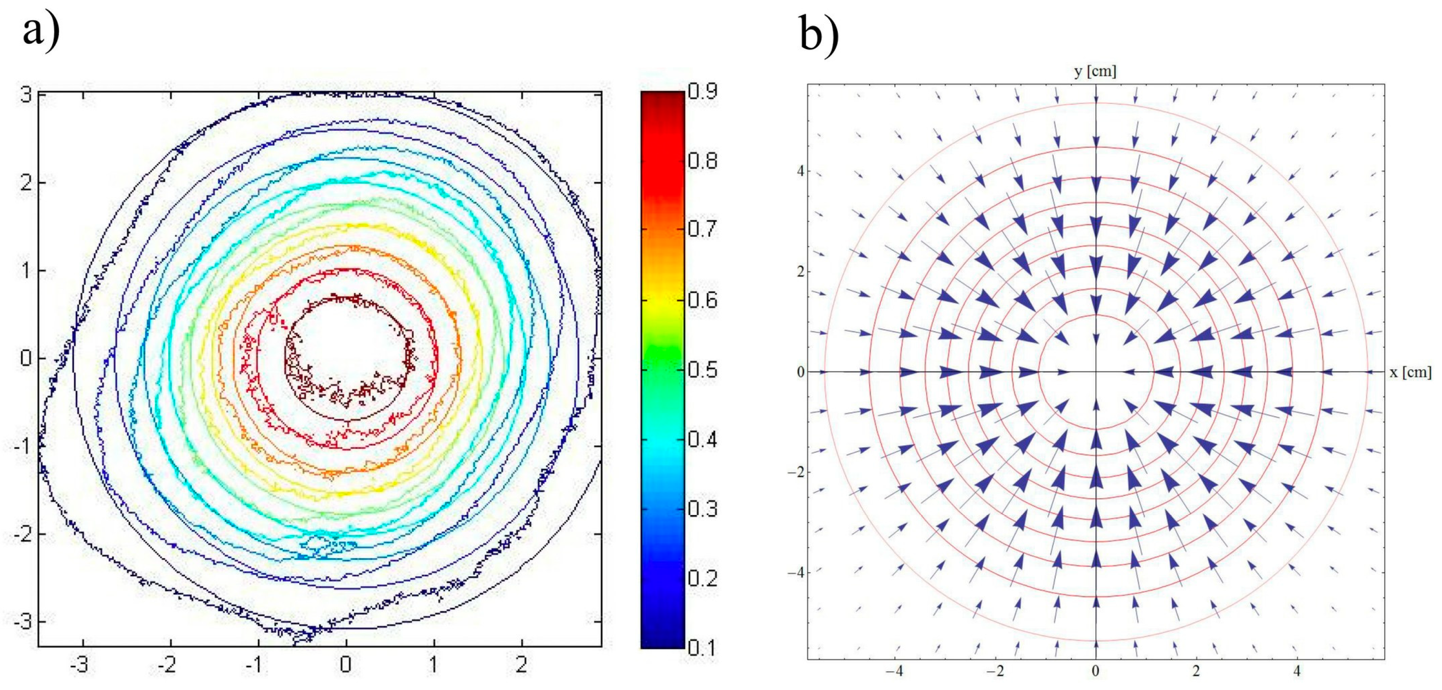
In Figure 14, the outcomes reported in [21] are compared with those of the present study. This comparison clearly shows that the simple analytical model developed here is supported by both the experimental results and the ray tracing method. This validation highlights the robustness and reliability of the proposed model in capturing the relevant phenomena.

To validate the three-dimensional analytical model, the results presented by Prez-Enciso et al. [22] were considered. Their study aimed to characterize the spatial distribution of concentrated solar radiation in the furnace’s focal zone by integrating ray tracing simulations with direct experimental measurements. During the experimental phase, a Lambertian screen was positioned at the focal point, and images of the concentrated solar flux were captured using an 8-bit CCD camera. These images, along with irradiance profiles obtained at 5 mm intervals over a 10 cm span along the optical axis, were processed using MATLAB^® to extract quantitative flux distributions. At the same time, ray tracing simulations were conducted with SOLTRACE to generate theoretical flux profiles

Figure 15 compares the results from [22] with those obtained in this study side by side. This comparison clearly shows that the straightforward analytical model developed here is backed by both the experimental data and the results of ray tracing simulations. Such validation emphasizes the model’s robustness and reliability in effectively capturing crucial phenomena.

Table 4. Comparison of peak flux, spot size, and non-uniformity values among the analytical model, experiments, and ray tracing simulations.

Metric	Analytical Model σs = 4.47 mrad σFacets, = σHeliostat = σTracking = 1.0 mrad	Ray Tracing [21,22]	Experiment [21,22]	Relative Error × 100% $\frac{\left|{\mathit{V}}_{\mathit{m}\mathit{o}\mathit{d}\mathit{e}\mathit{l}}-{\mathit{V}}_{\mathit{e}\mathit{x}\mathit{p}.}\right|}{{\mathit{V}}_{\mathit{e}\mathit{x}\mathit{p}.}}$
Spot Radius (cm)	4.46	4.9	4.6 ± 0.1	3.04%
Peak Flux (kW/m2)	11,565.6	10,000	11,838	2.30%
Mean Concentration (kW/m2)	5497.4	5000	5792	5.09%

compares peak flux, spot size, and non-uniformity values among the analytical model, experimental data, and ray tracing simulation results. By analyzing these parameters across the different methodologies, we can identify the strengths and limitations of each approach, ultimately contributing to a more robust understanding of the underlying phenomena.

In the subsequent section, the primary conclusions derived from this research are presented.

9. Conclusions

The primary conclusions derived from the research are delineated below.

• This study finds that the sunshape affects the distribution of concentrated solar flux in high-flux solar furnaces. Using Gaussian approximation, the developed model effectively describes the radial energy profile of the sun, thereby simplifying calculations without compromising accuracy.
• The measurement system established in this research enables a detailed characterization of the sun’s angular brightness profile, improving our understanding of its implications for solar concentration systems.
• The CCD Circumsolar Scope (CCS) has been validated as an effective tool for capturing high-resolution solar imagery and analyzing the sunshape under various atmospheric conditions. The measurement campaign produced a substantial dataset that significantly enhances the accuracy of the sunshape model, ensuring that variations in solar brightness and circumsolar radiation are thoroughly considered in the analysis of solar flux distribution.
• The analytical model developed here successfully approximates the solar brightness distribution using a Gaussian function. The results show that this methodology provides a computationally efficient way to simulate the sunshape while maintaining the essential characteristics needed for accurate solar flux distribution modeling.
• This model is adaptable to varying atmospheric conditions, thus reinforcing its relevance to solar energy research.
• By integrating the sunshape model with the optical inaccuracies associated with the heliostat, mirrors, and tracking systems, this study defines an effective solar source for the solar furnace. The results indicate that the convolution of these effects produces a Gaussian-like distribution, which can significantly enhance the precision of solar flux predictions and improve the design of solar furnaces.
• The geometric optics model employed in this investigation proficiently predicts the concentration ratio of the High-Radiative Flux Solar Furnace (HRFSF). The findings reveal the crucial effects of mirror positioning, curvature, and focal distance on overall concentration performance.
• The analytical approach provided herein serves as a dependable method for estimating flux distribution, while minimizing the necessity for extensive computational resources.
• This study establishes that the total solar flux distribution at the focal plane can be effectively represented as a summation of elliptical Gaussian distributions emanating from each mirror. The resulting intensity distribution closely correlates with empirical observations, thereby validating the accuracy of the model.
• Further analyses of level curves and gradient vector fields enhance the understanding of flux distribution patterns.
• This research successfully derives an analytical equation that outlines the spatial distribution of solar flux within the focal region by extending the 2D model into a three-dimensional framework, resulting in an equation that describes the volumetric distribution of solar flux, including its isosurfaces and gradient fields.
• The 3D model effectively captures the spatial flux distribution in the focal region, providing a comprehensive view of the system’s behavior.
• Additionally, the analytical predictions in both 2D and 3D are compared with experimental results and ray tracing simulations from the literature, showing a strong agreement between the proposed models and the validated data, confirming the accuracy and robustness of the developed analytical approach.
• Overall, this study’s analytical methodology efficiently and precisely estimates solar flux distribution in high-flux solar furnaces. The Gaussian approximation is demonstrated to be a robust approach that balances computational efficiency with accuracy.
• Incorporating optical error analysis further refines the model’s applicability to real-world solar furnace systems.
• Collectively, these findings advance the field of solar energy research by providing a reliable alternative to intricate ray tracing simulations, which is particularly beneficial for preliminary design evaluations and system optimization.

Overall, this study’s analytical methodology efficiently and precisely estimates solar flux distribution in high-flux solar furnaces. The Gaussian approximation is demonstrated to be a robust approach that balances computational efficiency with accuracy. Incorporating optical error analysis further refines the model’s applicability to real-world solar furnace systems. Collectively, these findings advance the field of solar energy research by providing a reliable alternative to intricate ray tracing simulations, which is particularly beneficial for preliminary design evaluations and system optimization.