Abstract
Atmospheric pollution results from toxic gases in low concentrations, originating from natural processes and human activities. These gases interact with each other in the presence of solar radiation, forming much more complex compounds that contribute to the formation of photochemical smog. This study presents a mathematical model to estimate the daily concentrations of primary and secondary pollutants, assuming that spatial variation is not considered within a control volume. The model includes nitrogen oxides, ozone, hydrocarbons, aldehydes, alcohols, and other gases, which are related through 52 chemical and photochemical reactions with rate constants that depend on factors such as the time of day and temperature. The model formulation results in 31 ordinary differential equations that are solved using a variable-step algorithm in MATLAB R2019a. Two scenarios are simulated: the “closed-box” model (CBM), where there are no inflows or outflows of gaseous flux, and the “open-box” model (OBM), which includes inflows and outflows within the control volume. The OBM is particularly useful for predicting concentrations during thermal inversion episodes. The results show that several pollutants reach their maximum concentrations at midday, suggesting an increase in the formation of secondary pollutants under high solar radiation, especially in the closed-box model. In the open-box model, concentration peaks shift toward the afternoon. To compare both models, the closed-box system conditions are considered, incorporating airflow into the open-box model without accounting for pollutants transported by this flow. The complex nonlinear dynamics observed in the pollutants highlight the combined influence of solar radiation, temperature, and emission rates on air quality. This study underscores the usefulness of mathematical models in developing effective mitigation strategies and assessing environmental and public health impacts.
1. Introduction
The lower atmosphere, known as the troposphere, is a continuous source of pollution due to the emission of primary pollutants such as nitrogen oxides (), carbon monoxide (), and volatile organic compounds (VOCs). These substances originate naturally and from human activities, including vehicular traffic, industry, and the use of fossil fuels; a study by the National University of San Marcos, Lima, Peru, indicates that transportation contributes 70% of carbon monoxide emissions and 40% of nitrogen oxides emissions in the city. Studies conducted by the Technological University of Peru and the Private University of the North report that the paint industry and fuel marketing centers are sources of volatile organic compounds. Under favorable environmental conditions and solar radiation, these compounds can transform into a series of secondary pollutants, among which tropospheric ozone () stands out due to its adverse effects on human health and ecosystems [1].
Air pollution is one of the most pressing environmental issues globally. It has significant impacts on climate change and public health, increasing both morbidity and mortality rates [2]. For this reason, the reaction mechanisms proposed in the literature have focused their analyses on processes primarily involving nitrogen oxides, VOCs, and ozone, among others. For the determination of some primary pollutants such as hydrocarbons and soot particles, Raman spectroscopy is used, standing out for its precision and simultaneous analysis capability [3,4,5]. Using adsorption and oxidation techniques, a high percentage of and can be removed from a gas mixture [6,7].
Tropospheric ozone, a secondary pollutant, is primarily formed through photochemical reactions in the presence of and VOCs. Its concentration is strongly correlated with these precursors and other meteorological factors such as solar radiation, temperature, and wind speed [8]. This pollutant is responsible for an increased incidence of cardiovascular and respiratory diseases and negatively impacts agricultural crops and natural ecosystems [9]. Tropospheric ozone responds almost directly to changes in atmospheric conditions and the concentrations of its precursors. Forecasting models have been developed to predict its concentrations within 24 h, enabling more precise planning for mitigating its effects [10]. A study on climate change and future tropospheric ozone concentrations in the Northern Hemisphere highlighted an increase in ozone exchange between the stratosphere and troposphere (STE) in Europe and eastern China, reinforcing the need for appropriate environmental policies [11]. Another study identified temperature as the dominant factor, explaining approximately 40% of annual ozone concentrations, and emphasized the interaction between multiple meteorological factors that significantly impact ozone levels, especially during summer [12].
Between 2020 and 2022, the impact of tropospheric ozone on 20 rice varieties in Bangladesh was evaluated. The use of ethylenediurea (EDU) increased grain yield by an average of 10.4%, highlighting the negative effect of ozone on agricultural production [13]. During the COVID-19 pandemic, an improvement in air quality was observed, along with a positive correlation between levels and COVID-19 cases, suggesting that pollution could increase the risk of infection and mortality [14]. The reduction in ozone-depleting substances has decreased ultraviolet (UV) radiation at the surface, improving air quality; however, climate change may alter these effects in the future [15,16].
Urban air quality has been studied with a focus on ozone () concentration and its formation, influenced by both photochemical processes and the transport of precursors such as from industrial areas. Despite reductions in and volatile organic compounds, levels have remained high, indicating a nonlinear relationship with its precursors and the need for more effective mitigation strategies [17].
In northern China and the Pearl River Delta, under specific meteorological conditions such as static stability and the diurnal cycle of the mixing layer, an explosive increase in was observed, highlighting the complex interaction between meteorology and air quality [18]. Globally, tropospheric ozone has increased since the 20th century, driven by anthropogenic factors and meteorological conditions such as anticyclones and sea breezes, which affect its transport and dispersion. This suggests that reducing does not always guarantee a decrease in , emphasizing the need for targeted policies for its control [19,20]. Furthermore, photochemical smog, composed of ozone and other secondary pollutants such as acids and peroxides, has been identified as primarily originating from nitrogen oxides and volatile organic compounds [21].
Other pollutants hazardous to human health and the environment include and , whose increase is attributed to fires, industrial activity, and other causes [22]. In areas with low industrial activity, the concentration of these two pollutants is significantly lower [23].
Mathematical modeling is widely applied to assess the impact of air pollutants on human and ecological health, considering factors such as emission sources (both natural and anthropogenic), meteorology (topography, temperature, wind currents), and chemical processes (reactions, aerosol formation, sinks) [2,24,25,26]. Various studies have compared numerical schemes for predicting air quality in urban areas. For example, a study on the cities of Los Angeles and Philadelphia found that the Zalesak method predicts ozone peaks more accurately than the SHASTA method in Los Angeles, while in Philadelphia, the differences are minimal [27]. Additionally, the modular SSH-aerosol model is presented, which simulates the evolution of gases and aerosols, improving prediction accuracy in urban areas through the use of computational fluid dynamics (CFD) software such as OpenFOAM [28].
Several mathematical modeling strategies were reviewed, including Gaussian, Lagrangian, and Eulerian models, together with CFD, highlighting their advantages and disadvantages along with advancements in parallel computing and adaptive mesh refinement [24,29,30,31]. Furthermore, an analytical solution for atmospheric pollutant dispersion was introduced using a fractional approach, which outperforms traditional solutions by considering memory effects in turbulence [32]. A study developed a mathematical model for industrial emission dispersion, incorporating factors such as the deposition velocity of fine particles and utilizing a second-order implicit finite difference scheme, demonstrating high accuracy when compared with field data [33]. The main limitation of these models is their reliance on Gaussian dispersion schemes, which omit chemical and photochemical reactions. Including such reactions would result in an immense number of differential equations, leading to implementation and convergence challenges.
One of the challenges before simulating pollutant dispersion is standardizing data for second-order reaction rate constants, as they are reported in various units. Atkinson et al. proposed a conversion table to address this issue and presented kinetic data on second- and third-order chemical and photochemical reactions [34]. Key mechanisms involved in these reactions include nitrogen oxides, ozone, atomic oxygen, hydrogen peroxide, and radicals such as hydroperoxide and hydroxyl [35,36].
A study conducted in India analyzed the temporal concentrations of gases such as , , and from January 2017 to December 2020, showing diurnal peaks for and , while reached its maximum at midday [37]. Additionally, an analytical solution for pollutant dispersion was presented, based on a three-dimensional, fractional-order advection–diffusion equation, which demonstrated better parameterization compared to Gaussian models, emphasizing the superiority of fractional-order derivatives in predictions [32].
A study on pollution in the Beijing–Tianjin–Hebei region analyzed haze control using a diffusion model based on the Gaussian plume. It concluded that industrial emissions were the primary source of , with higher concentrations near emission sources, and that atmospheric stability was greater in autumn and winter, which is crucial for formulating effective environmental regulations [38]. In Tulsa, ozone modeling was conducted using neural networks, improving accuracy by incorporating past meteorological ozone data, achieving a correlation of 0.88 with atmospheric data, making it suitable for use in automated forecasting systems [39].
The mechanism and transformation of primary pollutants such as nitrogen oxides (), volatile organic compounds (VOCs), and sulfur dioxide () into secondary pollutants like ozone () and aerosols, as well as the formation of photochemical smog and tropospheric chemistry, are explained through chemical and photochemical reactions in the troposphere [40]. The transformation of primary pollutants into secondary pollutants such as ozone and aerosols through sunlight-driven reactions is further detailed in studies [41,42].
The WRF-Chem (Weather Research and Forecasting with Chemistry) model integrates meteorological components with chemical and photochemical processes in the atmosphere. It is used to simulate the formation and dispersion of secondary pollutants at regional and global scales. The model is widely applied in research on tropospheric ozone, aerosols, and other secondary pollutants [43]. The EMEP (European Monitoring and Evaluation Programme) employs atmospheric chemistry models to study primary and secondary pollutants at the regional level in Europe. EMEP models simulate chemical and photochemical processes, particularly those affecting the formation of ozone and aerosols. They focus on the interaction between pollutants emitted from human sources and their transformations in the atmosphere [44].
The GEOS-Chem model is a global atmospheric chemistry model that simulates the formation and distribution of primary and secondary pollutants. It is widely used to study the effects of photochemical chemistry on ozone and aerosol formation, including the interaction between and VOCs in the production of tropospheric ozone and fine particulate matter (PM2.5) [45].
The CAMx (Comprehensive Air Quality Model with Extensions) is an air quality model that incorporates both chemical and photochemical processes. It predicts the concentrations of primary and secondary pollutants, such as ozone and aerosols, and is used for regional-scale studies to address air pollution issues [46].
Kinetic data on the reaction rate constants for each component involved in photochemical smog formation are presented in some cases as a function of temperature, while in others, they are provided independently of temperature for first-, second-, and third-order kinetics [34].
A simplified resolution technique proposes a system of 15 differential equations corresponding to , , , , , , , , , , , , , , and . Assuming a steady-state process, it also includes nine nonlinear algebraic equations for , *, *, , *, *, *, , and . Other components such as *, , , , , , and are not considered in the mathematical development [47].
2. Materials and Methods
Modeling involves identifying, from the relevant literature, the reaction mechanisms of the most common pollutants and their corresponding kinetic constants; one of these mechanisms considers the interaction of 32 chemical species that generate 52 chemical and photochemical reactions. It includes formulating unsteady-state mass balance equations for each component, selecting a transport model coupled with meteorological conditions, and making reasonable assumptions regarding initial conditions and possible emission rates of primary pollutants. While most traditional models are based on the representation of dispersion using Gaussian profiles, the present work adopts the concept of a control volume under an Eulerian approach. This formulation allows a coupled description of transport processes and chemical and photochemical reactions, facilitating their integration into local mass balances within the fluid domain. These elements are fundamental to the present study.
2.1. Mathematical Model
The mathematical modeling framework for the chemical and photochemical processes in the “closed-box” model is presented, focusing on a period of thermal inversion. In this scenario, kinetic parameters are required, including indirect solar radiation for photochemical reactions, along with initial concentrations and emission rates.
For the “open-box” model, under the same conditions as the closed-box model, additional parameters must be considered, such as altitude above sea level and thermal inversion height (stable atmosphere), which allow for the calculation of density and pressure. Using knowledge of the geometric dimensions of the control volume, the air inflow and outflow can be determined, along with the respective pollutant concentrations.
Figure 1 illustrates the corresponding modeling scheme for the chemical and photochemical interactions of tropospheric pollutants, considering mixing within the control volume. This volume is bounded at the top by the thermal inversion layer, while its width and length are determined by geographical conditions or arbitrarily set limits.
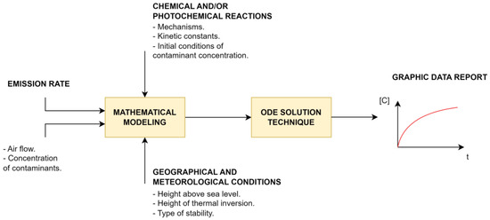
Figure 1.
Modeling the process of tropospheric pollutant dynamics in an open-box model.
2.2. Reaction Mechanism
In the literature, various reaction mechanisms are found, ranging from those composed of a few chemical and photochemical reactions to highly complex mechanisms involving a series of chemical substances. Bazzel reports a reaction mechanism consisting of 7 photochemical reactions involving nitrogen oxides, ozone, nitrous acid, and formaldehyde, among others, whose constants depend on the solar zenith angle [48]; mechanisms for the formation and chemical and photochemical decomposition of bromine compounds have been proposed to understand the distribution of as a function of the atmospheric column height [49]. A mechanism consisting of 65 chemical and photochemical reactions is described by Hampson and Garvin, 1977 [50], which involves the chemical and photochemical interactions of primary and secondary pollutants. A reaction mechanism consisting of 217 chemical equations is presented by Leone and Seinfeld, 1985 [51]. Another simplified mechanism consisting of 14 chemical and photochemical equations involves air as an energy dissipator and is present in the formation of ozone from monoatomic oxygen and diatomic oxygen [52].
McRae presents kinetic data of a complex mechanism of chemical and photochemical interactions in the atmosphere, composed of a system of 52 chemical equations, whose resolution applies a hybrid method of 15 ordinary differential equations and 9 nonlinear algebraic equations; it does not take into account 7 components, including water, oxygen, carbon dioxide, hydrogen, monoatomic oxygen in its various forms, the formyl radical, and M (third body) [47,53].
The kinetic model from the literature [47,53,54] is presented below, along with the rate constants of the chemical and photochemical reactions.
- Photolysis of and basic photolytic cycle
- Chemistry of nitrogen trioxide:
- Nitrous acid and peroxy nitrous acid chemistry
- Photolysis of nitrous acid:
- Nitrous acid chemistry
- Conversion of to
- Nitric acid formation:
- Hydroperoxyl radical formation
- Photolysis of ozone
- Photolysis of formaldehyde
- Chemistry of formaldehyde
- Photolysis of higher aldehydes
- Higher aldehyde chemistry
- Olefin chemistry:
- Alkane chemistry:
- Aromatic chemistry
- Alkoxyl radical chemistry
- Photolysis and chemistry of
- Peroxy nitrate chemistry
- Peroxyacyl nitrate chemistry:
- Dinitrogen pentoxide chemistry
- Ozone removal steps
- Ozone wall loss for smog chamber experiments
- Hydrogen peroxide production and photolysis
- Recombination reaction for peroxyalkyl radicals
Most reactions are second order (n = 2). Reactions 1, 10, 14, 20, 21, 22, 24, 34, 35, 41, 43, 45, and 49 are first order (n = 1), while reaction 2 is third order (n = 3). In general, the units are expressed in (ppm1−n min−1). Additionally, the reactions associated with Equations (1), (10), (20)–(22), (24), (35), and (51) correspond to photochemical processes, while the remaining set of equations represents conventional chemical reactions that do not require activation by solar radiation.
The value in smog chambers depends on experimental conditions. On the other hand, Leone and Seinfeld propose the following photochemical equation for ozone decomposition by solar radiation [51].
The rate constant for reactions 39 and 40 are based on the assumption that
The photochemical reaction rate constants are obtained at the time of maximum solar radiation (12:00 hours). For the remaining hours between 06:00 and 18:00, the transformation equation shown in the work of Cutlip and Shacham [55] should be used.
If , then ; otherwise, it takes the following values: , where sign is the sign function, which takes only three values +1, 0, −1, depending on the argument value. The net result is that the rate constant has values only between 06:00 and 18:00 hours and is zero for the other hours. The factor 60 converts the constant expressed in min−1 to h−1.
The respective nomenclature of the molecules and radicals formed during the chemical and photochemical interactions is shown in Table 1.

Table 1.
Nomenclature of chemical species.
Figure 2 schematically illustrates the different relationships between reactants and reaction products.
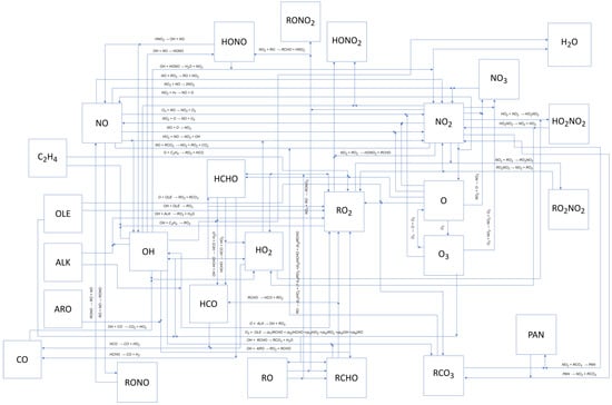
Figure 2.
Photochemical smog formation mechanism consisting of 52 chemical and photochemical [47].
2.3. Mass Transfer Equations Derived from the Reaction Mechanism
The 52 chemical and photochemical reactions described generate 31 differential equations, which allow for calculating the temporal concentrations of the most stable pollutants and short-lived species such as free radicals.
The general form of the global mass balance is given by:
whose integration, after applying Gauss’s Theorem, is:
whose simplification leads to:
Equation (3) is used in the closed-box model by setting and either considering or ignoring the emission rate.
- : Incoming concentration of pollutant i in the control volume, ppm
- : Temporal concentration of pollutant i, ppmv
- : Reaction rate of component i, ppmv/h
- : Emission rate of pollutant i, ppmv/h
- Net volumetric flow of i, ppmv/h
- Residence time, h
The inflow and/or emission of pollutants is considered only for the most important contaminants, such as nitric oxide, alkanes, alcohols, aldehydes, acetylene, etc., while the outflow term is applied to all components. Since oxygen, water vapor, and carbon dioxide are the major constituents, their inflow and outflow terms are nearly equal, making of these components.
In (25), all forms of oxygen are included: monoatomic oxygen, triplet oxygen, and singlet oxygen.
Also considering:
The kinetic components of the convective mass transport equation are represented as a function of the kinetic constants and the respective concentrations, as shown in Table 2.
Table 2.
Kinetic component of the matter conservation equation for each component.
2.4. Atmospheric Parameters
The barometric pressure as a function of altitude above sea level is given by:
- Atmospheric pressure at sea level, 101,325 Pa
- Atmospheric pressure at any altitude
- Adiabatic temperature gradient, 0.0065 K/m
- Temperature at sea level, fluctuating between 273 K and 298 K
- Gravitational acceleration, 9.81 m/s2
- Molecular mass of air, 0.02896 kg/mol
- Universal gas constant, 8.314 J/mol K
- Altitude above sea level, m
- Scale height, m
- Air column height, m
The air pressure as a function of the air column is calculated using:
If we assume that air behaves similarly to an ideal gas:
Replacing (37) in (36):
The integration leads to:
Equation (40) is known as the barometric law. Now, it is necessary to define the parameter H, given by:
Substituting (41) into (40), we obtain the equations for calculating pressure and density in an air column:
Similarly, in the case of air density at a given altitude:
These equations are also used to obtain average values below the thermal inversion zone. With these parameters, it is possible to calculate the residence time of pollutants in a control volume, which is given by:
The volume is calculated based on the geometric dimensions of the control volume:
The flow rate is calculated using
The velocity is obtained from the mass flow velocity
- Mass flow velocity, kg/m2h
- Gas column density, kg/m3
- Horizontal air velocity in the horizontal direction, m/s
- Length of the control volume, m
- Width of the control volume, m
- Control volume, m3
- Volumetric flow rate, m3/h
2.5. Flow Parameters
A control volume is first established, with its boundaries determined based on the area of interest in the study. The height h is defined by the inversion layer, complemented by the length L and width W. This allows for the determination of the volumetric flow rate Q using the wind velocity V, the cross-sectional area , and the density of the gas mixture entering the control volume. Additionally, it is possible to incorporate residence time and/or spatial velocity into the inflow and outflow terms of the gas mixture within the model.
2.6. Atmospheric Stability
Modeling requires incorporating the type of atmospheric stability. Atmospheric stability is crucial in understanding how pollutants disperse in the atmosphere. Depending on the type (stable, unstable, or neutral), the air can limit or favor the ascent and mixing of pollutants. Under stable conditions, pollutants remain trapped near the ground, affecting air quality; on the other hand, under unstable conditions, the air mixes more easily, which helps disperse pollutants. Therefore, understanding the type of stability is essential for predicting and controlling air pollution. A stable atmosphere occurs when the temperature gradient is greater than the dry adiabatic lapse rate of 9.8 °C/km, leading to the potential occurrence of thermal inversion.
Stability A (absolute stability): No thermal inversion occurs, as the temperature decreases with altitude.
Stability B (neutral stability): No thermal inversion occurs, since the environmental temperature gradient is very close to the dry adiabatic lapse rate.
Stability C (conditional instability): Thermal inversion may occur at very low levels if the air cools rapidly, but the atmosphere remains generally prone to upward movement.
Stability D (high instability): No inversion occurs, as the atmosphere favors air ascent.
Stability E (conditional stability): Inversion may occur at higher levels if the air stabilizes, preventing further ascent.
Stability F (positive thermal slope or high-gradient stability): Thermal inversion occurs as warmer air in the upper layers prevents colder air from rising from the lower layers. The temperature gradient ranges between 1 and 3 °C per 100 m. Thermal inversion occurs below the troposphere, varying in altitude from 8 to 10 km at the poles and 16 to 18 km at the equator [56].
For modeling purposes, stability type F is considered, with an inversion height between 200 and 500 m.
2.7. Characteristics of the Developed Program
A software program has been developed in MATLAB that allows for determining the concentration of the 32 components from the 52 chemical equations of the reaction mechanism, expressed in 31 differential equations for the closed-box and open-box models.
The closed-box model resembles a batch reactor, but in addition to including the accumulation and reaction terms, it incorporates the emission rate term for some primary pollutants. This model depends on the intensity of radiation, which is expressed in terms of the kinetic constants of photochemical reactions, which in turn depend on the time of day. It also depends on the average temperature of the medium, the initial concentration of primary pollutants, and the possible consideration of the emission rate of a primary pollutant. The emission rate is estimated by the product of the emission factor (amount of pollutant emitted per unit of activity), the amount of input consumed by the activity, and the factor associated with the control systems.
The open-box model is similar to a semicontinuous reactor regarding pollutant flow but continuous regarding global air flow. The global air stream is modeled as a continuous flow under steady-state conditions, implying the existence of inflow and outflow without net accumulation within the control volume. However, the components studied here, being trace species in the gas mixture, are considered under a semicontinuous regime, thereby allowing for an accurate representation of their temporal concentration variations within the analyzed domain. This model depends on the intensity of solar radiation, expressed in terms of the kinetic constants of photochemical reactions, which in turn depend on the time of day, the temperature that influences the reaction rate of some chemical reactions in the kinetic process, and meteorology. In this open-box model, it is necessary to establish a control volume considering the height of thermal inversion, as well as the mass flow velocity. Additionally, it is possible to calculate the barometric pressure and air density at a given altitude above sea level and, from it, obtain the pressure and density of the air column from ground level to the thermal inversion height.
All these parameters allow for obtaining the residence time of pollutants in the control volume, which is incorporated into the mass transfer model given in Equation (2). Additionally, inflows of primary pollutants into the control volume, along with their emission rate, can be considered.
The algorithm used for solving the differential equations is the implicit stiff method, characterized by a variable step size due to the highly negative or very small eigenvalues of the Jacobian matrix of the equations. These eigenvalues can cause the equation system to be solved unstably if inadequate methods are used or if the integration step is not sufficiently small [57,58].
Required data for the closed-box model:
- ▪
- Reaction rate constants given in Section 2.2. Reaction Mechanism;
- ▪
- Initial concentration of all pollutants in this kinetic model;
- ▪
- Average temperature of the troposphere;
- ▪
- Start of the simulation process;
- ▪
- End of the simulation process;
- ▪
- Numerical resolution algorithm for ordinary differential equations: stiff method.
Required data for the open-box model; the same data used for the closed-box model are required, in addition to the following:
- ▪
- Control volume;
- ▪
- Mass flow velocity;
- ▪
- Altitude above sea level;
- ▪
- Height of the air column (thermal inversion height);
- ▪
- Density and pressure of the air column.
2.8. Typical Initial Concentration Values
concentration: In a city with high pollution levels, during the day, the concentration can range from 1 to 10 ppmv in areas near emission sources such as roads or industries, while in rural areas, it ranges between 0.01 and 0.1 ppmv [40,59,60].
concentration: The concentration of nitrogen dioxide varies from 0.01 to 0.1 ppmv in rural areas, from 0.5 to 3 ppmv in urban areas, and in industrial or high-emission areas, the concentration can fluctuate between 5 and 20 ppmv [40,59,60].
concentration: The concentration of nitrous acid in the troposphere fluctuates between 0.01 ppbv in rural areas and 0.1 ppbv in high-pollution zones [40,41,61,62].
concentration: The concentration of formaldehyde varies between 0.05 and 0.1 ppmv in rural areas, 0.1 to 1 ppmv in urban areas, and during high-concentration episodes, it can reach 2 to 3 ppmv [40,41,63].
concentration: The concentration of higher aldehydes is around 0.01 ppmv in rural areas, varies between 0.01 and 0.1 ppmv in urban areas, and reaches approximately 0.1 ppmv during high-concentration episodes [40,41,63,64].
concentration: The primary alcohols found in the atmosphere include methanol, ethanol, propanol, and others, with a global concentration ranging between 0.1 and 5 ppmv, depending on whether the area is rural, urban, or experiencing high-concentration episodes [40,65,66,67,68].
concentration: The main alkanes present in the atmosphere include methane, whose tropospheric concentration fluctuates between 1.8 and 2 ppmv; ethane, which varies between 0.2 and 0.5 ppmv; propane, ranging from 0.05 to 0.2 ppmv; and butane, between 0.01 and 0.1 ppmv [40,69,70,71].
concentration: The concentration of ethylene varies between 0.0001 and 0.0005 ppmv in rural areas and reaches 0.001 ppmv in urban areas with agricultural emissions [40,41,45].
concentration: The typical concentration of carbon monoxide in the troposphere ranges from 0.05 to 0.1 ppmv in rural areas and up to 0.1 to 1 ppmv in urban or polluted areas. During forest fire events, concentration can be significantly higher, reaching 10 ppmv or more [40].
concentration: In rural and low-pollution areas, the typical concentration of hydrogen peroxide is generally between 0.00001 and 0.00005 ppmv. In urban or industrial areas, the concentration can be slightly higher, reaching approximately 0.0001 ppmv [40,66,67].
concentration: The concentration of peroxyacyl nitrate in rural or low-pollution areas is typically around 0.00001 to 0.00005 ppmv. In urban or industrial areas, concentrations can reach up to 0.0001 ppmv [40,67].
concentration: The concentration of aromatic organic compounds mainly consists of benzene, toluene, xylene, and others. In rural or low-pollution areas, benzene concentrations can range from approximately 0.0001 to 0.0005 ppmv. In urban or highly polluted areas, such as cities or industrial zones, benzene concentrations can exceed 0.001 ppmv, with toluene and xylene levels being similar [40,72,73].
concentration: The hydrogen concentration in rural or nonpolluted areas typically ranges from 0.5 to 1 ppmv. In urban or industrial areas, hydrogen concentrations can increase to 1 to 1.5 ppmv due to emissions from human activities.
Table 3 presents the data used for the simulation. The initial concentration of each primary pollutant is based on typical data.
Table 3.
Data required for the execution of the CBM and OBM models.
The emission rate for both the closed-box model (CBM) and the open-box model (OBM) is the same, with values similar to the initial concentrations. The inlet and outlet concentrations of , , , and (air) remain unchanged and do not vary significantly due to their high concentration, which causes the first term of Equation (3) to be canceled for these compounds. For the remaining components, only the output and generation rate are considered.
On the other hand, for free radicals not included in Table 3, the emission and input terms are not considered; it is assumed that only generation and output from the control volume occur over time.
3. Results
Most of the analyzed studies focus on examining the formation and removal of tropospheric ozone through multiple chemical and photochemical reactions and its relationship with its main precursors, such as carbon monoxide, nitrogen dioxide, and other components forming what is known as photochemical smog. This study also conducts this analysis using two mass transfer models: the closed-box model and the open-box model.
3.1. Closed-Box Model
A computational program called CBM has been developed using MATLAB to solve a system of 31 ordinary differential equations. The solutions are obtained from the data presented in Table 2. The main variables involved in this process include the initial concentrations of each component in the differential equations, and the emission rates of some primary pollutants. Another relevant variable is the ambient temperature, which influences the reaction rate constants, along with solar radiation, which indirectly affects the rate constants in photochemical reactions.
The program was executed while keeping the initial concentrations and emission rates constant and considering three ambient temperature values: 278, 288, and 298 K. The results of the concentrations as a function of the time of day (from 05:00 to 19:00) present the following trend:
- ▪
- Photochemical pollutants: Compounds such as , , *, *, *, , , , , *, *, *, , , and * show concentration peaks between 07:30 and 14:00, followed by a decrease as the intensity of solar radiation diminishes, reaching a minimum at 18:00. After this point, chemical reactions continue without the intervention of solar radiation.
- ▪
- Continuously decreasing pollutants: Other pollutants such as , , , , , and , tend to show a decrease in their concentrations because the generation rate is lower than the consumption rate. However, this behavior is nonlinear, as the concentration of each component depends on variations in the concentration of other components due to system dynamics.
- ▪
- and : The concentrations of and exhibit inverse behavior. The concentration decreases while that of increases. Both compounds directly influence the formation of tropospheric ozone, and this pattern is observed at the simulated temperatures, being the direct result of the reaction mechanism that regulates the dynamics of the relationship between these two compounds.
- ▪
- Effect of temperature: The analysis of pollutants as a function of temperature was grouped into two categories:
- ∘
- Compounds with concentration peaks: For compounds such as *, , , , *, *, *, *, , and , a direct relationship with temperature is observed, as their maximum concentrations increase with rising temperature. In contrast, , , , and show an inverse relationship with temperature.
- ∘
- Compounds without concentration peaks: In the case of compounds such as , , , *, and , an inverse relationship with temperature is observed. For , , and , the relationship is also inverse, while for , , , and , concentration changes with temperature are minimal.
3.2. Open-Box Model
A computational program called OBM has been developed, which uses the same initial conditions and emission rates as the CBM dispersion model. Additionally, the OBM calculation program considers the input of altitude above sea level, the height of the air column below the inversion layer, the mass flow rate of air, and the limits of the control volume. These data are used to estimate the residence time incorporated into the kinetic model. The additional variables are shown in Table 4.
Table 4.
Additional data required for the OBM model.
The execution of the OBM calculation program shows a faster tendency in the dispersion of primary pollutants. In general, a decrease in the concentrations of all chemical substances present in the model is observed, attributed to advective or convective transport, which disperses the pollutants more efficiently.
The maximum concentrations obtained in the OBM model tend to shift, with peak values occurring later in the afternoon. This phenomenon is observed, for example, in compounds such as , , , *, *, *, , and *, whose peaks are reached after 14:00. This behavior is mainly attributed to convective flow.
On the other hand, the concentrations of other components, such as , , , among others, tend to decrease more rapidly in the OBM model compared to the CBM model due to photochemical processes and, above all, advective flow.
Regarding the effect of temperature, the concentrations of the various components show behavior similar to that of the CBM model. That is, in some cases, there is a direct relationship between concentration and temperature, while in others, the relationship is inverse. However, it is observed that the concentration levels vary between the two models, generally being lower in the OBM model.
Figure 3 presents comparative concentration graphs of the most relevant pollutants at a temperature of 288 K for the CBM and OBM models.
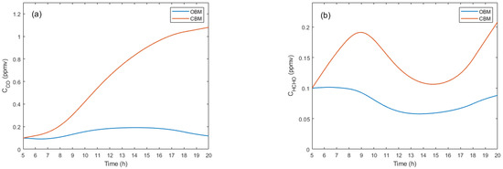
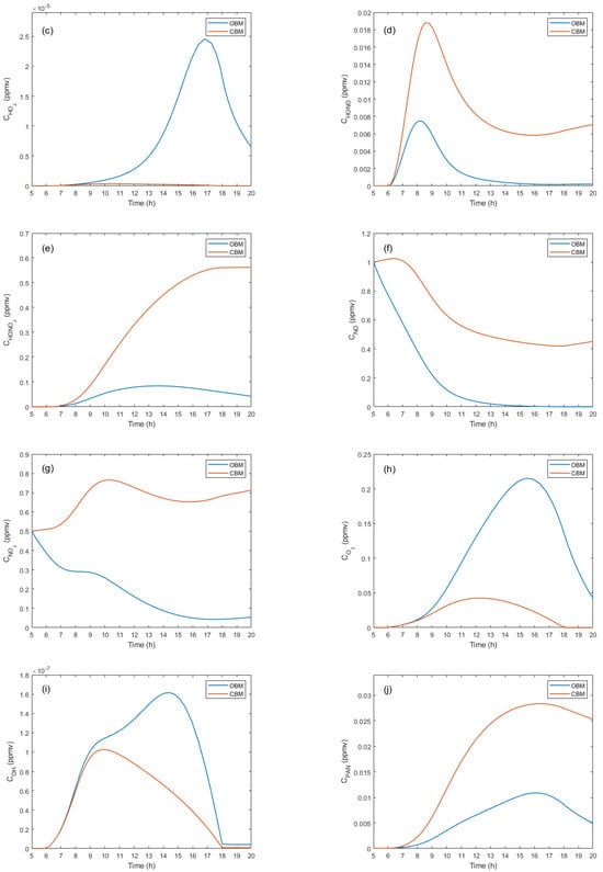
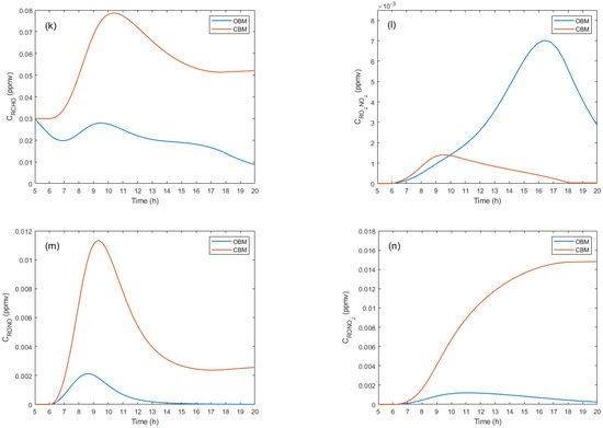
Figure 3.
Concentration profiles of the main pollutants.
In the CBM, higher concentrations of primary and secondary pollutants are observed compared to the OBM. However, in some cases, concentrations are lower in the CBM, which can be attributed to the complex system dynamics and the various physical, chemical, and photochemical factors involved.
Figure 3 shows the concentrations of the main pollutants, from which it can be observed that for carbon monoxide (see Figure 3a), the concentration is significantly higher in the CBM than in the OBM. In the CBM, the increase in occurs both in the absence and presence of solar radiation, with the latter increase being much more pronounced. In the OBM, the increase in concentration is more moderate and decreases further in the afternoon hours due to the absence of solar radiation. For formaldehyde (see Figure 3b), it is found that in both models, it is generated even in the absence of solar radiation; however, its concentration is higher in the CBM. With solar radiation, concentration variations increase considerably in both cases.
On the other hand, the concentration of nitric acid (), as shown in Figure 3e, is lower for the OBM due to the effect of the inflow, which facilitates the dispersion of the pollutant. The generation of depends on solar radiation, and its concentration stops increasing after 18:00 hours. Both models for nitrogen monoxide () show that the concentration tends to decrease (see Figure 3f), but it is always higher in the CBM. This compound is closely related to ozone generation. For nitrogen dioxide (), the CBM maintains higher concentrations (see Figure 3g), while in the OBM, the concentrations decrease due to the inflow of air.
In Figure 3h, the ozone () curve for the OBM shows lower concentrations with a behavior dependent on solar radiation. After 18:00 hours, no significant changes in concentrations are observed. However, for the OBM, a concentration peak is detected between 14:00 and 16:00 hours, attributable to the system dynamics. For the hydroxyl radical () profile, the CBM records higher concentrations due to the conditions and dynamics of the process (see Figure 3i). In both models, a direct dependence on solar radiation is observed before 6:00 hours and after 18:00 hours. The concentration is observed to be higher in the CBM (see Figure 3j), with its formation beginning with solar radiation at 6:00 hours. In the afternoon, its concentration decreases even in the absence of solar radiation due to ongoing chemical reactions. This behavior is also observed in the OBM, although at lower levels.
The concentration of higher aldehydes for the CBM reaches a peak around 10:00 hours and subsequently decreases due to interactions with other chemical species. In the OBM, the trend is similar but with lower levels due to advective transport, as shown in Figure 3k. For peroxyacyl nitrate, in the OBM, concentrations are higher and depend on solar radiation, especially in the morning hours (see Figure 3l). In the CBM, concentrations are lower but also dependent on solar radiation before 6:00 hours and after 18:00 hours.
Finally, the concentrations of alkyl nitrite are higher in the CBM, although both models show similar behavior (see Figure 3m). The generation of this compound depends on solar radiation, with a peak around 9:00 hours. After 15:00 hours, no significant changes are observed in either model. The concentration behavior of alkyl nitrate shows a constant increase for the CBM, which stops after 18:00 hours due to the absence of solar radiation. In the OBM, concentrations are lower due to the effect of advective transport. Both models depend on the onset of solar radiation for the formation of the compound.
4. Discussion
Kafle et al. and Tesche et al. use mathematical approaches to simulate pollutant dispersion using a modular model that integrates meteorology and chemical processes [24,27], whereas this study employs two models, CBM and OBM, with the latter being more detailed by considering factors such as altitude and airflow. The OBM model shows faster dispersion of pollutants due to the atmospheric dynamics included, compared to the CBM model. Additionally, peaks in photochemical pollutant concentrations (, , , etc.) are observed during hours of maximum solar radiation. This study reports a shift in these peaks toward the afternoon due to convective flow, which is more pronounced in the OBM model, as it incorporates more detail in air dynamics [32]. This behavior is similar to observations in studies on solar radiation dynamics in the atmosphere.
The influence of temperature on pollutant concentrations follows a similar trend in the CBM and OBM models. Some compounds show a direct relationship with temperature, while others show an inverse relationship. However, the concentrations obtained in the OBM model tend to be lower due to more efficient dispersion [36,40]. The relationship between temperature and pollutant concentration has also been explored in previous studies, where concentration peaks tend to rise with temperature for certain compounds [74].
The OBM model presents faster dispersion and lower concentrations compared to the CBM model, highlighting the importance of considering dynamic factors such as altitude and airflow in air quality simulations [43]. This is consistent with other studies showing that convective dispersion plays a key role in pollutant dispersion [38].
5. Conclusions
The study of gaseous pollution modeling in the troposphere reveals that the interaction of primary pollutants, such as nitrogen oxides and volatile organic compounds, under high solar radiation conditions, leads to the formation of tropospheric ozone and other secondary pollutants. Through the mathematical model, which includes 31 ordinary differential equations, it was demonstrated that the concentrations of most secondary pollutants peak at midday, indicating a direct correlation between solar radiation and the formation of photochemical smog. Additionally, a complex dynamic of pollutants is observed, with nonlinear concentration behaviors influenced by temperature factors and emission rates. Moreover, the study highlights the importance in considering both chemical mechanisms and environmental conditions for assessing air quality and its impact on public health and the environment. The implementation of “open-box” and “closed-box” models provides highly valuable tools for predicting pollution episodes and developing effective mitigation strategies.
Author Contributions
Conceptualization, L.A.C.-V. and J.T.M.-C., methodology, L.G.C.-P. and C.A.A.-D., software, D.G.M.-H. and H.R.C.-T., validation, C.G.-C. and O.J.R.-T., formal analysis, A.P.-N. and L.G.C.-P., investigation, J.T.M.-C. and A.P.-N., resources, H.R.C.-T. and O.J.R.-T., data curation, C.A.A.-D. and J.V.G.-F., writing—original draft preparation, J.V.G.-F. and L.A.C.-V., writing—review and editing, O.J.R.-T. and C.G.-C., visualization, J.V.G.-F. and L.A.C.-V., supervision, L.G.C.-P. and D.G.M.-H., project administration, D.G.M.-H. All authors have read and agreed to the published version of the manuscript.
Funding
This work was partially financed by Universidad Nacional del Callao.
Data Availability Statement
Data are contained within the article.
Conflicts of Interest
The authors declare no conflicts of interest.
References
- Ilić, P.; Popović, Z.; Nešković Markić, D. Assessment of Meteorological Effects and Ozone Variation in Urban Area. Ecol. Chem. Eng. 2020, 27, 373–385. [Google Scholar] [CrossRef]
- Manisalidis, I.; Stavropoulou, E.; Stavropoulos, A.; Bezirtzoglou, E. Environmental and Health Impacts of Air Pollution: A Review. Front. Public Health 2020, 8, 505570. [Google Scholar] [CrossRef]
- Wang, M.; Wang, J.; Wang, P.; Wang, Z.; Tang, S.; Qian, G.; Liu, T.; Chen, W. Multi-Pass Cavity-Enhanced Raman Spectroscopy of Complex Natural Gas Components. Anal. Chim. Acta 2025, 1336, 343463. [Google Scholar] [CrossRef]
- Chen, L.; Cui, B.; Zhang, C.; Hu, X.; Wang, Y.; Li, G.; Chang, L.; Liu, L. Impacts of Fuel Stage Ratio on the Morphological and Nanostructural Characteristics of Soot Emissions from a Twin Annular Premixing Swirler Combustor. Environ. Sci. Technol. 2024, 58, 10558–10566. [Google Scholar] [CrossRef]
- Chen, L.; Cao, Y.; Hu, X.; Zhang, B.; Chen, X.; Cui, B.; Xu, J.; Yu, T.; Xu, Z. Raman Spectral Optimization for Soot Particles: A Comparative Analysis of Fitting Models and Machine Learning Enhanced Characterization in Combustion Systems. Build Environ. 2025, 271, 112600. [Google Scholar] [CrossRef]
- Tao, L.; Wu, H.; Wang, J.; Li, B.; Wang, X.-Q.; Ning, P. Removal of SO2 from Flue Gas Using Bayer Red Mud: Influence Factors and Mechanism. J. Cent. South Univ. 2019, 26, 467–478. [Google Scholar] [CrossRef]
- Liu, Y.; Li, B.; Lei, X.; Liu, S.; Zhu, H.; Ding, E.; Ning, P. Novel Method for High-Performance Simultaneous Removal of NOx and SO2 by Coupling Yellow Phosphorus Emulsion with Red Mud. Chem. Eng. J. 2022, 428, 131991. [Google Scholar] [CrossRef]
- Paraschiv, S.; Barbuta-Misu, N.; Paraschiv, S.L. Influence of NO2, NO and Meteorological Conditions on the Tropospheric O3 Concentration at an Industrial Station. Energy Rep. 2020, 6, 231–236. [Google Scholar] [CrossRef]
- Rathore, A.; Gopikrishnan, G.S.; Kuttippurath, J. Changes in Tropospheric Ozone over India: Variability, Long-Term Trends and Climate Forcing. Atmos. Environ. 2023, 309, 119959. [Google Scholar] [CrossRef]
- Hoffman, F.M.; Nair, U.S.; Vanessa Adams, S.; Kai Juarez, E.; Petersen, M.R. A Comparison of Machine Learning Methods to Forecast Tropospheric Ozone Levels in Delhi. Atmosphere 2021, 13, 46. [Google Scholar] [CrossRef]
- Sahu, S.K.; Chen, L.; Liu, S.; Xing, J.; Mathur, R. Effect of Future Climate Change on Stratosphere-to-Troposphere-Exchange Driven Ozone in the Northern Hemisphere. Aerosol Air Qual. Res. 2023, 23, 220414. [Google Scholar] [CrossRef]
- Liu, P.; Song, H.; Wang, T.; Wang, F.; Li, X.; Miao, C.; Zhao, H. Effects of Meteorological Conditions and Anthropogenic Precursors on Ground-Level Ozone Concentrations in Chinese Cities. Environ. Pollut. 2020, 262, 114366. [Google Scholar] [CrossRef]
- Frei, M.; Ashrafuzzaman, M.; Piepho, H.P.; Herzog, E.; Begum, S.N.; Islam, M.M. Evidence for Tropospheric Ozone Effects on Rice Production in Bangladesh. Sci. Total Environ. 2024, 909, 168560. [Google Scholar] [CrossRef] [PubMed]
- Naqvi, H.R.; Mutreja, G.; Hashim, M.; Singh, A.; Nawazuzzoha, M.; Naqvi, D.F.; Siddiqui, M.A.; Shakeel, A.; Chaudhary, A.A.; Naqvi, A.R. Global Assessment of Tropospheric and Ground Air Pollutants and Its Correlation with COVID-19. Atmos. Pollut. Res. 2021, 12, 101172. [Google Scholar] [CrossRef] [PubMed]
- Madronich, S.; Sulzberger, B.; Longstreth, J.D.; Schikowski, T.; Andersen, M.P.S.; Solomon, K.R.; Wilson, S.R. Changes in Tropospheric Air Quality Related to the Protection of Stratospheric Ozone in a Changing Climate. Photochem. Photobiol. Sci. 2023, 22, 1129–1176. [Google Scholar] [CrossRef]
- Iungman, T.; Khomenko, S.; Barboza, E.P.; Cirach, M.; Gonçalves, K.; Petrone, P.; Erbertseder, T.; Taubenböck, H.; Chakraborty, T.; Nieuwenhuijsen, M. The Impact of Urban Configuration Types on Urban Heat Islands, Air Pollution, CO2 Emissions, and Mortality in Europe: A Data Science Approach. Lancet Planet. Health 2024, 8, e489–e505. [Google Scholar] [CrossRef]
- Chiacchiaretta, P.; Aruffo, E.; Mascitelli, A.; Colangeli, C.; Palermi, S.; Bianco, S.; Di Carlo, P. Inland O3 Production Due to Nitrogen Dioxide Transport Downwind a Coastal Urban Area: A Neural Network Assessment. Sustainability 2024, 16, 6355. [Google Scholar] [CrossRef]
- Wang, J.; Yang, Y.; Zhang, Y.; Niu, T.; Jiang, X.; Wang, Y.; Che, H. Influence of Meteorological Conditions on Explosive Increase in O3 Concentration in Troposphere. Sci. Total Environ. 2019, 652, 1228–1241. [Google Scholar] [CrossRef]
- Nguyen, D.H.; Lin, C.; Vu, C.T.; Cheruiyot, N.K.; Nguyen, M.K.; Le, T.H.; Lukkhasorn, W.; Vo, T.D.H.; Bui, X.T. Tropospheric Ozone and NOx: A Review of Worldwide Variation and Meteorological Influences. Environ. Technol. Innov. 2022, 28, 102809. [Google Scholar] [CrossRef]
- Real, E.; Megaritis, A.; Colette, A.; Valastro, G.; Messina, P. Atlas of Ozone Chemical Regimes in Europe. Atmos. Environ. 2024, 320, 120323. [Google Scholar] [CrossRef]
- Velázquez de Castro, F. Modelización y Análisis de Las Concentraciones de Ozono Troposférico; Universidad Complutense de Madrid, Servicio de Publicaciones: Ayreusburg, Spain, 2003; ISBN 978-84-669-1664-6. [Google Scholar]
- Jion, M.M.M.F.; Jannat, J.N.; Mia, M.Y.; Ali, M.A.; Islam, M.S.; Ibrahim, S.M.; Pal, S.C.; Islam, A.; Sarker, A.; Malafaia, G.; et al. A Critical Review and Prospect of NO2 and SO2 Pollution over Asia: Hotspots, Trends, and Sources. Sci. Total Environ. 2023, 876, 162851. [Google Scholar] [CrossRef] [PubMed]
- Malytska, L.; Ladstätter-Weißenmayer, A.; Galytska, E.; Burrows, J.P. Assessment of Environmental Consequences of Hostilities: Tropospheric NO2 Vertical Column Amounts in the Atmosphere over Ukraine in 2019–2022. Atmos. Environ. 2024, 318, 120281. [Google Scholar] [CrossRef]
- Kafle, J.; Adhikari, K.P.; Poudel, E.P.; Pant, R.R. Mathematical Modeling of Pollutants Dispersion in the Atmosphere. J. Nepal. Math. Soc. 2024, 7, 61–70. [Google Scholar] [CrossRef]
- McRae, G.J.; Goodin, W.R.; Seinfeld, J.H. Mathematical Modeling of Photochemical Air Pollution; Pasadena, CA, USA, 1982; Available online: https://core.ac.uk/download/pdf/216149675.pdf (accessed on 13 September 1999).
- Silva-Quiroz, R.; Rivera, A.L.; Ordoñez, P.; Gay-Garcia, C.; Frank, A. Atmospheric Blockages as Trigger of Environmental Contingencies in Mexico City. Heliyon 2019, 5, e02099. [Google Scholar] [CrossRef]
- Tesche, T.W. Comparison of Two Numerical Schemes for Integrating the Atmospheric Diffusion Equation: Evaluation with Atmospheric Data. Math. Model. 1987, 9, 507–519. [Google Scholar] [CrossRef]
- Lin, C.; Wang, Y.; Ooka, R.; Flageul, C.; Kim, Y.; Kikumoto, H.; Wang, Z.; Sartelet, K. Modeling of Street-Scale Pollutant Dis-persion by Coupled Simulation of Chemical Reaction, Aerosol Dynamics, and CFD. Atmos. Chem. Phys. 2023, 23, 1421–1436. [Google Scholar] [CrossRef]
- Leelőssy, Á.; Molnár, F.; Izsák, F.; Havasi, Á.; Lagzi, I.; Mészáros, R. Dispersion Modeling of Air Pollutants in the Atmosphere: A Review. Cent. Eur. J. Geosci. 2014, 6, 257–278. [Google Scholar] [CrossRef]
- Pisso, I.; Real, E.; Law, K.S.; Legras, B.; Bousserez, N.; Attié, J.L.; Schlager, H. Estimation of Mixing in the Troposphere from Lagrangian Trace Gas Reconstructions during Long-Range Pollution Plume Transport. J. Geophys. Res. Atmos. 2009, 114, 19301. [Google Scholar] [CrossRef]
- Ulfah, S.; Awalluddin, S. A; Wahidin. Advection-Diffusion Model for the Simulation of Air Pollution Distribution from a Point Source Emission. J. Phys. Conf. Ser. 2018, 948, 012067. [Google Scholar] [CrossRef]
- Moreira, D.; Xavier, P.; Palmeira, A.; Nascimento, E. New Approach to Solving the Atmospheric Pollutant Dispersion Equation Using Fractional Derivatives. Int. J. Heat. Mass. Transf. 2019, 144, 118667. [Google Scholar] [CrossRef]
- Ravshanov, N.; Muradov, F.; Akhmedov, D. Operator Splitting Method for Numerical Solving the Atmospheric Pollutant Dispersion Problem. J. Phys. Conf. Ser. 2020, 1441, 012164. [Google Scholar] [CrossRef]
- Atkinson, R.; Lloyd, A.C. Evaluation of Kinetic and Mechanistic Data for Modeling of Photochemical Smog. J. Phys. Chem. Ref. Data 1984, 13, 315–444. [Google Scholar] [CrossRef]
- Atkinson, R.; Baulch, D.L.; Cox, B.A.; Hampson, R.F.; Kerr, J.A.; Troe, J. Towards a Quantitative Understanding of Atmospheric Ozone. Planet. Space Sci. 1989, 37, 1605–1620. [Google Scholar] [CrossRef]
- Brewer, D.A.; Augustsson, T.R.; Levine, J.S. The Photochemistry of Anthropogenic Nonmethane Hydrocarbons in the Tropo-sphere. J. Geophys. Res. 1983, 88, 6683–6695. [Google Scholar] [CrossRef]
- Rawat, P.; Naja, M.; Rajwar, M.C.; Irie, H.; Lerot, C.; Kumar, M.; Lal, S. Long-Term Observations of NO2, SO2, HCHO, and CHOCHO over the Himalayan Foothills: Insights from MAX-DOAS, TROPOMI, and GOME-2. Atmos. Environ. 2024, 336, 120746. [Google Scholar] [CrossRef]
- Gao, T.; Xu, D.; Mi, Y.; Lu, Y. Simulation Analysis of NO2 Pollution Diffusion Law Based on Gauss Plume Model: A Case Study from Hebei Province. IOP Conf. Ser. Earth Environ. Sci. 2020, 555, 012090. [Google Scholar] [CrossRef]
- Narasimhan, R.; Keller, J.; Subramaniam, G.; Raasch, E.; Croley, B.; Duncan, K.; Potter, W.T. Ozone Modeling Using Neural Networks. J. Appl. Meteorol. 2000, 39, 291–296. [Google Scholar] [CrossRef]
- Seinfeld, J.H.; Pandis, S.N. Atmospheric Chemistry and Physics: From Air Pollution to Climate Change, 3rd ed.; John Wiley & Sons: Hoboken, NJ, USA, 2019; ISBN 978-1-118-94740-1. [Google Scholar]
- Atkinson, R.; Baulch, D.L.; Cox, R.A.; Crowley, J.N.; Hampson, R.F.; Hynes, R.G.; Jenkin, M.E.; Rossi, M.J.; Troe, J.; Wallington, T.J. Evaluated Kinetic and Photochemical Data for Atmospheric Chemistry: Volume IV–Gas Phase Reactions of Organic Halogen Species. Atmos. Chem. Phys. 2008, 8, 4141–4496. [Google Scholar] [CrossRef]
- Calvert, J.G. The Chemistry of the Atmosphere: Its Impact on Global Change, 1st ed.; Blackwell Publishing: Oxford, UK, 1994. [Google Scholar]
- Grell, G.A.; Peckham, S.E.; Schmitz, R.; McKeen, S.A.; Frost, G.; Skamarock, W.C.; Eder, B. Fully Coupled “Online” Chemistry within the WRF Model. Atmos. Environ. 2005, 39, 6957–6975. [Google Scholar] [CrossRef]
- Simpson, D.; Benedictow, A.; Berge, H.; Bergström, R.; Emberson, L.D.; Fagerli, H.; Flechard, C.R.; Hayman, G.D.; Gauss, M.; Jonson, J.E.; et al. The EMEP MSC-W Chemical Transport Model – Technical Description. Atmos. Chem. Phys. 2012, 12, 7825–7865. [Google Scholar] [CrossRef]
- Lu, X.; Zhang, L.; Wu, T.; Long, M.S.; Wang, J.; Jacob, D.J.; Zhang, F.; Zhang, J.; Eastham, S.D.; Hu, L.; et al. Development of the Global Atmospheric Chemistry General Circulation Model BCC-GEOS-Chem v1.0: Model Description and Evaluation. Geosci. Model. Dev. 2020, 13, 3817–3838. [Google Scholar] [CrossRef]
- Emery, C.; Baker, K.; Wilson, G.; Yarwood, G. Comprehensive Air Quality Model with Extensions: Formulation and Evaluation for Ozone and Particulate Matter over the US. Atmosphere 2024, 15, 1158. [Google Scholar] [CrossRef]
- Falls, A.H.; McRae, G.J.; Seinfeld, J.H. Sensitivity and Uncertainty of Reaction Mechanisms for Photochemical Air Pollution. Int. J. Chem. Kinet. 1979, 11, 1137–1162. [Google Scholar] [CrossRef]
- Bazzell, C.C.; Peters, L.K. The Transport of Photochemical Pollutants to the Background Troposphere. Atmos. Environ. (1967) 1981, 15, 957–968. [Google Scholar] [CrossRef]
- Krysztofiak, G.; Catoire, V.; Poulet, G.; Marécal, V.; Pirre, M.; Louis, F.; Canneaux, S.; Josse, B. Detailed Modeling of the At-mospheric Degradation Mechanism of Very-Short Lived Brominated Species. Atmos. Environ. 2012, 59, 514–532. [Google Scholar] [CrossRef]
- Hampson, R.F.; Garvin, D. Reaction Rate and Photochemical Data for Atmospheric Chemistry, 1977; US Department of Commerce, National Bureau of Standards: Gaithersburg, MD, USA, 1978; Volume 513.
- Leone, J.A.; Seinfeld, J.H. Comparative Analysis of Chemical Reaction Mechanisms for Photochemical Smog. Atmos. Environ. (1967) 1985, 19, 437–464. [Google Scholar] [CrossRef]
- Kyan, C.P.; Seinfeld, J.H. Determination of Optimal Multiyear Air Pollution Control Policies. J. Dyn. Syst. Meas. Control 1972, 94, 266–274. [Google Scholar] [CrossRef]
- McRae, G.J.; Goodin, W.R.; Seinfeld, J.H. Mathematical Modelling of Photochemical Air Pollution. In Proceedings of the AIAA Monographs, Pasadena, CA, USA, 18 June 1982; Volume 25, pp. 67–77. [Google Scholar]
- McRae, G.J.; Goodin, W.R.; Seinfeld, J.H. Numerical Solution of the Atmospheric Diffusion Equation for Chemically Reacting Flows. J. Comput. Phys. 1982, 45, 1–42. [Google Scholar] [CrossRef]
- Cutlip, M.B.; Shacham, M. Resolucion de Problemas En Ingenieria Quimica y Bioquimica Con POLYMATH, EXCEL y MATLAB, 2nd ed.; Prentice Hall: Madrid, Spain, 2008; ISBN 9788483224618. [Google Scholar]
- Ahrens, C.D.; Henson, R. Meteorology Today: An Introduction to Weather, Climate, and the Environment, 12th ed.; Brooks Cole: Boston, MA, USA, 2018. [Google Scholar]
- Burden, R.L.; Faires, J.D. Numerical Analysis, 9th ed.; Brooks/Cole, Cencag Learning: Boston, MA, USA, 2011. [Google Scholar]
- Hairer, E.; Wanner, G. Solving Ordinary Differential Equations II; Springer Series in Computational Mathematics; Springer: Berlin/Heidelberg, Germany, 1996; Volume 14, ISBN 978-3-642-05220-0. [Google Scholar]
- Erickson, L.E.; Newmark, G.L.; Higgins, M.J.; Wang, Z. Nitrogen Oxides and Ozone in Urban Air: A Review of 50 plus Years of Progress. Env. Prog. Sustain. Energy 2020, 39, e13484. [Google Scholar] [CrossRef]
- Monks, P.S.; Archibald, A.T.; Colette, A.; Cooper, O.; Coyle, M.; Derwent, R.; Fowler, D.; Granier, C.; Law, K.S.; Mills, G.E.; et al. Tropospheric Ozone and Its Precursors from the Urban to the Global Scale from Air Quality to Short-Lived Climate Forcer. Atmos. Chem. Phys. 2015, 15, 8889–8973. [Google Scholar] [CrossRef]
- Finlayson-Pitts, B.J.; Pitts, J.N. Chemistry of the Upper and Lower Atmosphere: Theory, Experiments, and Applications; Academic Press: San Diego, CA, USA, 1999. [Google Scholar]
- Xuan, H.; Zhao, Y.; Ma, Q.; Chen, T.; Liu, J.; Wang, Y.; Liu, C.; Wang, Y.; Liu, Y.; Mu, Y.; et al. Formation mechanisms and atmospheric implications of summertime nitrous acid (HONO) during clean, ozone pollution and double high-level PM2.5 and O3 pollution periods in Beijing. Sci. Total Environ. 2023, 857, 159538. [Google Scholar] [CrossRef] [PubMed]
- Elshorbany, Y.; Ziemke, J.R.; Strode, S.; Petetin, H.; Miyazaki, K.; De Smedt, I.; Pickering, K.; Seguel, R.J.; Worden, H.; Emmerichs, T.; et al. Tropospheric Ozone Precursors: Global and Regional Distributions, Trends, and Variability. Atmos. Chem. Phys. 2024, 24, 12225–12257. [Google Scholar] [CrossRef]
- Lodge, J.P. Determination of C1–C5 Aldehydes in Ambient Air and Source Emissions as 2,4-Dinitrophenylhydrazones by HPLC. In Methods of Air Sampling and Analysis; Routledge: New York, NY, USA, 2017; pp. 293–295. [Google Scholar]
- Gilman, J.B.; Lerner, B.M.; Kuster, W.C.; Goldan, P.D.; Warneke, C.; Veres, P.R.; Roberts, J.M.; De Gouw, J.A.; Burling, I.R.; Yokelson, R.J. Biomass Burning Emissions and Potential Air Quality Impacts of Volatile Organic Compounds and Other Trace Gases from Fuels Common in the US. Atmos. Chem. Phys. 2015, 15, 13915–13938. [Google Scholar] [CrossRef]
- Jacob, D.J. Introduction to Atmospheric Chemistry; Princeton University Press: Princeton, NJ, USA, 1999. [Google Scholar]
- Atkinson, R. Atmospheric Chemistry of VOCs and NOx. Atmos. Environ. 2000, 34, 2063–2101. [Google Scholar] [CrossRef]
- Travis, K.R.; Nault, B.A.; Crawford, J.H.; Bates, K.H.; Blake, D.R.; Cohen, R.C.; Fried, A.; Hall, S.R.; Huey, L.G.; Lee, Y.R.; et al. Impact of Improved Representation of Volatile Organic Compound Emissions and Production of NOx Reservoirs on Modeled Urban Ozone Production. Atmos. Chem. Phys. 2024, 24, 9555–9572. [Google Scholar] [CrossRef]
- Carter, W.P.L. Documentation of the SAPRC-99 Chemical Mechanism for VOC Reactivity Assessment; Riverside; Air Pollution Research Center and College of Engineering: Carmel, CA, USA, 1999; Available online: https://intra.engr.ucr.edu/~carter/pubs/s99doc.pdf (accessed on 13 September 1999).
- Jacob, D.J.; Wofsy, S.C. Photochemistry of Biogenic Emissions over the Amazon Forest. J. Geophys. Res. 1988, 93, 1477–1486. [Google Scholar] [CrossRef]
- Sun, Y.; Wang, L.; Wang, Y.; Quan, L.; Zirui, L. In Situ Measurements of SO2, NOx, NOy, and O3 in Beijing, China during August 2008. Sci. Total Environ. 2011, 409, 933–940. [Google Scholar] [CrossRef]
- Atkinson, R. Gas-Phase Tropospheric Chemistry of Organic Compounds: A Review. Atmos. Environ. Part A Gen. Top. 1990, 24, 1–41. [Google Scholar] [CrossRef]
- Goldstein, A.H.; Galbally, I.E. Known and Unexplored Organic Constituents in the Earth’s Atmosphere. Environ. Sci. Technol. 2007, 41, 1514–1521. [Google Scholar] [CrossRef]
- Jung, J.; Choi, Y.; Souri, A.H.; Mousavinezhad, S.; Sayeed, A.; Lee, K. The Impact of Springtime-Transported Air Pollutants on Local Air Quality With Satellite-Constrained NOx Emission Adjustments Over East Asia. J. Geophys. Res. Atmos. 2022, 127, e2021JD035251. [Google Scholar] [CrossRef]
Disclaimer/Publisher’s Note: The statements, opinions and data contained in all publications are solely those of the individual author(s) and contributor(s) and not of MDPI and/or the editor(s). MDPI and/or the editor(s) disclaim responsibility for any injury to people or property resulting from any ideas, methods, instructions or products referred to in the content. |
© 2025 by the authors. Licensee MDPI, Basel, Switzerland. This article is an open access article distributed under the terms and conditions of the Creative Commons Attribution (CC BY) license (https://creativecommons.org/licenses/by/4.0/).