An Enhanced Logic-Based Bender’s Decomposition Algorithm with Proximity Principle for Simulator-Based Distillation Process Optimization

Abstract

The optimization of distillation processes is particularly challenging due to the presence of nonlinear equations and integer variables, resulting in complex mixed-integer nonlinear programming (MINLP) problems. This work introduces an enhanced optimization algorithm, the logic-based proximity principle Bender’s decomposition (LB-PBD), to address non-convex MINLP issues in simulator-based distillation optimization. The key innovation, the proximity principle, improves lower bound predictions by prioritizing information from the closest known integer solutions. Additionally, the integration of a multi-start points strategy and a delayed convergence strategy ensures the algorithm achieves global optimality while avoiding premature convergence. The effectiveness if the proposed LB-PBD is validated through three case studies. Numerical experiments demonstrate so-called proximity principle superior ability of original algorithm to navigate local optima, making LB-PBD more versatile than traditional deterministic algorithm (logic-based outer approximation algorithm) and stochastic algorithm (adaptive superstructure-differential evolution algorithm). In a single-column distillation case, LB-PBD achieves high accuracy. In an extractive distillation case, the algorithm successfully optimizes the separation of a near-azeotropic mixture, reducing energy consumption and improving product recovery compared to previous solutions. These results highlight LB-PBD as a robust and effective tool for solving non-convex MINLLP problems, particularly in simulator-based distillation process optimization.

1. Introduction

Distillation is one of the most widely used industrial separation methods, often preferred by engineers due to its established process and simplicity. It is estimated that distillation accounts for 90–95% [1] of liquid separations in industry. However, the high energy consumption associated with distillation has been a long-standing criticism. It is estimated that distillation operations contribute to 10–15% [2] of global energy consumption. To mitigate this, engineers strive to minimize energy consumption during the early stages of design. However, typical distillation processes involve numerous integer variables and nonlinear equations, which make optimization a challenging mixed-integer nonlinear programming (MINLP) problem.

Most distillation designs rely on process simulators, such as Aspen and ProII. These simulators commonly employ the sequential modular (SM) method as their default solving algorithm due to its stability. However, SM algorithms cannot provide direct derivative information for continuous variables, leading to the treatment of the problem as a derivative-free optimization (DFO) [3]. DFO methods iteratively generate new prediction points based on known samples of independent and dependent variables. Classic DFO approaches include differential evolution [4,5], particle swarm optimization [6,7], and genetic algorithms (GA) [8,9], along with various improved versions [10]. DFO is particularly powerful in multi-objective optimization, as it can identify Pareto frontiers [11].

However, DFO methods face challenges, such as the lack of a stationary point criterion, like the Karush–Kuhn–Tucker (KKT) conditions. Additionally, the setting of termination conditions and hyperparameters is highly related to the problem, and it is difficult to ensure the accuracy and speed of solving unknown problems using specific parameters.

An alternative approach involves using equation-oriented (EO) [12,13] or perturbation methods [14] to derive continuous variable derivatives and mathematical programming for integer variables, constituting deterministic algorithms. Famous deterministic algorithms include branch and bound [15], generalized Bender’s decomposition (GBD) [16], outer approximation (OA) [17], and extended cutting plane algorithms (ECP) [18]. Nevertheless, many deterministic algorithms were initially designed for convex programming, which poses challenges in avoiding local optima.

Many solutions have been proposed by researchers to avoid the algorithm’s solution being limited to local optima. In nonlinear programming (NLP), the multi-start strategy [19] is highly effective. Increasing the number of starting points enhances the likelihood of finding global optima. Similarly, a hot start method [20] was proposed, which solves multiple NLP subproblems before iterations, while Su et al. [21] extended this by incorporating hot starts into each iteration, allowing parallel computation without significantly increasing optimization time. The n-step restart strategy or segmented strategy, frequently used in NLP, can also improve the deterministic algorithms in MINLP. Franke [22] modified the GBD strategy by discarding Lagrangian functions after convergence and re-establishing MILP from the optimal integer solution. Similarly, Javaloyes-Antón et al. [23] improved ECP by intermittently relaxing and modifying constraints. Bergamini et al. [24] employed the McCormick envelope for piecewise linearization, enhancing the probability of global optima and adopted by solvers like Gurobi [25]. These techniques can be extended to other deterministic algorithms.

In order to reduce the dependence of deterministic algorithm solutions on the initial point, Chia et al. [26] provided starting points for OA using GA, while Liñán et al. [27] proposed hybrid algorithms that combine stochastic (Differential Evolution with Tabu List) and deterministic methods (discrete-steepest descent algorithm with variable bounding). These hybrid algorithms narrow the search domain of deterministic methods, improving global optima discovery. However, a fundamental issue still exists: It is impossible to determine in advance that the programming within the narrowed search space is convex, which means that the solution quality of hybrid algorithms is still dependent on deterministic algorithms because the final solution is obtained by a deterministic algorithm to ensure that it meets the mathematical criteria for determining the optimal solution.

When examining existing convex deterministic algorithms, a key limitation of most in non-convex programming is their reliance on gradient information (or difference information for integer variables) from all known points to construct constraint conditions and derive the lower bound of the original problem. In convex functions, as shown in Figure 1a, this lower bound prediction (represented by the red line) is accurate. However, for non-convex functions, as shown in Figure 1b, this prediction no longer serves as a lower bound but instead becomes an “upper bound prediction”. This occurs because the executed programming behaves like a min–max programming, ultimately leading to premature convergence of the algorithm.

To address this limitation, if the lower bound of the unknown point is constrained solely by information from its nearest known point (illustrated by the blue line in Figure 1), the method maintains an accurate lower bound prediction for convex functions while improving lower bound accuracy for non-convex functions. This concept, so-called the proximity principle, will be discussed in detail in Section 2.

The first deterministic algorithm applied in simulator-based distillation optimization is the logic-based outer approximation algorithm (LB-OA), a variant of OA [14,28]. This method transforms the mixed-integer linear programming (MILP) problem into mixed binary linear programming (MBLP) using logical variables, allowing a single inequality to contain information from multiple integer combinations. Additionally, generalized disjunctive programming (GDP) [29], which addresses disjunctive terms in models, can be applied using big-M or hull reform. The use of penalty functions to incorporate constraints into the objective function [30] further improves algorithm robustness, making deterministic algorithms widely applicable in simulator-based optimization. In simulation-based distillation optimization, it is challenging to decouple integer variables from continuous ones, meaning that the MINLP to be solved does not conform to the assumptions of the LB-OA method, making it impossible to guarantee the global optimality of the final solution.

On the other hand, Liñán et al. [31] propose a Bender’s decomposition (BD) framework, which excludes continuous variables in the MILP master problem, is more appropriate for simulator-based distillation optimization. Compared to GBD, BD does not rely on Lagrange multipliers, which are difficult to provide reliably in NLP due to numerical issues. Thus, BD proves to be more suitable in this context.

The organization of this paper is as follows: Section 2 introduces the proximity principle and the proposed improved algorithms. Section 3 demonstrates the effectiveness of the improvements through a numerical case and two simulation-based optimization case studies. The conclusions are presented in Section 4.

2. Materials and Methods

2.1. Problem Statement and Logic-Based Bender’s Decomposition Algorithm

Process simulator-based distillation optimization problem can be formulated as a mixed-integer nonlinear programming (MINLP), represented as follows:

$$(\mathit{x},\mathit{y})=arg\min \left\{f_{MINLP}=F\left(\mathit{x},\mathit{y},\mathit{u}\right)\right\}$$

(1)

Subject to the following:

$$\mathit{U}(\mathit{x},\mathit{y},\mathit{u})=\mathbf{0}$$

(2)

$$\mathit{G}(\mathit{x},\mathit{y},\mathit{u})=\left[g_m\left(\mathit{x},\mathit{y},\mathit{u}\right)\right]=\left[\begin{array}{c}{g}_1\left(\mathit{x},\mathit{y},\mathit{u}\right)\\ ⋮\\ g_{\dim (\mathit{G})}\left(\mathit{x},\mathit{y},\mathit{u}\right)\end{array}\right]\le \mathbf{0}$$

(3)

$$\begin{gathered} {\mathit{x}}^{\mathit{l}\mathit{b}}\le \mathit{x}\le {\mathit{x}}^{\mathit{u}\mathit{b}},{\mathit{y}}^{\mathit{l}\mathit{b}}=\left[y_p^{lb}\right]\le \mathit{y}=\left[y_p\right]\le {\mathit{y}}^{\mathit{u}\mathit{b}}=\left[y_p^{ub}\right] \\ \mathit{x}\in {\mathbb{R}}^{\dim \left(\mathit{x}\right)},\mathit{y}\in {\mathbb{N}}^{\dim \left(\mathit{y}\right)},m\in {\mathcal{N}}_1,p\in {\mathcal{N}}_2 \\ {\mathcal{N}}_1=\left\{\mathrm{1,2},\dots ,\dim (\mathit{G})\right\} \\ {\mathcal{N}}_2=\{\mathrm{1,2},\dots ,\dim (\mathit{y})\} \end{gathered}$$

where the input variables of the simulator consist of $\mathit{x}$ and $\mathit{y}$. $\mathit{x}$ is a series of continuous variables, such as the reflux ratio of the distillation column, the temperature of the heat exchanger, etc. $\mathit{y}$ represents a series of integer variables $y_p$, such as the number of trays in the distillation column. $\mathit{u}$ is the output of the simulator, such as the heat duty of heat exchanger, top temperature of distillation column, etc. $F\left(\mathit{x},\mathit{y},\mathit{u}\right)$ is the objective function of the design, which can be an energy consumption target or a CO₂ emission target, and the most commonly used is the total annualized cost (TAC). $\mathit{U}(\mathit{x},\mathit{y},\mathit{u})$ represents a series of implicit equation systems that represent the calculation process of the simulator. As far as we know, the steady-state calculation process does not include inequality constraints. $\mathit{G}(\mathit{x},\mathit{y},\mathit{u})$ is a series of constraints functions $g_m\left(\mathit{x},\mathit{y},\mathit{u}\right)$, such as purity constraints, temperature constraints, flow constraints, etc. Note that equality constraints can be expressed through two inequality constraints.

The logic-based Bender’s decomposition algorithm (LB-BD) decomposes MINLP into nonlinear programming (NLP) subproblem, which is Formulas (4)–(6):

$$\mathit{x}=\arg \min \left\{f_{NLP}=f\left(\mathit{x},{\mathit{y}}^{\mathrm{*}},\mathit{u}\right)\right\}$$

(4)

Subject to the following:

$$\mathit{U}\left(\mathit{x},{\mathit{y}}^{\mathrm{*}},\mathit{u}\right)=\mathbf{0}$$

(5)

$$\mathit{G}\left(\mathit{x},{\mathit{y}}^{\mathrm{*}},\mathit{u}\right)\le \mathbf{0}$$

(6)

$${\mathit{x}}^{\mathit{l}\mathit{b}}\le \mathit{x}\le {\mathit{x}}^{\mathit{u}\mathit{b}},\mathit{x}\in {\mathbb{R}}^{\dim \left(\mathit{x}\right)}$$

And mixed-integer linear programming (MILP) master problem, which is Formulas (7)–(15):

$$\mathit{y}=\arg \min \left\{f_{MILP}=\alpha +M\sum _{m\in {\mathcal{N}}_2}{\beta }_m\right\}$$

(7)

Subject to the following:

$$K_n\left(\mathit{y},{\mathit{y}}_{\mathit{n}}^{\mathrm{*}},{\mathit{n}}_{\mathit{p}},B_{p,q},q\right)\le \alpha$$

(8)

$$W_{m,n}\left(\mathit{y},{\mathit{y}}_{\mathit{n}}^{\mathrm{*}},{\mathit{n}}_{\mathit{p}},B_{p,q},q\right)\le {\beta }_m$$

(9)

$$y_p=\sum _{q=1}^{y_p^{ub}-y_p^{lb}+1}\left(y_p^{lb}+q-1\right)B_{p,q}$$

(10)

$$\sum _{q=1}^{y_p^{ub}-y_p^{lb}+1}{B}_{p,q}=1$$

(11)

$$\sum _{p\in {\mathcal{N}}_3}{B}_{p,y_{p,n}^{\mathrm{*}}-y_p^{lb}+1}\le \dim \left(\overrightarrow{\mathit{y}}\right)-1$$

(12)

$$\begin{gathered} {\mathit{y}}^{\mathit{l}\mathit{b}}\le \mathit{y}\le {\mathit{y}}^{\mathit{u}\mathit{b}},\mathit{y}\in {\mathbb{N}}^{\dim \left(\mathit{y}\right)} \\ {\mathit{n}}_{\mathit{w}}=\left[\begin{array}{c}{n}_{1,w}\\ ⋮\\ n_{\dim \left(\overrightarrow{\mathit{y}}\right),w}\end{array}\right],n_{w,w}=1,n_{p,w}=0,p\ne w \\ \alpha ,{\beta }_m\in \mathbb{R},{\beta }_m\ge 0,B_{p,q}\in \left\{\mathrm{0,1}\right\},m\in {\mathcal{N}}_1,p,w\in {\mathcal{N}}_2,n\in {\mathcal{N}}_3 \\ {\mathcal{N}}_1=\left\{\mathrm{1,2},\dots ,\dim (\mathit{G})\right\} \\ {\mathcal{N}}_2=\{\mathrm{1,2},\dots ,\dim (\mathit{y})\} \\ {\mathcal{N}}_3=\{\mathrm{1,2},\dots ,\mathrm{N}\mathrm{u}\mathrm{m}\mathrm{b}\mathrm{e}\mathrm{r}\mathrm{o}\mathrm{f}\mathrm{k}\mathrm{n}\mathrm{o}\mathrm{w}\mathrm{n}\mathrm{p}\mathrm{o}\mathrm{i}\mathrm{n}\mathrm{t}\mathrm{s}{\mathit{y}}_{\mathit{n}}^{\mathrm{*}}\mathrm{i}\mathrm{n}\mathrm{M}\mathrm{I}\mathrm{L}\mathrm{P}\} \end{gathered}$$

where $\alpha$ is the relaxation variable for the objective function $f$, and ${\beta }_m$ is the relaxation variable for the m-th constraint function $g_m$. For every set of ${\mathit{y}}_{\mathit{n}}^{\mathit{*}}$, there will be a set of Formulas (8) and (9). $B_{p,q}$ is a 0–1 variable, when it is 1, it represents that the p-th integer variable is $(y_p^{lb}+q-1)$, otherwise it is not. $\left[B_{p,q}\right]$ corresponds one-to-one with $\mathit{y}$ through Formulas (10) and (11), whose quantity is equal to that of integer variables. And avoids situations $\mathit{y}={\mathit{y}}_{\mathit{n}}^{\mathit{*}}$ by Formula (12). ${\mathit{n}}_{\mathit{p}}$ is a unit vector. $M$ is a sufficiently large number to reject the infeasible solution.

$K_n\left(\mathit{y},{\mathit{y}}_{\mathit{n}}^{\mathit{*}},{\mathit{n}}_{\mathit{p}},B_{p,q},q\right)$ ($W_{m,n}\left(\mathit{y},{\mathit{y}}_{\mathit{n}}^{\mathit{*}},{\mathit{n}}_{\mathit{p}},B_{p,q},q\right)$) is the lower bound estimate of the objective function (constraint function) based on the known points $({\mathit{x}}_{\mathit{n}}^{\mathit{*}},{\mathit{y}}_{\mathit{n}}^{\mathit{*}})$ (solutions of NLP subproblem), using linear extrapolation, written as follows:

$$K_n\left(\mathit{y},{\mathit{y}}_{\mathit{n}}^{\mathrm{*}},{\mathit{n}}_{\mathit{p}},B_{p,q},q\right)=f_n\left({\mathit{y}}_{\mathit{n}}^{\mathrm{*}}\right)+{\displaystyle \sum _{p=1}^{\dim (\mathit{y})}}\left\{\begin{array}{c}{\displaystyle \sum _{q=1}^{y_p^{\mathrm{*}}-y_p^{lb}}}\left(f\left({\mathit{y}}_{\mathit{n}}^{\mathrm{*}}-{\mathit{n}}_{\mathit{p}}\right)-f_n\left({\mathit{y}}_{\mathit{n}}^{\mathrm{*}}\right)\right)\left(y_{p,n}^{\mathrm{*}}-\left(y_p^{lb}+q-1\right)\right)B_{p,q}\\ +{\displaystyle \sum _{q=y_p^{\mathrm{*}}-y_p^{lb}+2}^{y_p^{ub}-y_p^{lb}+1}}\left(f\left({\mathit{y}}_{\mathit{n}}^{\mathrm{*}}+{\mathit{n}}_{\mathit{p}}\right)-f_n\left({\mathit{y}}_{\mathit{n}}^{\mathrm{*}}\right)\right)\left(\left(y_p^{lb}+q-1\right)-y_{p,n}^{\mathrm{*}}\right)B_{p,q}\end{array}\right\}$$

(13)

$$W_{m,n}\left(\mathit{y},{\mathit{y}}_{\mathit{n}}^{\mathrm{*}},{\mathit{n}}_{\mathit{p}},B_{p,q},q\right)=g_{m,n}\left({\mathit{y}}_{\mathit{n}}^{\mathrm{*}}\right)+{\displaystyle \sum _{p=1}^{\dim (\mathit{y})}}\left\{\begin{array}{c}{\displaystyle \sum _{q=1}^{y_p^{\mathrm{*}}-y_p^{lb}}}\left(g_m\left({\mathit{y}}_{\mathit{n}}^{\mathrm{*}}-{\mathit{n}}_{\mathit{p}}\right)-g_{m,n}\left({\mathit{y}}_{\mathit{n}}^{\mathrm{*}}\right)\right)\left(y_{p,n}^{\mathrm{*}}-\left(y_p^{lb}+q-1\right)\right)B_{p,q}\\ +{\displaystyle \sum _{q=y_p^{\mathrm{*}}-y_p^{lb}+2}^{y_p^{ub}-y_p^{lb}+1}}\left(g_m\left({\mathit{y}}_{\mathit{n}}^{\mathrm{*}}+{\mathit{n}}_{\mathit{p}}\right)-g_{m,n}\left({\mathit{y}}_{\mathit{n}}^{\mathrm{*}}\right)\right)\left(\left(y_p^{lb}+q-1\right)-y_{p,n}^{\mathrm{*}}\right)B_{p,q}\end{array}\right\}$$

(14)

In the above formula, the summation formula satisfies the following constraints:

$$ifa>b,then\sum _{i=a}^{b}x=0,a,b\in \forall \mathbb{N}$$

(15)

where ${\mathit{y}}_{\mathit{n}}^{\mathit{*}}-{\mathit{n}}_{\mathit{p}}$ and ${\mathit{y}}_{\mathit{n}}^{\mathit{*}}+{\mathit{n}}_{\mathit{p}}$ is the neighborhood of the ${\mathit{y}}_{\mathit{n}}^{\mathit{*}}$. $f\left({\mathit{y}}_{\mathit{n}}^{\mathit{*}}-{\mathit{n}}_{\mathit{p}}\right)$, $g_m\left({\mathit{y}}_{\mathit{n}}^{\mathit{*}}-{\mathit{n}}_{\mathit{p}}\right)$ is the solution of NLP subproblem (Formulas (4)–(6)) with fixed integer combination ${\mathit{y}}_{\mathit{n}}^{\mathit{*}}-{\mathit{n}}_{\mathit{p}}$, and the same expression also applies to ${\mathit{y}}_{\mathit{n}}^{\mathit{*}}+{\mathit{n}}_{\mathit{p}}$ and ${\mathit{y}}_{\mathit{n}}^{\mathit{*}}$.

An example is presented to help readers understand Formula (13), assuming that the objective function $f\left(y\right)$ is a typical quadratic function, written as follows:

$$f\left(y\right)=y^2,-4\le y\le 4,y\in \mathbb{N}$$

(16)

The real function value is represented by the black solid dots in Figure 2, assuming that the known point ${\mathit{y}}_{\mathit{n}}^{\mathit{*}}=0$, as indicated by the red circle in Figure 2.

Due to the dimension of $y$ being 1, which means the upper limit of $p$ is 1, $y_1^{lb}=-4$, $y_1^{ub}=4$, and $n_p$ has only one vector: $n_1=1$. Then, there are $f\left({\mathit{y}}_{\mathit{n}}^{\mathit{*}}-{\mathit{n}}_{\mathit{p}}\right)=f\left(-1\right)=1$ and $f\left({\mathit{y}}_{\mathit{n}}^{\mathit{*}}+{\mathit{n}}_{\mathit{p}}\right)=f\left(1\right)=1$. There are 9 $B_{p,q}$, each corresponding to the value of $y$ one by one according to Formulas (10) and (11). For example, when $B_{\mathrm{1,3}}=1$, all other $B_{p,q}$ are 0, and $y=-2$. Due to the limitation of Formula (12), $B_{\mathrm{1,5}}=1$ cannot be the solution to the MILP. In summary, Formula (13) can be simplified as follows, as indicated by the red dashed line in Figure 2:

$$K_n\left(\mathit{y},{\mathit{y}}_{\mathit{n}}^{\mathrm{*}},{\mathit{n}}_{\mathit{p}},B_{p,q},q\right)=K_n\left(B_{p,q}\right)=4B_{\mathrm{1,1}}+3B_{\mathrm{1,2}}+2B_{\mathrm{1,3}}+B_{\mathrm{1,4}}+B_{\mathrm{1,6}}+2B_{\mathrm{1,7}}+3B_{\mathrm{1,8}}+4B_{\mathrm{1,9}}$$

(17)

A similar process can also be applied to Formula (14). Obviously, this linear estimation splits a single dimension of $y_p$ into positive and negative dimensions, with the drawback of requiring the calculation of two additional NLPs ($f\left(-1\right)$ and $f\left(1\right)$). However, the resulting linear lower bound estimation is more accurate compared to the traditional two-point resulting linear lower bound estimation.

Theorem 1. 

(Proof of LB-BD Convergence): If the MILP master problem is convex programming and $f_{MILP}\ge f_{NLP}$, the algorithm converges to the global optimal solution, with the optimal objective value being $\mathit{min}{f}_{NLP}$.

Proof of Theorem 1. 

The proof of this theorem is presented in the Supporting Information S1. □

Inference 1. 

If the MILP master problem is convex programming, As the number of iterations increases, the objective function value of MILP shows a single increasing trend.

Proof of Inference 1. 

The proof of this inference is presented in the Supporting Information S1. □

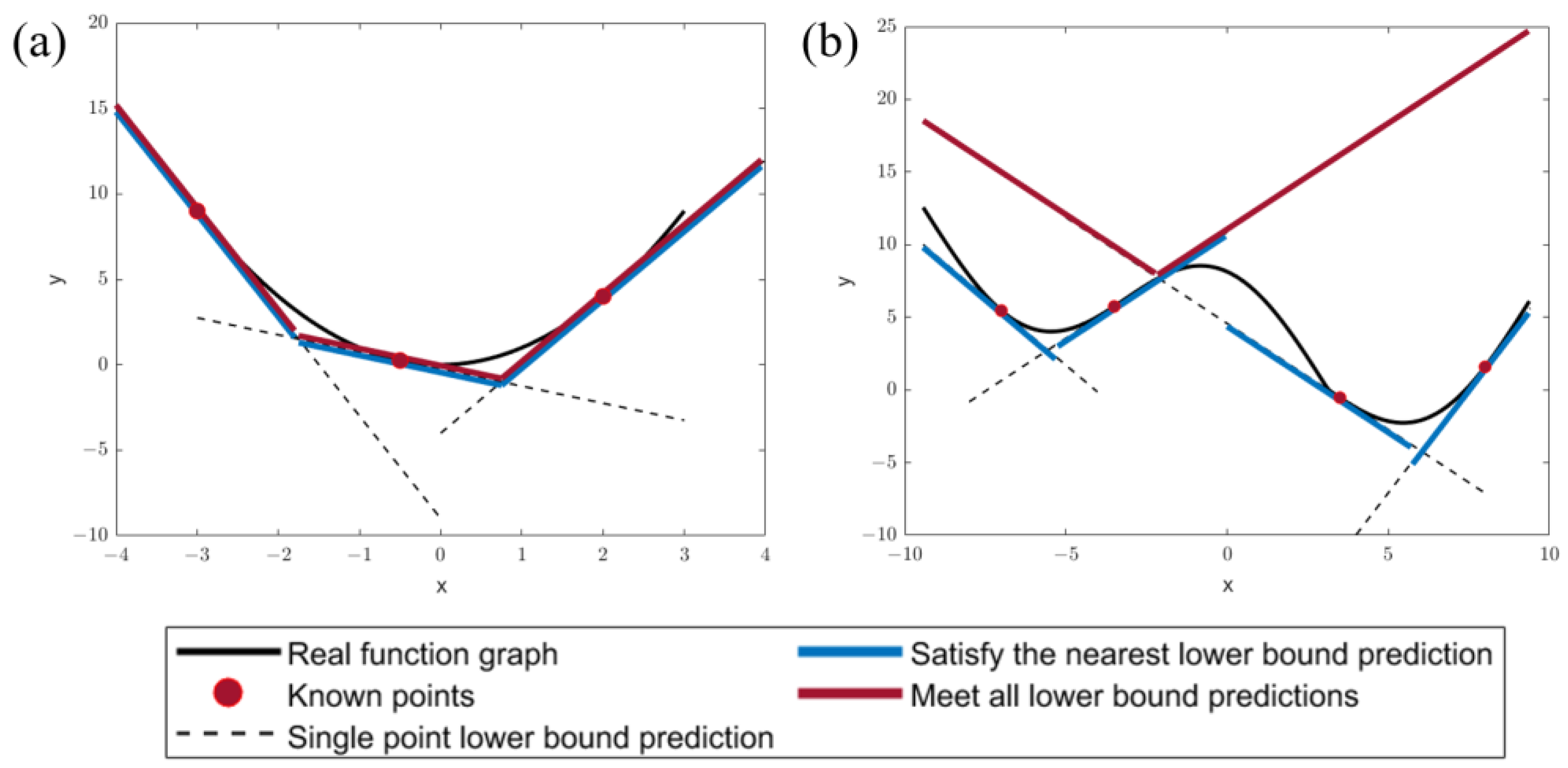
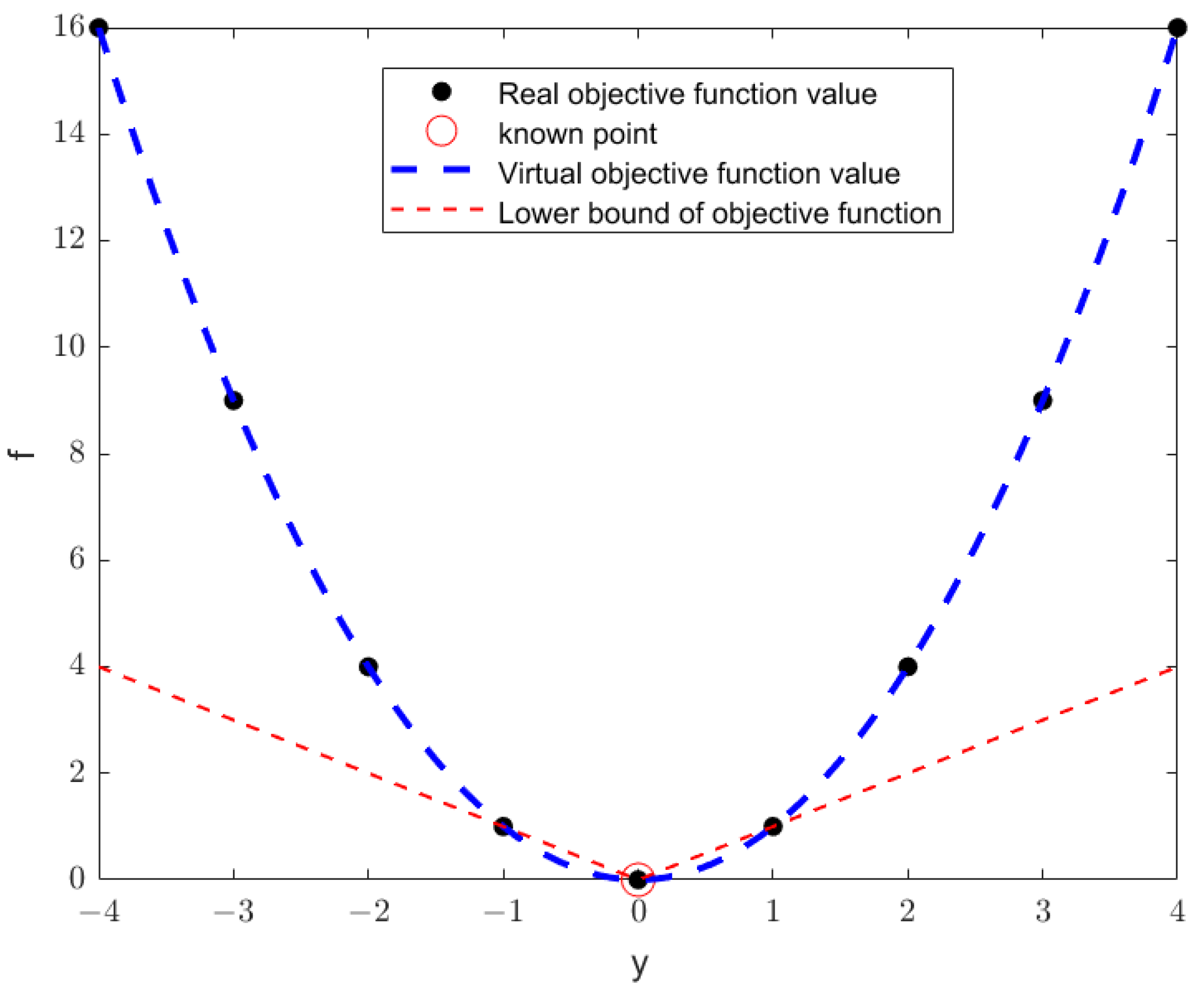
2.2. Proximity Principle and Logic-Based Proximity Principle Bender’s Decomposition Algorithm

NLP subproblems can obtain global optimal solutions through a multi-start strategy, and its expression is the same as Formulas (4)–(6). The so-called proximity principle aims to avoid MILP solutions from becoming stuck in local optima by controlling the use of Formulas (8) and (9), with its GDP expressed as follows:

$$\mathit{y}=\arg \min \left\{f_{MILP}=\alpha +M\sum _{m\in {\mathcal{N}}_2}{\beta }_m\right\}$$

(18)

Subject to the following:

$$\left[\begin{array}{c}{z}_n\\ K_n\left(\mathit{y},{\mathit{y}}_{\mathit{n}}^{\mathrm{*}},{\mathit{n}}_{\mathit{p}},B_{p,q},q\right)\le \alpha \\ W_{m,n}\left(\mathit{y},{\mathit{y}}_{\mathit{n}}^{\mathrm{*}},{\mathit{n}}_{\mathit{p}},B_{p,q},q\right)\le {\beta }_m\end{array}\right]\bigvee \left[\begin{array}{c}\neg z_n\\ -inf\le \alpha \\ -inf\le {\beta }_m\end{array}\right]$$

(19)

$${\mathsf{\Omega }}_{\mathrm{P}\mathrm{r}\mathrm{o}\mathrm{x}\mathrm{i}\mathrm{m}\mathrm{i}\mathrm{t}\mathrm{y}-\mathrm{p}\mathrm{r}\mathrm{i}\mathrm{n}\mathrm{c}\mathrm{i}\mathrm{p}\mathrm{l}\mathrm{e}}(z_n)=True$$

(20)

$$y_p=\sum _{q=1}^{y_p^{ub}-y_p^{lb}+1}\left(y_p^{lb}+q-1\right)B_{p,q}$$

(21)

$$\sum _{q=1}^{y_p^{ub}-y_p^{lb}+1}{B}_{p,q}=1$$

(22)

$$\sum _{p\in {\mathcal{N}}_3}{B}_{p,y_{p,n}^{\mathrm{*}}-y_p^{lb}+1}\le \dim \left(\mathit{y}\right)-1$$

(23)

$$\begin{gathered} {\mathit{y}}^{\mathit{l}\mathit{b}}\le \mathit{y}\le {\mathit{y}}^{\mathit{u}\mathit{b}},\mathit{y}\in {\mathbb{N}}^{\dim \left(\mathit{y}\right)} \\ \alpha ,{\beta }_m\in \mathbb{R},{\beta }_m\ge 0,B_{p,q}\in \left\{\mathrm{0,1}\right\},z_n\in \left\{False,Ture\right\} \\ m\in {\mathcal{N}}_1,p\in {\mathcal{N}}_2,n\in {\mathcal{N}}_3 \end{gathered}$$

Formulas (18)–(23) and Formulas (7)–(15) differ only in sub-Formulas (8) and (9) and sub-Formulas (19) and (20). Formula (19) involves the definition of a set of disjunctions, corresponding to conditional lower bound estimation of different known points, for which Formulas (8), (9), (13) and (14) are defined. Each disjunction involves only two terms, corresponding to the selection or not of lower bound estimation from a known point ${\mathit{y}}_{\mathit{n}}^{\mathit{*}}$ ($z_n$). The so-called proximity principle defines the interrelationship between $z_n$, expressed as Formula (20), which restricts $z_n=True$ to only the one or few known points with the closest Euclidean distance, while other $z_n=False$. Specifically, use the big-M method to reformulate the Formulas (19) and (20) as follows:

$$\mathit{y}=\arg \min \left\{f_{MILP}=\alpha +M\sum _{m\in {\mathcal{N}}_2}{\beta }_m\right\}$$

(24)

Subject to the following:

$$K_n\left(\mathit{y},{\mathit{y}}_{\mathit{n}}^{\mathrm{*}},{\mathit{n}}_{\mathit{p}},B_{p,q},q\right)\le \alpha +M_1(1-z_n)$$

(25)

$$W_{m,n}\left(\mathit{y},{\mathit{y}}_{\mathit{n}}^{\mathrm{*}},{\mathit{n}}_{\mathit{p}},B_{p,q},q\right)\le {\beta }_m+M_1(1-z_n)$$

(26)

$$\left(z_{n_1}-z_{n_2}\right)M_2+\sum _{p\in {\mathcal{N}}_3}{\left({\displaystyle \frac{y_p-y_{p,n_1}}{y_p^{ub}-y_p^{lb}}}\right)}^2\le \sum _{p\in {\mathcal{N}}_3}{\left({\displaystyle \frac{y_p-y_{p,n_2}}{y_p^{ub}-y_p^{lb}}}\right)}^2+M_2$$

(27)

$$\sum _{n\in {\mathcal{N}}_1}{z}_n=K$$

(28)

$$y_p=\sum _{q=1}^{y_p^{ub}-y_p^{lb}+1}\left(y_p^{lb}+q-1\right)B_{p,q}$$

(29)

$$\sum _{q=1}^{y_p^{ub}-y_p^{lb}+1}{B}_{p,q}=1$$

(30)

$$\sum _{p\in {\mathcal{N}}_3}{B}_{p,y_{p,n}^{\mathrm{*}}-y_p^{lb}+1}\le \dim \left(\mathit{y}\right)-1$$

(31)

$$\begin{gathered} {\mathit{y}}^{\mathit{l}\mathit{b}}=\left[y_p^{lb}\right]\le \mathit{y}=\left[y_p\right]=\left[\begin{array}{c}{y}_1\\ ⋮\\ y_{\dim \left(\overrightarrow{\mathit{y}}\right)}\end{array}\right]\le {\mathit{y}}^{\mathit{u}\mathit{b}}=\left[y_p^{ub}\right],\mathit{y}\in {\mathbb{N}}^{\dim \left(\mathit{y}\right)} \\ \alpha ,{\beta }_m\in \mathbb{R},{\beta }_m\ge 0,B_{p,q},z_n\in \left\{\mathrm{0,1}\right\},m\in {\mathcal{N}}_1,p\in {\mathcal{N}}_2,n,n_1,n_2\in {\mathcal{N}}_3 \end{gathered}$$

where $M_1$ and $M_2$ are sufficiently large numbers, and $M_2$ only needs to use the dimension of $\mathit{y}$. $z_n$ is a Boolean variable and $z_n=1$ indicates that the corresponding constraints (8) and (9) of ${\mathit{y}}_{\mathit{n}}^{\mathit{*}}$ is active, otherwise, the constraints will not work. The value of $z_n$ is limited by Formula (27). The use of Euclidean distance to determine the distance between discrete points in Formula (27) is to keep the master problem to linear programming. Although Formula (27) has a quadratic term, the quadratic term will be completely eliminated by addition and subtraction after expansion, so the master problem is still MILP. If the Euclidean distance from the unknown integer combination $\mathit{y}$ to $n_1$-th known integer combination ${\mathit{y}}_{{\mathit{n}}_1}^{\mathit{*}}$ is less than or equal to the Euclidean distance to $n_2$-th known integer combination ${\mathit{y}}_{{\mathit{n}}_2}^{\mathit{*}}$, any combination of $z_{n_1}$ and $z_{n_2}$ can be considered. However, when the Euclidean distance from the unknown integer combination to $n_1$-th known-point ${\mathit{y}}_{{\mathit{n}}_1}^{\mathit{*}}$ is greater than the Euclidean distance to $n_2$-th known integer combination ${\mathit{y}}_{{\mathit{n}}_2}^{\mathit{*}}$, when $z_{n_1}$ is 1, $z_{n_2}$ is not allowed to be 0, that is, when there are known integer combinations closer to the unknown integer combination, information from known integer combinations farther away will not be given priority. The number of known integer combinations information used is limited by Formula (28), Specifically, when $K$ in Formula (28) equals the number of known points, LB-PBD is equivalent to LB-BD. Generally, $K$ is set to 1 to ensure high accuracy. This part of the content will be discussed in Case 2 of Section 3. The meanings of other variables remain the same as Formulas (7)–(15).

Theorem 2. 

With same known points ${\mathit{y}}_{\mathit{n}}^{*}$, The $f_{MILP}$ solved by Formulas (24)–(30) must be less than or equal to the $f_{MILP}$ solved by Formulas (7)–(11).

Proof of Theorem 2. 

The proof of this theorem is presented in the Supporting Information S1. □

Inference 2. 

For cases where the global optimal solution of MILP master problem is within a local convex domain, as long as each local convex domain has at least one known integer combination, LB-PBD can definitely find the global optimal solution.

Proof of Inference 2. 

The proof of this inference is presented in the Supporting Information S1. □

2.3. Delayed Convergence Strategy and Multi-Start Points Strategy

Due to the fact that LB-PBD only changes the way Formulas (8) and (9) take effect, Theorem 1 still applies to LB-PBD. However, in reality, programming problems are not always convex, and even the neighborhood space of the global optimal solution is concave, which will cause LB-PBD to convergence prematurely. If the real problem is a completely concave function, the $f_{MILP}$ constructed by LB-PBD is the envelope hyperplane of the original function, which is always greater than the original function at any position $\mathit{y}$. Assuming no convergence condition is set, the objective function $f_{MILP}$ solved by MILP will monotonically decrease with increasing algebra (readers can follow the proof process of Inference 1 to prove), which is as follows:

$$f_{MILP,n}\ge f_{MILP,n+1}$$

(32)

Note that this is completely opposite to the properties exhibited by convex functions (according to Inference 1), which is as follows:

$$f_{MILP,n}\le f_{MILP,n+1}$$

(33)

Therefore, the convergence idea can be changed to enable the algorithm to cross the concave function region or find the optimal solution within the concave function region. One direct way is to delay convergence strategy, which requires continuous $i$ generations to have the following:

$$f_{MILP}\ge f_{NLP}$$

(34)

Only then do we believe that the algorithm converges. Obviously, $i$ is a hyperparameter related to the problem. If it is known in advance that the programming to be solved is convex, $i$ can be set to 1; If it is known in advance that the global optimal solution of the programming is within a locally convex domain, but there are some concave domains, an additional requirement can be added that $f_{MILP}$ in this $i$ generation is monotonically increasing.

According to Inference 2, for situations where there are multiple local optima, LB-PBD requires sufficient information within the search scope. Therefore, a multi-start points strategy is also indispensable, or in other words, the accuracy of the algorithm is positively improved. This is also a hyperparameter $h$ related to the problem.

The influence of hyperparameters $i$ and $h$ on two strategies will be discussed in Case 1 and Case 2 of Section 3.

2.4. Solver and Simulator Configuration

The LB-PBD algorithm process is described as

Table 1. Pseudo-code of LB-PBD.

The logic-based proximity principle Bender’s decomposition algorithm for mixed-integer nonlinear programming.
S1. Initialization (multi-start points strategy with hyperparameter $h$)
	Initialize $\mathit{h}$ fixed integer combinations ${\mathit{y}}_{\mathit{n}}^{\mathit{*}}$, and their neighborhood $({\mathit{y}}_{\mathit{n}}^{\mathit{*}}-{\mathit{n}}_{\mathit{p}})$ and $({\mathit{y}}_{\mathit{n}}^{\mathit{*}}+{\mathit{n}}_{\mathit{p}})$, solve the nonlinear programming subproblem (Formulas (4)–(6)) for each fixed integer combinations with objective function value $f_n\left({\mathit{y}}_{\mathit{n}}^{\mathit{*}}\right)$, $f_n\left({\mathit{y}}_{\mathit{n}}^{\mathit{*}}-{\mathit{n}}_{\mathit{p}}\right)$ and $f_n\left({\mathit{y}}_{\mathit{n}}^{\mathit{*}}+{\mathit{n}}_{\mathit{p}}\right)$, constraint function value $g_{m,n}\left({\mathit{y}}_{\mathit{n}}^{\mathit{*}}\right)$, $g_{m,n}\left({\mathit{y}}_{\mathit{n}}^{\mathit{*}}-{\mathit{n}}_{\mathit{p}}\right)$ and $g_{m,n}\left({\mathit{y}}_{\mathit{n}}^{\mathit{*}}+{\mathit{n}}_{\mathit{p}}\right)$, and the optimal objective function value $f_{NLP}$. Set $k=1$ and $kk=0$.
S2. Mixed-integer linear programming master problem
	Solve mixed-integer linear programming master problem (Formulas (13)–(15) and (24)–(31) with all solution of nonlinear programming subproblem (Formulas (4)–(6)). The result of solution is ${\mathit{y}}_{\mathit{k}}^{\mathit{*}}$ with optimization objective function value $f_{MILP}$, if $f_{MILP}>f_{NLP}$, set $kk=kk+1$ and continue with S4, else set $kk=0$ and continue with S3.
S3. Nonlinear programming subproblem
	solve the nonlinear programming subproblem (Formulas (4)–(6)) for each fixed integer combinations ${\mathit{y}}_{\mathit{k}}^{\mathit{*}}$ and their neighborhood $({\mathit{y}}_{\mathit{k}}^{\mathit{*}}-{\mathit{n}}_{\mathit{p}})$ and $({\mathit{y}}_{\mathit{k}}^{\mathit{*}}+{\mathit{n}}_{\mathit{p}})$, with objective function value $f_k\left({\mathit{y}}_{\mathit{k}}^{\mathit{*}}\right)$, $f_k\left({\mathit{y}}_{\mathit{k}}^{\mathit{*}}-{\mathit{n}}_{\mathit{p}}\right)$ and $f_k\left({\mathit{y}}_{\mathit{k}}^{\mathit{*}}+{\mathit{n}}_{\mathit{p}}\right)$, constraint function value $g_{m,k}\left({\mathit{y}}_{\mathit{k}}^{\mathit{*}}\right)$, $g_{m,k}\left({\mathit{y}}_{\mathit{k}}^{\mathit{*}}-{\mathit{n}}_{\mathit{p}}\right)$ and $g_{m,k}\left({\mathit{y}}_{\mathit{k}}^{\mathit{*}}+{\mathit{n}}_{\mathit{p}}\right)$, and optimal objective function value $f_{NLP,k}$, if $f_{NLP,k}\le f_{NLP}$, set $f_{NLP}=f_{NLP,k}$. Then set $k=k+1$ and continue with S2.
S4. Convergence judgment (delayed convergence strategy with hyperparameter $i$)
	If $kk\ge i$, end the algorithm, the global optimal solution is the independent variable $(\mathit{x},\mathit{y})$ corresponding to $f_{NLP}$. Else, set $kk=kk+1$ and continue with S3.

:

While the flow chart of LB-PBD applied in simulator-based optimization is shown as Figure 3.

The algorithm starts with the calculation of the NLP subproblem of random $h$ (multi-start points strategy) initial points and their neighborhood points. The NLP is solved by FMINCON in MATLAB 2021b. ASPEN PLUS V8.8 as the simulator is manipulated through the ActiveX interface and the data transmission is completed by MATLAB. The derivative is obtained through the Open Object Model Framework (OOMF)¹². Then GUROBI 11.0 completes the MILP master problem, giving the minimum lower bound $f_{MILP}$ and the next generation of fixed integer variable ${\mathit{y}}_{\mathit{k}}^{\mathit{*}}$. Then the algorithm iterates between NLP and MILP. After each MILP solution, $f_{MILP}$ is compared with the known minimum NLP objective function $f_{NLP}$ until successive $i$ generations (delayed convergence strategy) meet $f_{MILP}\ge f_{NLP}$, and the algorithm terminates. The optimal solution is the independent variable corresponding to $f_{NLP}$.

The results of all NLP will be recorded to prevent waste of time by repeated solving. And the MATLAB programming environment provides the communication platform between all software. All programs run on a workstation with 16 core CPU W-2295,64 GB of memory and GPU A4000. The specific parameters used by each solver, the method of obtaining derivatives in NLP subproblem solving, and the binary interaction parameters used by simulators can be found in Supporting Information S2.

3. Results and Discussion

This section presents three cases to illustrate LB-PBD. Case 1 illustrates the effectiveness of the proximity principle through two different non-convex MINLP numerical examples while also demonstrating the range of use of $M_1$ in Formulas (25) and (26) and the role of hyperparameters in the multi-start points strategy or the delayed convergence strategy. Case 2 aims to further illustrate the advantages of LB-PBD in simulator-based optimization and determine hyperparameters for Case 3. The comparison with LB-BD aims to illustrate the influence of $K$ in Formula (28).

It is worth noting that in simulator-based distillation optimization, the CPU time of NLP has always been the main component because the simulator takes several seconds to run once. Therefore, the number of times the simulator is used to evaluate the algorithm’s computation time, a good algorithm should obtain a high accuracy while also having a low number of simulator activations.

Case 3 demonstrates the process of optimizing extraction distillation using LB-PBD, indicating that MILP has relatively low time consumption and the algorithm has the potential to be applied in simulator-based optimization.

3.1. Case 1—Numerical Experiment

To demonstrate the algorithm’s ability to navigate local optima and saddle points, two test functions have been selected:

$$\begin{gathered} min:f_1\left(x_1,x_2,y_1,y_2\right)=-\sum _{i=1}^2\left(1+{\displaystyle \frac{x_i-15}{100}}\right)\sin \left({\displaystyle \frac{\pi x_i}{10}}\right)-\sum _{i=1}^2\left(1+{\displaystyle \frac{y_i-15}{100}}\right)\sin \left({\displaystyle \frac{\pi y_i}{10}}\right) \\ 0\le x_i\le 30,x_i\in \mathbb{R},0\le y_i\le 30,y_i\in \mathbb{N},i\in \left\{\mathrm{1,2}\right\} \end{gathered}$$

(35)

With the best solution $x_1=x_2=25.0920$ and $y_1=y_2=25$.

$$\begin{gathered} min:f_2\left(x_1,x_2,y_1,y_2\right)=\sum _{i=1}^2\left(y_i^2-40\cos \left({\displaystyle \frac{\pi }{2}}{y}_i\right)\right)-\sum _{i=1}^2\left(\left(x_i-10y_i\right)\sin (\sqrt{\left|x_i-10y_i\right|})\right) \\ -500\le x_i\le 500,x_i\in \mathbb{R},-20\le y_i\le 20,y_i\in \mathbb{N},i\in \left\{\mathrm{1,2}\right\} \end{gathered}$$

(36)

With the best solution $x_1=x_2=-500$ and $y_1=y_2=4$.

Figure 4 illustrates the NLP results of two test functions under all integer combinations. The blue dots in the graph represent the corresponding optimal objective function values under integer combinations. The bluer the surface color, the smaller the value. The multi-start strategy is applied to NLP to prevent solutions from multiple local optima in a fixed integer combination. The number of multi-start points is set to 10 for Formula (35) and 200 for Formula (36), which can ensure the global optimality of the solution.

Notably, there are four locally optimal solutions with significantly different distances in $f_1(y_1,y_2)$, with objective function values differing by less than 1%. While three local optima exist near the global optima integer combinations of $f_2(y_1,y_2)$, with objective function values differing by less than 1%.

In the discussion of algorithm performance below, a solution is considered globally optimal if its final values in each dimension differ from the global optimum by less than 0.1%. To avoid skewed conclusions from random occurrences, each experiment is repeated 100 times, and the average result is taken. The algorithms compared include LB-BD, LB-PBD, and the deterministic benchmark algorithm LB-OA [14], as well as Synchronously Population-Distributed Differential evolution (SPDDE) [32], a stochastic algorithm benchmark.

Firstly, in order to test the approximate range of use of $M_1$ in Formulas (25) and (26), taking the above test functions as examples, with the maximum and minimum difference between the two functions rounded up to ${10}^n$ ($n$ is a positive integer) as the benchmark, $M_1$ is set to ${10}^{n+m}$ ($m$ is also a positive integer), the hyperparameter $h$ of multi-start points strategy is set to 8, and the hyperparameter $i$ of the delayed convergence strategy is set to 3. The accuracy changes with m as shown in Figure 5, with specific data available in Table S4 of the Supporting Information S3. It can be seen that setting $m=2$ no longer affects the normal solution of MILP (fluctuations are caused by random integration phenomena), and an excessively large $m$ will make Formulas (25) and (26) ill-conditioned, not only increasing solution time but also possibly reducing algorithm accuracy.

Secondly, the test results of different algorithms are shown in Figure 6, with specific data available in Tables S2 and S3 of the Supporting Information S3, where LB-BD and LB-PBD used different hyperparameters. LB-PBD showed an increasing trend in algorithm accuracy with the increase of hyperparameters for both strategies in both test functions; however, LB-BD showed a continuous decrease in algorithm accuracy as the hyperparameters of both strategies increased in test function (1) and a very low accuracy in test function (2). This validates our conclusion in Figure 1 and Theorem 2.

Due to $f_1$ being a typical function where continuous and discrete variables can be separated, LB-OA exhibits ultra-high accuracy. However, due to the mixing of the two variables in $f_2$, its accuracy is completely lost. The random algorithm SPDDE is unable to extricate itself from local optima and exhibits poor accuracy because of the fact that $f_1$ has four locally optimal solutions that are far apart. On the other hand, $f_2$ has four locally optimal solutions that are close in distance, which is beneficial for the SPDDE to converge to the global optimal solution as the population shrinks. However, it should be noted that this requires setting appropriate hyperparameters such as population size; otherwise, the accuracy will still be poor (refer to the results in Table S3 of Supporting Information S3). Overall, for unknown MINLP test functions, LB-PBD with reasonable hyperparameters would be a good choice.

A complete example of the calculation process of Formula (35) is described in Appendix A to help readers understand the working principle of LB-PBD.

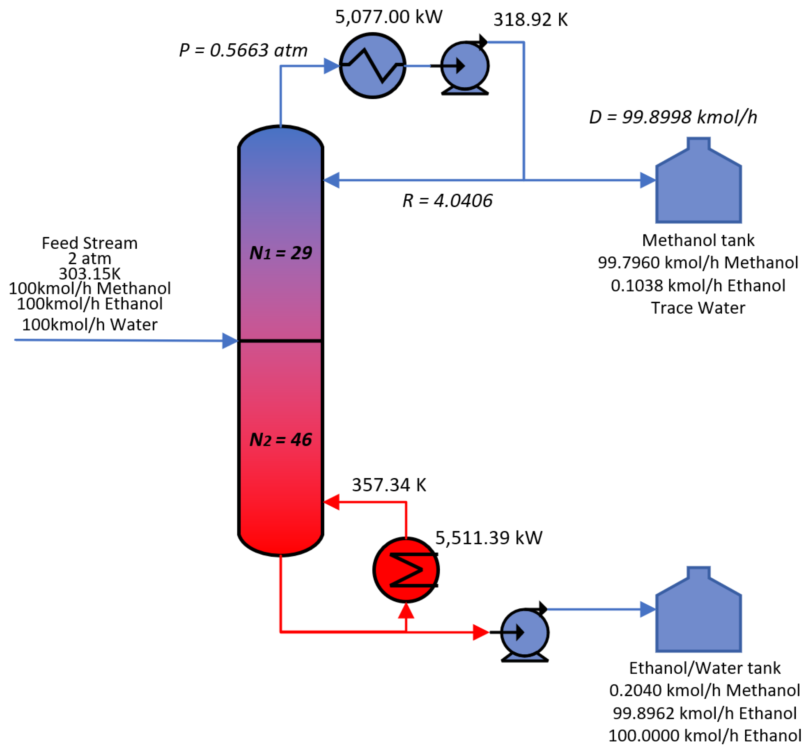
3.2. Case 2—Single Column Case of Methanol Distillation

This case focuses on the optimization of a single distillation column, specifically separating a ternary mixture of methanol, ethanol, and water (with a molar flow ratio of 1:1:1) with a flow rate of 300 kmol/h, shown as Figure 7, where all independent variables are marked. The objective is to achieve a methanol purity of greater than 99.9 mol% at the top of the column, while the methanol purity at the bottom should be less than 0.1 mol%. The minimum TAC and the corresponding design parameters of the distillation column are calculated. The TAC calculation formula is provided in Table S5, and the upper and lower bounds of each independent variable are listed in Table S6.

The global optimal solution for all integer combinations is represented in Figure 8, based on a grid of 19,881 points. The black areas indicate regions where the separation requirements are not met, while the bluer areas correspond to lower TAC values. Figure 8 reveals that, as expected, increasing the number of trays results in for higher pressure, which in turn reduces the amount of steam required within the column, lowering the heat duty. However, contrary to the ideal case, as the number of trays increases, the reflux ratio first decreases and then increases. This occurs because the pressure drop of the column becomes more significant with more trays, leading to greater exergy losses and a more pronounced remixing effect. Consequently, the concentration of ethanol (the light non-key component) at the top of the column increases, requiring a higher reflux ratio to mitigate this. This phenomenon results in the TAC no longer exhibiting convexity for columns with a large number of trays, meaning that the LB-OA algorithm may fail to find the global optimal solution.

This case uses LB-PBD and LB-BD for testing and comparison. Each test is repeated 30 times, and the average results are taken. The detailed test results are presented in Table S7 of Support Information S4. From the data, we can see that LB-PBD, which applies a delayed convergence strategy and a multi-start points strategy, maintains high accuracy. Its MILP consumption time is also within 1 min. In most cases, the global optimal solution can be found within 50 iterations, 200 or fewer NLP subproblems where the problem has nearly 20,000 integer combinations.

The data in

Table 2. Excerpt results of LB-PBD (hyperparameters i = 5 and K = 1).

Hyperparameter h	Average CPU Consumption (Excluding NLP Consumption)/s	Average Number of Iterations	Average Number of NLP Solved	Theoretical Number of NLP Solved Increases
1	39.70	32.9	164.4	-
5	42.23	30.3	171.7	(5 − 1) × 5
15	60.63	26.5	202.7	(15 − 1) × 5

and

Table 3. Comparison of average accuracy.

Hyperparameters	LB-PBD ($\mathit{K}=1$)	LB-PBD ($\mathit{K}=3$)	LB-BD
$i=1,h=5$	28/30	9/30	0/30
$i=1,h=15$	30/30	20/30	0/30
$i=3,h=5$	30/30	22/30	0/30
$i=3,h=15$	30/30	30/30	0/30
$i=5,h=5$	30/30	28/30	0/30
$i=5,h=15$	30/30	30/30	0/30

are excerpted from Table S7, and the trends shown in the tables can also be found on other parameters.

Firstly, according to Table 2, as the hyperparameter $h$ of the multi-start points strategy increases, the number of known points for each MILP master problem increases, and then the time consumption increases. However, the number of iterations decreases, resulting in a smaller increase in the number of NLP subproblems to be solved than the increase in the number of NLP subproblems caused by the multi-start points strategy. Due to the fact that the time consumption of NLP dominates in the actual optimization process, this means that the multi-start points strategy can improve the accuracy of the algorithm while also consuming better time compared to the traditional strategy that optimization is independently executed multiple times. It is worth noting that the multi-start points strategy concentrates NLP, which is beneficial for the deployment of parallel computing.

Secondly, according to Table 3, this conclusion was verified: as the value of $K$ in Formula (28) increases (the reason for setting $K=3$ is that only 3 points are needed to obtain a unique convex hull in two-dimensional space), the performance of LB-PBD tends towards LB-BD. This trend weakens with an increase in the number of known points (multi-start points strategy or delayed convergence strategy), as more known points make programming convex in most of the convex hull, which helps the algorithm to quickly find local optimal solutions. Therefore, if it is predicted that the programming will be convex in a specific area, $K=n+1$ ($n$ is the dimension of the discrete independent variable) can be set to speed up the algorithm. Conversely, when the information of the programming is unknown, $K=1$ should be taken to ensure the high accuracy of the algorithm.

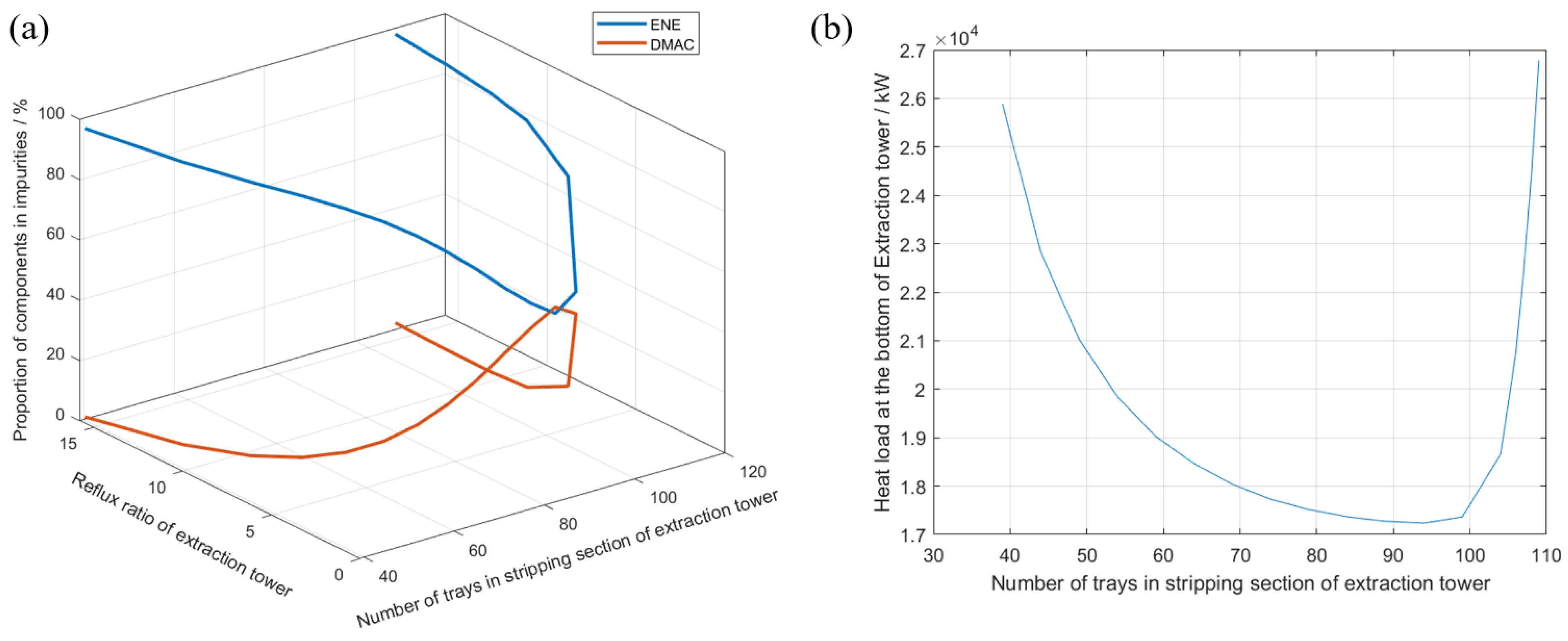
3.3. Case 3—Extraction Distillation Case of Cyclohexane/Cyclohexene

This case is adapted from part of a published work [33] on the separation of a near-azeotropic system composed of cyclohexane (ANE) and cyclohexene (ENE) using extractive distillation. Dimethylacetamide (DMAC) is employed as the entrainer, with its physical properties consistent with the reported properties [33]. A detailed description of the process is provided in the Supporting Information S5, with the search bounds listed in Table S8. The TAC calculation formula is referenced from Table S5.

The hyperparameter $i$ of the delayed convergence strategy is set to 5, the hyperparameter $h$ of the multi-start points strategy is set to 15, and the hyperparameter $K$ in Formula (28) is set to 1. Figure 9a illustrates the time consumption per generation, where each generation includes one set of NLP subproblems and one MILP master problem. Figure 9b depicts the optimizing process of Case 3, while Figure 9c presents the optimal solution found by the algorithm.

Firstly, it is important to note that we cannot conclusively state that the solution obtained is the global optimum, as it has not been validated through exhaustive enumeration, and NLP algorithms cannot guarantee a globally optimal solution. However, as discussed in Section 2, the results sufficiently demonstrate that the solution is “good enough” for practical purposes. Therefore, the current solution is deemed sufficiently “excellent”. Moreover, the lower bound curve obtained by MILP in Figure 9b has multiple obvious inflection points, indicating the existence of multiple local optima in the process, which verifies the algorithm’s ability to cross over local optima. Additionally, for comparison, this case is calculated using SPDDE, and the results are shown in the Supporting Information S5. Unfortunately, in a similar time consumption, the solution obtained by SPDDE is worse than that obtained by LB-PBD, even worse than the most upper bound in LB-PBD.

Secondly, compared to the results from article [33], our optimization yielded a different operational strategy for the extraction column. In that, the column used a high reflux ratio, resulting in ENE being the main impurity at the top of the column. In contrast, by utilizing the NLP search algorithm, we obtained a solution with a lower reflux ratio, which caused DMAC (the heavier entrainer) to be the main impurity at the top, thereby reducing energy consumption and increasing the recovery rate of ENE.

An experiment was designed to explain this phenomenon: the molar purity of ANE was ensured to be 0.999 by changing the reflux ratio of the extraction column, the molar purity of ENE was ensured to be 0.999 by changing the distillate rate at the top of the extraction column, and the number of trays in the stripping section of the extraction column was changed. Other operating parameters were consistent with Figure 9c. The trend of the reflux ratio versus the impurity composition at the top of the extraction column is shown in Figure 10a, and the trend of the heat duty at the bottom of the extraction column is shown in Figure 10b. When the number of trays in the stripping section is small, with the increase of the number of trays in the stripping section, its ability to remove light components increases, and ANE is driven to the top of the column first, which allows the top of the column to use smaller reflux ratios to achieve the purity requirements of ANE, and with the further increase of the number of trays in the stripping section, ENE is driven to the top of the column as well, which makes the top of the column need to use larger reflux ratios in order to clean the excess of ENE. Regardless of the larger or smaller number of trays, the higher high reflux ratios used in the extraction column corresponded to the presence of ENE as the main component in the impurities at the top of the column and a higher heat duty, whereas in the case of smaller reflux ratios there, was a higher amount of DMAC in the impurities as well as a lower heat duty.

This phenomenon can be explained as follows: when the reflux ratio is low, the rectifying section cannot effectively remove the heavy entrainer DMAC near the top of the column, leading to a higher concentration of entrainers in the impurities. As the reflux ratio increases, the separation ability of the rectifying section improves, reducing the entrainer content. However, too much ANE, the primary component in the reflux, dilutes the DMAC, weakening the entrainer’s ability to enhance the relative volatility of the ANE/ENE mixture. Consequently, more ENE enters the top of the column at higher reflux ratios.

Lastly, Figure 9a shows that, in simulation-based optimization, the increase in solving time due to the complexity of MILP is negligible when there are few iterations. This observation suggests that LB-PBD is not only effective but also suitable for simple industrial applications due to its manageable computational requirements. However, the time-consuming nature of MILP increases with the number of iterations, which greatly increases the time-consuming nature of the algorithm when applied in high-dimensional and more complex situations.

4. Conclusions

This work introduces the proximity principle for the MILP master problem in the decomposition algorithm. This principle imposes disjunction constraints on the use of different known integer combination information, ensuring that only the integer combination information with the closest Euclidean distance is used when evaluating the lower bound of unknown combinations.

Applying the proximity principle to the LB-BD algorithm to generate LB-PBD, mathematical analysis, and three case studies have proven that the proximity principle effectively improves the accuracy of the original algorithm. Combined with the multi-start points strategy and delayed convergence strategy, LB-PBD has global optimal convergence for non-convex MINLP.

By employing basis transformation, the Euclidean distance between unknown and known integer combinations is further reduced, improving the accuracy of lower bound predictions. Specifically, the time consumption analysis of Case 3 indicates that the algorithm has the potential to be applied in simulator-based optimization.

However, the significant time consumption in solving the NLP subproblems continues to hinder further advancement of LB-PBD. Meanwhile, Case 3 shows that with the increase of the number of iterations, the solving time of MILP increases, which hinders the application of the algorithm in high-dimensional problems. To address these problems, future research is suggested to focus on integrating stochastic algorithms to reduce the search space of deterministic algorithms, thereby curbing excessive time consumption and enhancing the scalability of the approach for higher-dimensional problems.

References

1. Sorensen, E. Principles of Binary Distillation. Distillation: Fundamentals and Principals; Elsevier: Amsterdam, The Netherlands, 2014; pp. 145–185. [Google Scholar] [CrossRef]
2. David, S.S.; Ryan, P. Lively. Seven chemical separations to change the world. Nature 2016, 532, 435–437. [Google Scholar] [CrossRef]
3. Boukouvala, F.; Misener, R.; Floudas, C.A. Global optimization advances in Mixed-Integer Nonlinear Programming, MINLP, and Constrained Derivative-Free Optimization, CDFO. Eur. J. Oper. Res. 2016, 252, 701–727. [Google Scholar] [CrossRef]
4. Storn, R.; Price, K. Differential evolution—A simple and efficient heuristic for global optimization over continuous spaces. J. Glo. Opt. 1997, 11, 341–359. [Google Scholar] [CrossRef]
5. Hu, Z.; Li, P.; Liu, Y. Enhancing the Performance of Evolutionary Algorithm by Differential Evolution for Optimizing Distillation Sequence. Molecules 2022, 27, 3802. [Google Scholar] [CrossRef] [PubMed]
6. Clerc, M.; Kennedy, J. The particle swarm—Explosion, stability, and convergence in a multidimensional complex space. IEEE Trans. Evol. Comp. 2002, 6, 58–73. [Google Scholar] [CrossRef]
7. Liang, M.; Song, J.; Zhao, K.; Jia, S.; Qian, X.; Yuan, X. Optimization of dividing wall columns based on online Kriging model and improved particle swarm optimization algorithm. Comp. Chem. Eng. 2022, 166, 107978. [Google Scholar] [CrossRef]
8. Holland, J.H. Adaptation in Natural and Artificial Systems; MIT Press: Cambridge, UK, 1976. [Google Scholar] [CrossRef]
9. Zhang, D.; Zeng, S.; Li, Z.; Yang, M.; Feng, X. Simulation-assisted design of a distillation train with simultaneous column and sequence optimization. Comp. Chem. Eng. 2022, 164, 107907. [Google Scholar] [CrossRef]
10. Zhang, X.; Jin, L.; Cui, C.; Sun, J. A self-adaptive multi-objective dynamic differential evolution algorithm and its application in chemical engineering. Appl. Soft Comp. 2021, 106, 107317. [Google Scholar] [CrossRef]
11. Xu, Z.; Ding, Y.; Ye, Q.; Li, J.; Wu, H.; Pan, J. Investigation of side-stream extractive distillation for separating multi-azeotropes mixture based on multi-objective optimization. Chem. Eng. Proce. Proc. Inten. 2024, 200, 109793. [Google Scholar] [CrossRef]
12. Aspen OOMF—Script Language Reference Manual; AspenTech: Knowledge Base; Aspen Technology, Inc.: Bedford, MA, USA, 2011.
13. López, C.A.M.; Telen, D.; Nimmegeers, P.; Cabianca, L.; Logist, F.; Van Impe, J. A process simulator interface for multiobjective optimization of chemical processes. Comp. Chem. Eng. 2018, 109, 119–137. [Google Scholar] [CrossRef]
14. Milán-Yañez, D.; Caballero, J.A.; Grossmann, I.E. Rigorous design of distillation columns: Integration of disjunctive programming and process simulators. Ind. Eng. Chem. Res. 2005, 44, 6760–6775. [Google Scholar] [CrossRef]
15. Lawler, E.L.; Wood, D.E. Branch-and-Bound Methods: A Survey. Oper. Res. 1966, 14, 699–719. [Google Scholar] [CrossRef]
16. Geoffrion, A.M. Generalized Benders decomposition. J. Optim. Theory Appl. 1972, 10, 237–260. [Google Scholar] [CrossRef]
17. Duran, M.A.; Grossmann, I.E. An outer-approximation algorithm for a class of mixed-integer nonlinear programs. Math. Prog. 1986, 36, 307–339. [Google Scholar] [CrossRef]
18. Tapio, W.; Frank, P. An extended cutting plane method for solving convex MINLP problems. Comp. Chem. Eng. 1995, 19, 131–136. [Google Scholar] [CrossRef]
19. Ugray, Z.; Lasdon, L.; Plummer, J.; Glover, F.; Kelly, J.; Martí, R. Scatter Search and Local NLP Solvers: A Multistart Framework for Global Optimization. INFORMS J. Comput. 2007, 19, 328–340. [Google Scholar] [CrossRef]
20. Trespalacios, F.; Grossmann, I.E. Review of Mixed-Integer Nonlinear and Generalized Disjunctive Programming Methods. Chem. Ingen. Tech. 2014, 86, 991–1012. [Google Scholar] [CrossRef]
21. Su, L.J.; Grossmann, I.E.; Tang, L.X. Computational strategies for improved MINLP algorithms. Comp. Chem. Eng. 2015, 75, 40–48. [Google Scholar] [CrossRef]
22. Franke, M.B. Mixed-integer optimization of distillation sequences with Aspen Plus: A practical approach. Comp. Chem. Eng. 2019, 131, 106583. [Google Scholar] [CrossRef]
23. Javaloyes-Antón, J.; Kronqvist, J.; Caballero, J.A. Simulation-based optimization of distillation processes using an extended cutting plane algorithm. Comp. Chem. Eng. 2022, 159, 107655. [Google Scholar] [CrossRef]
24. Bergamini, M.L.; Aguirre, P.; Grossmann, I.E. Logic-based outer approximation for globally optimal synthesis of process networks. Comp. Chem. Eng. 2005, 29, 1914–1933. [Google Scholar] [CrossRef]
25. Gurobi Optimization, LLC. Gurobi Optimizer Reference Manual. 2024. Available online: https://www.gurobi.com (accessed on 22 February 2025).
26. Chia, D.N.; Duanmu, F.; Sorensen, E. Optimal Design of Distillation Columns Using a Combined Optimization Approach. Comp. Aided Chem. Eng. 2021, 50, 153–158. [Google Scholar] [CrossRef]
27. Liñán, D.A.; Contreras-Zarazúa, G.; Sanchez-Ramírez, E.; Segovia-Hernández, J.G.; Ricardez-Sandoval, L.A. A hybrid deterministic-stochastic algorithm for the optimal design of process flowsheets with ordered discrete decisions. Comp. Chem. Eng. 2024, 180, 108501. [Google Scholar] [CrossRef]
28. Caballero, J.A. Logic hybrid simulation-optimization algorithm for distillation design. Comp. Chem. Eng. 2015, 72, 284–299. [Google Scholar] [CrossRef]
29. Trespalacios, F.; Grossmann, I.E. Lagrangean relaxation of the hull-reformulation of linear generalized disjunctive programs and its use in disjunctive branch and bound. Euro. J. Oper. Res. 2016, 253, 314–327. [Google Scholar] [CrossRef]
30. Corbetta, M.; Grossmann, I.E.; Manenti, F. Process simulator-based optimization of biorefinery downstream processes under the Generalized Disjunctive Programming framework. Comp. Chem. Eng. 2016, 88, 73–85. [Google Scholar] [CrossRef]
31. Liñán, D.A.; Ricardez-Sandoval, L.A. A Benders decomposition framework for the optimization of disjunctive superstructures with ordered discrete decisions. AICHE J. 2023, 69, 18008. [Google Scholar] [CrossRef]
32. Lyu, H.; Cui, C.; Zhang, X.; Sun, J. Population-distributed stochastic optimization for distillation processes: Implementation and distribution strategy. Chem. Eng. Res. Des. 2021, 168, 357–368. [Google Scholar] [CrossRef]
33. Lyu, H.; Li, S.; Yu, X.; Sun, J. Superstructure modeling and stochastic optimization of side-stream extractive distillation processes for the industrial separation of benzene/cyclohexane/cyclohexene. Sep. Purif. Technol. 2021, 257, 117907. [Google Scholar] [CrossRef]
34. Duran, M.A.; Grossmann, I.E. A mixed-integer nonlinear programming algorithm for process systems synthesis. AICHE J. 1986, 32, 592–606. [Google Scholar] [CrossRef]
35. Rathore, R.N.S.; Vanwormer, K.A.; Powers, G.J. Synthesis of distillation systems with energy integration. AICHE J. 1974, 20, 940–950. [Google Scholar] [CrossRef]
36. William, L. Plantwide Dynamic Simulators in Chemical Processing and Control, 1st ed.; CRC Press: Boca Raton, FL, USA, 2002. [Google Scholar] [CrossRef]
37. Seider, W.D.; Lewin, D.R.; Seader, J.D.; Widagdo, S.; Gani, R.; Ng, K.M. Product and Process Design Principles: Synthesis, Analysis and Evaluation, 4th ed.; John Wiley & Sons: New York, NY, USA, 2019. [Google Scholar]
38. Luyben, W.L. Principles and Case Studies of Simultaneous Design, 1st ed.; John Wiley & Sons: New York, NY, USA, 2011. [Google Scholar] [CrossRef]
39. Luyben, W.L. Capital cost of compressors for conceptual design. Chem. Eng. Proce. Proce. Inten. 2018, 126, 206–209. [Google Scholar] [CrossRef]
Figure 1. Illustration of different lower bound prediction methods in different functions. (a) A convex function; (b) a non-convex function.
Processes 13 00977 g001
Figure 2. An explanation case of Formula (13).
Processes 13 00977 g002
Figure 3. Architecture of logic-based proximity principle Bender’s decomposition algorithm.
Processes 13 00977 g003
Figure 4. Graph of the NLP results under all integer combinations. (a) Test function f 1 x 1 , x 2 , y 1 , y 2 ; (b) test function f 2 x 1 , x 2 , y 1 , y 2 .
Processes 13 00977 g004
Figure 5. Big-M test results.
Processes 13 00977 g005
Figure 6. Comparison of average accuracy.
Processes 13 00977 g006
Figure 7. Process flow diagram of Case 2.
Processes 13 00977 g007
Figure 8. TAC for different integer combinations.
Processes 13 00977 g008
Figure 9. The test results of Case 3. (a) the time consumption result (b) the process of LB-PBD optimization (c) the optimal solution found by LB-PBD.
Processes 13 00977 g009
Figure 10. Sensitivity analysis of the number of trays in the stripping section of an extracting column: (a) the result of reflux ratio and composition of impurities; (b) the result of heat duty.
Processes 13 00977 g010