AI-Driven Stacking Ensemble for Predicting Total Power Output of Wave Energy Converters: A Data-Driven Approach to Renewable Energy Processes

Abstract

This study develops and evaluates an AI-driven stacked hybrid machine learning model for predicting the total power output of wave energy converters (WECs) across four Australian coastal locations: Adelaide, Perth, Sydney, and Tasmania. This research enhances prediction accuracy through advanced ensemble learning techniques while addressing spatial variability in wave energy processes. The dataset comprises spatial coordinates and power output readings from 16 fully submerged WECs per location, capturing the variability of wave energy across different coastal regions. Data preprocessing included missing value imputation, duplicate removal, and spatial feature transformation via Euclidean distance calculation. Principal component analysis (PCA) was employed to reduce dimensionality while preserving critical features influencing power generation. To develop an accurate prediction model, we employed a stacking ensemble approach using XGBoost, LightGBM, and CatBoost as base learners, optimized via Optuna hyperparameter tuning with 10-fold cross-validation. A Ridge regression meta-learner combined the outputs of these models, leveraging their complementary strengths to enhance predictive performance. Experimental results demonstrate that the hybrid model consistently outperforms individual models, enhancing predictive accuracy across all locations. Sydney exhibited the highest accuracy (RMSE = 9089.58 W, R² = 0.8576), while Tasmania posed the greatest challenge (RMSE = 45,032.37 W, R² = 0.8378). The ensemble approach mitigated overfitting and improved generalization by leveraging the complementary strengths of XGBoost, LightGBM, and CatBoost. By leveraging AI-driven ensemble learning, this study provides a scalable and reliable framework for wave energy forecasting, facilitating more efficient grid integration and resource planning in renewable energy systems.

1. Introduction

Wave energy, also known as ocean wave power, is a promising renewable energy resource generated by the movements of ocean waves. Unlike solar and wind energy, which are intermittent, wave energy offers greater consistency due to the continuous motion of waves, making it an attractive option for sustainable power generation [1]. Additionally, waves carry significantly more energy per unit area than other renewable energy sources, and with oceans covering nearly 70% of Earth’s surface, they present vast, untapped potential for energy extraction [2].

Wave energy is harnessed using wave energy converters (WECs), which capture wave motion and convert it into electrical power. These converters are classified into point absorbers, oscillating water columns, attenuators, and oscillating wave surge converters [3]. Among these, point absorbers are widely deployed due to their ability to function efficiently under various sea conditions. The captured wave motion is transformed into mechanical energy, which then drives a generator and the generator produces electricity [4].

A major challenge in forecasting the total power output of WECs lies in the highly dynamic and location-dependent nature of ocean conditions. Power output varies significantly based on wave height, frequency, and the spatial positioning of WECs within an array. Accurate forecasting models will be helpful in optimizing energy storage, grid integration, and economic feasibility. However, the existing physical simulation methods are computationally expensive and lack real-time adaptability [5].

WECs are designed to capture and convert the ocean wave energy into electrical power. Their working principle involves harnessing the kinetic and potential energy of waves, typically through mechanical motion, which is then transformed into electricity through electric generator [6]. As waves move across the ocean surface, WECs positioned at or near the water’s surface interact with them. The rising and falling movement of waves causes components of the WEC such as a buoy or piston to move, thereby capturing this energy [7]. The captured wave movements are first converted into mechanical energy by the WEC’s moving parts (e.g., pistons, hydraulic rams, or rotating arms). This mechanical energy is then transferred to a generator, where it is converted into electrical power [8]. This process is commonly performed through linear generators, which utilize the up and down movement of a buoy to produce electrical output. Alternatively, rotational generators use turbines or hydraulic systems to generate power from rotational movement. The generated electrical power is transmitted to the shore via underwater cables and subsequently integrated into the power grid for distribution.

Different types of WECs include point absorbers, oscillating water columns (OWCs), attenuators, and oscillating wave surge converters [9]. This study focuses on point-absorber-type WECs, which are floating devices that oscillate vertically with wave motion and are deployed in arrays. Each point absorber will independently operate, aligning with the multi-output power structure and their output power is recorded in the dataset.

In this study, we used a CETO-based dataset, representing a fully submerged, three-tether point absorber wave energy converter (WEC) developed by Carnegie Clean Energy, an Australian company specializing in renewable energy. CETO devices are fixed to the seabed by three cables, which transfer the captured wave energy to onshore or offshore power generation units [10]. Each of the CETO WECs operates independently, with its absorbed power output (P1 to P16) recorded individually in the dataset.

A distinctive feature of CETO WECs is their three-tether system, which allows movement in various directions, heave (up and down), surge (back and forward), and sway (side to side), enabling efficient energy capture from all wave directions. Since CETO operates underwater, it has a minimal environmental footprint [11]. The WECs will not cause noise pollution, are safe for marine life, do not interfere with coastal aesthetics, and remain protected from extreme weather conditions.

Wave energy is inherently intermittent and location dependent, influenced by tides, wind, and ocean currents. Therefore, accurate predictions of wave energy output are essential for grid operators to balance supply and demand [12]. Regression models facilitate total power output prediction, allowing utilities to reduce reliance on fossil-fuel backups during low-energy periods, thereby contributing to the decarbonization of energy systems.

However, wave energy projects involve high capital and operational costs due to the harsh marine environment, making accurate energy yield predictions crucial for improving return on investment (ROI) calculations for investors [13]. By leveraging regression models, uncertainty in power output estimates can be minimized, supporting robust financial planning.

Although CETO WECs are optimized for minimal interference and maximum energy capture through evolutionary optimization techniques, there are compelling reasons to develop machine learning-based regression models for predicting total power output. Current optimization methods used for positioning CETO devices are computationally expensive, often requiring several minutes or more per evaluation [14]. In contrast, a regression model provides a fast, scalable, and cost-effective alternative, predicting total power output based on WEC positions and wave scenarios. This approach reduces dependence on specialized simulation tools and hardware, making predictions more accessible and computationally efficient.

Another significant advantage of machine learning models is their predictive maintenance capability. By anticipating low-output periods or identifying underperforming devices, operators can schedule maintenance during downtime, reducing operational costs and enhancing overall system efficiency [15].

With global efforts toward decarbonizing energy systems, accurate wave energy predictions play a critical role in quantifying its contribution to renewable energy portfolios, thereby supporting evidence-based policy decisions [16]. Prediction models can also enable digital twins of WEC farms, facilitating real-time simulations and risk assessments to optimize system performance [17].

Moreover, real-time power output predictions allow for adaptive energy management strategies, maximizing wave energy capture efficiency under varying ocean conditions [18]. By analyzing wave energy data from multiple locations—Adelaide, Perth, Sydney, and Tasmania—this study provides a comparative understanding of geographic and environmental factors influencing power generation efficiency.

The predictive models developed in this study will be valuable for energy storage planning and grid integration strategies, ensuring a stable and reliable renewable energy supply [19]. Additionally, these models will assist in identifying underperforming WECs, providing actionable insights to optimize hybrid renewable energy systems—which integrate wave energy with offshore wind and tidal energy.

Mohamed K. Hassan et al. focused on developing a predictive machine learning model to estimate wave energy along Egypt’s northern coast, specifically targeting three locations: Alamein, Alexandria, and Mersa Matruh [20]. They predicted wave height (SWH) and wave period using machine learning for the period 2023–2030.

Zhang et al. (2024) developed a predictive model using CNN-BiLSTM-DELA for short-term wave energy forecasting. They utilized the European meteorological dataset ERA5 (1 h intervals covering 8593 observations) for wave height and wave period [21]. The CNN-BiLSTM-DELA model outperformed BiLSTM, CNN, LSTM, GRU, and other models, achieving the lowest mean squared error (MSE) of 0.0396 W and lowest mean absolute percentage error (MAPE) of 3.7361%.

N. K. K. Pani et al. (2021) developed a hybrid machine learning model to accurately forecast wave energy by predicting significant wave height and wave period [22]. The proposed model employs a Stacking Regressor approach, combining the strengths of Extreme Gradient Boosting (XGBoost) and Decision Tree (DT) models. The hybrid model predicts wave height and wave period, which are then used to calculate wave energy flux and wave power output at a site along the North Carolina coast. It demonstrated superior performance compared to individual models, including XGBoost, Decision Tree Regressor, K-Nearest Neighbor (KNN), and Linear Regression, in accurately forecasting wave energy.

Elkhrachy et al. (2023) proposed a novel comparative approach for ocean wave height and energy spectrum forecasting, evaluating semi-analytical and machine learning models to optimize marine operations and wave energy production [23]. The study applied the Sverdrup Munk Bretschneider (SMB) semi-analytical method, Emotional Artificial Neural Network (EANN), and Wavelet Artificial Neural Network (WANN) models using datasets from two regions: the Aleutian Basin and the Gulf of Mexico. The SMB model performed well for daily wave data, with Nash–Sutcliffe Efficiency (NSE) values of 0.62 (Aleutian Basin) and 0.64 (Gulf of Mexico). The WANN model showed better performance for 12-hourly and daily time scales, particularly in capturing large-scale wave behavior. The EANN model excelled in predicting wave characteristics at an hourly resolution, achieving NSE values of 0.60 (Aleutian Basin) and 0.80 (Gulf of Mexico).

Poguluri et al. (2024) described the optimization of asymmetric WECs using supervised regression machine learning (ML) models, including Multi-Layer Perceptron (MLP), Support Vector Regression (SVR), and XGBoost [24]. The study focused on enhancing WEC performance by optimizing key geometric and operational parameters, such as ballast weight, position, damping coefficients, and wave frequency. XGBoost with tuned hyperparameters is the recommended approach for WEC performance optimization due to its high accuracy and efficiency (MAE: 1.217, R² score: 0.995). The study was conducted at a test site in Jeju, South Korea, using wave data from 1979 to 2008.

Kumar et al. (2024) investigated the use of Artificial Neural Networks (ANNs), time-series models, and regression models to forecast wave energy availability at a site in Fiji using wave height and wave period as key inputs [25]. The study compared the performance of the models based on the MSE, RMSE, MAE, MAPE, and R² metrics and benchmarked them against a naïve model. The empirical results demonstrated that the ANN model outperformed both the regression and time-series models, providing superior accuracy and efficiency in forecasting wave energy. The study highlights that accurate wave modeling, combined with impedance matching, can help optimize maximum power generation.

Avila et al. (2023) proposed a simple and direct method for assessing WECs based on historical wave data using Gaussian mixed models and the Monte Carlo method [26]. The approach estimates daily and monthly converted power values and their confidence intervals, helping to evaluate WEC performance at specific sea locations. The study validated the model using data from two buoys in Gran Canaria and Las Palmas Este, showing that predictions aligned with observed wave patterns and power output. Key findings include the superior performance of the Oyster WEC due to its hydraulic turbine design and the significance of considering the stochastic nature of waves when designing wave power systems. The Monte Carlo simulations effectively modeled uncertainties, highlighting that expected values may not always meet energy demands, necessitating backup systems.

Jun Umeda et al. (2024) proposed a data-driven reactive control strategy for WECs using Gaussian process regression (GPR) and experimentally validated its effectiveness [27]. The GPR model predicts the dynamic behavior of WECs based on input/output motion data, bypassing the need for traditional system identification tests. The study demonstrated that their proposed control strategy accurately predicted position and velocity under both training and testing wave conditions, ensuring stable performance even when wave conditions varied beyond the training set.

Xie et al. (2013) provided a comprehensive review of control strategies for Ocean Wave Energy Converters (OWECs), covering key technologies and challenges in the field of wave energy harvesting [28]. The study explored various classical and modern control techniques, such as latching control, declutch control, reactive control, model predictive control, and state-space control. It discussed their application across three major OWEC types: oscillating-body converters (point absorbers, attenuators, terminators), oscillating water columns (OWCs), and overtopping devices.

Ouyang et al. (2024) proposed a wave-height forecasting (WHF) method using a Gaussian process regression (GPR) approach that integrates uncertainty quantification through Bayesian inference [29]. The study emphasizes the importance of reliable wave-height forecasting for enhancing marine renewable energy exploitation and improving maritime safety.

The existing literature extensively covers predictive modeling for wave energy estimation, wave height forecasting, and the optimization of WECs. Various machine learning methods have been employed, including ANNs, hybrid models (Stacking, CNN-BiLSTM-DELA, GPR), and supervised learning techniques (XGBoost, LightGBM, CatBoost). However, most previous studies focus on single-location datasets or short-term forecasting models. Our proposed work addresses the gap in comprehensive studies by evaluating the spatial variation of wave energy potential across multiple geographically distinct locations, specifically Adelaide, Perth, Sydney, and Tasmania, using a uniform machine learning framework. This multi-location perspective helps identify site-specific optimization potential and inter-regional energy variability.

While studies such as Pani et al. (2021) [22] and Poguluri et al. (2024) [24] have applied individual machine learning models (XGBoost, SVR, ANN)/hybrid approaches, they have not fully explored the potential of a robust ensemble model integrating XGBoost, LightGBM, and CatBoost. Our work bridges this gap by leveraging ensemble learning and hyperparameter tuning to improve prediction accuracy and model stability, as evidenced by the superior performance of the hybrid model, with consistently high R² values across test sets.

Our study stands out by evaluating wave energy potential across four distinct coastal regions of Australia. This multi-location analysis provides valuable insights into site-specific power generation potential, spatial energy variability, and regional WEC deployment optimization, offering scalable solutions for regional energy planning. The integration of XGBoost, LightGBM, CatBoost, and an ensemble hybrid model optimized through 10-fold cross-validation represents a novel approach that significantly enhances prediction accuracy. Unlike previous research that primarily focused on individual models (e.g., XGBoost or ANN), our study systematically combines and benchmarks hybrid models for wave energy prediction across multiple regions.

To enhance model interpretability, we applied dimensionality reduction techniques such as PCA to identify the most significant features influencing power generation. By reducing dataset complexity, PCA highlights influential WEC positions, improves prediction accuracy, and provides novel insights into optimal WEC placement across regions.

This study aims to develop and compare hybrid machine learning models for predicting total power output from WEC arrays across four real-world wave energy scenarios in Australia: Adelaide, Perth, Sydney, and Tasmania. Through a comprehensive evaluation of hybrid models and feature contributions, our work lays the foundation for efficient regional WEC deployment and energy optimization.

The major contributions of this research work are:

• A novel AI-driven stacking ensemble model integrating XGBoost, LightGBM, and CatBoost with Ridge regression as a meta-learner has been developed to enhance the prediction accuracy of total power output from wave energy converters (WECs).
• Spatial feature transformation using Euclidean distance has been applied to improve model interpretability while preserving critical spatial information.
• Principal component analysis (PCA) has been applied for dimensionality reduction, ensuring efficient feature selection without compromising predictive performance.
• The hyperparameters have been optimized using Optuna with 10-fold cross-validation, ensuring robust model performance and improved generalization across different datasets.
• A comprehensive evaluation has been conducted across four geographically distinct coastal locations (Adelaide, Perth, Sydney, and Tasmania) to analyze the spatial variability of wave energy forecasting.
• The superior performance of the hybrid ensemble model compared to individual models has been demonstrated, with the lowest RMSE and highest R² across all locations, particularly Sydney (RMSE = 9089.58 W, R² = 0.8576) and Tasmania (RMSE = 45,032.37 W, R² = 0.8378).

2. Methodology

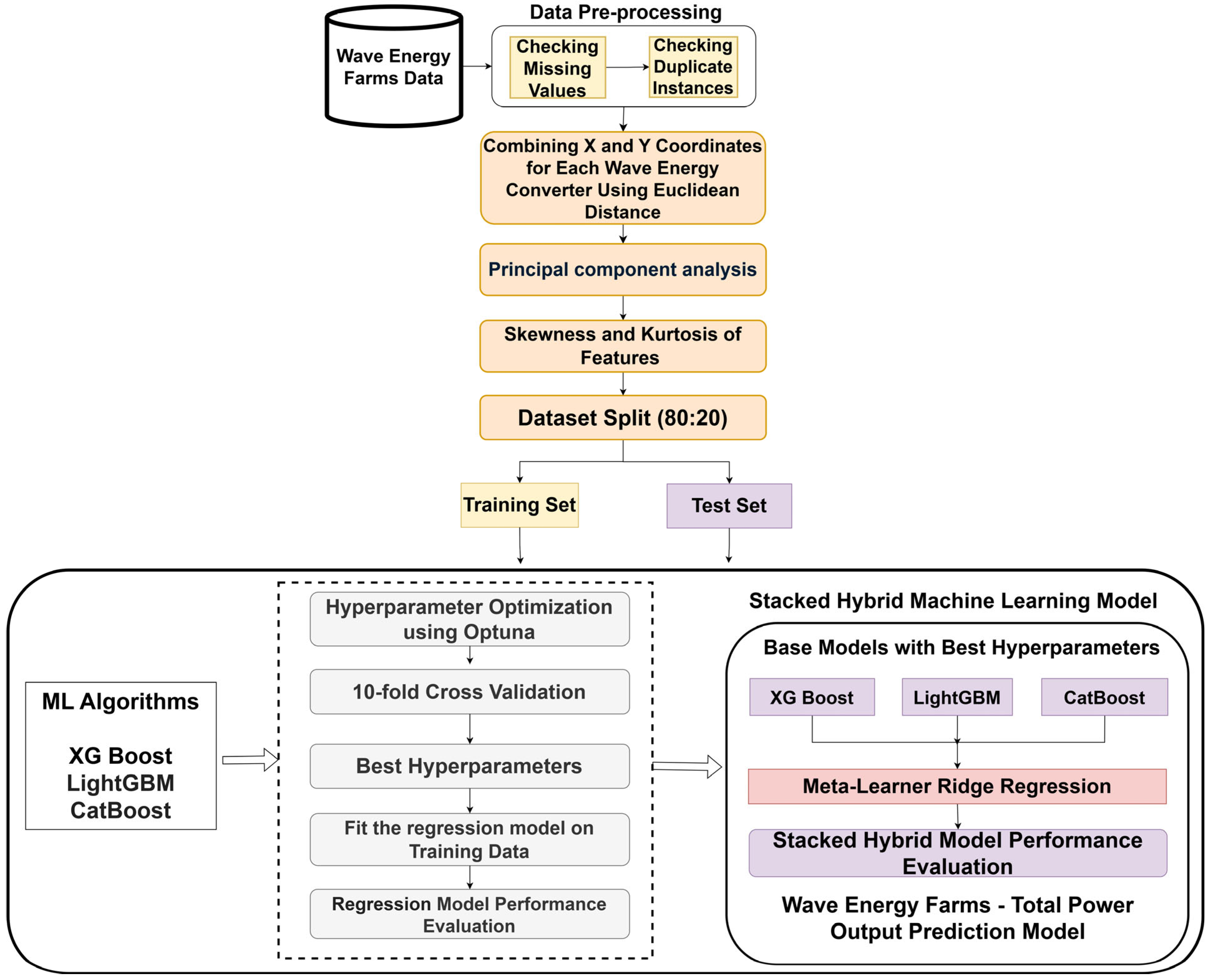
Figure 1 shows the proposed framework for a stacked hybrid machine learning model used to predict the total power output of wave energy farms across the geographically distinct coastal regions of Adelaide, Perth, Sydney, and Tasmania. The wave energy farms dataset undergoes an initial preprocessing phase, which involves checking for missing values to ensure data integrity and checking for duplicate instances to avoid redundancy and improve model accuracy. The X and Y coordinates for each WEC have been combined using the Euclidean distance to calculate the distance from the origin or reference point. This process creates 16 new features (Location1 to Location16) derived from pairs of X and Y coordinates for the 16 WECs. PCA is applied to reduce dimensionality and identify key features influencing power output. Skewness and kurtosis analysis is performed on the features to evaluate data distribution and detect outliers. The dataset is then split into an 80:20 ratio for training and testing, ensuring proper model evaluation.

The framework involves three machine learning algorithms: XGBoost, LightGBM, and CatBoost. Hyperparameter optimization using Optuna, a powerful search framework for tuning parameters, is performed for all the ML algorithms. Additionally, 10-fold cross-validation is conducted to evaluate and select the best-performing hyperparameters for each base model. The optimized base models (XGBoost, LightGBM, and CatBoost) are stacked, with their outputs serving as inputs to a meta-learner Ridge regression model. This ensemble approach leverages the strengths of each model, enhancing prediction accuracy and stability.

The stacked hybrid model is evaluated on both the training and test wave energy datasets. Metrics such as Mean Absolute Error (MAE), Root Mean Squared Error (RMSE), Mean Squared Error (MSE), and R² are used to assess performance.

2.1. Data

In this study, we utilized a CETO-based dataset, representing the operational data from a fully submerged three-tether point absorber WEC developed by Carnegie Clean Energy, an Australian company known for its innovative contributions to renewable energy [30]. The CETO system is distinct from conventional surface wave energy devices due to its fully submerged design, which enhances reliability and minimizes visual and environmental impact. The dataset includes power output readings from 16 individual CETO WEC units, denoted as P1 to P16. Each unit operates independently, with its absorbed power output recorded separately, enabling the analysis of both individual and aggregated performance.

The wave energy farm datasets are collected from four geographically distinct coastal locations in Australia: Adelaide, Perth, Sydney, and Tasmania. Each dataset initially contains 49 features (columns) and a large number of data instances: Adelaide has 71,999 instances, Perth has 72,000 instances, Sydney has 72,000 instances, and Tasmania has 72,000 instances.

The dataset includes pairs of X and Y coordinates (e.g., X1, Y1, X2, Y2, etc.), representing the positions of individual WECs within the wave farm. This spatial configuration allows for the analysis of how the placement of WECs affects wave energy absorption. The power output readings, denoted as P1 to P16, correspond to the 16 individual WEC units, with each providing independent power output measurements. These measurements facilitate the evaluation of spatial and operational variability across the four geographically distinct locations (Adelaide, Perth, Sydney, and Tasmania).

The total power output serves as the target variable for this model and is derived by aggregating the power output from all 16 WEC units (P1 to P16). This allows for a comprehensive assessment of wave energy farm performance and optimization potential across different regions.

2.2. Data Pre Processing

For wave energy farm total power prediction using the hybrid ensemble model (stacking ensemble with XGBoost, LightGBM, and CatBoost), high-quality and well-preprocessed data are critical. Preprocessing is necessary to address issues like missing data, incomplete records, and redundancy, which can introduce biases, inconsistencies, and errors during model training, ultimately leading to inaccurate predictions [31]. By ensuring only complete and consistent data instances are used, preprocessing improves the efficiency and accuracy of machine learning models.

One of the key steps in preprocessing is the removal of redundant or duplicated records, which can otherwise reduce computational efficiency and increase the risk of overfitting [32]. Identifying and eliminating such data improves model performance and ensures reliable predictions. Additionally, preprocessing ensures that features such as X and Y coordinates and individual WEC power outputs (P1 to P16) are accurate, enabling the hybrid models to effectively predict total power output.

After preprocessing, the number of data instances slightly changes across some locations due to the removal of incomplete or inconsistent records. The Adelaide dataset retains 71,999 instances as only minimal cleaning was required. The Perth dataset reduced to 71,758 instances after eliminating 242 data points. The Sydney dataset reduced to 44,826 instances. The Tasmania dataset remains at 72,000 instances, indicating no data issues. By ensuring clean, complete, and consistent data, preprocessing facilitates accurate feature selection, better prediction accuracy, and stable performance in the hybrid ensemble model. This step plays a critical role in minimizing model errors, reducing overfitting, and enhancing the overall reliability of wave energy farm total power predictions across different coastal locations.

2.3. Exploratory Data Analysis

Figure 2a presents a three-dimensional visualization of the relationship between the total power output and the average X and Y positions of the WECs in the Adelaide wave farm. The X-axis represents the average X position of the WECs, and the Y-axis represents the average Y position. The Z-axis (color scale) denotes the total power output, with the color gradient indicating power intensity. Warmer colors (yellow/green) denote higher power outputs, while cooler colors (blue/purple) represent lower outputs. The maximum power output is observed near the coordinates (271.02, 273.65), with a total power of 1,583,052.17 W, marked as “Max Power” in red. The clustering of data points suggests a dense distribution of power values around certain WEC positions, highlighting that placement significantly impacts power generation.

Figure 2b presents a 3D scatter plot depicting the relationship between the spatial positioning of WECs and the corresponding total power output in Perth. A specific point, highlighted at coordinates (250.54, 245.64), shows the maximum recorded power output of 1,565,836.35 W. The color gradient reveals that as the WECs are placed further from the optimal central region, the power output generally declines. This pattern emphasizes the critical role of spatial positioning in wave energy absorption, driven by wave intensity and interference effects.

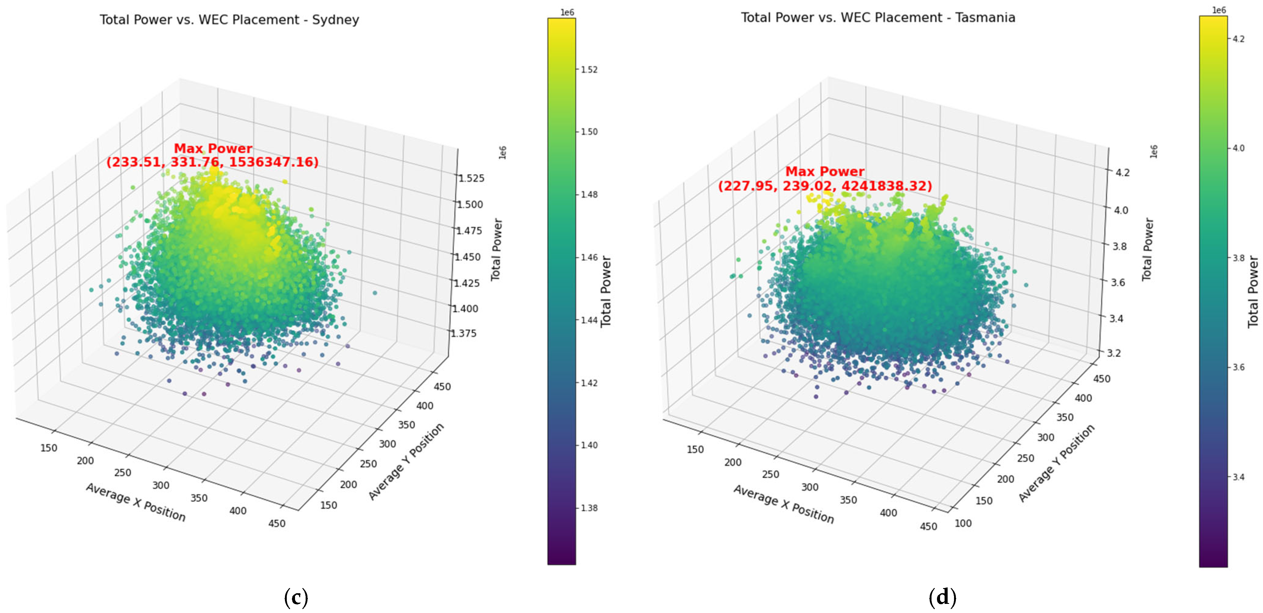
Figure 2c visualizes the relationship between the average X and Y positions of WECs and the total power output for the Sydney wave energy farm. The maximum power output is marked at the coordinates (233.51, 331.76) with a total power of 1,536,347.16 W. The color distribution highlights the importance of precise WEC positioning for efficient wave energy capture.

Figure 2d presents a 3D scatter plot illustrating the relationship between the total power output and WEC placement in the Tasmania wave farm. The highest recorded power output is marked at the coordinates (227.95, 239.02), with a total power of 4,241,838.32 W. The color gradient and distribution of points suggest that optimal placement of WECs significantly influences energy output due to varying wave intensities and interactions among the units.

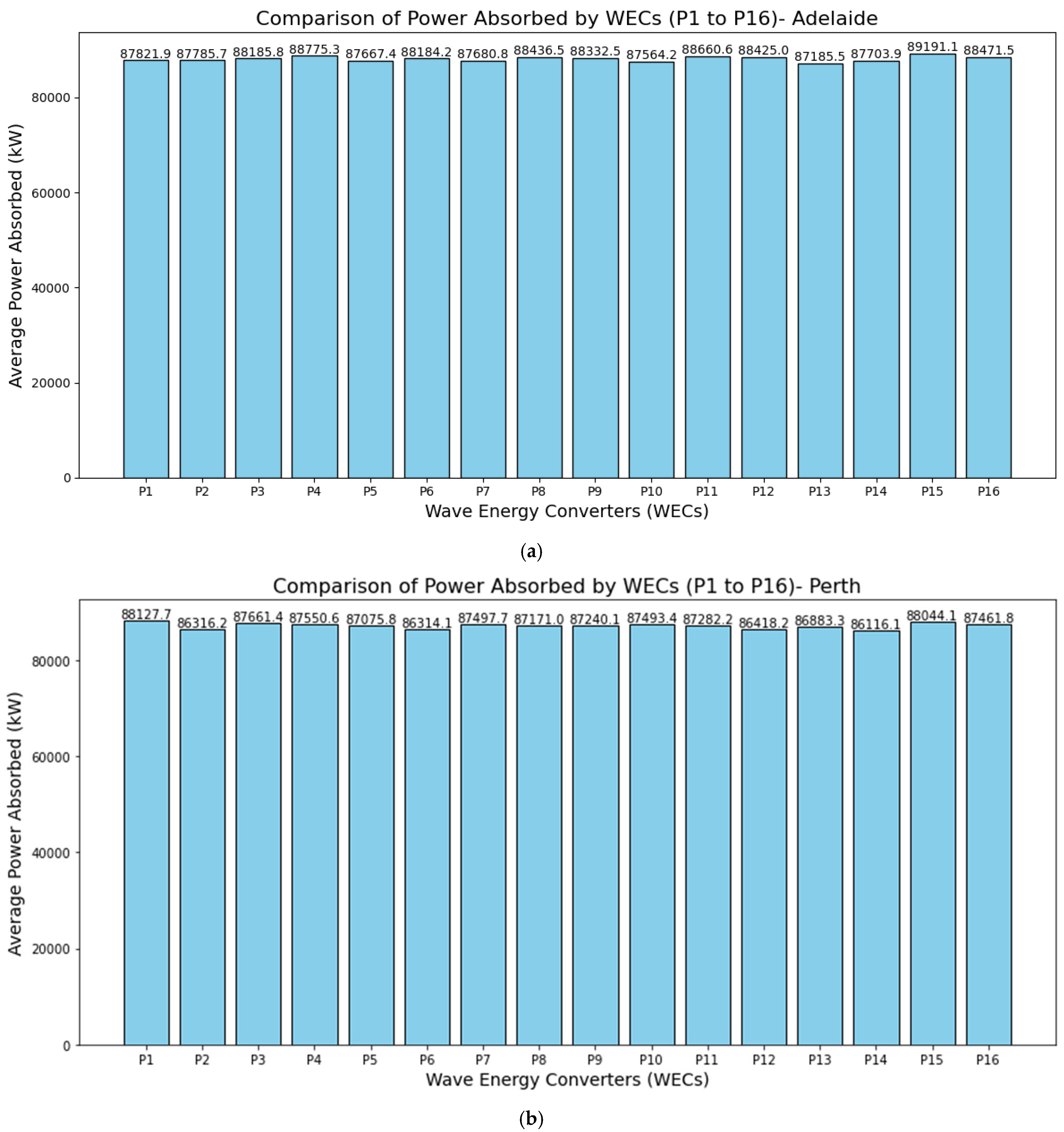
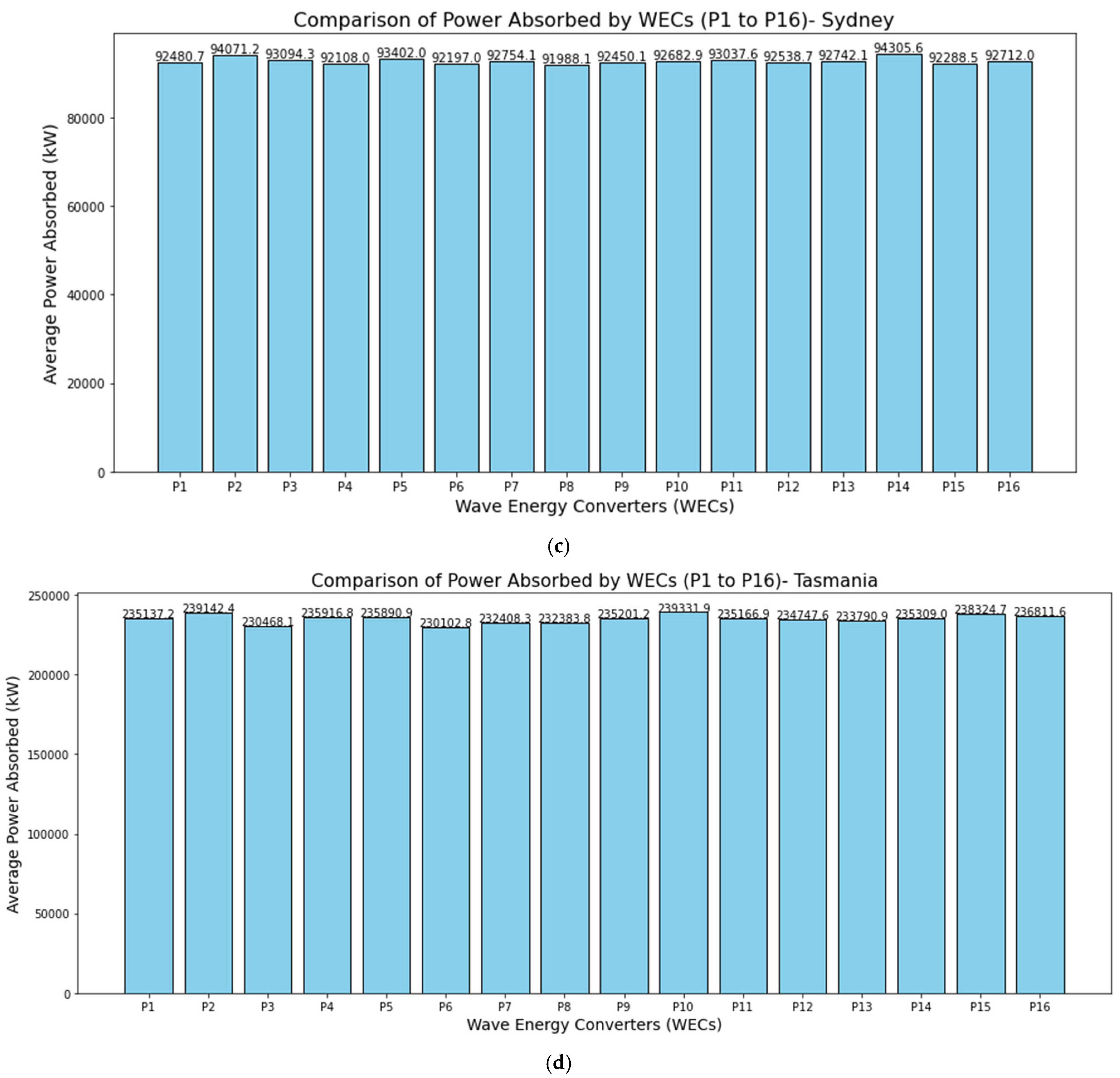
Figure 3 presents a comparison of the average power absorbed by WECs (P1 to P16) at four locations: (a) Adelaide, (b) Perth, (c) Sydney, and (d) Tasmania. Each bar represents the average power absorbed (in W) by an individual WEC, labeled P1 through P16. The plot helps assess how effectively each WEC is converting wave energy into usable power, allowing operators to identify higher or lower performing devices. Identifying WECs with consistently lower power output can pinpoint potential mechanical or operational issues. Early detection enables targeted maintenance or design tweaks to improve efficiency. For Adelaide, the highest recorded average power is for P15 (≈89,191 W), whereas the lowest is for P13 (≈87,185 W). From the bars in the Perth chart, the maximum average absorbed power among the 16 WECs is approximately 88,127.7 W, and the minimum is about 86,116.1 W. For Sydney, the maximum average absorbed power is approximately 94,305.6 W, while the minimum is about 91,988.1 W. Finally, for Tasmania, the maximum average absorbed power is about 239,142.4 W, whereas the minimum is about 230,102.8 W. Adelaide and Perth exhibit a relatively narrow spread between highest and lowest average power values, suggesting that each WEC is performing fairly consistently within those arrays. Sydney shows a slightly larger gap between its maximum and minimum averages, indicating that positional or site-specific factors may cause more variation in power capture there. Tasmania displays the widest range among the four sites, suggesting that wave conditions and WEC placements there yield a larger discrepancy in average absorbed power, potentially due to stronger or more variable wave climates.

2.4. Combining X and Y Coordinates

In the given datasets of all cities, the X and Y coordinates represent the positions of the 16 individual WEC units (denoted as X1, Y1; X2, Y2; …, X16, Y16). Instead of using the separate X and Y values for each WEC, they are combined into a single feature called Location1, Location2, …, Location16 using the Euclidean distance formula [33], as shown in Equations (1) and (2).

The Euclidean distance is the straight-line distance between two points in a 2D plane. If a point in 2D space is given by coordinates (X,Y), the distance of this point from the origin (0,0) or any fixed reference point can be calculated using the Pythagorean theorem, as expressed in Equation (1).

$$\mathrm{D}\mathrm{i}\mathrm{s}\mathrm{t}\mathrm{a}\mathrm{n}\mathrm{c}\mathrm{e}=\sqrt{{\left(\mathrm{X}\right)}^2+{\left(\mathrm{Y}\right)}^2}$$

(1)

This new location feature provides a simplified representation of the WEC’s position within the wave farm and is defined for each WEC as shown in Equation (2).

$${\mathrm{L}\mathrm{o}\mathrm{c}\mathrm{a}\mathrm{t}\mathrm{i}\mathrm{o}\mathrm{n}}_i=\sqrt{{\left({\mathrm{X}}_{\mathrm{i}}\right)}^2+{\left({\mathrm{Y}}_{\mathrm{I}}\right)}^2}$$

(2)

The newly derived features, Location1 to Location16, represent the distance of each WEC from a fixed reference point. This transformation reduces the complexity of the dataset by converting the X-Y coordinate pairs into a single value, simplifying the analysis of the relationship between WEC positions and wave energy farm output.

The placement of WECs in a wave farm can significantly affect energy absorption due to spatial variations in wave intensity and interactions between units. By combining X and Y coordinates into a single feature, we can effectively study these spatial effects and their impact on wave energy absorption.

These newly created location features are used as inputs to the machine learning models, replacing the original 32 features (X1, Y1; X2, Y2; …, X16, Y16). This simplification improves model interpretability while preserving essential spatial information needed to predict the total power output of the wave farm accurately.

2.5. Principal Component Analysis

PCA is a dimensionality-reduction technique that transforms a set of potentially correlated variables into a smaller number of uncorrelated variables called principal components [34]. These components capture most of the variation in the original dataset, with the first few often accounting for the majority of the total variance.

In wave energy prediction, the dataset from four cities contains many features, including multiple WEC outputs and spatial coordinates. Some of these features may be redundant or highly correlated. When a regression model is trained on too many features—particularly those that are noisy or non-informative—it can overfit, learning patterns specific to the training set rather than generalizable relationships [35]. Reducing dimensionality helps mitigate overfitting by focusing on the most significant patterns.

By filtering out dimensions with low variance (often representing noise), PCA improves the model’s signal-to-noise ratio and thus its prediction accuracy [36]. Fewer dimensions typically mean faster training times and lower memory requirements, which is particularly beneficial when tuning models like XGBoost or CatBoost extensively (e.g., via 10-fold cross-validation). By emphasizing the principal components where variation is highest, the regression model more effectively learns the critical relationships driving wave energy outputs.

Feature contributions have been calculated based on the PCA components. The PCA components form an ncomponents * nfeatures array whose entry vi,j is the loading of feature j on principal component i. The explained variance ratio is a vector r of length ncomponents, where each element ri represents the fraction of variance explained by component i.

The contributions are computed as shown in Equation (3).

$${\mathrm{c}\mathrm{o}\mathrm{n}\mathrm{t}\mathrm{r}\mathrm{i}\mathrm{b}\mathrm{u}\mathrm{t}\mathrm{i}\mathrm{o}\mathrm{n}\mathrm{s}}_{\mathrm{j}}={\sum }_{\mathrm{i}=1}^{{\mathrm{n}}_{\mathrm{c}\mathrm{o}\mathrm{m}\mathrm{p}\mathrm{o}\mathrm{n}\mathrm{e}\mathrm{n}\mathrm{t}\mathrm{s}}}\left|{\mathrm{V}}_{\mathrm{i},\mathrm{j}}\right|{\mathrm{r}}_{\mathrm{i}}\hspace{1em}\mathrm{f}\mathrm{o}\mathrm{r} \mathrm{e}\mathrm{a}\mathrm{c}\mathrm{h} \mathrm{f}\mathrm{e}\mathrm{a}\mathrm{t}\mathrm{u}\mathrm{r}\mathrm{e} \mathrm{j}.$$

(3)

Here, PCA components have shape (ncomponents, nfeatures). ${\mathrm{V}}_{\mathrm{i},\mathrm{j}}$ is the loading (coefficient) of feature j on principal component i. $\left|{\mathrm{V}}_{\mathrm{i},\mathrm{j}}\right|$ is the absolute value of that loading. R = (r1, r2, …, $r_{n_{\mathrm{c}\mathrm{o}\mathrm{m}\mathrm{p}\mathrm{o}\mathrm{n}\mathrm{e}\mathrm{n}\mathrm{t}\mathrm{s}}}$)T is the explained variance ratio for each principal component. Consequently, contributions j is the sum of the products of absolute loadings and their respective variance ratios across all principal components i.

2.6. Machine Learning Algorithms

XGBoost, LightGBM, and CatBoost are widely recognized for their superior performance in regression and classification tasks [37,38,39]. Their gradient-boosting framework helps them capture complex, nonlinear relationships that are common in wave energy data. These algorithms naturally handle irregularities such as outliers, missing values, or skewed distributions. This trait is crucial in wave energy forecasting, where environmental readings can fluctuate due to changing ocean conditions. XGBoost uses a highly optimized tree-building process that can manage large datasets efficiently. LightGBM employs histogram-based algorithms and leaf-wise tree growth, reducing memory usage and training time, making it suitable for large-scale wave datasets. CatBoost incorporates efficient GPU training and handles categorical features without extensive preprocessing, improving overall training speed and reducing model complexity. All three algorithms include regularization parameters (e.g., L1, L2) and various tree-pruning techniques. These help maintain generalization quality, an important consideration for real-world energy applications where future wave conditions can vary significantly.

2.7. Hyperparameter Optimization

Model parameters are the internal coefficients or weights that a training algorithm learns from the data. Hyperparameters are external settings—such as max_depth, learning_rate, and n_estimators—that govern how the algorithm learns [40]. Adjusting these can markedly affect a model’s performance. Proper tuning often yields substantial gains, especially for complex models like gradient-boosted decision trees.

Cross-validation (CV) provides a more robust estimate of out-of-sample performance than a single train/test split, leading to more reliable hyperparameter choices [41]. In this study, we performed 10-fold cross-validation to identify the best hyperparameters. In k-fold cross-validation, the training data are divided into k subsets (folds). The model trains on (k − 1) folds and is tested on the remaining fold, cycling through all folds to compute an average score.

The Optuna framework has been employed for hyperparameter optimization in our research. Optuna is an automatic hyperparameter optimization library that uses a Bayesian sampler to select promising values for each hyperparameter within specified ranges [42]. Over multiple “trials,” Optuna refines its sampling strategy based on previous outcomes, searching for the parameter combination that minimizes (or maximizes) a given objective function.

For the evaluation metric, RMSE has been chosen for each machine learning model, and neg_root_mean_squared_error has been used from Python’s library to ensure that “maximizing” the negative score is mathematically equivalent to minimizing RMSE [43].

The RMSE is determined using the Equation (4).

$$\mathrm{R}\mathrm{M}\mathrm{S}\mathrm{E}=\sqrt{{\displaystyle \frac{1}{\mathrm{n}}}{\sum }_{\mathrm{i}=1}^{\mathrm{n}}{({\mathrm{y}}_{\mathrm{i}}-\widehat{{\mathrm{y}}_{\mathrm{i}}})}^2}$$

(4)

where $y_i$ is the observed value, $\widehat{y_i}$ is the predicted value, and n is the number of observations.

The Optuna optimization loop runs the objective function 20 times, each time sampling a new set of hyperparameters. After each trial, Optuna updates its internal model. Once all trials are complete, the best hyperparameters with the lowest RMSE are selected.

2.8. Hybrid Machine Learning Model

A stacking ensemble model has been employed by combining predictions from three gradient-boosted tree models—XGBoost, LightGBM, and CatBoost—using Ridge regression as a meta-model. In stacking, each base learner produces an output for the same input x. Specifically, let, f_K(x) be the prediction from the kth base models such as XGBoost, LightGBM, CatBoost.

If the base learners produce outputs f₁(x), f₂(x), …, f_K(x), their outputs form a feature vector for the meta-learner:

Z(x) = [f₁(x), f₂(x), …, f_K(x)]

(5)

Each fK(x) denotes the prediction from the Kth base model (e.g., XGBoost, LightGBM, or CatBoost) for input x. These K predictions are concatenated into a single vector z(x)

The final prediction becomes

$${\widehat{\mathrm{y}}}_{\mathrm{s}\mathrm{t}\mathrm{a}\mathrm{c}\mathrm{k}}\left(\mathrm{x}\right)=\mathrm{g}\left(\mathrm{z}\left(\mathrm{x}\right)\right)$$

(6)

where g is the meta-model function. In a linear stacking approach, Ridge regression models this relationship as

$${\widehat{y}}_{\mathrm{s}\mathrm{t}\mathrm{a}\mathrm{c}\mathrm{k}}\left(x\right)={\beta }_0+{\sum }_{k=1}^{\mathrm{K}}{\mathsf{\beta }}_{\mathrm{k}}{f}_k\left(x\right)$$

(7)

Ridge regression fits the coefficients {${\mathsf{\beta }}_{\mathrm{k}}\}$ by minimizing the following regularized sum of squared errors:

$${\sum }_{i=1}^n{(y_i-{\widehat{y}}_{\mathrm{s}\mathrm{t}\mathrm{a}\mathrm{c}\mathrm{k}}{(x}_i))}^2+\mathsf{\alpha }{\sum }_{k=1}^{\mathrm{K}}{{\mathsf{\beta }}_{\mathrm{k}}}^2$$

(8)

where yi is the true target value for input xi, and $\mathsf{\alpha }$ is the regularization coefficient. The ℓ2 penalty term $\mathsf{\alpha }\sum {{\mathsf{\beta }}_{\mathrm{k}}}^2$ prevents overfitting by shrinking large model weights, thereby improving generalization. This stacked model leverages the complementary strengths of the base learners, often achieving higher accuracy or better robustness than any single gradient-boosted model on its own.

2.9. Performance Metrics

The performance metrics Mean Absolute Error (MAE), Mean Squared Error (MSE), Root Mean Squared Error (RMSE), and R² score play a crucial role in evaluating model performance, guiding model improvement, and assessing prediction accuracy [44,45]. MAE, RMSE, and MSE are measured in watts (W) as they quantify errors in predicting power output.

The MAE measures the average magnitude of the errors between predicted values and actual values without considering their direction. It is defined as:

$$\mathrm{M}\mathrm{A}\mathrm{E}=\left({\displaystyle \frac{1}{\mathrm{n}}}\right){\sum }_{\mathrm{i}=1}^{\mathrm{n}}\left|{\mathrm{y}}_{\mathrm{i}}-{\hat{\mathrm{y}}}_{\mathrm{i}}\right|$$

(9)

The MSE calculates the average of the squares of the errors between predicted values and actual values. It is more sensitive to large errors compared to MAE. It is given by:

$$\mathrm{M}\mathrm{S}\mathrm{E}=\left({\displaystyle \frac{1}{n}}\right){\sum }_{i=1}^n{\left(y_{\mathrm{i}}-{\hat{\mathrm{y}}}_{\mathrm{i}}\right)}^2$$

(10)

The R² score, or coefficient of determination, measures how well the predicted values approximate the actual values. An R² score of 1 indicates perfect predictions, while a score of 0 means the model explains no variance. It is defined as:

$${\mathrm{R}}^2=1-{\displaystyle \frac{{\sum }_{i=1}^n{\left(y_{\mathrm{i}}-{\hat{\mathrm{y}}}_{\mathrm{i}}\right)}^2}{{{\sum }_{\mathrm{i}}}^{\mathrm{n}}{\left(y_{\mathrm{i}}-\overline{\mathrm{y}}\right)}^2}}$$

(11)

Here, $\overline{\mathrm{y}}$ is the mean (average) of values and $\hat{\mathrm{y}}$ the predicted value of y.

3. Results and Discussion

This research leverages a CETO-based dataset with power output readings from 16 independent WECs at four geographically distinct coastal locations in Australia: Adelaide, Perth, Sydney, and Tasmania. The dataset includes spatial coordinates and power output measurements, facilitating the evaluation of site-specific wave energy variability.

Initially, the dataset from the four coastal regions included 49 input features for each location. These features consisted of spatial coordinates (X1, Y1; X2, Y2; …, X16, Y16), individual power outputs (P1 to P16), and the total power output of the wave energy farm. To simplify the spatial representation of the 16 WECs within the wave farm, the X and Y coordinates for each WEC were combined using the Euclidean distance method. This transformation replaced the 32 spatial features (X1, Y1; X2, Y2; …, X16, Y16) with 16 new features (Location1 to Location16), representing the distance of each WEC from a fixed reference point. This dimensionality reduction preserved key spatial information while reducing the complexity of the dataset and improving model interpretability.

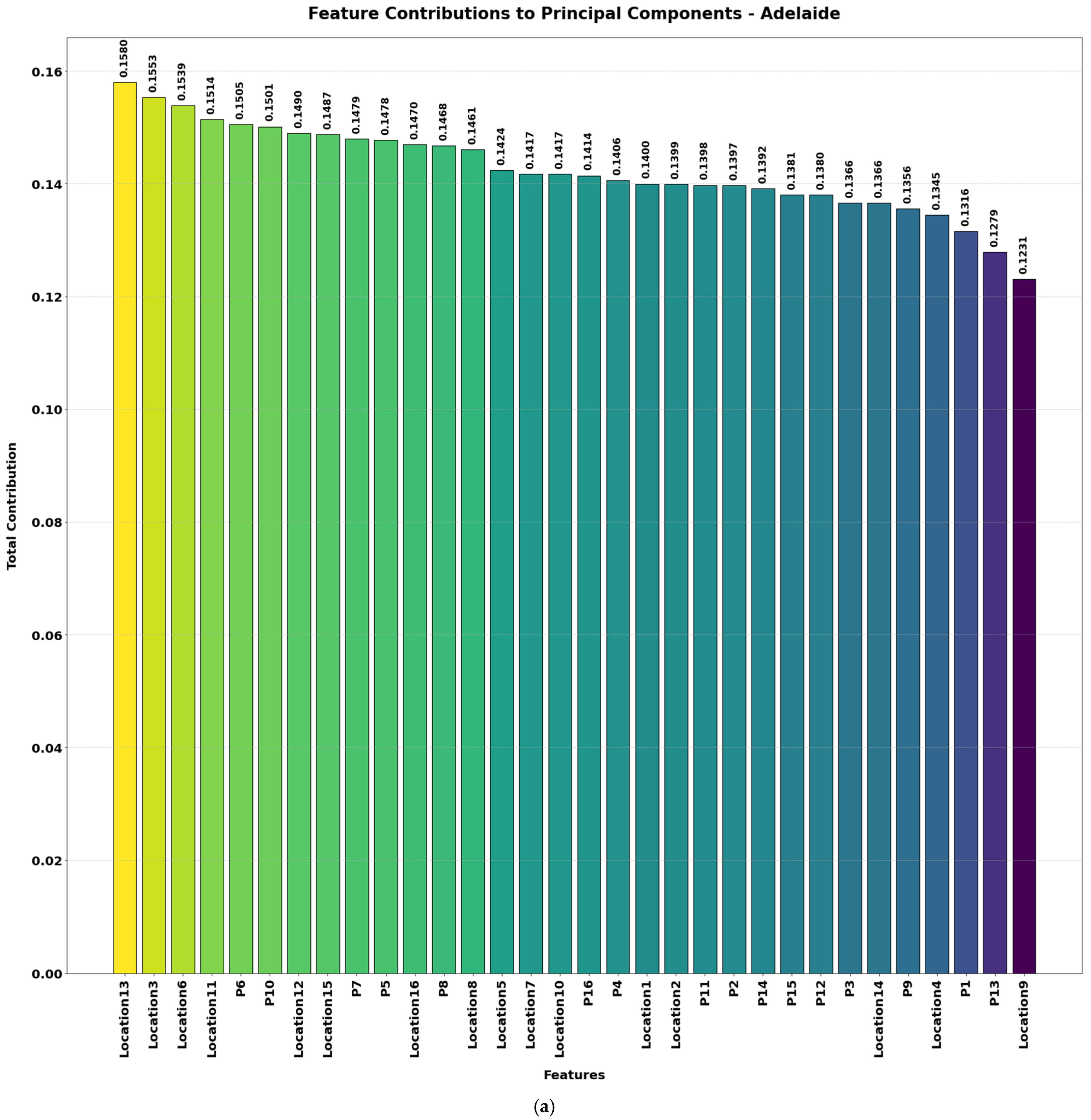
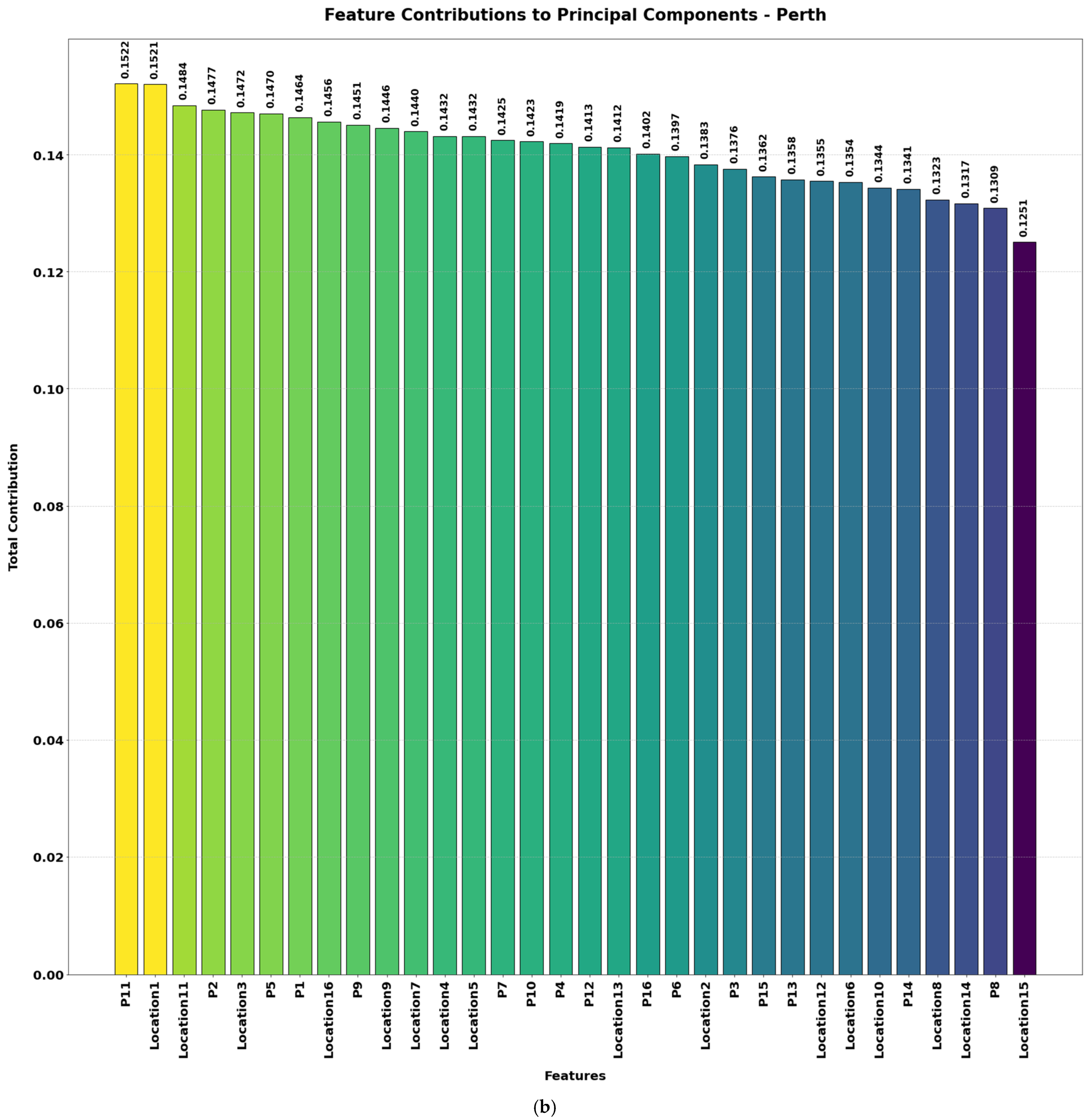
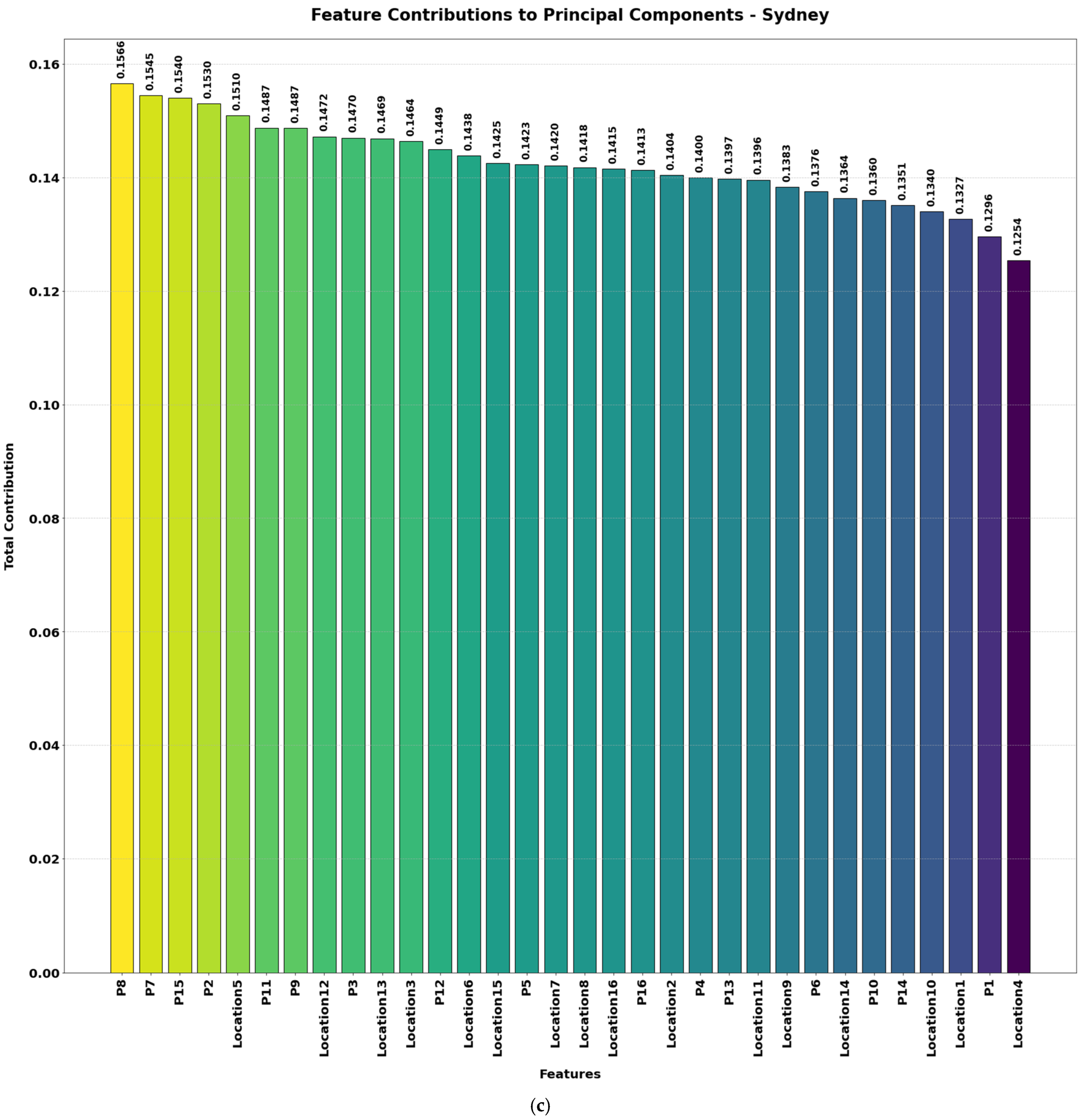
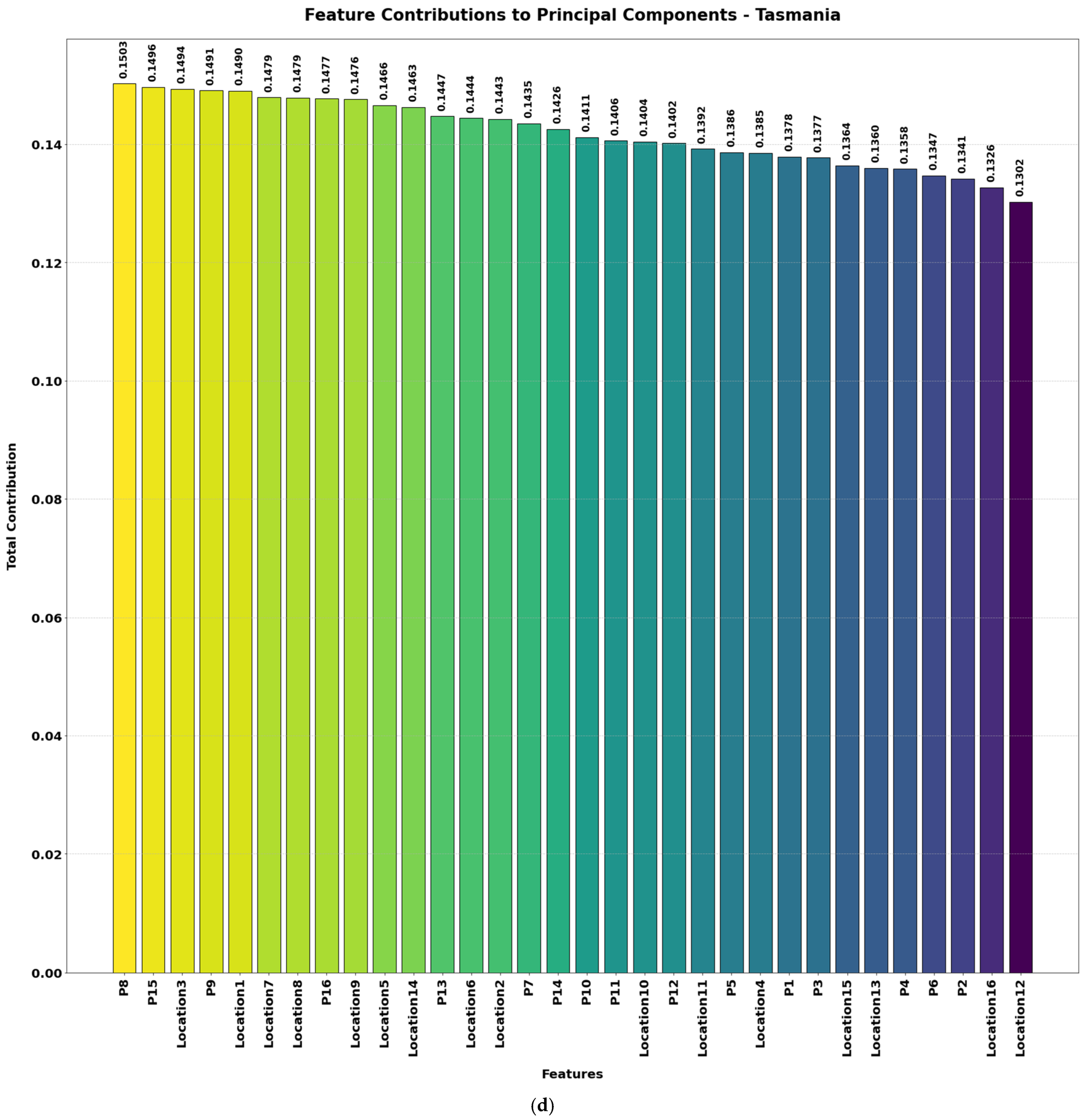
Figure 4a–d illustrate the contributions of various features to the principal components (PCs) used for wave energy prediction across the four locations. These components represent transformations of the original features into a smaller set of uncorrelated variables that capture most of the dataset’s variability. PCA was applied to identify and retain the key features—those contributing the greatest variance—which include both spatial positioning (location features) and power outputs (P1, P2, …). By focusing on these principal components, the model concentrates on the most informative signals for predicting total power output.

By reducing the dataset to 20 essential features, this approach mitigates overfitting, improves interpretability, and accelerates model training—all without sacrificing crucial information related to wave energy generation in Adelaide, Perth, Sydney, and Tasmania. The height of each bar indicates how strongly a given feature influences the principal components, with higher bars signifying greater overall contribution. A higher score for a location feature implies that spatial positioning in that dimension is critical for predicting total power, while a high score for a power feature means that particular WEC output provides essential explanatory power. The inclusion of power features (e.g., P6, P10, P4) shows individual WEC outputs also play a major role in overall energy variation, highlighting the operational differences between these converters.

Table 1. Summary of skewness and kurtosis of features for pre-processed wave energy farms datasets.

Dataset	Adelaide			Perth			Sydney			Tasmania
Raw Dataset	(71,999, 49)			(72,000, 49)			(72,000, 49)			(72,000, 49)
After Preprocessing	(71,999, 20)			(71,758, 20)			(44,826, 20)			(72,000, 20)
Feature	Skewness	Kurtosis	Feature		Skewness	Kurtosis	Feature	Skewness	Kurtosis	Feature	Skewness	Kurtosis
Location 1	−0.33544	−0.39746	Location 1		−0.41902	−0.57397	P8	−0.07613	−0.44327	P8	−0.36284	−0.78317
Location 2	−0.39548	−0.74251	Location 3		−0.46873	−0.54982	P7	−0.04049	−0.3254	P15	−0.61433	−0.60823
Location 3	−0.43011	−0.56175	Location 4		−0.45941	−0.52263	P15	0.152211	−0.59712	Location 3	−0.55304	−0.38626
Location 5	−0.4438	−0.70335	Location 5		−0.34703	−0.30051	P2	−0.21128	−0.72088	P9	−0.43662	−0.80679
Location 6	−0.5782	−0.34341	Location 7		−0.21946	−0.73033	Location 5	−0.32866	−0.85913	Location 1	−0.50354	−0.58078
Location 7	−0.32148	−0.94434	Location 9		−0.4112	−0.58792	P11	0.041975	−0.58869	Location 7	−0.37306	−0.60726
Location 8	−0.34071	−0.42551	Location 11		−0.42636	−0.39101	P9	0.221452	−0.57925	Location 8	−0.34474	−0.63813
Location 10	−0.3518	−0.94475	Location 13		−0.3414	−0.5931	Location 12	−0.48838	−0.34932	P16	−0.56213	−0.60906
Location 11	−0.41941	−0.53315	Location 16		−0.5335	−0.46052	P3	0.029394	−0.6401	Location 9	−0.38603	−0.55933
Location 12	−0.29354	−0.7268	P1		−0.75524	−0.32767	Location 13	−0.51745	0.075147	Location 5	−0.54296	−0.38803
Location 13	−0.36254	−0.49558	P2		−0.46968	−0.70602	Location 3	−0.60046	−0.13881	Location 14	−0.29694	−0.59765
Location 15	−0.36488	−0.5101	P4		−0.65633	−0.5479	P12	−0.10138	−0.61474	P13	−0.42172	−0.81415
Location 16	−0.28409	−0.90798	P5		−0.54662	−0.67001	Location 6	−0.56526	−0.17074	Location 6	−0.40008	−0.78726
P4	−0.68992	−0.51434	P6		−0.46405	−0.67805	Location 15	0.085704	−0.55086	Location 2	−0.44694	−0.39601
P5	−0.58083	−0.62755	P7		−0.6406	−0.49453	P5	−0.05107	−0.48916	P7	−0.34561	−0.88427
P6	−0.59173	−0.62519	P9		−0.6028	−0.55974	Location 7	−0.79511	0.110367	P14	−0.44404	−0.81176
P7	−0.57662	−0.60478	P10		−0.5865	−0.59033	Location 8	−0.66884	−0.10477	P10	−0.69457	−0.56554
P8	−0.68989	−0.4294	P11		−0.54761	−0.66323	Location 16	−0.55691	−0.28547	P11	−0.44938	−0.76847
P10	−0.55059	−0.54424	P12		−0.45261	−0.82581	P16	0.164788	−0.5459	Location 10	−0.31879	−0.71718
P16	−0.66521	−0.59424	P16		−0.65459	−0.56949	Location 2	−0.38459	−0.91852	P12	−0.44077	−0.77784
Total Power	0.299419	−0.34366	Total Power		0.237535	−0.21291	Total Power	−0.34566	−0.2155	Total Power	0.143873	0.237946

provides an overview of skewness and kurtosis values for key features across the four wave energy farm datasets. Initially, each location had 49 features, which were reduced to 20 features after applying PCA. These retained features primarily represent key power outputs (P1 to P16) and spatial locations (Location1 to Location16). The most contributing features to the principal components are shown in Figure 4.

After the preprocessing stage, Adelaide, Perth, Sydney, and Tasmania had 71,999 instances, 71,758 instances, 44,826 instances, and 72,000 instances, respectively. Table 1 lists the features considered for each location, with skewness and kurtosis values falling within acceptable limits. The negative skewness and low kurtosis in many features suggest that the data are well behaved and free of extreme outliers, ensuring stable and reliable model performance.

Table 2. Summary of best hyperparameters for machine learning algorithms (10-fold cross-validation) applied to the wave energy dataset from various Australian cities.

Dataset	ML Algorithm	Best Hyperparameters (10-Fold Cross Validation)
Adelaide	XGBoost	‘max_depth’: 7, ‘learning_rate’: 0.1000850471036407, ‘n_estimators’: 496, ‘subsample’: 0.8949203321429828, ‘colsample_bytree’: 0.8415805819539554
	LightGBM	‘n_estimators’: 414, ‘max_depth’: 7, ‘learning_rate’: 0.07659776218495659, ‘num_leaves’: 50
	CatBoost	‘iterations’: 495, ‘depth’: 9, ‘learning_rate’: 0.09074202931750353, ‘l2_leaf_reg’: 1.6018596082629306, ‘bagging_temperature’: 0.6444867743521498
Perth	XGBoost	‘max_depth’: 7, ‘learning_rate’: 0.06219836832714495, ‘n_estimators’: 449, ‘subsample’: 0.9707611866822229, ‘colsample_bytree’: 0.7743871261533423
	LightGBM	‘n_estimators’: 435, ‘max_depth’: 11, ‘learning_rate’: 0.10280951922892954, ‘num_leaves’: 47
	CatBoost	‘iterations’: 406, ‘depth’: 8, ‘learning_rate’: 0.12096660893670483, ‘l2_leaf_reg’: 5.306157893310288, ‘bagging_temperature’: 0.9804082440121775
Sydney	XGBoost	‘max_depth’: 8, ‘learning_rate’: 0.06001053761605855, ‘n_estimators’: 496, ‘subsample’: 0.9749996181673412, ‘colsample_bytree’: 0.8032849100225273
	LightGBM	‘n_estimators’: 500, ‘max_depth’: 9, ‘learning_rate’: 0.1034242603816564, ‘num_leaves’: 22
	CatBoost	‘iterations’: 437, ‘depth’: 6, ‘learning_rate’: 0.1675309863909748, ‘l2_leaf_reg’: 2.9120299612645275, ‘bagging_temperature’: 0.9212273074957337
Tasmania	XGBoost	‘max_depth’: 7, ‘learning_rate’: 0.06032317126551678, ‘n_estimators’: 463, ‘subsample’: 0.8927501070608183, ‘colsample_bytree’: 0.8278763907002945
	LightGBM	‘n_estimators’: 319, ‘max_depth’: 9, ‘learning_rate’: 0.078590626414356, ‘num_leaves’: 42
	CatBoost	‘iterations’: 457, ‘depth’: 9, ‘learning_rate’: 0.10203410461885462, ‘l2_leaf_reg’: 1.5208211099230344, ‘bagging_temperature’: 0.7792363549885529

presents the best hyperparameters obtained for XGBoost, LightGBM, and CatBoost across four different Australian cities (Adelaide, Perth, Sydney, and Tasmania) after performing 10-fold cross-validation on the wave energy dataset. The selected hyperparameters were optimized to enhance model accuracy and performance in predicting total power output from WECs. Optimized hyperparameters enhance prediction accuracy, ensuring the model generalizes well across different locations. The variation in hyperparameter values across cities reflects differences in wave energy dynamics, dataset size, and noise levels.

Table 3. Performance evaluation of machine learning regression models for predicting total power output.

Dataset	ML Algorithm	Training Set				Test Set
		MAE (W)	MSE (W)	RMSE (W)	R2	MAE (W)	MSE (W)	RMSE (W)	R2
Adelaide	XGBoost	8400.09	130,421,138.81	11,420.20	0.9584	15,296.53	429,725,114.85	20,729.81	0.8637
	LightGBM	12534.78	281,877,093.10	16,789.19	0.9100	15,656.76	439,739,332.96	20,969.96	0.8605
	CatBoost	11547.40	243,456,672.39	15,603.09	0.9223	15,225.46	425,868,117.87	20,636.57	0.8649
	Hybrid model	10667.96	208,122,047.70	14,426.43	0.9336	14,964.68	411,703,252.83	20,290.47	0.8694
Perth	XGBoost	9707.89	165,203,370.12	12,853.14	0.9394	13,333.07	314,615,017.36	17,737.39	0.8843
	LightGBM	9700.02	162,379,364.93	12,742.81	0.9404	13,504.30	322,704,165.47	17,963.96	0.8814
	CatBoost	11279.34	221,424,589.16	14,880.34	0.9187	13,129.44	307,523,494.87	17,536.34	0.8870
	Hybrid model	10211.14	181,926,924.77	13,488.02	0.9332	12,943.94	300,152,158.33	17,324.90	0.8897
Sydney	XGBoost	3369.30	21,160,859.12	4600.09	0.9644	6674.84	85,102,118.98	9225.08	0.8533
	LightGBM	5223.35	49,889,078.36	7063.22	0.9161	6961.57	89,874,101.99	9480.19	0.8451
	CatBoost	5633.05	58,841,577.09	7670.82	0.9010	6793.87	86,564,617.30	9304.01	0.8508
	Hybrid model	4337.39	34,622,264.50	5884.06	0.9418	6601.08	82,620,528.99	9089.58	0.8576
Tasmania	XGBoost	25646.51	1,125,143,703.32	33,543.16	0.9107	35,050.52	2,120,240,714.40	46,046.07	0.8305
	LightGBM	30422.95	1,555,682,114.10	39,442.13	0.8765	35,613.92	2,173,221,085.88	46,617.81	0.8262
	CatBoost	26849.25	1,240,700,572.90	35,223.57	0.9015	34,595.24	2,081,142,914.30	45,619.54	0.8336
	Hybrid model	26255.47	1,180,535,928.02	34,358.92	0.9063	34,203.96	2,027,914,675.17	45,032.37	0.8378

presents the performance metrics of various machine learning models (XGBoost, LightGBM, CatBoost, and a Hybrid model) across four different Australian cities (Adelaide, Perth, Sydney, and Tasmania) for predicting total power output. The models are evaluated using four key metrics for both the training and test sets: Mean Absolute Error (MAE), Mean Squared Error (MSE), Root Mean Squared Error (RMSE), and R-squared (R²) value. MAE, RMSE, and MSE are measured in watts (W) as they quantify errors in predicting power output. Overall, XGBoost outperforms LightGBM and CatBoost in most cases, showing lower RMSE and higher R² scores. However, the Hybrid model consistently delivers the best performance across all cities, demonstrating that stacking models improves prediction accuracy. Among the cities, Sydney exhibits the lowest RMSE and highest R² scores, suggesting less variance and better predictability. Conversely, Tasmania has the highest RMSE and lowest R² scores, indicating greater variability in wave energy outputs and a more challenging prediction task.

For Adelaide, the Hybrid model achieves the lowest test RMSE (20,290.47) and the highest R² score (0.8694), outperforming individual models.

For Perth, the Hybrid model again delivers the best results, with test RMSE = 17,324.90 and R² = 0.8897.

For Sydney, all models perform well, with XGBoost showing the best individual performance (test RMSE = 9225.08, R² = 0.8533). The Hybrid model further improves performance, achieving RMSE = 9089.58 and R² = 0.8576.

For Tasmania, the dataset poses the most challenging prediction task, with higher RMSE values across all models. The Hybrid model again provides the best performance (test RMSE = 45,032.37, R² = 0.8378). Among the base models, XGBoost performs better than LightGBM and CatBoost, though all models struggle with higher variability in total power output.

The Hybrid model consistently achieves the best test set performance across all cities. Stacking multiple gradient-boosted models (XGBoost, LightGBM, and CatBoost) using Ridge regression as a meta-model improves predictive performance. The Hybrid model shows better generalization ability, reducing overfitting compared to individual models. Sydney has the best predictive accuracy, with low RMSE and high R² scores, suggesting more consistent wave energy patterns. Tasmania exhibits the highest RMSE, indicating greater fluctuation in wave energy, making prediction more difficult. Among standalone models, XGBoost performs the best, followed by LightGBM and CatBoost. The Hybrid model is the optimal choice, as it consistently achieves the lowest RMSE and highest R² scores.

While XGBoost, LightGBM, and CatBoost perform well individually, the Hybrid model provides the most accurate predictions overall. Stacking multiple models enhances accuracy and reduces overfitting, making it the most effective approach for predicting total power output from WECs. By leveraging ensemble learning through the Hybrid model, this study demonstrates that combining multiple strong models yields more robust and accurate wave energy predictions across diverse coastal locations in Australia.

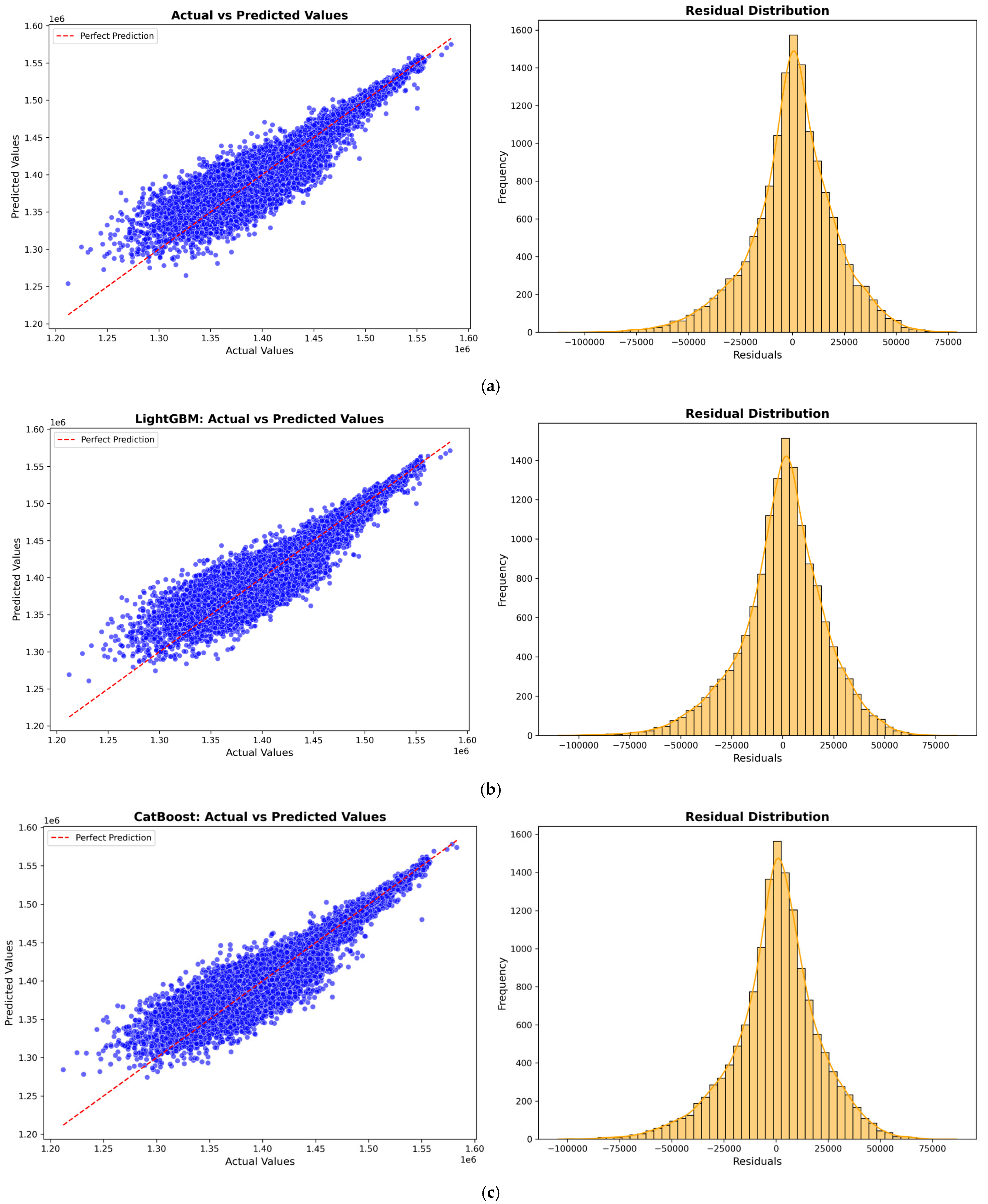
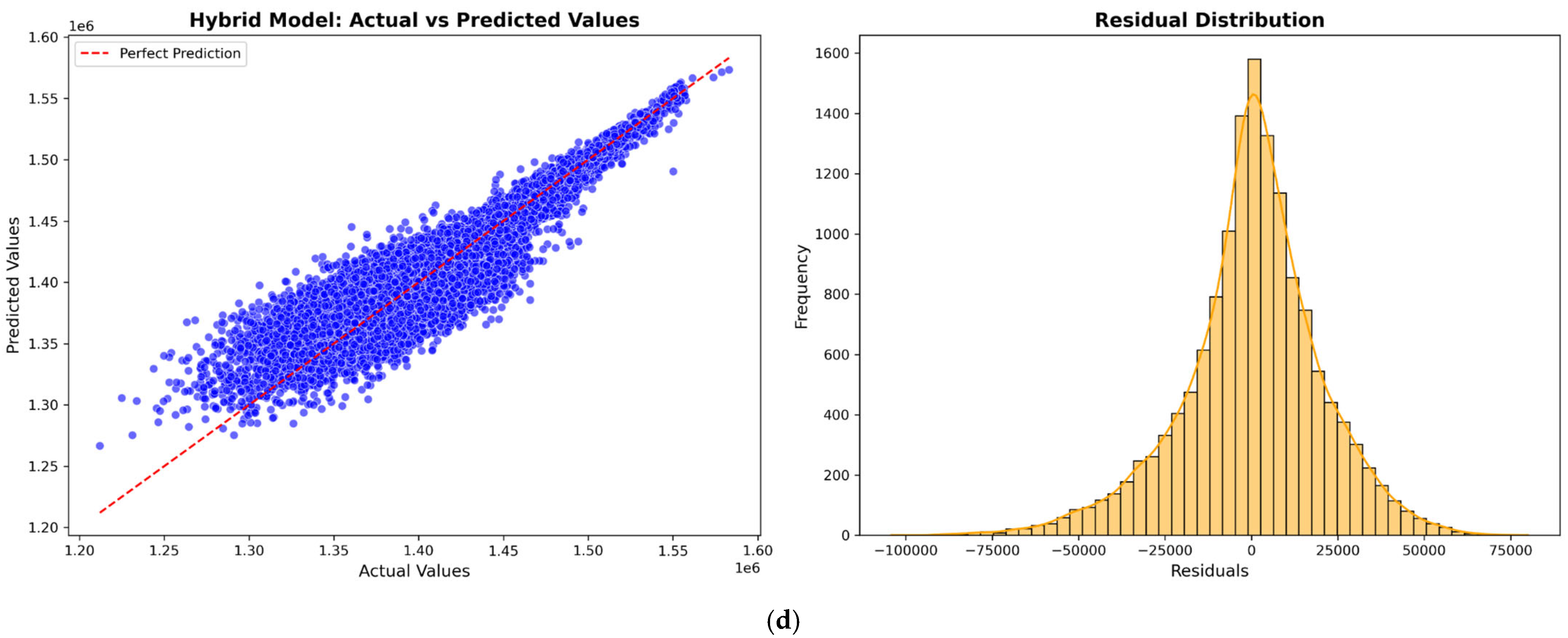
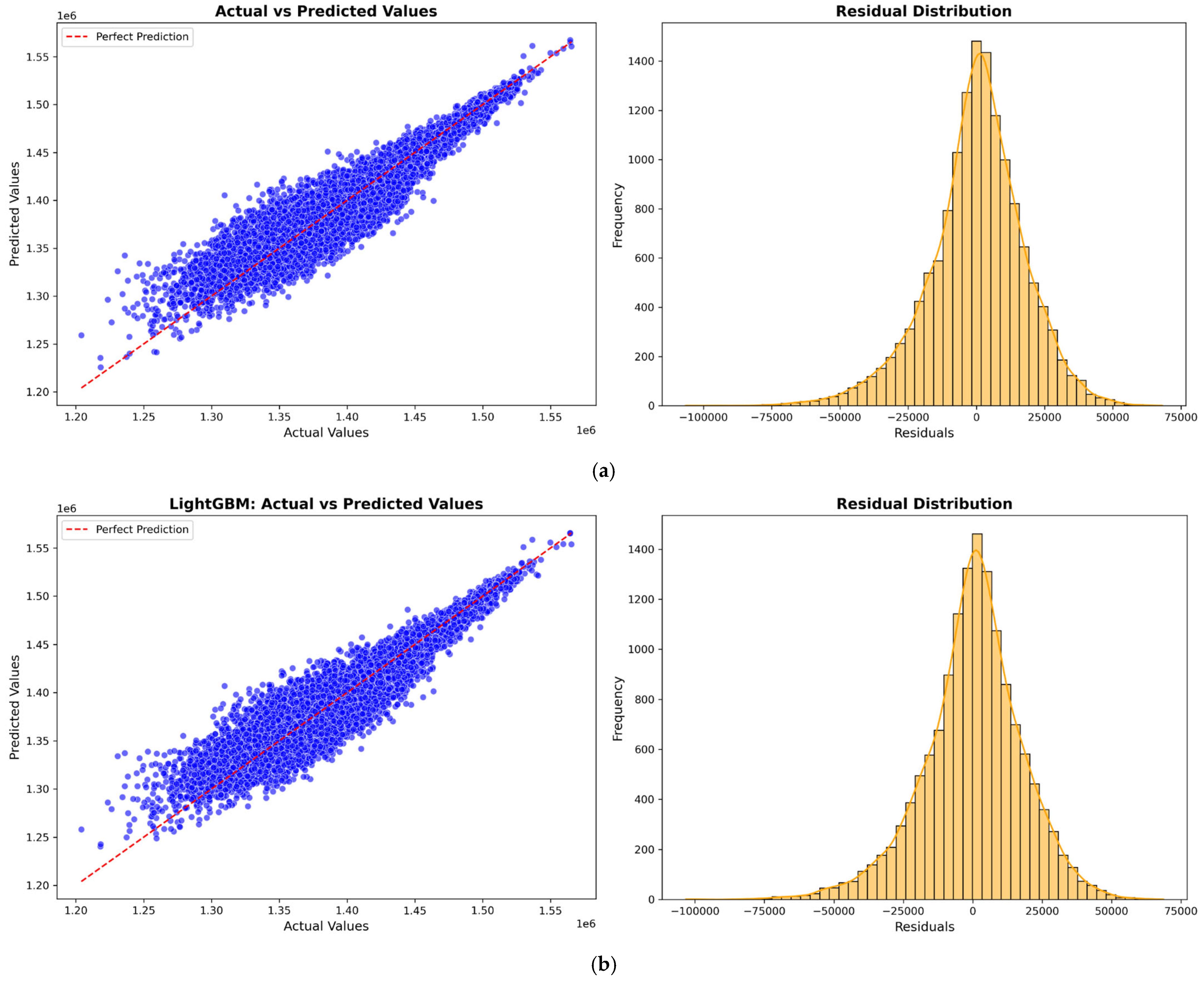
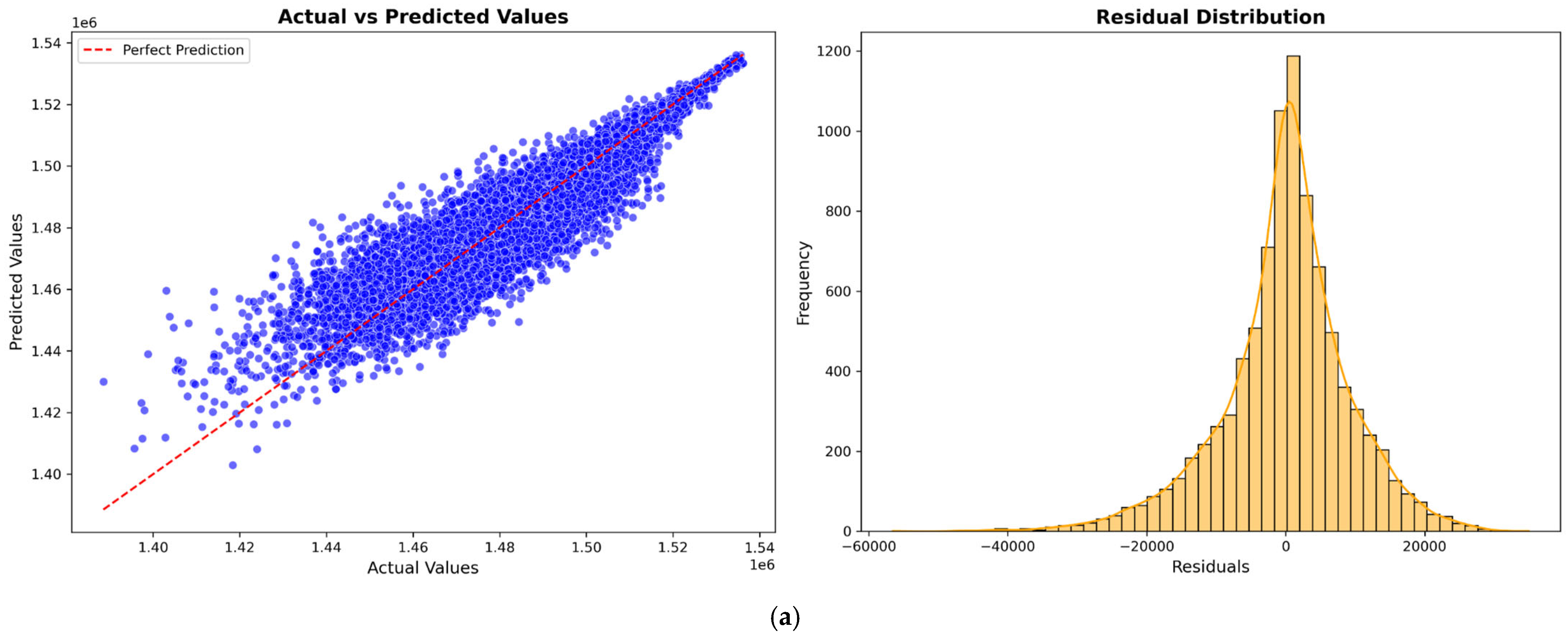
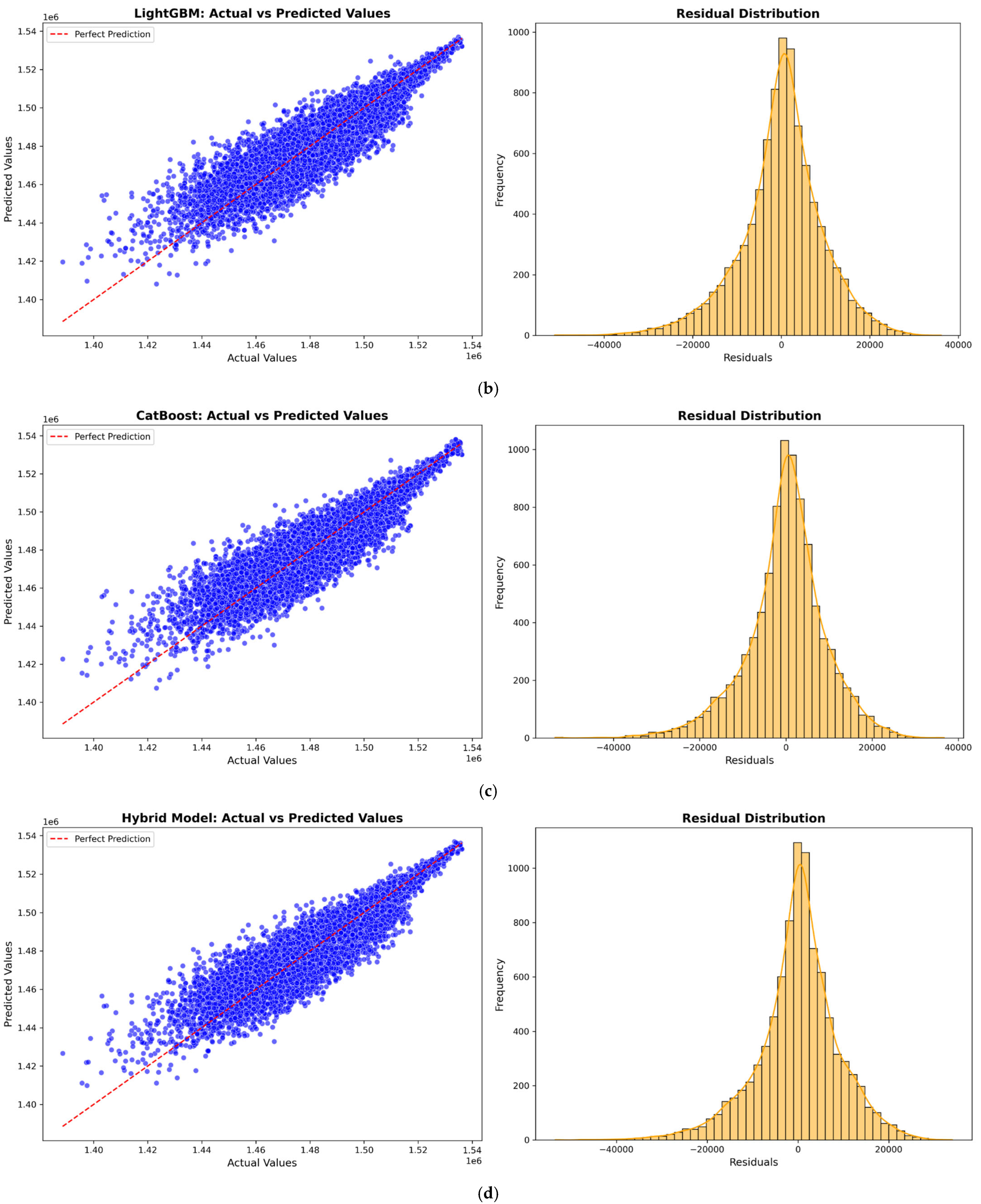
Figure 5, Figure 6, Figure 7 and Figure 8 illustrate the prediction model performance for four Australian cities (Adelaide, Perth, Sydney, and Tasmania) across four machine learning models: XGBoost, LightGBM, CatBoost, and a Hybrid model. Scatter plots show the predicted vs. actual total power output. The red dashed line represents the perfect prediction line (ideal case where predicted values exactly match actual values). The blue data points indicate model predictions. A tight clustering of points along the red line suggests better model accuracy and low residual error. Models that show less dispersion around the red line exhibit better predictive performance.

The residual distribution plot depicts the distribution of residuals (i.e., the errors between predicted and actual values). A bell-shaped error distribution centered around zero suggests that the errors are normally distributed, indicating that the model does not exhibit significant bias [46]. A narrower spread in the residuals implies lower variance and better model accuracy. It is observed that the Hybrid Model consistently improves prediction accuracy across all cities by effectively combining the strengths of XGBoost, LightGBM, and CatBoost to minimize errors.

In this study, although the dataset contains tens of thousands of instances, it remains limited in temporal diversity as it does not account for seasonal variations or long-term trends. Additionally, the dataset is specific to four Australian coastal locations (Adelaide, Perth, Sydney, and Tasmania), which means it may not accurately represent broader global wave energy patterns. Expanding the dataset to include more diverse locations and long-term observations would enhance model robustness and help reduce overfitting to local conditions. In the future, dataset coverage can be expanded to include more locations worldwide and additional WEC designs. Additionally, seasonal variations should be integrated by incorporating long-term datasets across different weather conditions.

4. Conclusions

This research successfully developed and evaluated a stacked hybrid machine learning model to predict the total power output of wave energy farms across four Australian coastal locations: Adelaide, Perth, Sydney, and Tasmania. The proposed model integrates XGBoost, LightGBM, and CatBoost as base learners, with Ridge regression as a meta-learner, leveraging ensemble learning to improve predictive accuracy and generalizability.

The stacked hybrid model consistently outperformed individual models, achieving the lowest RMSE and highest R² scores across all locations. The ensemble approach effectively reduced overfitting and improved generalization. The Sydney dataset exhibited the highest prediction accuracy (RMSE = 9089.58, R² = 0.8576) due to its relatively lower variance in wave energy output, whereas Tasmania posed the most challenging prediction task (RMSE = 45,032.37, R² = 0.8378) due to higher variability in wave conditions. Transforming spatial coordinates into Euclidean distance features and applying PCA significantly enhanced model interpretability and efficiency by reducing redundant information while retaining key predictive features. Optuna-based hyperparameter tuning and 10-fold cross-validation improved model performance by optimizing learning rates, tree depths, and regularization parameters, ensuring stable and robust predictions. Despite these advancements, limitations remain. The dataset is specific to four Australian coastal locations, limiting generalizability to other global wave energy locations. Additionally, the dataset lacks long-term seasonal variations, which may influence model predictions. In future the researchers can focus on expanding dataset coverage to include global wave energy sites and different WEC designs.