1. Introduction
The successful operation of modern gas turbines (GTs) is critical in meeting global energy demands while simultaneously reducing greenhouse gas emissions [
1]. To achieve these goals, it is necessary that GT combustors operate with high efficiency and reliability, producing low emissions. This requires a comprehensive understanding of the complex processes within combustors, such as turbulent flow, heat transfer, and mass transfer. While experimental investigations provide valuable insights, they are often limited by practical constraints and can only partially capture the intricacies of combustion processes. Therefore, numerical simulations have become an indispensable tool, offering detailed insights that complement experimental findings. However, accurately simulating GT combustion remains challenging due to its inherent complexity, necessitating the ongoing development of mathematical and numerical models to enhance predictive capabilities and validate experimental results. This work contributes to this ongoing effort and aims to advance GT technology by providing critical insights into the combustion processes within combustors.
Recent research has focused on GT combustors operating under premixed conditions, with significant Large Eddy Simulation (LES) studies on the PRECCINSTA burner demonstrating good agreement with experiments [
2,
3,
4,
5,
6,
7]. However, most simulations have overlooked partial premixing despite its link to thermo-acoustic instabilities. The TECFLAM burner [
8] has also provided valuable LES validation data with consistent results for various measurements. For non-premixed regimes, the MOLECULES combustor [
9] has been investigated, offering insights into flow-field structures under high-pressure conditions. Multi-regime burner designs [
10,
11,
12] have been investigated to produce flames with multi-regime characteristics and validate numerical models. Nonetheless, there is a lack of Detached-Eddy Simulation (DES) validation for partially premixed conditions, which pose modeling challenges due to complex turbulence–chemistry interactions. This work aims to bridge this gap by examining the DLR GT with its dual swirler design under partially premixed conditions.
A key challenge in GT combustor design is accurately modeling turbulence, especially in the presence of strong swirling flows. The DLR GT swirl injector consists of two swirler channels: the inner swirler and the outer swirler. Swirl is commonly applied to the main combustion air to create a vortex breakdown recirculation zone along the combustor’s central axis, which enhances combustion efficiency and flame stability. However, strong swirling flows introduce additional complexity into turbulence modeling due to flow curvature and pressure gradient effects that increase anisotropy [
13]. To address these challenges, this study employed DES to investigate reactive turbulent swirl flows within a GT combustor. Validation of turbulent flows, influenced by steep velocity and pressure gradients in conjunction with the combustion model, produces an independent study [
14,
15], requiring further investigation. DES utilizes the Strelets model, which combines the two-equation SST-RANS model with elements of the LES method [
16]. This approach allows the model to apply the boundary-layer coverage of SST-RANS while transitioning to LES in regions where the turbulent length scale predicted by RANS is larger than the local grid spacing. The choice of DES over LES and DNS is made to reduce computational costs. LES is expensive in boundary-layer regions because it requires a fine mesh resolution along the wall. Since the accuracy of LES depends on grid resolution, Pope [
17] recommends that the grid should resolve 80 percent of the turbulent kinetic energy away from the wall.
Simulating gas turbine combustion presents the challenge of accurately modeling the complex interaction between turbulence and chemistry. To tackle this issue, the DLR GT swirl combustor was analyzed using a partially premixed combustion model, which offers computational advantages over other models. Local mixtures (burned, unburned, or partially burned) are characterized by tracking the flame’s propagation within the partially premixed model. The model treats burnt mixtures behind the flame similarly to diffusion flames, while cold mixtures represent the unburned sections ahead of the flame front. Thermo-chemistry calculations are pre-processed, and the interaction of turbulence and chemistry is accounted for using an assumed-shape Probability Density Function (PDF). A transport equation for the progress variable (C) is utilized to track the propagation of the flame front. The results of this study can provide useful insights into the performance of partially premixed combustion models in real-world gas turbine combustion systems. Although the model has been applied to several simple combustors, relatively less attention has been paid to its performance in existing combustion systems.
The combination of these advanced numerical methods and the focus on dual swirl combustor configurations aims to extend the understanding of combustion processes, ultimately contributing to the development of more efficient, reliable, and environmentally friendly gas turbine technologies.
While large eddy simulation (LES) has been widely used to investigate combustion dynamics in swirl-stabilized flames, there is a gap in understanding the specific effects of partially premixed combustion in these configurations, particularly in terms of its impact on combustion stability, efficiency, and flow dynamics. Previous studies have primarily focused on fully premixed or non-premixed flames, but partially premixed combustion, which is more representative of real-world conditions in practical combustors, has not been thoroughly explored in this context. This study aims to address this gap by employing a partially premixed combustion model in a dual swirl combustor setup, which is not commonly found in existing LES studies. Our approach focuses on both accuracy and computational efficiency, providing insights into methane combustion behavior in industrial applications while also highlighting the potential for a robust and computationally less expensive methodology. In summary, we believe this research offers valuable contributions to the field by investigating an underexplored aspect of swirl-stabilized flames and proposing an approach with practical applications in the design and optimization of combustion systems.
2. Experimental Setup
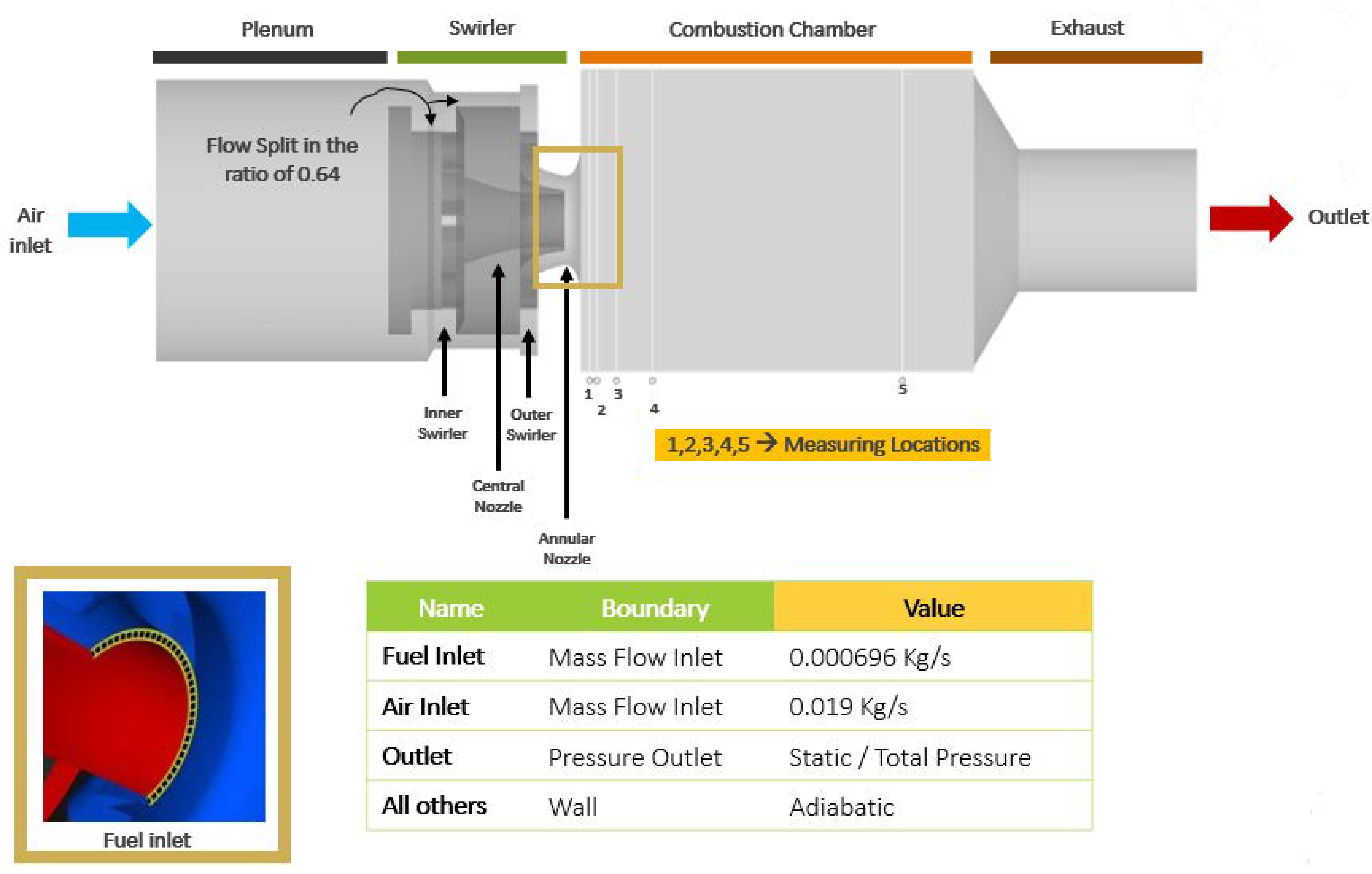
The experimental analysis was conducted by the German Aerospace Center (DLR) to investigate a dual swirl combustor that consist of a combustion chamber, a plenum, and a nozzle geometry. Dry air was supplied through an air inlet at room temperature and ambient pressure. The air was first directed through the plenum, then divided into two halves by two radial swirlers, as shown in
Figure 1. The co-swirling air was then passed into the combustion chamber through a central nozzle (
= 15 mm) and an annular nozzle (
= 17 mm,
= 25 mm, curved to an outside diameter of
= 40 mm). The diameter and height of the plenum were 79 mm and 65 mm, respectively. The central (inside) and annular (outer) nozzles had 8 and 12 radial channels, respectively, each twisted at a predetermined angle.
The fuel was introduced through a non-swirling inlet consisting of 72 square segments, each with an area of 0.5 × 0.5 mm2, positioned between the annular and central nozzles. The annular nozzle outlet and combustion chamber were positioned 4.5 mm above the central nozzle and fuel inlets. The combustion chamber was 114 mm high and had a surface area of 85 × 85 mm2. The exhaust exit diameter was 40 mm.
The air mass flow rate was maintained at 0.019 kg/s, with an inlet temperature of 330 K. Pure methane was supplied through the fuel inlet at a mass flow rate of 0.000696 kg/s and a temperature of 330 K, yielding an equivalence ratio of 0.65 for the investigated flame. The swirl number, defined as the ratio of the maximum radial velocity to the bulk axial velocity, was calculated under the assumption of perfectly guided swirler channels and conserved angular momentum within the burner. This configuration resulted in an estimated swirl number of 0.96 at the burner nozzle exit.
The mass flow rate of air was 0.019 kg/s, and the temperature at the air inlet was set to 330 K. Pure methane was introduced at a mass flow rate of 0.000696 kg/s 330 K from the fuel inlet, which resulted in an equivalence ratio of 0.65 for the current flame under examination. The swirl number is calculated as the ratio of the maximum radial speed to the bulk axial velocity, assuming that the swirler channels are perfectly guided and the angular momentum inside the burner is maintained. An estimated swirl number of 0.96 at the burner nozzle exit was obtained.
All three velocity components were measured simultaneously using Laser Doppler Anemometry (LDA) systems, and Raman scattering was employed to measure the temperature and concentration of major species. Detailed information regarding the test rig and measurements can be found in Weigand et al. and Meier et al. [
18,
19].
3. Problem Formulation
3.1. Applied Mathematics and Numerical Modeling Overview
The turbulence model employed in this study is the detached-eddy simulation (DES) model, which does not rely on a specific statistical turbulence model. While Spalart proposed a DES method based on a single-equation RANS model [
20], the present work utilizes the Strelets model [
16]. This model combines the two-equation SST-RANS model with LES elements and accounts for the boundary layer in regions where the predicted turbulent length scale (
) is greater than the local grid spacing (
). Unlike the SST model, the turbulent length scale affects the
equation’s destruction term.
The multiplier of the destruction term in Equation (
1) is defined as the
factor.
where
and
While the above approach has its benefits, it also has certain limitations, particularly in applications where flow separation in the boundary layer caused by the grid can pose challenges. When models rely on prediction of the turbulent length scale based on the local grid size, the issue of the LES mode being active in the boundary layer is a known concern. To mitigate this problem, a zonal DES limiter is proposed, which incorporates the blending function of the SST turbulence model [
21]. This technique helps to limit grid-induced separation and improve the accuracy of predictions in the boundary layer.
The model’s constants are given in Strelets et al.’s study [
16]. As compared to other physical models, like LES and DNS, the Strelets model can face challenges in accurately resolving boundary-layer flows, particularly when grid-induced flow separation occurs. Local grid size influences the transition between RANS and LES modes, potentially activating the LES mode in boundary layers where RANS would be more appropriate, leading to less accurate predictions. Dependence on the turbulent length scale and grid resolution may result in under-resolved turbulence features in complex geometries. Zonal DES limiters help mitigate grid-induced separation but can add computational complexity and require careful tuning.
The simulations were conducted using ANSYS Fluent 16.1 commercial computational fluid dynamics (CFD) software. A coupled pressure-correction scheme was employed to resolve the velocity–pressure coupling. The linear system of equations was solved using a multi-grid method, while spatial discretization utilized a second-order scheme for most variables. For species and energy equations, a bounded high-resolution scheme with second-order accuracy was applied. Transient terms were discretized using a bounded second-order implicit formulation. Parallelization in Fluent follows the Single Program, Multiple Data (SPMD) architecture, where the computational domain is partitioned into tasks executed independently across processors. Inter-process communication is handled via the Message Passing Interface (MPI). Domain partitioning and memory allocation are automated, with RAM usage evenly distributed across all CPUs. The simulations were executed on a custom-built 11-node cluster (comprising head and compute nodes) interconnected via a 1 Gb Ethernet switch. The CentOS 7.9 operating system and Rocks Cluster distribution were used for cluster management. Performance limitations arise primarily from the 1 Gb Ethernet network, which may introduce bottlenecks in MPI communication during parallel computations. While memory allocation is balanced, memory-intensive cases risk exceeding available resources, potentially limiting scalability.
3.2. Combustion Model
Partially premixed combustion is a common combustion regime in which a portion of the fuel and oxidizer are premixed before entering the combustion chamber, while the remaining fuel is injected in a non-premixed manner. In ANSYS Fluent [
22], partially premixed combustion is modeled using a mixture fraction-based approach, where a transport equation is solved for the mixture fraction (Z).
The mixture fraction is defined as the mass fraction of fuel in the combustion mixture and is expressed as follows:
where
is the density of fuel and
is the density of the mixture. The transport equation for the mixture fraction is expressed as follows:
where
is the velocity vector,
is the diffusivity of the mixture fraction, and
is the mass injection rate of fuel. The mixture fraction is used to compute the local fuel–air equivalence ratio, a key parameter in the combustion process. The relationship between the mixture density and the mixture fraction is given by the following formula:
where
is the density of the oxidizer [
23].
The partially premixed combustion model in ANSYS Fluent also includes a transport equation for the progress variable (
c), a scalar quantity representing the local extent of the combustion process. The transport equation for the progress variable is expressed as follows:
where
is the diffusivity of the progress variable and
is the source term due to chemical reactions. The progress variable is used to track the location of the flame front, which separates the unburned reactants from the burned products.
To account for the effects of turbulence on the combustion process, ANSYS Fluent uses the Turbulent Flame Speed Closure (TFC) model, which relates the mean turbulent flame speed (
) to the local turbulence intensity and length scales. The mean turbulent flame speed is expressed as follows:
where
is the turbulent diffusivity of the mixture fraction,
is the molecular diffusivity of the mixture, and
is the laminar flame speed. The TFC model allows for the influences of both turbulence and chemical kinetics on the combustion process.
In this study, the temperature and other thermodynamic properties are derived based on the mixture fraction (Z) and progress variable (C) using the partially premixed combustion model. The energy equation is not solved separately; instead, the temperature field is obtained from the combustion model, which utilizes chemical equilibrium tables to determine the thermodynamic state of the fluid. This approach effectively captures heat transfer and thermal dynamics through the interactions of (Z) and (C). The partially premixed combustion model in ANSYS Fluent uses a mixture fraction-based approach to model fuel–air mixing and includes transport equations for the mixture fraction and progress variable to track the combustion process. The turbulent flame speed closure model is used to account for the effects of turbulence on the combustion process.
The partially premixed combustion model is computationally less expensive, but it has limitations as compared to detailed chemical kinetics modeling. The mixture fraction-based approach assumes an equilibrium state or near-equilibrium condition, which may not capture transient or local non-equilibrium phenomena accurately. Simplifications in modeling the progress variable can fail to fully represent detailed chemical kinetics, particularly in highly reactive or non-premixed zones. The assumption of a predefined laminar flame speed () limits the ability to capture varying flame characteristics under different operating conditions. The TFC model relies on empirical correlations for turbulent diffusivity and flame speed, which may not be accurate for all turbulence and flame interaction regimes. Using precomputed equilibrium tables for thermodynamic properties limits flexibility in simulating cases with significant deviations from equilibrium.
3.3. Mesh Generation
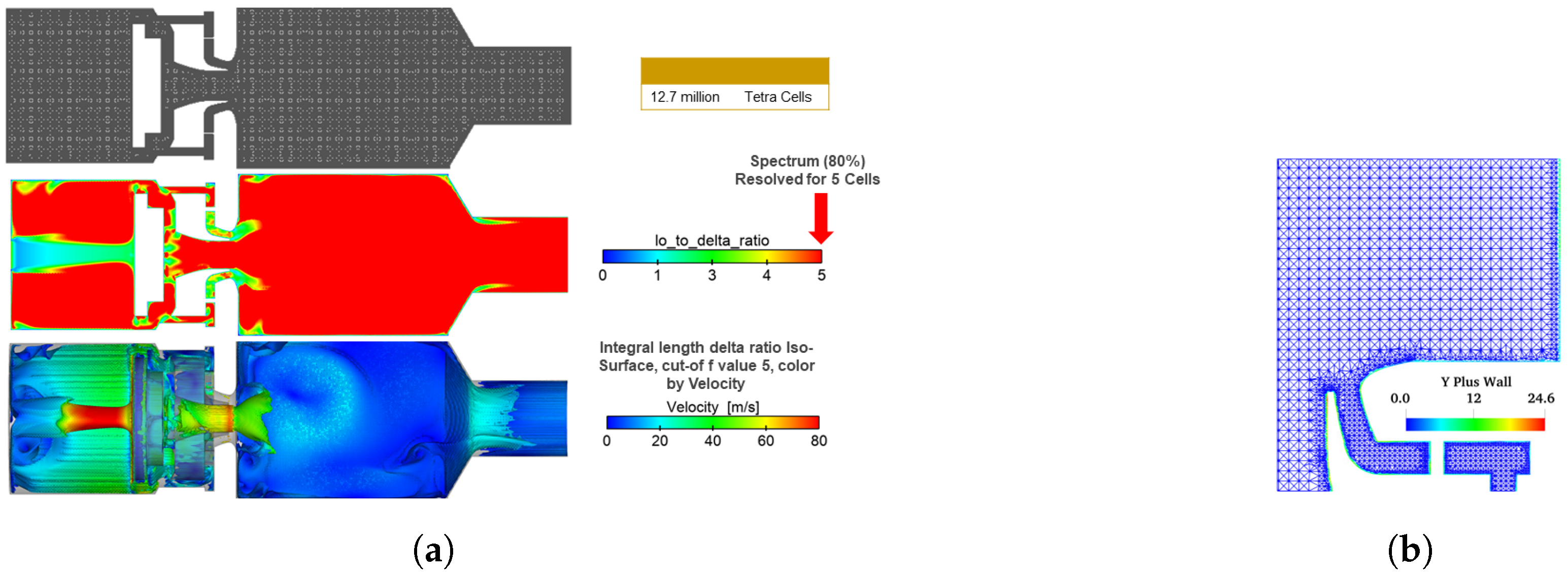
The mesh resolution is a critical aspect of the computational setup, as it is essential to ensure that the simulation captures the relevant physical phenomena. In this study, the mesh resolution is determined based on the ratio of the integral length scale to the size of the grid cells (). The integral length scale measures the size of the most significant turbulent structures in the flow and is calculated as the ratio of the kinetic energy (k) to the rate of dissipation (). The K-omega SST model is used to obtain values for the kinetic energy and dissipation rate, which are then used to calculate the integral length scale.
The integral length scale must be resolved within a few grid cells in each direction to ensure proper mesh resolution. A general guideline is to resolve at least 80% of the turbulent kinetic energy by capturing eddies with sizes larger than half the integral length scale. The mesh statistics are represented in
Figure 2a, which shows a contour plot of the ratio of the integral length scale to the delta. The plot indicates the mesh resolution level, with higher values represents a well-resolved mesh. A maximum capture value of 5 or higher on the plot represents the cumulative turbulent kinetic energy against the length scale of eddies based on Kolmogorov’s energy spectrum.
In this study, the mesh resolution was selected to ensure that the integral length scale is adequately resolved and that the turbulent kinetic energy is captured to a satisfactory level. The maximum value of (
) along the combustion chamber wall is 24.6, as shown in
Figure 2b, which is considered appropriate for this kind of simulation where shear flows dominate inside the combustion chamber.
3.4. Boundary Conditions
The numerical boundary conditions are illustrated in
Figure 1. Air enters through the air inlet with a mass flow rate of 0.0176 kg/s and a temperature of 330 K. Pure methane is introduced from the fuel inlet at a mass flow rate of 0.000696 kg/s and a temperature of 330 K. The turbulent intensity at the air and fuel inlets is set to 5% (medium) and 15% (maximum), respectively. The eddy length scale at both inlets is 0.0005 m.
The wall boundary condition at the combustion chamber wall is set to 1050 K, while the bottom wall boundary condition is set to 600 K. All other wall boundary surfaces are assumed to be adiabatic.
4. Results and Discussions
4.1. Numerical Measurements of Mean Values and RMS Fluctuations
The reported results are based on time-averaged data collected after the combustion initialization process. The averaging process spans four residence times, with quantitative analysis performed after two residence times to ensure stability in the results.
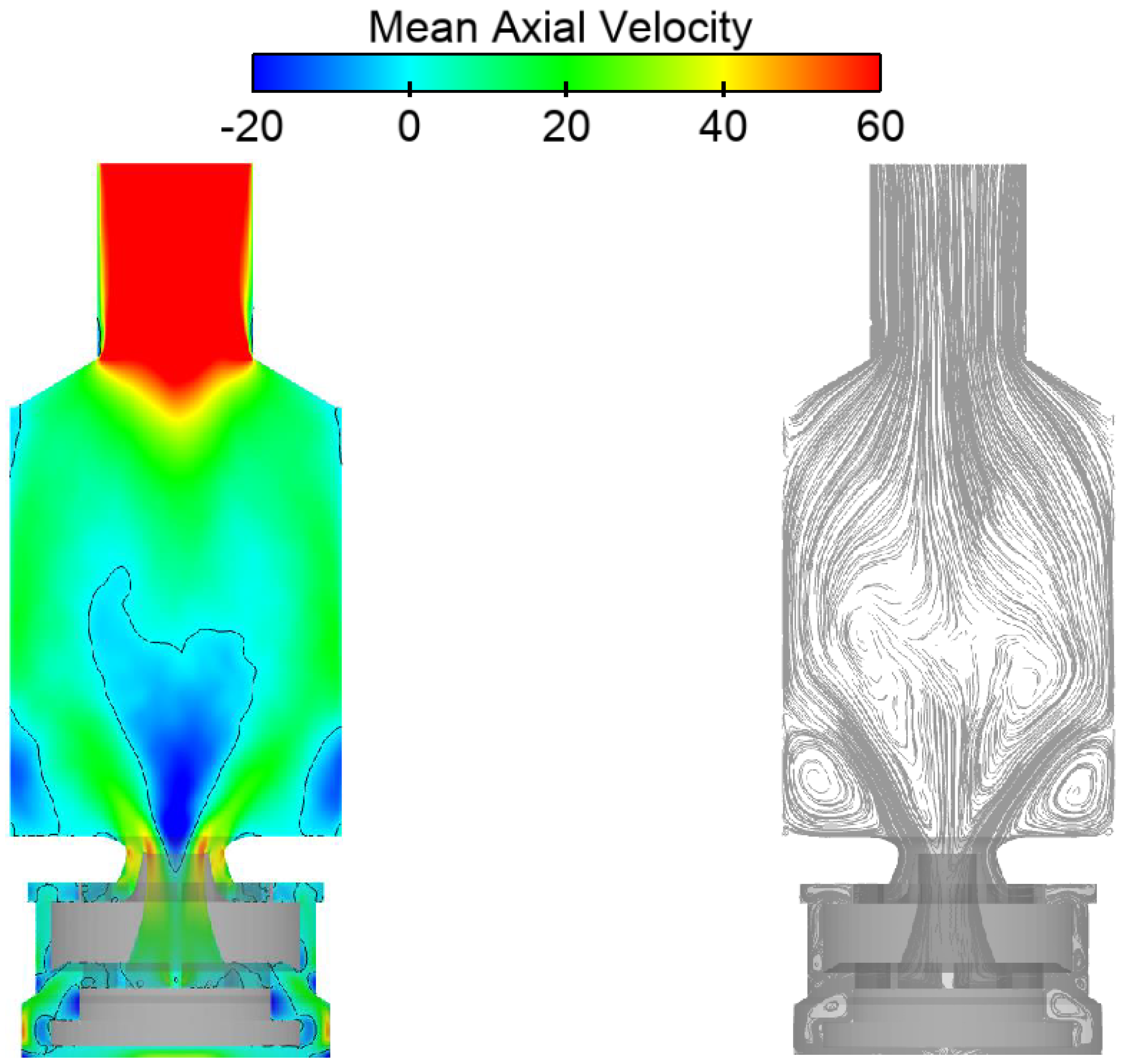
Figure 3 depicts the time-averaged axial velocity field within the combustor, stabilized by enclosed swirl burners with concentric inflow. The two-dimensional contour plot and superimposed streamlines reveal the complex flow structure, characterized by distinct Internal and Outer Recirculation Zones (IRZ and ORZ, respectively) adjacent to the combustion chamber walls. Despite the square geometry of the chamber, the flow field retains approximately axial symmetry, though minor discrepancies between experimental and numerical results are evident. Both the IRZ and ORZ exhibit high turbulence levels, with periodic fluctuations in size and position over time. The region between these zones corresponds to the fresh gas inflow, acting as the primary pathway for unburned reactants. The figure underscores the dynamic nature of the flow, illustrating how recirculation zones govern flame stabilization and mixing processes. While the numerical model captures the overall flow topology, deviations in symmetry and turbulence dynamics highlight challenges in replicating experimental conditions.
Figure 3 depicts a contour plot of the time-averaged axial velocity and corresponding streamlines. The solid black line marks the zero-axial-velocity contour, delineating the boundaries of the recirculation zones. Negative axial velocities at the center indicate the internal recirculation zone (IRZ) generated by vortex breakdown. The IRZ spans approximately 60 mm in length and 40 mm in width, extending roughly 4 mm into the combustor’s primary and central air nozzles in the time-averaged flow field. Adjacent to the combustion-chamber corners, the outer recirculation zone (ORZ) forms, separated from the IRZ and the fresh inflow stream by shear layers. The IRZ exhibits high-velocity gradients and temporal fluctuations, rendering it dynamically unstable, with a time-dependent position and dimensions. A small recirculation bubble is also observed near the diffuser exit. The time-averaged flow separates approximately 2.5 mm below the burner mouth; however, due to flow unsteadiness and the absence of a sharp separation edge, this point fluctuates along the wall. Despite the combustion chamber’s square geometry, the flow field retains approximately axial symmetry. Minor deviations from symmetry are evident in both experimental and numerical results, underscoring the challenges in replicating turbulent flow dynamics.
The air mass flow in the combustion chamber is split into two streams by passing through the swirlers in a fixed ratio of 0.64, which is not influenced by the choice of turbulence model. The division of the air mass flow rate is determined by the relative flow rate of air passing through the central (inner) swirler and that passing through the annular (outer) swirler. This fixed ratio ensures a stable and predictable combustion process, regardless of the turbulence level in the flow.
4.1.1. Comparison of Mean Velocity Profiles with Experimental and Other Numerical Models
Figure 4,
Figure 5 and
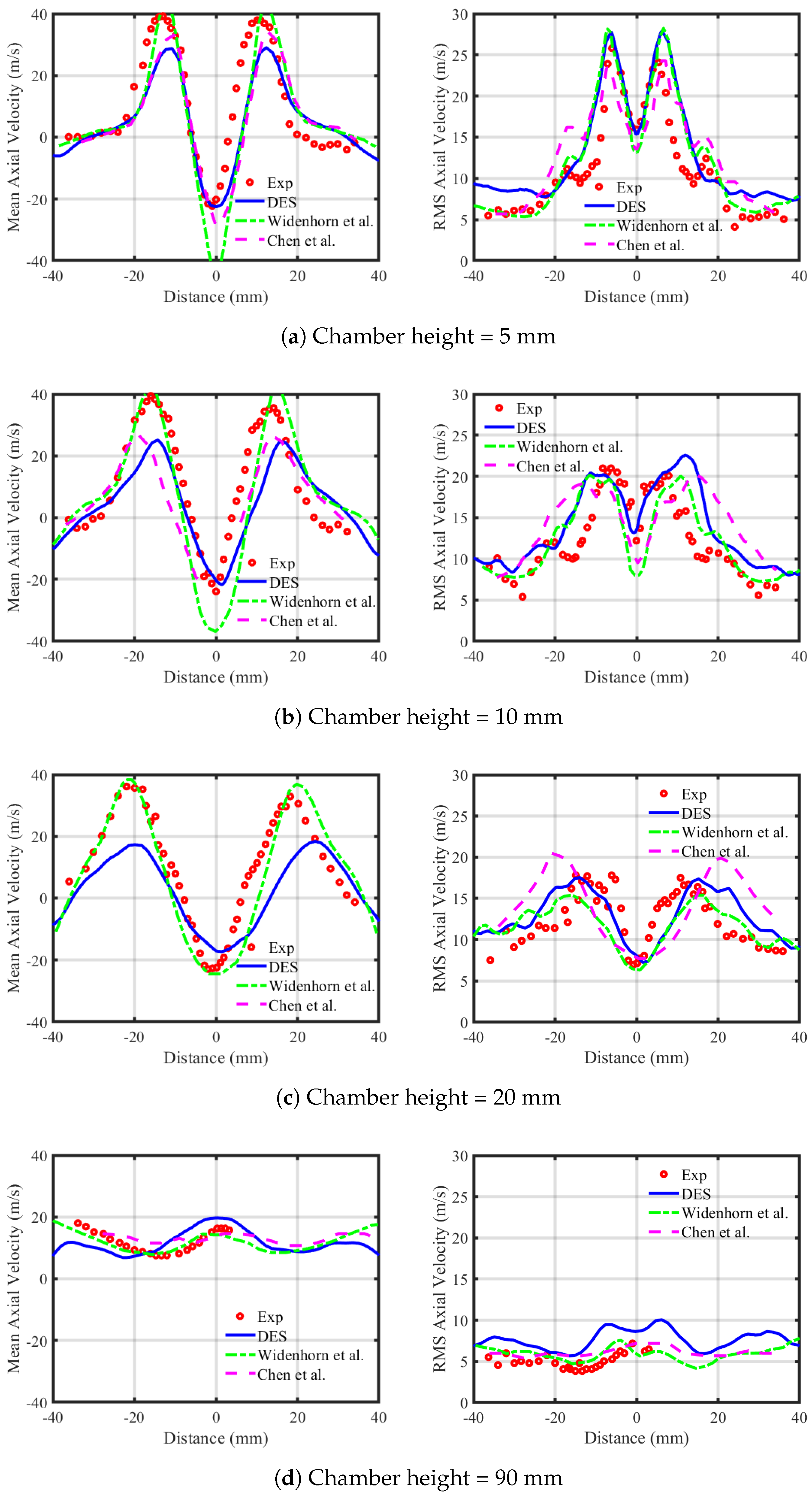
Figure 6 present numerical results for the time-averaged and root mean square (RMS) velocity profiles in the axial, radial, and tangential directions, respectively. These are compared with experimental data at multiple heights within the combustion chamber to evaluate the accuracy of the numerical simulations. Each figure is divided into two parts: the first half displays the mean velocity profiles, while the second half illustrates the corresponding RMS fluctuations. In the mean velocity profiles of
Figure 4 (axial direction), a positive peak velocity of approximately 30 m/s is observed at a height of 5 mm, corresponding to the incoming fresh gas stream. For the radial component (
Figure 5), inwardly directed velocities in the region of
Y > 16 mm signify the outer recirculation zone (ORZ), with maximum radial velocities reaching roughly half the magnitude of the axial component. The tangential velocity profiles (
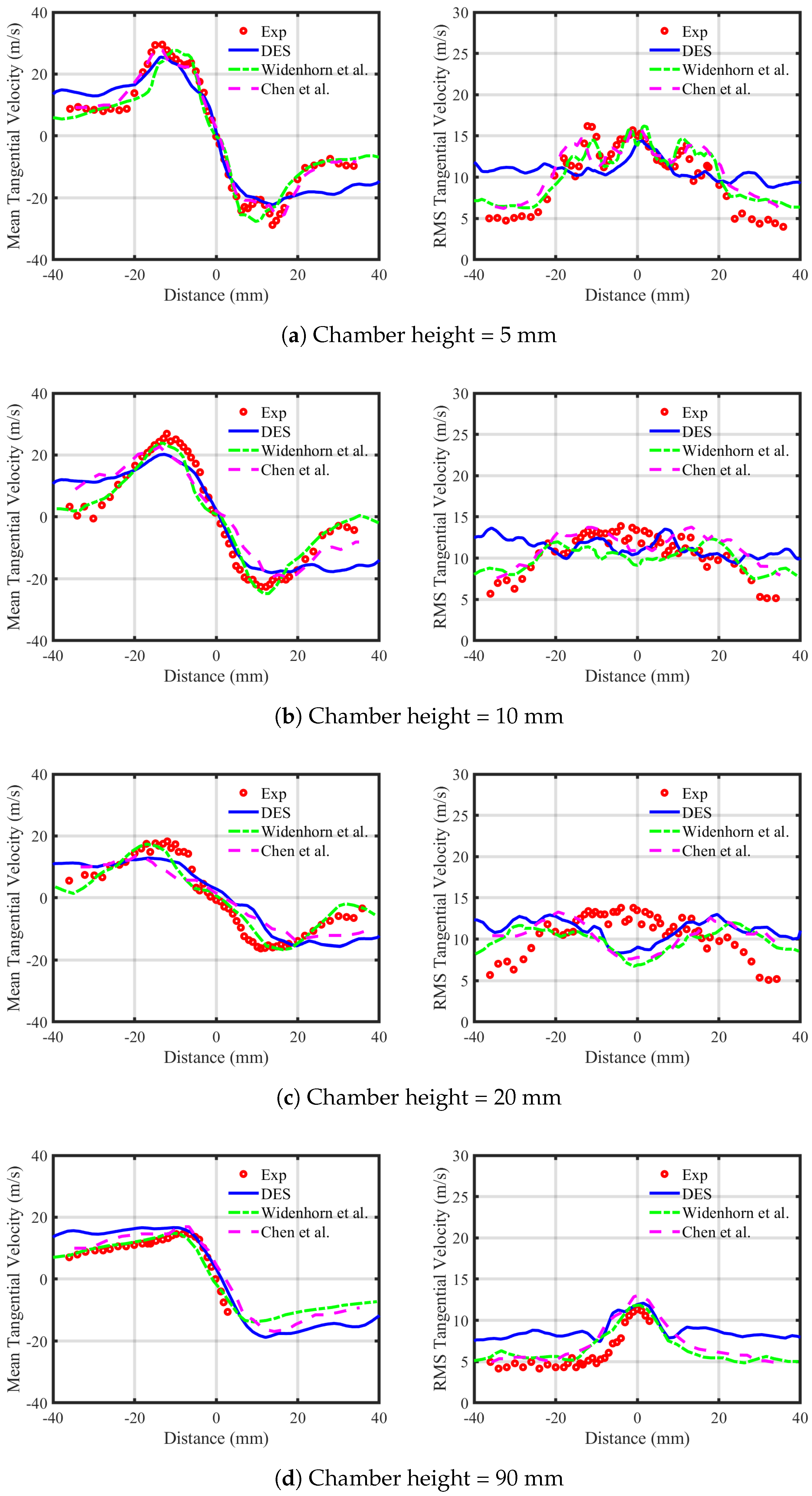
Figure 6) show relatively constant values within the ORZ, where maxima reflect contributions from the central and annular nozzle flows. However, the simulations fail to capture the minimum tangential velocity induced by the fuel nozzle and its wake in the ORZ in the range of 5 mm ≤ Y ≤ 20 mm.
Similarly, these results are compared with reference numerical data from the studies conducted by Widenhorn et al. [
14] and Chen et al. [
24]. Widenhorn et al. [
14] implemented the Scale-Adaptive Simulation (SAS) method to simulate the flow, while Chen et al. used large eddy simulation (LES). In comparison to these reference numerical results, the present mean axial velocity profiles come much closer to predicting the axial velocity than those reported in the study by Chen et al. [
24]. Widenhorn et al. [
25] predicted significantly higher peak values for both the lower and upper peaks. This numerical pattern remains consistent across all mean axial velocity profiles from a height of 5 mm to 90 mm. The mean radial velocity profiles are more accurate compared to the experimental results. In comparison to the present study, the radial velocity exhibits a similar profile but is lower in magnitude near the injector at
mm when compared to that reported in the study by Chen et al. [
24]. At a height of 20 mm, Chen et al. [
24] predicted higher peak values of mean radial velocity compared to both Widenhorn et al. [
25] and the present study. The mean tangential velocity profiles reported by Chen et al. [
24] align more accurately with the experimental results, while the models proposed in the study by Widenhorn et al. [
25] and in the present study also closely follow the experimental trends.
4.1.2. Comparison of RMS Velocity Profiles with Experimental Data and Other Numerical Models
The second panels of
Figure 4,
Figure 5 and
Figure 6 display the root mean square (RMS) profiles of the axial, radial, and tangential velocity components, respectively. The axial-velocity RMS profiles exhibit maximum fluctuations in the shear layers between the incoming fresh gas and the internal recirculation zone (IRZ), with peak values of 28
/
5
from the nozzle. These RMS values indicate that the IRZ is dynamically unstable, fluctuating predominantly in the axial direction, while the outer recirculation zone (ORZ) varies radially. At a height of 10
, the flow characteristics resemble those observed at 5
. However, at 20
, the RMS values align with measurements at the nozzle exit, albeit with a slight overestimation of the strength of the recirculation zone. The numerical results agree with experimental data for time-averaged axial velocity profiles, though turbulent peak values at 5
are marginally underestimated. For the radial velocity component, the maximum RMS values occur in the shear layers between the fresh gas inflow and the ORZ (
). Broad peaks in turbulent fluctuations near
(axial direction) highlight shear-layer instabilities. While radial-velocity RMS profiles at the center line are accurately predicted at
and
, discrepancies in peak magnitudes persist. Notably, results at
and
show excellent agreement with experiments. The tangential-velocity RMS profiles prove more challenging to predict compared to axial and radial components. Accuracy is particularly reduced in the ORZ, whereas the IRZ exhibits strong agreement with experimental data across all measurement positions. This contrast underscores the limitations of the numerical model in resolving tangential dynamics within complex recirculation zones. The summary of peak values of numerical mean and RMS velocity components, in comparison with experimental values, is presented in
Table 1.
The turbulent velocity fluctuations across axial, radial, and tangential components are summarized in the accompanying figures. These results highlight that the axial velocity component exhibits a maximum RMS value of approximately 26 / within the shear layers of the incoming fresh gas stream, located between the outer and internal recirculation zones (ORZ and IRZ, respectively). The radial component follows a comparable trend, with peak RMS values observed in both the fresh gas stream and ORZ. Elevated RMS levels in the shear layers near the air and fuel inlets suggest intense mixing dynamics. A sharp gradient in axial velocity fluctuations near the air–fuel nozzle implies instability in the local shear layers, challenging the assumption of a stable IRZ structure. While IRZ fluctuations predominantly occur in the axial direction, ORZ variations are concentrated radially. Turbulent activity diminishes toward the chamber center, contrasting with the highly dynamic behavior near the fresh gas inflow. At a height of 20 , axial and radial turbulence intensities decrease significantly, with flow characteristics remaining nearly consistent between 5 and 10 . By 90 , all three velocity components display uniform behavior, marked by minor RMS peaks at the rotational axis and chamber walls. These peaks likely arise from vortical structures (e.g., tornado-like flows) influencing the velocity field.
In comparison with the reference numerical results, the axial-velocity RMS profiles show some differences. At a height of 5 mm, Chen et al. [
24] predicted lower peaks of axial-velocity RMS compared to Widenhorn et al. [
25] and the present study. However, in comparison with the experimental results, all numerical results exhibit similar trends. At a height of 10 mm, the present study predicted lower values in the inner recirculation zone (IRZ) but higher peak values while still following a trend similar to that of the reference numerical results when compared to experimental data. At a height of 20 mm, Chen et al. [
24] predicted higher peak values compared to the present work and other numerical studies. At a height of 90 mm, the present study predicted higher values than the reference numerical results. For the radial RMS profiles, the present study accurately captured the inner peaks of radial RMS at a height of 5 mm, whereas the reference numerical results overestimated these peaks. At a height of 10 mm, both Chen et al. [
24] and the present study captured the IRZ or inner shear-layer fluctuations more accurately compared to Widenhorn et al. [
25]. The remaining radial RMS profiles show similar trends. The tangential RMS profiles exhibit some fluctuations when compared with the reference numerical results but generally follow a trend similar to that of the experimental data.
4.2. Instantaneous Flow Structures
The time-averaged results only provide a general overview of the flow characteristics within the combustion chamber and do not capture the unsteady flow structures that are crucial to understanding the combustion process.
Figure 7 shows the dominant unsteady flow structures in the chamber, characterized by a V-shaped incoming fresh stream of swirl gas. The surface also restricts streamlines in relationship with contour plots of instantaneous axial velocity, indicating the presence of small-scale, unstable vortices close to the inner and outer shear layers. These small structures, along with the high turbulent intensity between the shear layers, are vital in promoting the intense mixing of cold fresh gas and hot burning gases recirculating from the IRZ and ORZ, which aids in stabilizing the flame and contributing to the ignition process of fresh gases. The recirculation zone comprises small recirculation pockets represented by solid black lines rather than one large IRZ, as shown in
Figure 3.
The highlighted vortices and the undulated inner shear layer are spatially offset, forming a staggered zig-zag pattern that widens with increasing distance from the center line toward the nozzle. This configuration suggests the presence of a Precessing Vortex Core (PVC), a hydrodynamic instability prevalent in both non-reacting and reacting flows at elevated swirl numbers. The precession frequency and amplitude depend critically on the swirl number, axial confinement, and boundary conditions. The time-averaged flow field inadequately resolves the zig-zag vortices and their helical trajectories. Furthermore, the helical structure dynamically shifts position over time, rendering steady-state simulations ineffective for accurate prediction. The PVC phenomenon involves the vortex core precessing around a mean axis while maintaining a helical shape, a behavior that profoundly influences combustion stability and emissions.
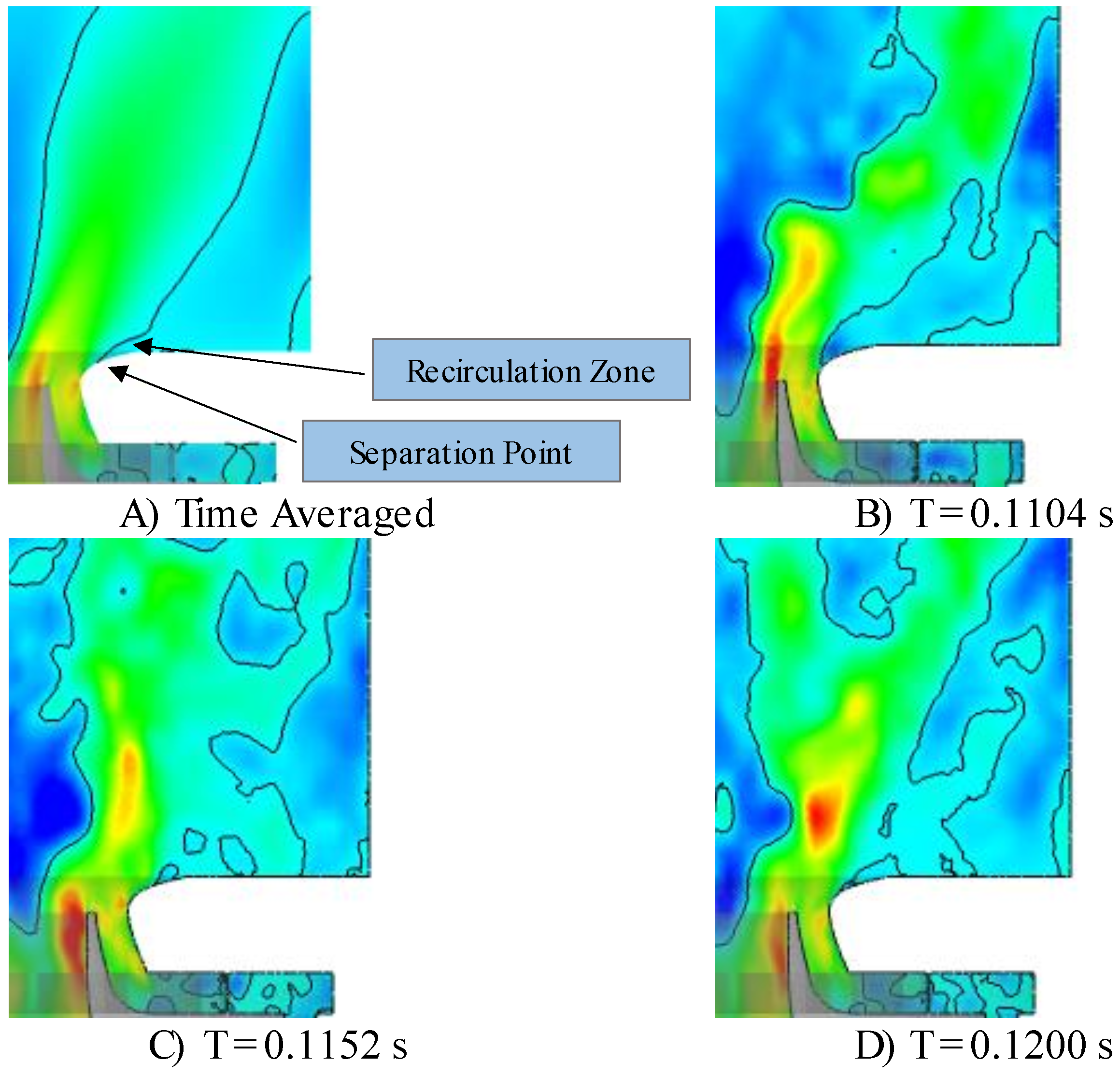
Figure 8A provides information on the time-averaged axial velocity and recirculation zones, showing a small recirculation bubble on the contour of the annular nozzle due to the unstable flow separation at the wall. A sharp edge does not cause this separation, as the flow is highly unstable in nature. However, the separation point fluctuates along the wall, as shown in
Figure 8B–D. The size and shape of the ORZ are heavily dependent on time, and small vortices are generated during the separation and subsequently combine to form the ORZ.
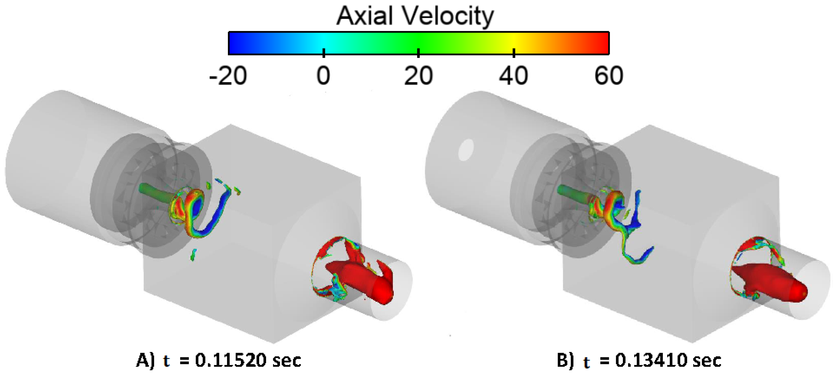
Figure 9 represents the continuous evolution of the PVC on different pressure iso-surfaces, colored according to axial velocity. Increasing the pressure causes the PVC to evolve and makes a smaller structure visible.
4.2.1. Precessing Vortex Core
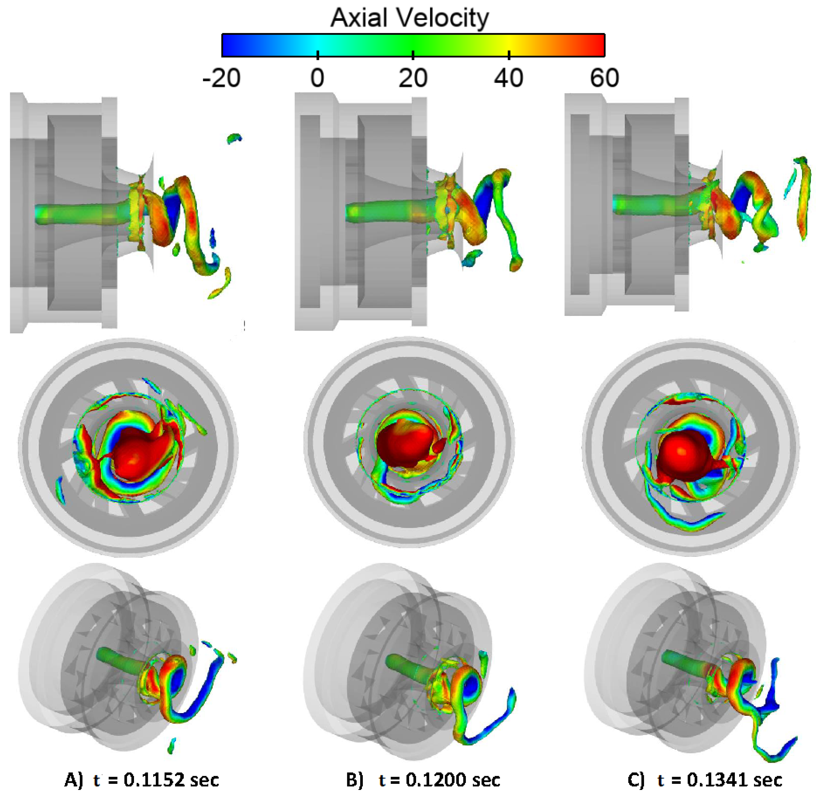
The precessing vortex core (PVC) is a complex, irregular flow structure that rotates around the central axis and significantly influences combustion dynamics. Its formation and behavior depend on parameters such as the swirl number, equivalence ratio, and combustor geometry, as extensively analyzed by Syred et al. [
26]. Numerical simulations conducted by Widenhorn et al. [
14,
25,
27] confirm the presence of PVC across multiple load conditions in the current combustor design.
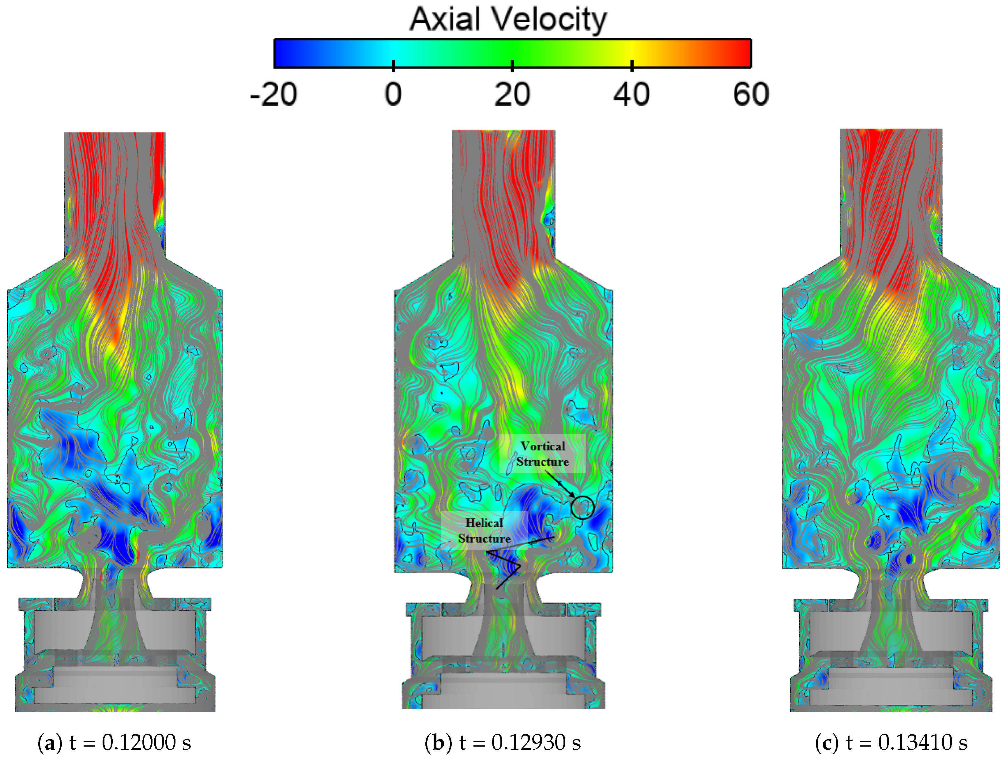
Figure 10 visualizes the PVC using low-pressure iso-surfaces color-mapped according to axial velocity to capture its transient evolution. These iso-surfaces are shown at three distinct time instances, highlighting the intricate and unsteady nature of the PVC.
4.2.2. Vortical Structure
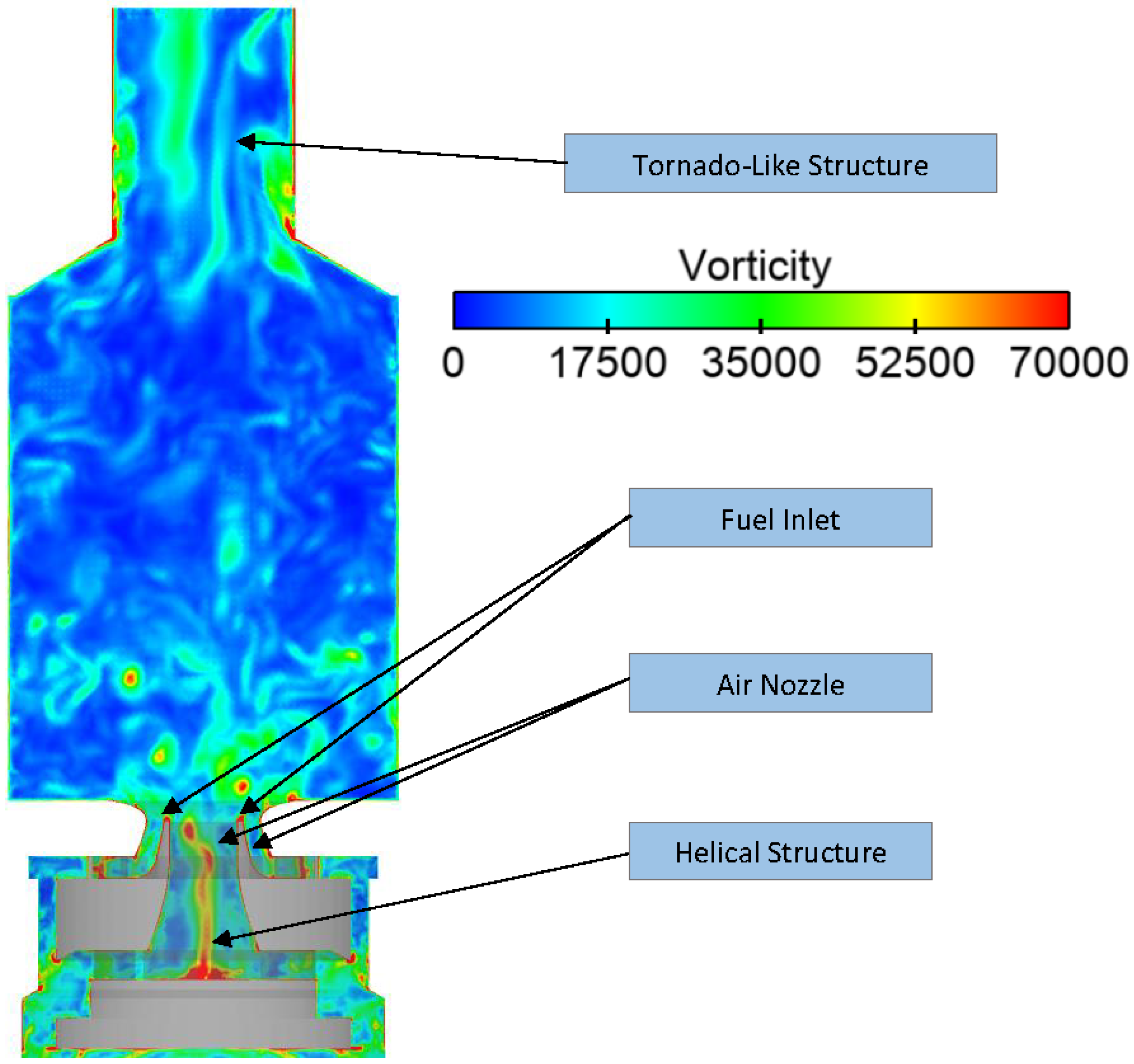
Figure 11 depicts a vortical structure in the upper combustion chamber, where an unsteady vortex core resides in the exhaust pipe. This tornado-like structure, experimentally investigated by Stopper et al. [
28], arises from the combustion chamber’s rapid radial contraction, which amplifies the swirling flow’s angular velocity. The resulting precessing vortex core (PVC) migrates into the combustion chamber, altering the time-averaged shape of the inner recirculation zone (IRZ) and influencing the transport of recirculated gas to the combustor nozzle. As a common feature of swirling flows, the PVC precesses around its axis and interacts dynamically with other flow structures, including the IRZ and outer recirculation zone (ORZ). The PVC’s significance in combustion systems stems from its ability to enhance turbulent mixing and stabilize combustion. By inducing strong axial and radial flow oscillations, the PVC improves fuel–air mixing, accelerates flame speed, and modifies time-averaged flow patterns, thereby reducing emissions and promoting combustion stability. Experimental studies highlight that PVC characteristics—such as size, precession frequency, and stability—are governed by parameters like the swirl number, combustor geometry, and operating conditions. For instance, higher swirl numbers intensify tangential momentum, directly affecting the PVC’s evolution and interaction with recirculation zones.
4.2.3. Vorticity
To clarify, there are four distinct reasons for the occurrence of vorticity in the combustion chamber. The first reason is the interaction of the helical structure with the inner shear layer, as previously mentioned. The second reason is the precessing vortex core (PVC), which rotates around the central axis of the combustion chamber, as shown in
Figure 12. The third reason is the vortex breakdown phenomenon, which is depicted in a spiral shape as it approaches a stagnation point due to the geometric change between the fuel inlet and the conical part of the air nozzle at the combustion chamber entrance. This geometric change causes a sudden swirl increase, generating vorticity. The fourth reason is the occurrence of a vortical structure in the upper part of the chamber, as depicted in the figure. Vorticity can also occur due to a vortex core in the exhaust pipe.
4.3. Temperature Field, Heat Release, and Mass Fractions
4.3.1. Time-Averaged Temperature Profiles
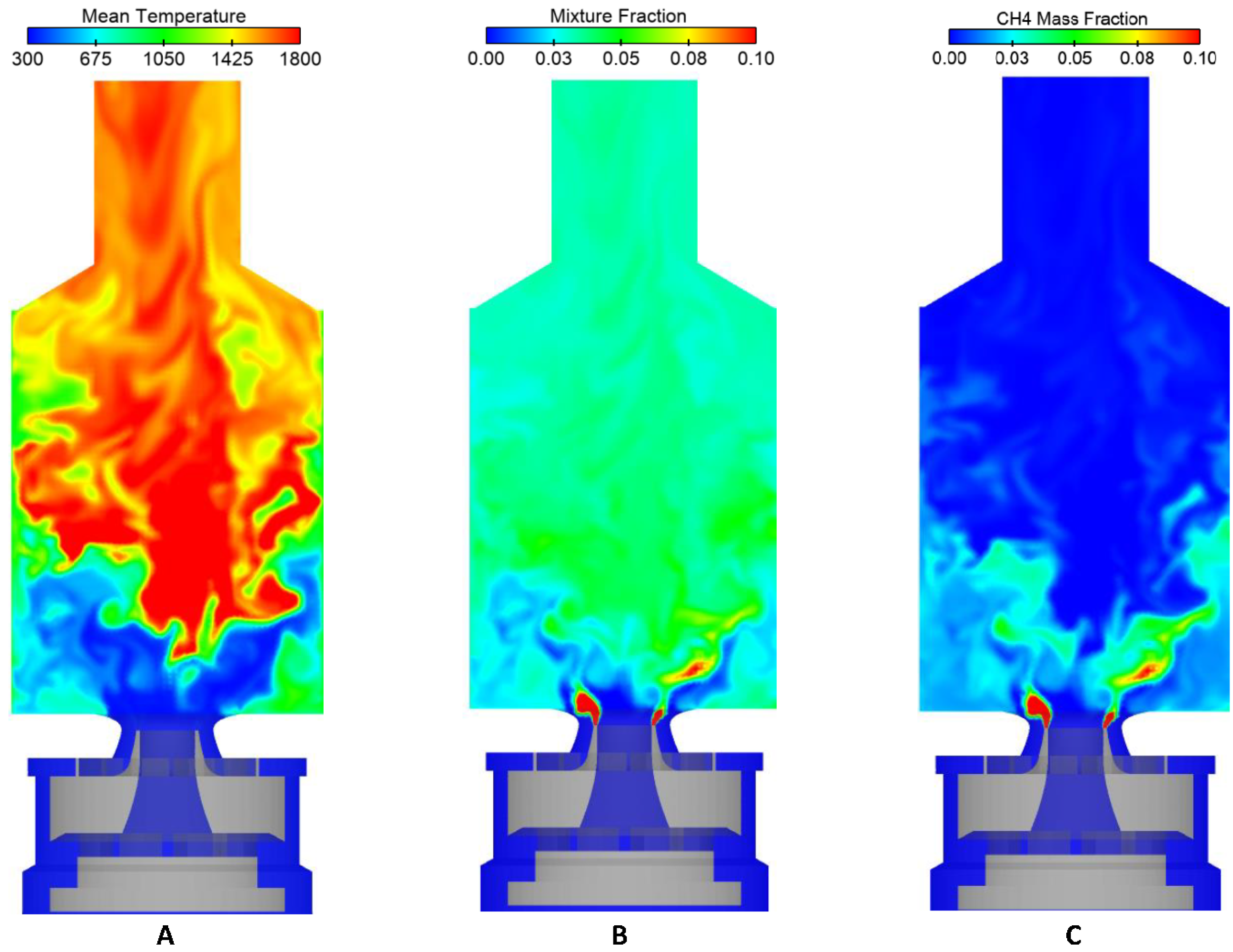
The temperature distribution in the combustion chamber is a critical parameter in understanding the combustion process. As shown in
Figure 13A, the flame takes on a conical shape, a common characteristic of many combustion systems. The mean temperature is highest near the nozzle exit, gradually decreasing as it moves toward the combustor walls. The time-averaged flame root, which is the point where the flame is anchored to the nozzle exit, is approximately 15 mm above the nozzle exit. This position indicates that the flame is partially premixed before ignition, meaning that the fuel and air are partially mixed before combustion. The swirl motion of the air and fuel in the combustion chamber generates this partial mixing. The partially premixed flame structure is beneficial for reducing emissions and improving combustion efficiency, as it allows for more uniform mixing and better control of the combustion process.
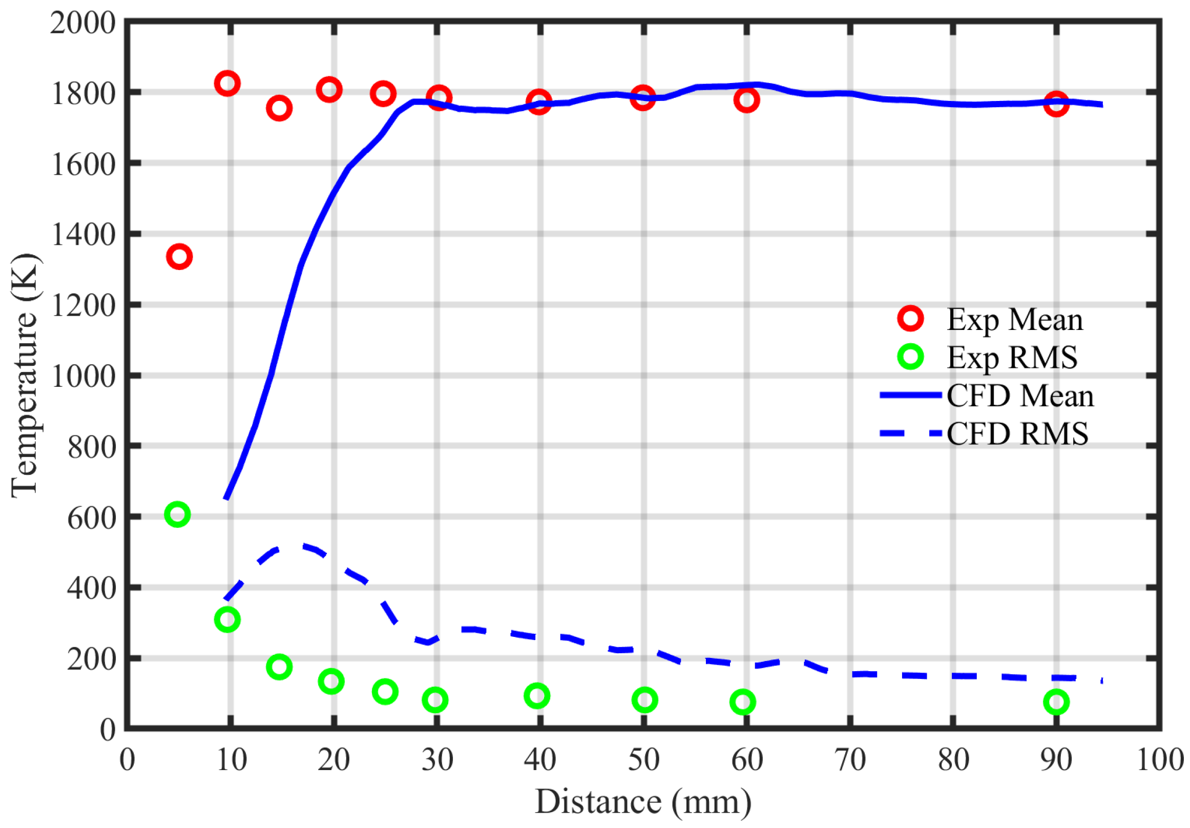
The comparison of numerical and experimental time-averaged temperature profiles, shown in
Figure 14, provides valuable insights into the simulation’s accuracy and the flame’s behavior. The distribution of mean temperatures reveals that the flame exhibits a conical shape, consistent with many combustion processes. At a height of 15 mm, corresponding to the flame root or anchoring point, the numerical center-line temperature is approximately 1800 K, which is recognized as a main combustion region. However, a significant discrepancy at a height of 10 mm in the combustion chamber is observed between the numerical and experimental data in the regions of the high-shear layer. The lowest simulated mean temperature is 600 K, which may indicate limitations in the simulation or measurement technique.
The turbulent fluctuations, quantified by the root-mean-square (RMS) temperature, are also compared between the numerical and experimental data. The results show that the turbulence intensity is higher in the numerical simulation than in the experiment, suggesting that the simulation may overpredict the turbulent mixing in the combustion chamber. Nonetheless, the comparison indicates a good agreement between the numerical and experimental data in the regions of low temperature, which are attributed to the approaching fresh gas stream.
The distribution of the time-averaged temperature provides valuable information about the combustion process and reveals the effects of mixing and heat transfer on the flame structure.
Figure 14 shows that, for y > 10 mm, the mean temperature increases with height, primarily due to the mixing of the hot exhaust gas from the ORZ with the unburned gas. At h = 25 mm, the maximum mean temperature is achieved, indicating the location of the flame’s peak temperature.
Within the IRZ, the maximum time-averaged mean temperature is T = 1827.6 K, which closely matches the experimental value of T = 1827 K. This region’s mixing fraction (f) is higher than the global value, indicating that the IRZ is well-mixed and has a higher concentration of reactants. On the other hand, the ORZ has a lower temperature level compared to the IRZ. This can be attributed to the leaner mixture and heat losses to the ORZ wall.
The numerical results also capture the temperature gradients across the flame structure, with the highest temperatures occurring near the flame root and decreasing towards the flame tip. In addition, the turbulent fluctuations (RMS) of the temperature exhibit high values in the regions of the shear layers, where the mixing of the reactants and products is most intense. Overall, the numerical temperature profiles agree well with the experimental data and provide insights into the complex flame dynamics in the combustion chamber.
The time-averaged temperature profiles obtained through simulation are in good agreement with the experimental results, except for a slight deviation observed at a height of 5 mm, where the temperature near the center line is underestimated. The turbulent temperature fluctuation profiles obtained through simulation also agree with the experimental profiles, with peak values and overall shape closely resembling the measured data. However, at a height of 5 mm, the simulated turbulent temperature changes at the center line are slightly higher than the experimental values. Overall, these findings suggest that the simulation accurately captures the temperature behavior in the combustion chamber, except for a small discrepancy near the center line at 5 mm.
4.3.2. Mean Mixture Fraction
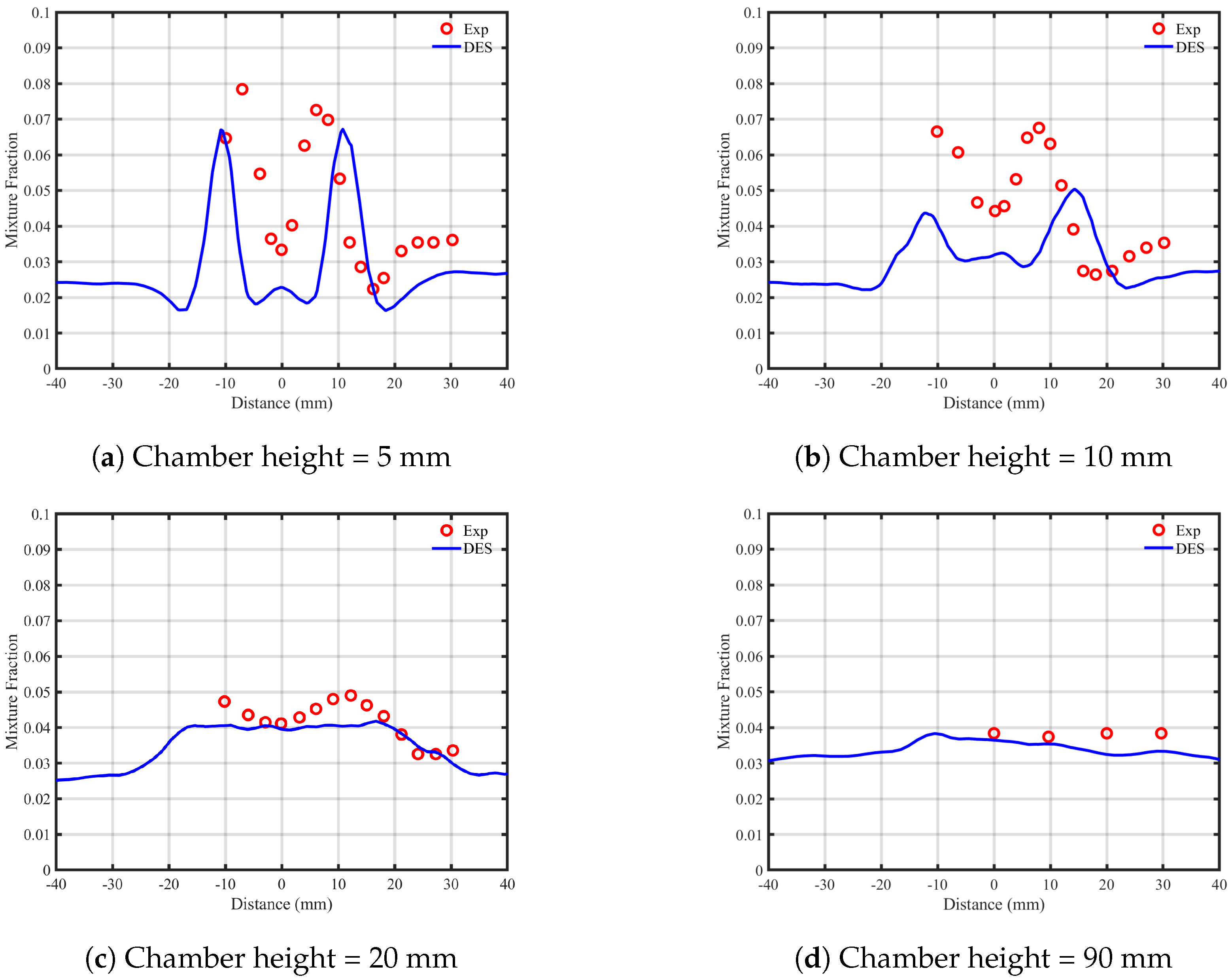
Figure 15 compares the numerical and experimental time-averaged mixture-fraction profiles. The mixture fraction reaches its maximum value above the fuel-nozzle exit, and the mean mixture fraction at the height of 5 mm is relatively low due to the nozzle configuration’s rapid mixing. The maximum simulated mixture fraction is
. The stoichiometric mixture fraction is reached at y = 5 mm and y = 10 mm, suggesting that the flame is not in equilibrium in these regions due to the low temperatures.
Interestingly, the mixture fraction in the IRZ is higher than the global value (), while the ORZ mixture fraction is equal to . This difference implies that the increase in mixture fraction in the IRZ benefits ignition and flame stabilization, allowing temperatures above the global adiabatic flame temperature.
The time-averaged plots at h = 20 mm show a reduction in variation along the y-axis of the mixture fraction, indicating rapid mixing of the fuel stream. The broadened maximum of the mixture fraction suggests that the mixing process is enhanced. Finally, at h = 90 mm, the mixing is complete in the time-averaged plots, and the mixture fraction profile becomes uniform. Overall, the simulation and experimental results are in good agreement, except for the mixture fraction at a height of 5 mm, where the simulation underestimates the experimental values.
The IRZ, the region of the flame where combustion is mainly completed, exhibits higher temperature levels and a mixture fraction that exceeds the global value of . This is due to the efficient mixing of the fuel and air in this region, which allows for complete combustion and elevated temperatures. This is important for efficient energy conversion and reduced emissions in combustion systems.
4.3.3. Methane Mass Fraction
Figure 13C shows the time-averaged distribution of the methane mass fraction. The numerical results presented in
Figure 16 are in good agreement with the experimental data. The plots reveal that the highest
mass-fraction values are found above the fuel-nozzle exit, indicating the presence of unburned fuel in this region. At y > 15 mm, the methane mass fraction drops to approximately 1% or less in all axial positions. This decrease is due to the rapid mixing of the fresh methane stream with the hot combustion products. Notably, no
was detected in the exhaust gas region, indicating that the combustion process is efficient. Close to the nozzle, the mass-fraction fluctuations reach
= 0.075, a relatively high value, but rapidly decreases to
= 0.0 at greater heights. This behavior is consistent with the rapid mixing and combustion of the fuel in the IRZ, which is characterized by high temperatures and a mixture fraction that exceeds the global value.
The simulated time-averaged mass fraction profiles agree with the experimental profiles at all positions. Similarly, the simulated turbulent mass-fraction fluctuation profiles generally match the experimental measurements, except for a slight overprediction at h = 20 mm. Notably, the distribution of other significant species, such as , , and , which are not represented here, also agrees well with the experimental results. Overall, these results demonstrate that the simulation accurately captures the behavior of the combustion process and provides valuable insights into the distributions and fluctuations of various chemical species.
4.3.4. Instantaneous Temperature
Figure 17A represent the instantaneous temperature distribution inside the combustion chamber. The contour plot clearly shows that the inner recirculation zone (IRZ) is unstable and exhibits temperature fluctuations. The higher-temperature gases in the IRZ are susceptible to transport toward the central nozzle, which can have a detrimental effect on the combustion process, as unburned gases may mix with the burned gases before re-entering the combustion chamber.
4.3.5. Instantaneous Methane Mass Fraction
The instantaneous mass fraction contour plot in
Figure 17 illustrates the flow dynamics of methane in the combustion chamber. The vortices in the shear layers play a crucial role in mixing the hot, burned gases from the outer recirculation zone (ORZ) and inner recirculation zone (IRZ) with the cold, unburned incoming gases. As the vortices break down, they generate smaller eddies, increasing the mixing rate and promoting flame stabilization.
Figure 17 also shows that the methane mass fraction is highest near the fuel nozzle and decreases rapidly with distance from it. The maximum methane mass fraction occurs at the interface between the ORZ and IRZ, where burned gases from the ORZ mix with unburned incoming gases from the IRZ. This suggests that the combustion process strongly depends on the reactants’ mixing rate and the transport of hot, burned gases into the incoming gas stream.
4.3.6. Instantaneous Heat Release
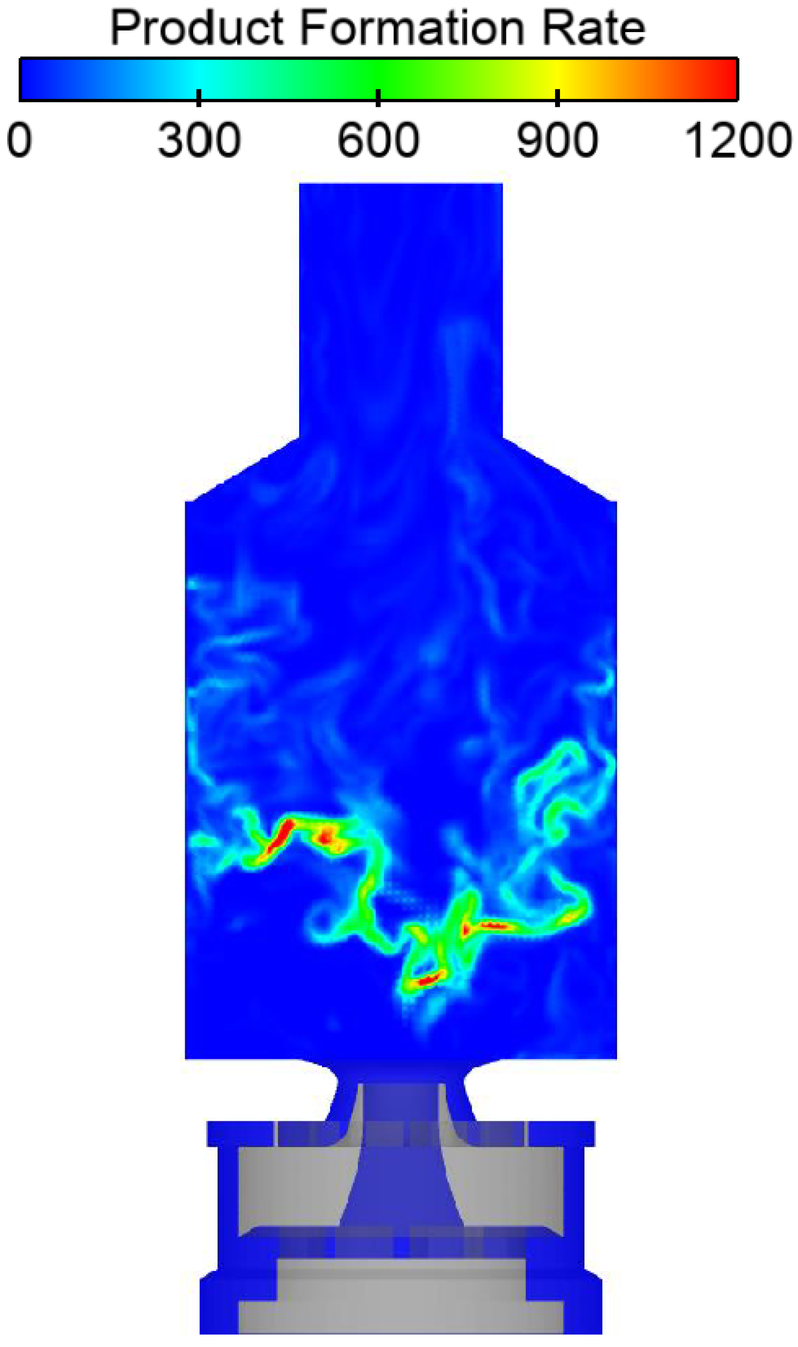
The combustion reaction primarily occurs in the inner and outer shear layers, where the burned gases from the outer recirculation zone (ORZ) and inner recirculation zone (IRZ) mix with the unburned incoming gas as represented in
Figure 18. The reaction zones are highly dynamic and vary in both space and time. In this case, the mixture fraction in the ORZ is below the global value, leading to generally low reaction rates in this region. However, due to mixing with the hot exhaust gases from the IRZ, the ORZ can contribute to the overall reaction.
The reaction zone in the IRZ is characterized by a mixture fraction exceeding the global value, which promotes higher temperatures and reaction rates, resulting in more complete combustion. Nonetheless, the reaction zones in both the ORZ and IRZ exhibit significant instability, with substantial variations in reaction rates and flame fronts.
4.4. Temperature–Mixture Fraction Correlation Analysis
The correlation between the temperature and mixture fraction of the flame at various heights (5 mm, 10 mm, and 15 mm) in the combustion chamber is represented in
Figure 19. The different radial zones are color-coded, spanning from 0 to 30 mm in radius. The solid lines indicate the strained laminar counterflow diffusion calculations (yellow) and adiabatic equilibrium (black) results. The numerical simulation utilizes a partially premixed module that consists of mixture fractions and a progress variable. The probability density function (PDF) table includes 20 species with a flammability limit of 0.1.
Although the investigation of partially premixed turbulent flames cannot be directly compared to counterflow diffusion flames, the calculated curves provide insight into the thermo-chemical state of the flames under examination. The mixture fraction disperses from to (equivalence ratio of ), with most samples between 0 and 0.1, indicating rapid mixing. At a height of 5 mm near the nozzle, the correlation between temperature and mixture fraction predominantly deviates from the equilibrium curve, indicating the absence of a well-defined mixture fraction in that region.
The maximum temperature in the outer recirculation zone (ORZ) reaches approximately 1400 K, while the peak value of the mixture fraction is around 0.03, which is well below the stoichiometric limit (). However, in the inner recirculation zone (IRZ), many samples are not yet ignited, with a significant number showing K, even around . This observation indicates that the flames are likely to be classified as partially premixed.
At heights of 15 mm and 30 mm, the highest temperature samples are primarily from the IRZ and are scattered between and K. These samples are located near the calculated curves, suggesting they are nearly completely burned. Furthermore, their mixture-fraction values exceed the global mixture fraction, indicating that fuel is more efficiently transported to the flame axes. This results in higher flame temperatures than the global adiabatic temperature for the global mixture fraction.
The IRZ plays a critical role in stabilizing swirl flames. Achieving a higher mixture fraction and temperature by adjusting the nozzle configuration can enhance the stabilization effect of the IRZ.
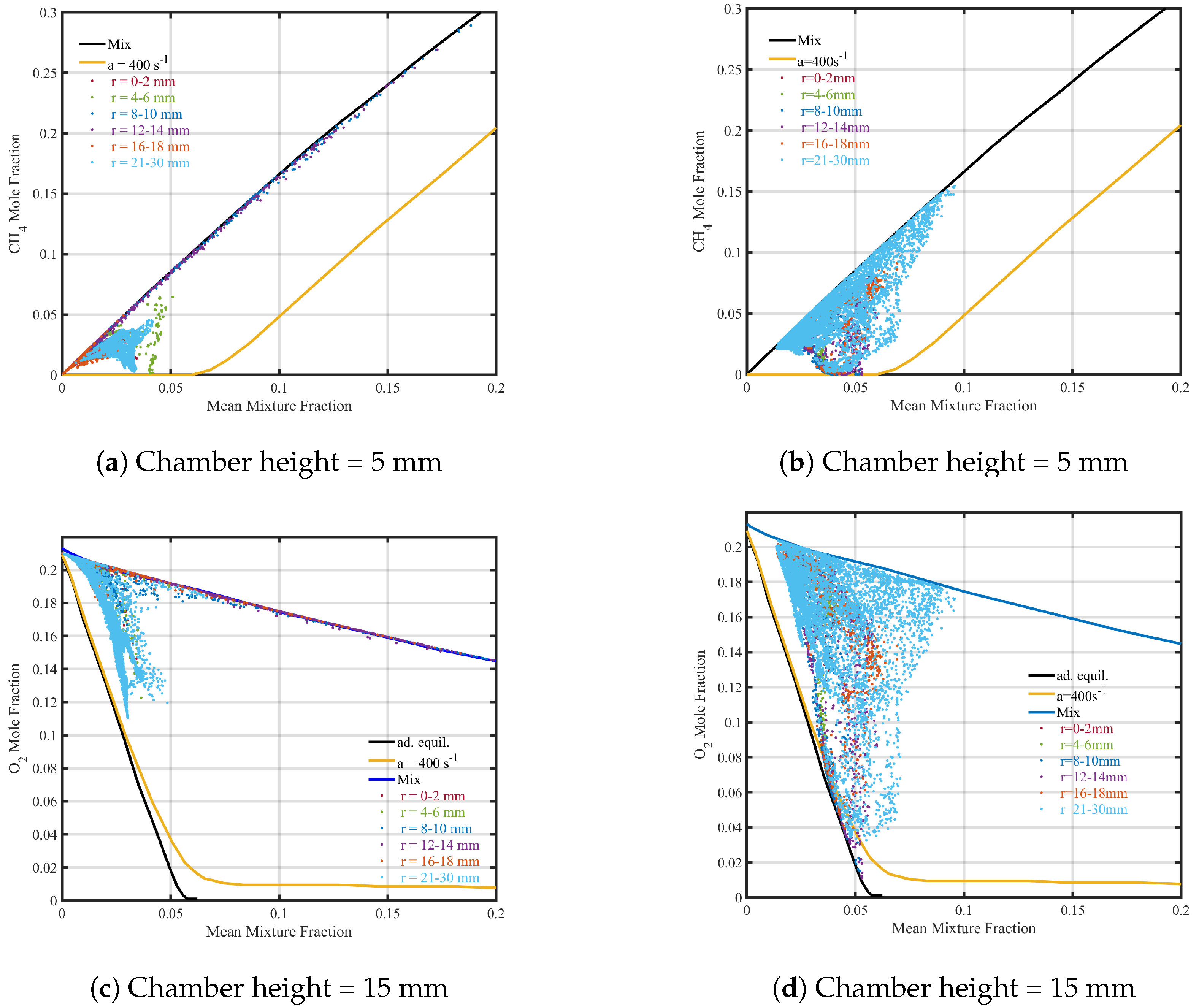
4.5. Species Mole Fraction
To a large extent, the species mole-fraction scatter plots agree with the scatter plots of temperature and the explanations provided above. The
and
results are shown in
Figure 20 as scatter plots at two different heights in the chamber (5 mm and 15 mm). A calculated curve representing the pure mixing of
and air is also included. Similar to the temperature scatter plots, the samples can be categorized into non-reacting, partially reacted, and fully reacted gas mixtures.
The fuel-rich samples deviate from the calculated curve of counterflow diffusion flames and align closely with the “Mix” curve. The mixture fraction of and further indicates that most samples from the radial region (–14 mm) follow the “Mix” curve, demonstrating a high degree of premixing.
The correlation between methane and oxygen is presented in
Figure 21, which directly illustrates the coexistence of fuel and air. Here, the samples with a methane mixture fraction of approximately zero are fully reacted, while all others follow the “Mix” curve, representing either pure mixing or partial reaction.
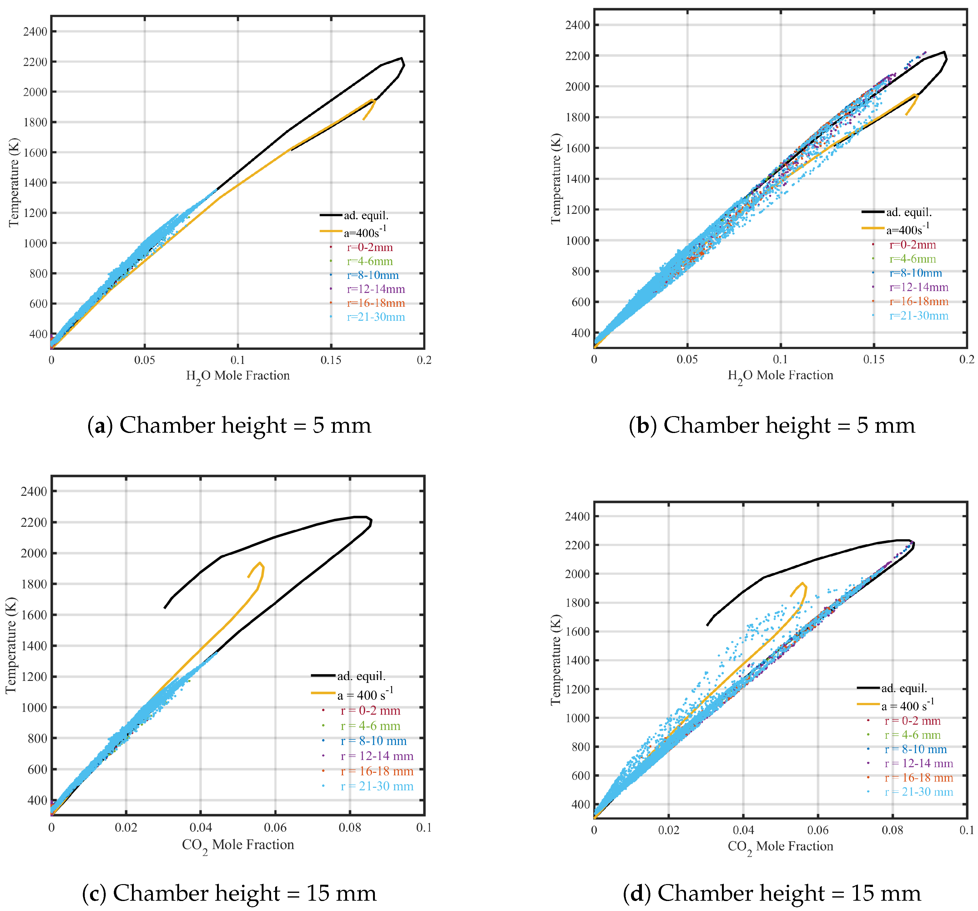
The correlation between temperature and carbon dioxide mole fraction at
mm and
mm is represented in
Figure 22. The results clearly show that the inner recirculation zone (IRZ) and the adjacent shear layer are in sensible agreement with adiabatic equilibrium. However, the calculation based on counterflow diffusion exhibits much poorer agreement, particularly for high CO
2 mole fractions.
5. Conclusions
This study investigated partially premixed flames using a partially premixed combustion model coupled with a detached-eddy simulation (DES) approach, focusing on methane and air combustion at an equivalence ratio of 0.65. The research aimed to validate the model’s ability to accurately simulate combustion dynamics in swirl-stabilized flames, a key feature of modern gas turbines. The numerical results were validated against experimental data, including time-averaged and root mean square velocity components, species profiles, mixture fractions, and temperature distributions. The comparison showed that the model captures the overall trends in the flow behavior, though minor discrepancies were observed, particularly in the adiabatic temperature region at lower mixture fractions. This indicates room for future improvements in the model, such as refinement of the PDF table values for more accurate predictions.
Additionally, the study provided insights into instantaneous flow structures and dynamic pressure changes, which deepen the understanding of the complexity and stability of the combustion process. The correlations between temperature, mixture fraction, and species concentrations were also explored, demonstrating the influence of these factors on combustion efficiency and stability.
One of the key contributions of this study is the significant reduction in computational cost. The proposed numerical setup is less computationally expensive than more detailed chemical mechanisms, offering a significant advantage in practical applications where rapid simulations are required. This reduction in computational cost represents a step towards sustainability, enabling faster design iterations and optimization without sacrificing essential accuracy. This is particularly relevant in the design and optimization of gas turbines, where computational efficiency is critical for real-time simulations and iterative design processes.
However, while the proposed model provides a good balance between accuracy and computational cost, there are limitations, particularly in the near-flame regions, where the model lacks the fine detail required for high-precision predictions. These discrepancies suggest that future studies should focus on improving the modeling of high-shear and near-flame regions, which could be addressed by refining the PDF values and exploring alternative turbulence–chemistry interaction models.
In short, this study presents a robust and computationally efficient methodology for simulating methane combustion in dual swirl combustors. While the model shows promise for gas turbine design and offers significant potential for sustainable engineering practices, further refinement is necessary for high-precision simulations in certain regions. Future work will aim to enhance model accuracy while maintaining computational efficiency, ultimately contributing to more sustainable and cost-effective design solutions in combustion engineering.
Author Contributions
Conceptualization, H.A.H.S., R.R. and A.M.; Methodology, G.M. and A.M.; Software, H.A.H.S.; Validation, H.A.H.S.; Formal analysis, H.A.H.S.; Resources, R.R.; Data curation, G.M.; Writing—original draft, H.A.H.S.; Writing—review and editing, G.M. and R.R.; Supervision, R.R.; Funding acquisition, G.M. All authors have read and agreed to the published version of the manuscript.
Funding
This research received no external funding.
Data Availability Statement
The original contributions presented in this study are included in the article. Further inquiries can be directed to the corresponding authors.
Acknowledgments
The author acknowledges the computational support provided by the Supercomputing Facility at SINES, NUST, Islamabad.
Conflicts of Interest
The authors declare no conflicts of interest.
References
- Mehdi, G.; Fontanarosa, D.; Bonuso, S.; De Giorgi, M.G. Ignition thresholds and flame propagation of methane-air mixture: Detailed kinetic study coupled with electrical measurements of the nanosecond repetitively pulsed plasma discharges. J. Phys. Appl. Phys. 2022, 55, 315202. [Google Scholar]
- Roux, S.; Lartigue, G.; Poinsot, T.; Meier, U.; Bérat, C. Studies of mean and unsteady flow in a swirled combustor using experiments, acoustic analysis, and large eddy simulations. Combust. Flame 2005, 141, 40–54. [Google Scholar]
- Galpin, J.; Naudin, A.; Vervisch, L.; Angelberger, C.; Colin, O.; Domingo, P. Large-eddy simulation of a fuel-lean premixed turbulent swirl-burner. Combust. Flame 2008, 155, 247–266. [Google Scholar] [CrossRef]
- Fiorina, B.; Vicquelin, R.; Auzillon, P.; Darabiha, N.; Gicquel, O.; Veynante, D. A filtered tabulated chemistry model for LES of premixed combustion. Combust. Flame 2010, 157, 465–475. [Google Scholar] [CrossRef]
- Moureau, V.; Domingo, P.; Vervisch, L. From large-eddy simulation to direct numerical simulation of a lean premixed swirl flame: Filtered laminar flame-pdf modeling. Combust. Flame 2011, 158, 1340–1357. [Google Scholar]
- Franzelli, B.; Riber, E.; Gicquel, L.Y.; Poinsot, T. Large eddy simulation of combustion instabilities in a lean partially premixed swirled flame. Combust. Flame 2012, 159, 621–637. [Google Scholar] [CrossRef]
- Chikishev, L.M.; Sharaborin, D.K.; Lobasov, A.S.; Dekterev, A.A.; Tolstoguzov, R.V.; Dulin, V.M.; Markovich, D.M. LES simulation of a model gas-turbine lean combustor: Impact of coherent flow structures on the temperature field and concentration of CO and NO. Energies 2022, 15, 4362. [Google Scholar] [CrossRef]
- Gregor, M.; Seffrin, F.; Fuest, F.; Geyer, D.; Dreizler, A. Multi-scalar measurements in a premixed swirl burner using 1D Raman/Rayleigh scattering. Proc. Combust. Inst. 2009, 32, 1739–1746. [Google Scholar]
- Janus, B.; Dreizler, A.; Janicka, J. Experiments on swirl stabilized non-premixed natural gas flames in a model gasturbine combustor. Proc. Combust. Inst. 2007, 31, 3091–3098. [Google Scholar]
- Fiorina, B.; Luu, T.P.; Dillon, S.; Mercier, R.; Wang, P.; Angelilli, L.; Ciottoli, P.P.; Hernández-Pérez, F.E.; Valorani, M.; Im, H.G.; et al. A joint numerical study of multi-regime turbulent combustion. Appl. Energy Combust. Sci. 2023, 16, 100221. [Google Scholar] [CrossRef]
- Popp, S.; Hartl, S.; Butz, D.; Geyer, D.; Dreizler, A.; Vervisch, L.; Hasse, C. Assessing multi-regime combustion in a novel burner configuration with large eddy simulations using tabulated chemistry. Proc. Combust. Inst. 2021, 38, 2551–2558. [Google Scholar] [CrossRef]
- Butz, D.; Hartl, S.; Popp, S.; Walther, S.; Barlow, R.S.; Hasse, C.; Dreizler, A.; Geyer, D. Local flame structure analysis in turbulent CH4/air flames with multi-regime characteristics. Combust. Flame 2019, 210, 426–438. [Google Scholar]
- Sloan, D.G.; Smith, P.J.; Smoot, L. Modeling of swirl in turbulent flow systems. Prog. Energy Combust. Sci. 1986, 12, 163–250. [Google Scholar] [CrossRef]
- Widenhorn, A.; Noll, B.; Aigner, M. Numerical study of a non-reacting turbulent flow in a gas-turbine model combustor. In Proceedings of the 47th AIAA Aerospace Sciences Meeting Including the New Horizons Forum and Aerospace Exposition, Orlando, FL, USA, 5–8 January 2009; p. 647. [Google Scholar]
- Benim, A.C.; Escudier, M.P.; Nahavandi, A.; Nickson, K.; Syed, K.J. DES Analysis of Confined Turbulent Swirling Flows in the Sub-critical Regime. In Proceedings of the Advances in Hybrid RANS-LES Modelling, Corfu, Greece, 17–18 June 2007; Peng, S.H., Haase, W., Eds.; Springer: Berlin/Heidelberg, Germany, 2008; pp. 172–181. [Google Scholar]
- Strelets, M. Detached eddy simulation of massively separated flows. In Proceedings of the 39th Aerospace Sciences Meeting and Exhibit, Reno, NV, USA, 8–11 January 2001; p. 879. [Google Scholar]
- Pope, S.B. Turbulent flows. Meas. Sci. Technol. 2001, 12, 2020–2021. [Google Scholar]
- Weigand, P.; Meier, W.; Duan, X.R.; Stricker, W.; Aigner, M. Investigations of swirl flames in a gas turbine model combustor: I. Flow field, structures, temperature, and species distributions. Combust. Flame 2006, 144, 205–224. [Google Scholar]
- Meier, W.; Duan, X.R.; Weigand, P. Investigations of swirl flames in a gas turbine model combustor: II. Turbulence–chemistry interactions. Combust. Flame 2006, 144, 225–236. [Google Scholar]
- Spalart, P.R. Strategies for turbulence modelling and simulations. Int. J. Heat Fluid Flow 2000, 21, 252–263. [Google Scholar]
- Noll, B.; Schütz, H.; Aigner, M. Numerical simulation of high-frequency flow instabilities near an airblast atomizer. In Proceedings of the Turbo Expo: Power for Land, Sea, and Air, New Orleans, LA, USA, 4–7 June 2001; American Society of Mechanical Engineers: New York, NY, USA; Volume 78514, p. V002T02A008. [Google Scholar]
- Ansys Fluent. Ansys Fluent Theory Guide; Ansys Inc.: Canonsburg, PA, USA, 2011; Volume 15317, pp. 724–746. [Google Scholar]
- Glassman, I.; Yetter, R.A.; Glumac, N.G. Combustion; Academic Press: Cambridge, MA, USA, 2014. [Google Scholar]
- Chen, Z.X.; Langella, I.; Swaminathan, N.; Stöhr, M.; Meier, W.; Kolla, H. Large Eddy Simulation of a dual swirl gas turbine combustor: Flame/flow structures and stabilisation under thermoacoustically stable and unstable conditions. Combust. Flame 2019, 203, 279–300. [Google Scholar] [CrossRef]
- Widenhorn, A.; Noll, B.; Stöhr, M.; Aigner, M. Numerical investigation of a laboratory combustor applying hybrid RANS-LES methods. In Advances in Hybrid RANS-LES Modelling; Springer: Berlin/Heidelberg, Germany, 2008; pp. 152–161. [Google Scholar]
- Syred, N. A review of oscillation mechanisms and the role of the precessing vortex core (PVC) in swirl combustion systems. Prog. Energy Combust. Sci. 2006, 32, 93–161. [Google Scholar]
- Widenhorn, A.; Noll, B.; Stöhr, M.; Aigner, M. Numerical characterization of the non-reacting flow in a swirled gasturbine model combustor. In High Performance Computing in Science and Engineering07; Springer: Berlin/Heidelberg, Germany, 2008; pp. 431–444. [Google Scholar]
- Stopper, U.; Aigner, M.; Meier, W.; Sadanandan, R.; Stöhr, M.; Kim, I.S. Flow field and combustion characterization of premixed gas turbine flames by planar laser techniques. J. Eng. Gas Turbines Power 2009, 131, 021504. [Google Scholar]
Figure 1.
The numerical domain of the gas turbine model combustor encompasses both the boundary conditions and measurement locations.
Figure 1.
The numerical domain of the gas turbine model combustor encompasses both the boundary conditions and measurement locations.
Figure 2.
(a) The top image depicts the grid, the middle image shows the ratio of the required length to the delta, and the bottom image displays the iso-surface of the integral length colored according to the velocity at a value of 5. (b) Wall y+ contour plot along the wall of the combustor.
Figure 2.
(a) The top image depicts the grid, the middle image shows the ratio of the required length to the delta, and the bottom image displays the iso-surface of the integral length colored according to the velocity at a value of 5. (b) Wall y+ contour plot along the wall of the combustor.
Figure 3.
The figure represents the contour plot and streamlines of the mean axial velocity.
Figure 3.
The figure represents the contour plot and streamlines of the mean axial velocity.
Figure 4.
Time-averaged axial velocity profiles (
left) and root mean square values (RMS) of radial velocity profiles (
right). The red dots represent the LDA measurements, and blue lines are numerical values (Widenhorn et al. [
14] and Chen et al. [
24]).
Figure 4.
Time-averaged axial velocity profiles (
left) and root mean square values (RMS) of radial velocity profiles (
right). The red dots represent the LDA measurements, and blue lines are numerical values (Widenhorn et al. [
14] and Chen et al. [
24]).
Figure 5.
Time-averaged radial velocity profiles (
left) and root mean square values (RMS) of radial velocity profiles (
right). The red dots represent the LDA measurements, and blue lines are numerical values (Widenhorn et al. [
14] and Chen et al. [
24]).
Figure 5.
Time-averaged radial velocity profiles (
left) and root mean square values (RMS) of radial velocity profiles (
right). The red dots represent the LDA measurements, and blue lines are numerical values (Widenhorn et al. [
14] and Chen et al. [
24]).
Figure 6.
The figure compares time-averaged tangential velocity profiles (
left) and root mean square (RMS) tangential velocity profiles (
right). Red dots denote experimental data from laser Doppler anemometry (LDA) measurements, while blue lines represent numerical simulation results (Widenhorn et al. [
14] and Chen et al. [
24]).
Figure 7.
Instantaneous axial-velocity contour plane at different time steps, visualized by streamlines and solid black lines indicating the zero-velocity location.
Figure 7.
Instantaneous axial-velocity contour plane at different time steps, visualized by streamlines and solid black lines indicating the zero-velocity location.
Figure 8.
Mean and instantaneous axial-velocity planes at x = 0, representing re-circulation zones with black solid lines and the point of separation.
Figure 8.
Mean and instantaneous axial-velocity planes at x = 0, representing re-circulation zones with black solid lines and the point of separation.
Figure 9.
Variable-pressure iso-surfaces colored according to the axial velocity at a constant time step.
Figure 9.
Variable-pressure iso-surfaces colored according to the axial velocity at a constant time step.
Figure 10.
Pressure iso-surfaces colored according to the axial velocity at different time steps.
Figure 10.
Pressure iso-surfaces colored according to the axial velocity at different time steps.
Figure 11.
Vortical structure colored according to the axial velocity, representing the pressure on the iso-surface.
Figure 11.
Vortical structure colored according to the axial velocity, representing the pressure on the iso-surface.
Figure 12.
Vorticity plane at x = 0.
Figure 12.
Vorticity plane at x = 0.
Figure 13.
Two-dimensional x–y mean contour plane of (A) temperature, (B) mixture fraction, and (C) CH4 fraction.
Figure 13.
Two-dimensional x–y mean contour plane of (A) temperature, (B) mixture fraction, and (C) CH4 fraction.
Figure 14.
Numerical profiles of time-averaged and RMS temperature along the center line compared with experimental results of time-averaged and RMS profiles.
Figure 14.
Numerical profiles of time-averaged and RMS temperature along the center line compared with experimental results of time-averaged and RMS profiles.
Figure 15.
Blue lines are numerical profiles of the time-averaged mixture fraction, and the red dots are LDA measurements at different heights of chamber.
Figure 15.
Blue lines are numerical profiles of the time-averaged mixture fraction, and the red dots are LDA measurements at different heights of chamber.
Figure 16.
Blue lines are numerical profiles of the time-averaged mass fraction of , and the red dots are LDA measurements at different heights of chamber.
Figure 16.
Blue lines are numerical profiles of the time-averaged mass fraction of , and the red dots are LDA measurements at different heights of chamber.
Figure 17.
Two-dimensional x–y instantaneous contour plane of (A) temperature, (B) mixture fraction, and (C) methane mass fraction.
Figure 17.
Two-dimensional x–y instantaneous contour plane of (A) temperature, (B) mixture fraction, and (C) methane mass fraction.
Figure 18.
Two-dimensional x-y contour plane of the product formation rate.
Figure 18.
Two-dimensional x-y contour plane of the product formation rate.
Figure 19.
Correlation between the temperature and mixture fraction of the flame at three different chamber heights. The colors represent different radial zones.
Figure 19.
Correlation between the temperature and mixture fraction of the flame at three different chamber heights. The colors represent different radial zones.
Figure 20.
Correlations between methane and mixture fraction and oxygen and mixture fraction at different heights.
Figure 20.
Correlations between methane and mixture fraction and oxygen and mixture fraction at different heights.
Figure 21.
Correlation between methane and oxygen at different heights.
Figure 21.
Correlation between methane and oxygen at different heights.
Figure 22.
Correlations between water mole faction and temperature and between carbon dioxide mole fraction and temperature at different heights.
Figure 22.
Correlations between water mole faction and temperature and between carbon dioxide mole fraction and temperature at different heights.
Table 1.
Comparison of peak time-averaged velocities and RMS values at different heights in the combustion chamber.
Table 1.
Comparison of peak time-averaged velocities and RMS values at different heights in the combustion chamber.
| Height (mm) | Axial Velocity (m/s) | Radial Velocity (m/s) | Tangential Velocity (m/s) | RMS—Axial (m/s) | RMS—Radial (m/s) | RMS—Tangential (m/s) |
|---|
| 5 | 30 (Simulated)
| 19 (Simulated) | 25 (Simulated) | 27 (Simulated) | 23 (Simulated) | 14 (Simulated) |
| 39 (Experimental) | 12 (Experimental) | 30 (Experimental) | 26 (Experimental) | 23 (Experimental) | 16 (Experimental) |
| 10 | 25 (Simulated) | 15 (Simulated) | 20 (Simulated) | 21 (Simulated) | 22 (Simulated) | 12 (Simulated) |
| 35 (Experimental) | 20 (Experimental) | 20 (Experimental) | 21 (Experimental) | 21 (Experimental) | 13 (Experimental) |
| 20 | 19 (Simulated) | 15 (Simulated) | 15 (Simulated) | 17 (Simulated) | 17 (Simulated) | 13 (Simulated) |
| 35 (Experimental) | 19 (Experimental) | 19 (Experimental) | 17 (Experimental) | 16 (Experimental) | 14 (Experimental) |
| 90 | 20 (Simulated) | 10 (Simulated) | 17 (Simulated) | 10 (Simulated) | 11 (Simulated) | 11 (Simulated) |
| 19 (Experimental) | 10 (Experimental) | 17 (Experimental) | 7 (Experimental) | 11 (Experimental) | 10 (Experimental) |
| Disclaimer/Publisher’s Note: The statements, opinions and data contained in all publications are solely those of the individual author(s) and contributor(s) and not of MDPI and/or the editor(s). MDPI and/or the editor(s) disclaim responsibility for any injury to people or property resulting from any ideas, methods, instructions or products referred to in the content. |
© 2025 by the authors. Licensee MDPI, Basel, Switzerland. This article is an open access article distributed under the terms and conditions of the Creative Commons Attribution (CC BY) license (https://creativecommons.org/licenses/by/4.0/).


