Abstract
In recent years, the semiconductor industry has embraced advanced artificial intelligence (AI) techniques to facilitate intelligent manufacturing throughout their organizations, with particular emphasis on virtual metrology (VM) systems. Nonetheless, the practical application of data-driven virtual metrology for product quality inspection encounters notable hurdles, such as annotating inspections in highly dynamic industrial environments. This leads to complexities and significant expenses in data acquisition and VM model training. To address the challenges, we delved into transfer learning (TL). TL offers a valuable avenue for knowledge sharing and scaling AI models across various processes and factories. At the same time, research on transfer learning in VM systems remains limited. We propose a novel parameter transfer learning (PTL) architecture for VM systems and examine its application in industrial process automation. We implemented cross-factory and cross-recipe transfer learning to enhance VM performance and offer practical advice on adapting TL to meet individual needs and use cases. By leveraging extensive data from Seagate wafer factories, known for their large-scale and high-dimensional nature, we achieved significant PTL performance improvements across multiple performance metrics, with the true positive rate (TPR) increasing by 29% and false positive rate (FPR) decreasing by 43% in the cross-factory study. In contrast, in the cross-recipe study, TPR increased by 27.3% and FPR decreased by 6.5%. With our proposed PTL architecture and its performance achievements, insufficient data from the new manufacturing sites, new production lines and new products are addressed with shorter VM model training time and smaller computational power with strong final quality prediction confidence.
1. Introduction
Machine learning (ML) has significantly enhanced the capabilities of intelligent manufacturing systems over the past few years. This improvement is particularly notable in industrial automation, where novel data-driven methodologies, such as predictive maintenance, computer vision, and anomaly detection, have played a pivotal role in advancing the development of systems that exhibit greater ease and robustness in automation than ever before. However, according to the recent survey of semiconductor device makers conducted by Mckinsey [1], only about 30% of respondents stated that they are already generating value through ML, while the other 70% are still in the pilot phase with ML and their progress has stalled. The production of semiconductors and microelectronics entails the use of highly complex and expensive equipment, and intricate fabrication processes that require a high degree of precision. To reduce costs, improve yields, and increase the overall fab throughput, these device makers actively leverage advanced machine learning techniques in multiple specific use cases, such as visual inspection, defect identification, root cause analysis, virtual metrology (VM), etc. This paper focuses on the scalability of ML-based virtual metrology models for semiconductor and microelectronics manufacturing.
The semiconductor manufacturing process is characterized by high fragmentation, with a diverse range of products flowing through production lines. This requires using complex machines and multiple process recipes and steps. In a certain process recipe, engineers typically specify one constant time frame for each step. However, the variability in individual wafers may introduce statistical or systematic fluctuations in the time frame required for a given step. A process could keep running until it has achieved the desired outcome, leading to an increase in both timelines and resource waste and potentially even chip damage. To improve processing accuracy, semiconductor companies leverage live tool-sensor data and tool-sensor readings from previous process steps, allowing machine learning models to capture nonlinear relationships between processes and wafer-inspection outcomes (measured by a metrology system).
Metrology is the science of measuring and characterizing tiny structures and materials. Metrology systems are responsible for ensuring production quality in the semiconductor manufacturing industry. Offline sampling inspection is a widely used method to achieve quality control goals. However, this approach can only evaluate the quality of a limited number of sampled wafers, resulting in a waiting period to obtain metrology values after the completion of the manufacturing process. The delay associated with metrology acquisition in offline sampling inspection precludes real-time monitoring of product quality, thus reducing the effectiveness. To overcome time and cost limitations involved by offline sampling, VM systems have been developed to predict metrology variables based on process and wafer state information [2]. A machine learning-based virtual metrology system, made possible by advancements in machine learning techniques, can be trained to automatically detect and classify defects on wafers with comparable or superior accuracy to human inspectors. Additionally, specialized hardware, such as tensor-processing units, and cloud [3] offerings enable the automated training of machine learning algorithms at scale. This, in turn, allows quicker piloting, real-time inference, and scalable deployment of VM systems.
In recent times, VM has garnered substantial attention from researchers, and its effectiveness in wafer inspection has been demonstrated through several studies, including a locally weighted partial least squares approach for the dry etching process [4], Gaussian process regression models for the chemical mechanical polishing process [5], etc. Recently, soft-sensing ConFormer [6] was developed in the first empirical study of wafer inspection, based on semiconductor manufacturing data provided by the IEEE BigData 2021 Cup in Soft Sensing at Scale-Seagate [2].
However, the practical implementation of VM models in deep learning is impeded by two distinct characteristics: First, ML algorithms assume that training and testing data originate from the same probability distribution. It is imperative that the training dataset and the actual problem are similar in terms of their feature space and the distribution of data therein. However, this assumption may not hold in reality as data collected from different production contexts is likely to arise from different probability distributions. Moreover, it is noteworthy that machine learning algorithms are limited to learning only the effects that are present in the training data. Consequently, the efficacy of these algorithms is reliant on the quality and quantity of the data, which must be large and diverse in order to include rare events as well. In practice, acquiring such comprehensive datasets is increasingly arduous and complex as problems become more intricate. Second, retraining an ML-based VM model once trained is similar to training a completely untrained one. It necessitates a substantial amount of computational power and access to all of the training data. In the context of a highly dynamic industrial automation environment such as an semiconductor manufacturer where production lines regularly switch between products, tools, or processes, this approach is impractical.
Transfer learning (TL) offers a potential solution to mitigate both issues at hand. TL refers to a collection of techniques that aim to reduce the volume and caliber of necessary data while simultaneously enabling the utilization of prior knowledge instead of commencing each learning task from scratch. This is accomplished by transferring knowledge between tasks, thus producing distributed cooperative learning systems. Although transfer learning has been extensively studied in areas such as medical imaging, spam detection, and speech recognition, there appears to be a lack of similar research in the semiconductor and microelectronics industrial automation sector.
We investigate the value of the transfer learning approach within the context of semiconductor manufacturing. The objective was to achieve a more precise virtual metrology model that could effectively manage data scarcity across a variety of processing scenarios. Specifically, this study introduces a TL method that utilizes parameter transfer. Parameter transfer enables the adaptation of a machine learning model to variations in the feature space arising from differences in the types and number of sensors used in the process monitoring system, without requiring complete retraining of the algorithm [7]. It has been adopted in quality management [8], anomaly detection [9,10], etc. The proposed approach involves reusing a pre-trained deep neural network from the source domains to enhance the predictive capability in the target domains, thereby reducing the requirement for extensive training data in the target domains. The TL used in the study is based on soft-sensing ConFormer (CONvolutional transFORMER) [6], which is a VM model that underpins transfer learning for wafer fault diagnostic. This model comprises multi-head convolution modules that leverage the benefits of fast and lightweight convolution operations while also being capable of learning robust representations through multi-head design akin to transformers.
In this paper, performances of different TL tasks—cross-factory and cross-recipe—are evaluated with a focus on the key parameters of the successful strategies. Numerical experiments are conducted on real-world industrial semiconductor manufacturing data provided by Seagate wafer factories.
2. Preliminaries
Aligned with the objective of the current study, this section presents a review of the limited existing literature pertaining to transfer learning within the context of virtual metrology. In [11], the authors propose a unified VM model for two identically designed chambers utilizing a deep learning architecture, specifically a domain adversarial neural network. This model incorporates a discriminator that distinguishes between the two chambers during the examination process. In [12], the use of TL techniques was explored for equipment with identical design in scenarios where the number of wafer records for the target equipment is inadequate. A VM modeling approach based on the paradigm of transfer learning in a fragmented production context was presented in [13], which exploits a convolutional neural network (CNN)-based spatial pyramid pooling model to perform the TL with inputs of different sizes. Hsieh et al. [14] proposed an automated VM (AVM) server that also employs CNNs for efficient VM processing, which was achieved by optimizing the CNN architecture and developing an automated data alignment scheme to align the inputs, enhancing the feasibility of deployment. Based on that, an advanced AVM system [15] based on a convolutional autoencoder and TL was proposed to address the practical application challenge, i.e., insufficient metrology data and online model refreshing. Experimental results confirmed the feasibility of employing the advanced AVM system for onsite applications in actual production lines.
However, given the limited literature related to TL in VM, there are insufficient guidelines to find a good exemplary TL application to achieve scalable VM in semiconductor manufacturing. This paper aims to offer insights into the adaptability of scalable deep learning-based VM with a pragmatic transfer learning approach to the specific requirements of diverse industrial processes.
2.1. Transfer Learning
Transfer learning is a field that explores and develops machine learning methods by leveraging knowledge gained from previously solved source tasks to more efficiently solve new target tasks. In the published literature, inconsistencies remain in transfer learning terminology. Regarding labeled data availability, three common problem categories are distinguished:
- Inductive transfer learning target is where domain labels are provided.
- Transductive transfer learning is where only the source domain labels are available.
- Unsupervised transfer learning is where neither source nor target domain labels are available.
Accordingly, four main approach categories are defined among statistical transfer learning and deep transfer learning approaches:
- Instance transfer learning describes approaches that add (weighted) instances from the source domain(s) to the target domain to improve training on the target task.
- Feature representation transfer learning involves mapping instances from both the source and target domains into a shared feature space. This approach can enhance training for the target task.
- Parameter transfer learning involves sharing parameters or priors between source and target domain models to enhance the initial model before training on the target task. In deep transfer learning, this is achieved through the partial reuse of deep neural networks pre-trained on the source domain(s).
- Relational knowledge transfer learning maps relational knowledge from the source to the target domains, which usually requires domain expertise. However, deep transfer learning using generative adversarial networks or end-to-end approaches can alleviate this issue by integrating domain adaptation into the decision-making function.
The applicability of different approach categories in a real-world setting depends on specific factors such as dataset and storage sizes, communication bandwidth, and the availability of expert knowledge. It is important to note that this applicability is not solely determined by the advantages or disadvantages of the approaches in general or the categorization of the problem, as described above.
Parameter transfer learning (PTL) fundamentally involves the transfer of model parameters, specifically weights and biases, from a pre-trained model within a source domain to a new model in a target domain. In contrast, traditional transfer learning predominantly emphasizes the transfer of data instances from the source domain to the target domain, adjusting the model’s weights during the target domain’s training process. The principal advantage of PTL over traditional transfer learning lies in its ability to significantly reduce both the training time and the computational resources required to retrain the target model, thereby enhancing efficiency and scalability in model deployment.
The application of parameter transfer learning (PTL) in industrial process automation is constrained by the necessity for congruence between the source and target domains. Specifically, the industrial processes in both domains must exhibit similar features or tasks to ensure effective knowledge transfer. For instance, implementing PTL in a new factory’s process automation (target domain) necessitates that the setup processes closely resemble those of an existing factory (source domain). This requirement for similarity poses a significant limitation, as it restricts the versatility and broader applicability of PTL in diverse industrial settings where process characteristics may differ substantially.
2.2. Virtual Metrology
In a bid to explore the practicality of implementing virtual metrology in its manufacturing operations, Seagate Technology conducted a comprehensive study utilizing a large volume of tool-sensor data from multiple manufacturing sites worldwide. As part of this study, the Seagate researchers proposed an autoencoder-based model that achieved dimension reduction and virtual metrology prediction simultaneously. The virtual metrology problem is complex and requires the utilization of large-scale deep learning models, particularly in scenarios involving time-series data. Incorporating sensor data sequences into the model enhances its predictive capabilities, but it simultaneously necessitates a more intricate design for models. To this end, the researchers developed the soft-sensing transformer model, which leverages self-attention mechanisms that have been proven to be effective for sequential data and efficient for high-dimensional inputs. However, while the soft-sensing transformer model demonstrated exceptional performance on some virtual metrology tasks in Seagate’s sensor data, it was unable to uncover correlations between sensors. The gaps in correlation and interpretability were filled by the ConFormer [6] model. ConFormer combines convolutional networks and transformers to extract the local correlation between neighbor features (sensors) and enhance accuracy while building upon this idea and incorporates correlations between all sensors through a graph neural network. The ConFormer model exhibits impressive capabilities in prediction performance and feature correlation extraction. DeepViz is a technique that visualizes features importance and can be applied to all the aforementioned models. By visualizing importance, DeepViz not only facilitates the interpretation of how the models make predictions but also provides a means of improving model performance by assigning higher weights to more important features. In addition, the researchers at Seagate conducted a thorough investigation of model training and data processing techniques, yielding valuable insights in this regard.
2.3. Problem Formulation: Transfer Learning in Seagate Factories
Given a source domain and source learning task , a target domain and a target learning task , transfer learning aims to help improve the learning of the target predictive function (VM model) in by using the knowledge in and , where .
In the given definition, a domain is a pair , where is the feature or sensor space and is marginal probability distribution. Thus, the condition indicates that either or .
Motivated by the diversity of wafer manufacturing lines, we, therefore, propose the following two base use cases to examine best practice examples of TL and facilitate their adaption to other scenarios.
- Cross-factory refers to the transfer of knowledge and expertise from one location to another, as illustrated in Figure 1a. This practice involves leveraging the knowledge gained from one factory or site and applying it to other similar entities located elsewhere. This allows the dissemination of valuable knowledge and the sharing of best practices across different sites, ultimately improving overall performance and efficiency. In the realm of semiconductor manufacturing, a diverse range of deposition tools are utilized to create electronic components via the deposition of a thin film of material onto a substrate. They have the same process parameters, i.e., , while tools vary from each other and are located in different sites, resulting in different performance, i.e., ;
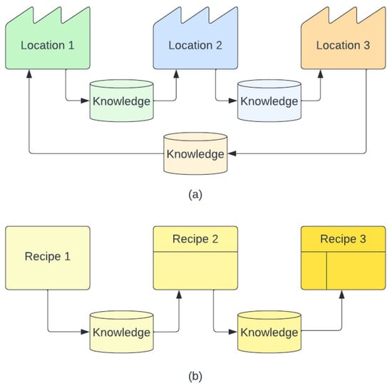 Figure 1. (a) Cross Factory Transfer Learning (b) Cross Recipe Transfer Learning.
 - Cross-recipe refers to the transfer of knowledge from one distinct manufacturing process recipe to another, for instance, from the processing of one product to a different one, , as illustrated in Figure 1b. A recipe in wafer manufacturing typically refers to a set of instructions detailing the specific steps and parameters required to fabricate a component at a given operation in the process flow. In this case, and .
It is noteworthy that, in the VM task perspective, the task can be defined as , where is the label space and is the predictive VM model that can be defined as . Taking deposition machining as an example, the film thickness on all the wafers are examined after the process finishes, i.e., . The different performances of different tools will result in variations in the thickness measurements; that is .
2.4. Manufacturing Data Acquisition
The wafer manufacturing process is a complex and time-consuming operation, involving numerous stages such as metal deposition, dielectric deposition, etching, electroplating, planarization, and lithography. The intricacy of the process makes it challenging to maintain manufacturing stability, hindering quality control in industrial production. In order to enhance the predictability of qualified product yield, a large sensor network is installed in the manufacturing line to monitor wafer quality. At each stage of processing, engineers collect and analyze multiple critical sensor records. These records provide data on key quality indicators that allow the engineers to assess the quality of the wafer. To do this, they use internal heuristic threshold values for each indicator. However, the sensor data collected are often highly nonlinear, dynamic, and noisy, making them difficult to handle. To overcome this challenge, Seagate wafer factories have adopted data-driven VM models [6,16]. These models use multivariate time-series sensor data to predict inspection results, specifically the pass or fail of binary indicators.
Specifically, the data are obtained from two manufacturing sites with similar processes. However, while the dataset from Factory 1 exhibits greater volume and diversity, the dataset from Factory 2 is relatively smaller in scale. The objective of this study is to facilitate the transfer of knowledge acquired from the larger and more diverse dataset at Factory 1 to the smaller dataset at Factory 2. We utilize datasets obtained from five distinct manufacturing process recipes spanning a duration of 2 years to train and validate the models. The test set, conversely, comprises data from a more recent time period and is divided into four periods of equal duration.
The sample size of the training and validation sets from Factory 1 and Factory 2, grouped according to five different process recipes, are presented in Figure 2. The ratio between the training set and validation set between Factory 1 and Factory 2 are less than 60% and 67%, respectively. Meanwhile, Figure 3 displays the sample size of the test sets across four distinct testing periods for both factories. The ratios between the test set between Factory 1 and Factory 2 are less than 72%.
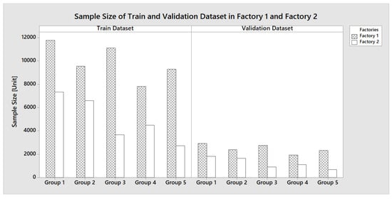
Figure 2.
Training and Validation Sample Sizes from Factory 1 and Factory 2.
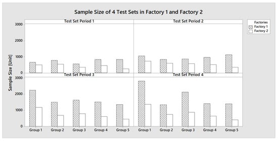
Figure 3.
Test Dataset Sample Sizes from 4 Test Periods from Factory 1 and Factory 2.
3. Materials and Methods
3.1. Virtual Metrology Base Model Architecture
The ConFormer (CONvolutional transFORMER) Model [6] is used as the baseline for the virtual metrology transfer learning model. The ConFormer architecture consists of 2 main components, a convolutional neural network (CNN) and multi-head self-attention layers [17]. The CNNs and multi-head self-attention mechanism are described in detail in Section 3.1.1 and Section 3.1.2, respectively.
The ConFormer Model is illustrated in Figure 4. The sensor data, as described in Section 2.4, are fed into a dense layer as an embedding layer to reduce the high-dimensional input data, which is expressed in Equation (1)
where is a sigmoid activation function, and FC(·) is a fully connected (FC) layer, i.e., dense layer.
The dense layer data output is fed to the multi-head self-attention layer, which is described in Section 3.1.2. In this ConFormer Model, there are three convolutional blocks, each of which consists of following layers:
- Gated linear unit (GLU) [18], which is expressed in Equation (2).where is a sigmoid activation function, and are weight parameters which are associated with previous input .
- Convolutional neural network (CNN), which is described in Section 3.1.1
- Batch Normalization [19], which is a layer to normalize activations in-between deep neural network layers. It also aims to improve deep learning model performance and speed up model training convergence.
- Swish activation layer [20], which can be calculated from Equation (3).where is a sigmoid activation function.
- Fully connected layer (also known as a dense layer), which is expressed in Equation (4)where W denotes weight parameters associated with input i, and denotes a bias parameter.
3.1.1. Convolutional Neural Network (CNN)
In the convolutional neural network (CNN), the convolution is performed by multiplying a filter or kernel with a data fragment at each point and moving the filter by n-strides along the X and Y directions of the data to complete the whole image. Feature maps are generated as a result. The stride is the number of hops by which the filter moves along the network [21].
Figure 5 shows a graphical explanation of the convolution process, where the input data have a shape of (7 × 7 × 1) and there are 3 kernels, , , and with a shape of 3 × 3 in the first convolutional layer. As the result, 3 feature maps , and are generated. In the second convolution layer, there are 3 kernels, namely, and for each channel with a kernel shape of 2 × 2 that are convoluted with the previous feature maps to obtain the next feature maps , and .
The convolution result can be expressed as in Equation (5)
where M is the number of feature maps, are the feature maps from the previous layer t, is kernel in the current layer, and denotes the bias in the current layer.
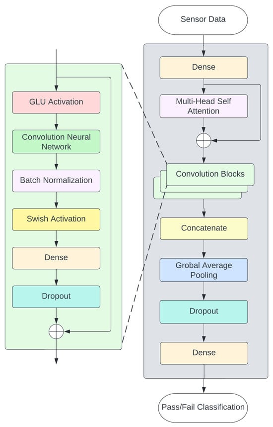
Figure 4.
ConFormer (CONvolutional transFORMER) Architecture.
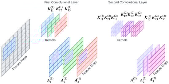
Figure 5.
Two-Layer Convolutional Neural Network with 3 Filters in Each Layer.
3.1.2. Multi-Head Self-Attention
Multi-head self-attention ws introduced by [17], and was first used in transformer models for natural language processing applications. Self-attention captures the dependency among input tokens, which is calculated by the scaled dot product between the Q and K input tokens, and the result is normalized by a softmax function with the response of the token V as expressed in Equation (6). The multi-head self-attention is a concatenation of each self-attention of the head, as described in Equation (6).
An alternative concise expression of the scaled dot product operation is also represented in Equation (7).
As shown in Figure 6a, an initial input of the scaled dot product attention is the input embedding with a size of matrix. Then, three matrices are generated from the input X:
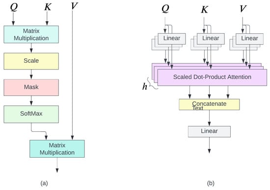
Figure 6.
(a) Scaled Dot Product Attention (b) Multi-Head Attention.
- The query (Q), matrix, where is a matrix, as a result, Q is a matrix.
- The key (K), matrix, where is a matrix, and K is a matrix. The scaled dot product between Q and K requires .
- The value (V), matrix where is a matrix, with a size of V.
The normalization by of the dot product between query (Q) vectors and key (K) vectors is required to control the dot product result magnitude. The large magnitude results in a softmax function in a region with a small gradient [22].
The benefit of the attention mechanism is that it does not have any recurrent connections and it can compute the input token in parallel in the same layer. As a result, it gains better effectiveness, efficiency, and scalability [23]. This parallel computation is also called multi-head attention, which is shown in Figure 6b and expressed in Equation (8)
where
3.2. Parameter Transfer Learning Architecture
This study aims to investigate the parameter transfer approach, a technique that employs a parametric model to encode and transfer knowledge. The central objective of this approach is to minimize the expected risk associated with the target task by leveraging relevant knowledge from an effective parameter in the source region and applying it to the target region. To accomplish this, we propose a strategy that entails learning an optimal parameter in the source region and transferring a subset of this parameter to the target region. One way to control the parameters involves directly constraining the parameters of the source model to the target model.
In this paper, as shown in Figure 7, the parameter transfer learning design is executed in two steps, pre-training followed by fine-tuning. In the first step, sufficient historical data collected from a variety of tools in the source domain are collected to build the initial model. After pre-training the VM model with sufficient qualified data, the ConFormer blocks within the VM model contain deep, discriminative convolutional filters that are learned from source domain data. However, due to different characteristics that exist among tools from different domains, the prediction accuracy may be poor when leveraging this initial model to other tools, even of the same type. Therefore, to further enhance the accuracy of pre-trained VM models on the target domain, the pre-trained model needs to be fine-tuned. However, during the fine-tuning process, the gradient is allowed to propagate back through the whole network, which may compromise the discriminative filters in the ConFormer blocks. To avoid this problem, it is recommended to freeze all convolutional layers within the VM model, while the final layers (the last FC layer and the softmax function) of the VM model are fine-tuned. In the context of convolutional neural networks, freezing layers refer to a technique used to control the weight update process. Specifically, by selectively freezing different numbers of convolutional layers, the weight behavior of the convolutional layers can be derived for the target model, holding all other factors constant. Finally, by fine-tuning the modifiable parameters until reaching the desired objective function, the re-trained VM model should be able to recognize different object types or classes in the target domain.
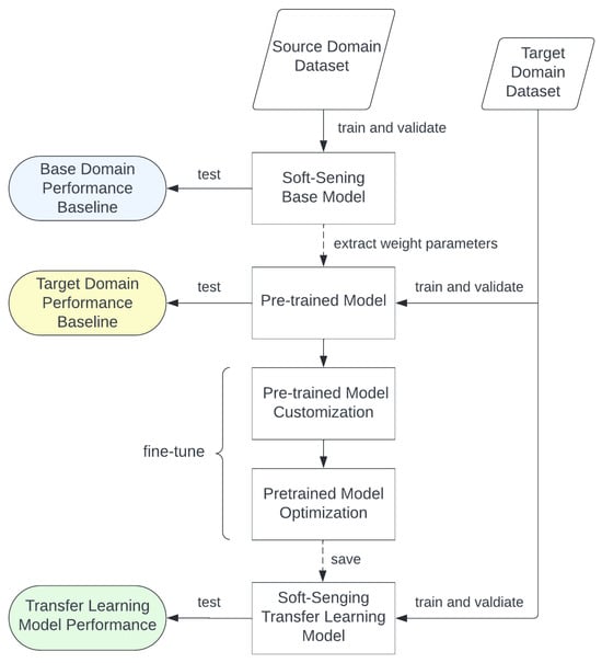
Figure 7.
Parameter Transfer Learning Architecture.
Key challenges associated with applying PTL in VM lie in the necessity for extensive pre-training of the source model on large-scale datasets. This pre-training is crucial, as it lays the groundwork for subsequent model optimization and fine-tuning processes. Such rigorous preparation is essential, as it directly influences the VM’s performance metrics, specifically the true positive rate (TPR), false positive rate (FPR), and area under the curve (AUC). Thus, the performance and efficacy of the VM are contingent upon these comprehensive and meticulous preparatory stages.
3.3. Experiment Setting
3.3.1. Design of Experiments
First, we aimed to investigate the effectiveness of transfer learning in the context of virtual metrology modeling with a cross-factory adaptation. Specifically, we employed datasets from two distinct factories, with those from factory 1 and factory 2 serving as the source domains and target domain, respectively. The utilization of Factory 2’s dataset as the target domain is of particular interest given its relatively small size. Such a scenario highlights the potential benefits of TL in addressing the issue of data scarcity. Second, a cross-recipe transfer learning experiment was conducted utilizing a dataset derived from two separate manufacturing process recipe groups. The source recipe group exhibited a greater degree of diversity than recipe groups 1 to 5. As such, the source recipe group was designated as the source domain, while recipe groups 1 to 5 were selected as the target domain for this particular experiment.
3.3.2. Evaluation Metrics
The evaluation of virtual metrology models’ performance involves assessing the true positive rate (TPR), false positive rate (FPR), and area under a receiver operating characteristics curve (AUC-ROC). This is carried out for models trained on the base domain, target domain, and with transfer learning [24]. According to Figure 8, the true positive rate (TPR), false positive rate (FPR), and AUC score can be expressed as in Equation (9), (10) and (11), respectively. Higher TPR and AUC are indicators of superior model performance, while a lower FPR suggests better model performance.
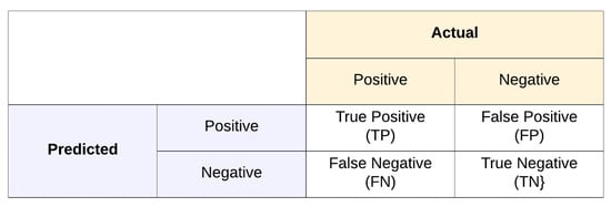
Figure 8.
Confusion Matrix.
A higher TPR indicates that PTL is effectively leveraging the knowledge gained from the pre-trained model to accurately identify true positive in the VM task. Conversely, a lower FPR shows that PTL directly increases precision in VM performance, meaning that the VM model’s positive predictions are more likely to be correct.
3.3.3. Implementation Details
The ConFormer model and its training methodology are utilized across all domains. The model was implemented in the Keras 2.3 framework. The optimal values were determined after comparing the results of various parameter choices. The embedding size was selected as 64, as it outperformed the other sizes in the pool of size parameters [32, 64, 128, 256]. To address overfitting, different dropout values ranging from no dropout to 0.8 dropout were tested, and a dropout value of 0.5 was found to be optimal. To further regularize the model, different values in the set [1e-3, 1e-4, 1e-5, 1e-6] were tested, and a regularization value of 1e-4 was chosen. The batch size was set as 1024. The optimization was performed using the Adam optimizer, with the scheduled learning rate set as in [6]. The early stopping mechanism was executed if the performance of the model on the validation dataset started to degrade (with patience being set at 50 epochs).
The transfer learning procedure realizing the idea of parameter transfer of deep VM models comprises the following steps:
- Source domain training and evaluation: The base model was trained on data from the source domain, from which the weight parameters of the model were preserved. In this step, the maximum epoch number is set as 2000. The increase in the number of epochs determines the model performance improvement [25]. The initial learning rate is set as 0.001. This pre-trained model serves as a pre-trained baseline.
- Target domain training and evaluation: the base model was trained separately on the target domain dataset using hyperparameter settings identical to those of the source domain.
- Parameter transfer and evaluation: The base model was initialized using the weights from the pre-trained baseline. The weight parameters of the three CNN layers discussed in Section 3.1 are frozen, which restricts learning and prevents weight parameter updates. Conversely, the input layer of a pre-trained model is unfrozen and it may be necessary to modify the input dimensions in cases where the data shapes of the source and target domains differ. A dense layer is appended to the final layer, creating a transfer learning model through fine-tuning. The partially frozen model is re-trained on the target domain, where the epoch is limited to 200, while the initial learning rate is reduced to . Thus, reducing the number of epochs not only decreases training time but also minimizes computational power consumption.
4. Results
In this section, the cross-factory transfer learning results are shown in Section 4.1 and cross-recipe transfer learning results are described in Section 4.2.
4.1. Cross-Factory Transfer Learning Results
The cross-factory VM transfer learning performance result is shown in Table 1. Due to the significantly larger and more diverse source domain dataset (factory 1), the model encounters difficulty in learning all the patterns. Therefore, the model’s performance on the source domain may not surpass that of the target domain, as evidenced in the first two columns of Table 1. The utilization of the parameter transfer learning approach aids in enhancing the performance of the VM model on the target domain (factory 2). For five different recipe groups of transfer learning from factory 1 to factory 2, the overall TPRs in the four test periods increased while FPRs decreased. Especially for Group 1, the average test TPR increased by while the average FPR decreased by 43%. The cross-factory performance improvement is shown in Figure 9.

Table 1.
Cross-Factory Transfer Learning Performance and Result.
However, it should be noted that cross-factory transfer learning may not consistently improve the performance of VM models. For instance, we observed a reduction in TPRs after transfer learning for Group 3 and Group 5, which can be attributed to the poor performance of the model in the source domain. Nevertheless, given the significant improvement in FPRs, such a reduction in TPRs is considered acceptable.
4.2. Cross-Recipe Transfer Learning Results
The VM performance on the source recipe domain is shown in Table 2. The cross-recipe transfer learning experiment result is shown in Table 3. By utilizing the knowledge in the source recipe group, we can significantly improve the performance of target recipe Groups 1 to 4. However, in target recipe Group 5, the average FPR on the test dataset significantly increased from 3.37% to 9.87%, while the average TPR improved from 55% to 82.3%. The cross-recipe performance improvement is shown in Figure 10.
Table 2.
Source Recipe Group Baseline Performance.
Table 3.
Cross-Recipe Transfer Learning Performance and Result.
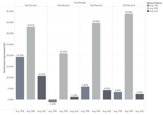
Figure 9.
Cross-Factory Performance Improvement.
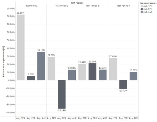
Figure 10.
Cross-Recipe Performance Improvement.
5. Conclusions
This study presents a parameter transfer learning approach for virtual metrology using extensive manufacturing data from Seagate Technology. The performance of our parameter transfer learning approach was evaluated on various datasets sourced from different factories, time periods, and processing recipes. With our PTL architecture, performance improved, with the true positive rate (TPR) increasing by 29% and the false positive rate (FPR) decreasing by 43% in a cross-factory study. In contrast, in a cross-recipe study, TPR increased by 27.3% but FPR decreased by only 6.5%. These results demonstrate that our parameter transfer learning approach can significantly enhance the manufacturing model’s quality prediction capability, particularly on insufficient datasets or datasets with limited diversity. Therefore, our approach not only enhances manufacturing processes where new manufacturing sites, new production lines, or new products have insufficient data for VM model training but also requires shorter model training time and smaller computational power to acquire a high true prediction rate.
6. Discussion
Although extensive datasets have been investigated, they constitute only a limited fraction of the complete Seagate manufacturing lines. Our future investigations will entail more in-depth modeling and the utilization of transfer learning across data from various product lines within Seagate. Therefore, manufacturing sites can apply our PTL approach to other manufacturing processes, e.g., wafer inspection.
Model parameters are meticulously optimized for each virtual metrology (VM) scenario. This optimization process necessitates a high degree of similarity in features, tasks, and operational conditions between the source domain and the target domain. Such congruence is essential to ensure that the knowledge transferred from the pre-trained model is effectively leveraged, thereby optimizing the performance of the model in the target domain.
Author Contributions
Conceptualization, S.K. and S.B.; methodology, C.S. and Y.H.; software, C.S.; validation, S.K. and S.B.; formal analysis, C.S. and Y.H.; investigation, S.K. and S.B.; resources, S.K. and S.B.; data curation, S.B.; writing—original draft preparation, S.K., C.S., and Y.H.; writing—review and editing, S.K. and S.B.; funding acquisition, S.K. All authors have read and agreed to the published version of the manuscript.
Funding
This study was supported by Seagate Technology.
Data Availability Statement
The data presented in this study are available from the corresponding author upon request.
Conflicts of Interest
Authors Yu Huang and Sthitie Bom were employed by the company Seagate Technology. The remaining authors declare that the research was conducted in the absence of any commercial or financial relationships that could be construed as a potential conflict of interest.
Abbreviations
The following abbreviations are used in this manuscript:
| AUC | Area Under the Curve |
| CNN | Convolutional Neural Network |
| FPR | False Positive Rate |
| PTL | Parameter Transfer Learning |
| TPR | True Positive Rate |
| TL | Transfer Learning |
| VM | Virtual Metrology |
References
- Göke, S.; Staight, K.; Vrijen, R. Scaling AI in the Sector That Enables It: Lessons for Semiconductor-Device Makers; Article, McKinsey & Company: New York, NY, USA, 2021. [Google Scholar]
- Petrov, S.; Zhang, C.; Yella, J.; Huang, Y.; Qian, X.; Bom, S. IEEE BigData 2021 Cup: Soft sensing at scale. In Proceedings of the 2021 IEEE International Conference on Big Data (Big Data), Orlando, FL, USA, 15–18 December 2021; pp. 5780–5785. [Google Scholar]
- Symeonidis, G.; Nerantzis, E.; Kazakis, A.; Papakostas, G.A. MLOps-definitions, tools and challenges. In Proceedings of the 2022 IEEE 12th Annual Computing and Communication Workshop and Conference (CCWC), Las Vegas, NV, USA, 26–29 January 2022; pp. 0453–0460. [Google Scholar]
- Hirai, T.; Kano, M. Adaptive virtual metrology design for semiconductor dry etching process through locally weighted partial least squares. IEEE Trans. Semicond. Manuf. 2015, 28, 137–144. [Google Scholar] [CrossRef]
- Wan, J.; McLoone, S. Gaussian process regression for virtual metrology-enabled run-to-run control in semiconductor manufacturing. IEEE Trans. Semicond. Manuf. 2017, 31, 12–21. [Google Scholar] [CrossRef]
- Yella, J.; Zhang, C.; Petrov, S.; Huang, Y.; Qian, X.; Minai, A.A.; Bom, S. Soft-sensing conformer: A curriculum learning-based convolutional transformer. In Proceedings of the 2021 IEEE International Conference on Big Data (Big Data), Orlando, FL, USA, 15–18 December 2021; pp. 1990–1998. [Google Scholar]
- Maschler, B.; Weyrich, M. Deep transfer learning for industrial automation: A review and discussion of new techniques for data-driven machine learning. IEEE Ind. Electron. Mag. 2021, 15, 65–75. [Google Scholar] [CrossRef]
- Tercan, H.; Guajardo, A.; Heinisch, J.; Thiele, T.; Hopmann, C.; Meisen, T. Transfer-learning: Bridging the gap between real and simulation data for machine learning in injection molding. Procedia CIRP 2018, 72, 185–190. [Google Scholar]
- Liang, P.; Yang, H.D.; Chen, W.S.; Xiao, S.Y.; Lan, Z.Z. Transfer learning for aluminium extrusion electricity consumption anomaly detection via deep neural networks. Int. J. Comput. Integr. Manuf. 2018, 31, 396–405. [Google Scholar] [CrossRef]
- Hsieh, R.J.; Chou, J.; Ho, C.H. Unsupervised online anomaly detection on multivariate sensing time series data for smart manufacturing. In Proceedings of the 2019 IEEE 12th conference on service-oriented computing and applications (SOCA), Kaohsiung, Taiwan, 18–21 November 2019; pp. 90–97. [Google Scholar]
- Gentner, N.; Kyek, A.; Yang, Y.; Carletti, M.; Susto, G.A. Enhancing scalability of virtual metrology: A deep learning-based approach for domain adaptation. In Proceedings of the 2020 Winter Simulation Conference (WSC), Orlando, FL, USA, 14–18 December 2020; pp. 1898–1909. [Google Scholar]
- Kang, P.; Kim, D.; Cho, S. Semi-supervised support vector regression based on self-training with label uncertainty: An application to virtual metrology in semiconductor manufacturing. Expert Syst. Appl. 2016, 51, 85–106. [Google Scholar] [CrossRef]
- Clain, R.; Borodin, V.; Juge, M.; Roussy, A. Virtual metrology for semiconductor manufacturing: Focus on transfer learning. In Proceedings of the 2021 IEEE 17th International Conference on Automation Science and Engineering (CASE), Lyon, France, 23–27 August 2021; pp. 1621–1626. [Google Scholar]
- Hsieh, Y.M.; Wang, T.J.; Lin, C.Y.; Peng, L.H.; Cheng, F.T.; Shang, S.Y. Convolutional neural networks for automatic virtual metrology. IEEE Robot. Autom. Lett. 2021, 6, 5720–5727. [Google Scholar] [CrossRef]
- Hsieh, Y.M.; Wang, T.J.; Lin, C.Y.; Tsai, Y.F.; Cheng, F.T. Convolutional Autoencoder and Transfer Learning for Automatic Virtual Metrology. IEEE Robot. Autom. Lett. 2022, 7, 8423–8430. [Google Scholar] [CrossRef]
- Zhang, C.; Yella, J.; Huang, Y.; Qian, X.; Petrov, S.; Rzhetsky, A.; Bom, S. Soft sensing transformer: Hundreds of sensors are worth a single word. In Proceedings of the 2021 IEEE International Conference on Big Data (Big Data), Orlando, FL, USA, 15–18 December 2021; pp. 1999–2008. [Google Scholar]
- Vaswani, A.; Shazeer, N.; Parmar, N.; Uszkoreit, J.; Jones, L.; Gomez, A.N.; Kaiser, Ł.; Polosukhin, I. Attention is all you need. Adv. Neural Inf. Process. Syst. 2017, 30. [Google Scholar]
- Dauphin, Y.N.; Fan, A.; Auli, M.; Grangier, D. Language modeling with gated convolutional networks. In Proceedings of the 34th International Conference on Machine Learning, Sydney, Australia, 6–11 August 2017; pp. 933–941. [Google Scholar]
- Bjorck, N.; Gomes, C.P.; Selman, B.; Weinberger, K.Q. Understanding batch normalization. Adv. Neural Inf. Process. Syst. 2018, 31. [Google Scholar]
- Ramachandran, P.; Zoph, B.; Le, Q.V. Swish: A self-gated activation function. arXiv 2017, arXiv:1710.05941. [Google Scholar]
- Anaya-Isaza, A.; Mera-Jiménez, L.; Zequera-Diaz, M. An overview of deep learning in medical imaging. Inform. Med. Unlocked 2021, 26, 100723. [Google Scholar] [CrossRef]
- Zhang, C.; Bis, D.; Liu, X.; He, Z. Biomedical word sense disambiguation with bidirectional long short-term memory and attention-based neural networks. BMC Bioinform. 2019, 20, 502. [Google Scholar] [CrossRef] [PubMed]
- Liu, L.; Liu, J.; Han, J. Multi-head or Single-head? An Empirical Comparison for Transformer Training. arXiv 2021, arXiv:2106.09650. [Google Scholar]
- Fawcett, T. An introduction to ROC analysis. Pattern Recognit. Lett. 2006, 27, 861–874. [Google Scholar] [CrossRef]
- Ajayi, O.G.; Ashi, J. Effect of varying training epochs of a Faster Region-Based Convolutional Neural Network on the Accuracy of an Automatic Weed Classification Scheme. Smart Agric. Technol. 2023, 3, 100128. [Google Scholar] [CrossRef]
Disclaimer/Publisher’s Note: The statements, opinions and data contained in all publications are solely those of the individual author(s) and contributor(s) and not of MDPI and/or the editor(s). MDPI and/or the editor(s) disclaim responsibility for any injury to people or property resulting from any ideas, methods, instructions or products referred to in the content. |
© 2025 by the authors. Licensee MDPI, Basel, Switzerland. This article is an open access article distributed under the terms and conditions of the Creative Commons Attribution (CC BY) license (https://creativecommons.org/licenses/by/4.0/).