Simulating Horizontal CO₂ Plume Migration in a Saline Aquifer: The Effect of Injection Depth

Abstract

This study investigates the impact of injection depth on CO₂ plume migration dynamics in saline aquifers, a critical aspect of secure and efficient carbon capture, utilization, and storage (CCUS). While CCUS offers a vital pathway for mitigating greenhouse gas emissions, challenges such as buoyancy-driven flow, salinity effects, and potential leakage threaten long-term CO₂ containment. Using compositional reservoir simulation (CMG GEM 2021.10, Calgary, Canada) and Illinois Basin Decatur Project (IBDP) data, we modeled CO₂ injection into a 10,000 ppm salinity aquifer, evaluating the effects of single- and multi-depth injection (5370 to 5385 ft). The results demonstrate that multi-depth injection significantly enhances CO₂–brine contact area, promoting dissolution trapping and mitigating buoyancy-driven migration. This enhanced dissolution and residual trapping improves horizontal containment and overall storage security in the modeled salinity environment. The work provides valuable insights for optimizing injection strategies to maximize CO₂ storage efficiency and minimize leakage risks.

1. Background

Carbon capture and storage (CCS) has become a key method to lower atmospheric CO₂ levels as the need for solutions to decrease greenhouse gas emissions grows globally. Geological sequestration is regarded as a feasible long-term strategy for storing CO₂ because of its extensive storage capabilities and accessibility, especially in deep saline aquifers. A significant amount of anthropogenic CO₂ emissions could be stored in saline aquifers, which are thought to have a worldwide storage capacity of 1000–10,000 gigatons [1,2]. The effectiveness of CO₂ storage in saline aquifers depends on multiple factors, including reservoir salinity, temperature, depth, and permeability. Among these factors, salinity plays a particularly important role as it influences the solubility of CO₂ in the formation water, the density and viscosity of brine, and the physical and chemical interactions between CO₂ and the reservoir matrix [3]. These parameters, in turn, affect the CO₂ plume migration dynamics, which are critical to ensuring safe and effective storage. Drilling and fracturing operations, integral to accessing some reservoirs, have also been shown to enhance CCUS potential by increasing permeability and reducing migration barriers. For instance, hydrates formed as by-products during CO₂ leakage can play a role in preventing further leakage [4]. Horizontal migration of the CO₂ plume is a particularly relevant aspect of storage as it determines the extent of horizontal spread and impacts the risk of leakage, containment integrity, and storage efficiency. According to earlier research, higher salinity tends to decrease CO₂ solubility, which lowers the dissolved phase and restricts the reservoir’s storage capacity. This mechanism, called the “salting-out effect”, promotes the formation of a free gas phase, which has a higher capacity for migration, and limits the solubility of CO₂ in extremely saline settings. The main factors influencing the horizontal migration of CO₂ are buoyant forces, pressure gradients, and the formation’s permeability; in this study, these factors are controlled by injection depth and salinity levels [5].

2. Literature Review

2.1. CO₂ Sequestration in Saline Aquifers

Due to their extensive availability and high storage capacities which are expected to be between 1000 and 10,000 gigatons worldwide saline aquifers, which are large porous formations filled with brine, are among the most promising choices for CO₂ storage [2]. Because they provide a variety of CO₂ trapping mechanisms, such as structural, residual, solubility, and mineral trapping, these aquifers are ideal for geological sequestration [6]. Early in the injection phase, structural and residual trapping processes are involved because CO₂ takes up pore spaces and becomes immobile in trapped pockets. Mineral trapping enables CO₂ to react with minerals to generate stable compounds that permanently sequester CO₂, whereas solubility trapping happens when CO₂ dissolves into brine over time [5].

The high salinity of these aquifers, however, can impact CO₂ storage efficiency. CO₂ solubility in brine decreases as salinity increases, which can reduce the amount of CO₂ that can be securely stored in dissolved form [7,8]. This salting-out effect highlights the importance of understanding how different salinity levels affect CO₂ plume behavior.

2.2. CO₂ Storage Mechanisms in Saline Aquifers

Multiple trapping methods that hold CO₂ in various phases and guarantee its long-term containment within the geological formation are used to store CO₂ in saline aquifers. From short-term physical trapping to long-term geochemical trapping, each mechanism has a unique function over different periods. The following are the main trapping mechanisms:

• Structural and Stratigraphic Trapping

Structural and stratigraphic trapping are the primary and immediate mechanisms for CO₂ storage in saline aquifers. In structural trapping, CO₂ is physically held beneath an impermeable caprock or geological barrier, which prevents its upward migration due to buoyancy. Stratigraphic trapping, on the other hand, occurs in reservoirs with complex sedimentary layers, where CO₂ becomes confined within certain strata due to variations in rock properties [7]. These mechanisms provide the initial containment for injected CO₂ and are particularly effective in formations with domes, anticlines, or faulted structures.

Stratigraphic trapping are especially effective for CO₂ storage in saline aquifers with well-defined caprocks [2]. The effectiveness of this mechanism depends on the integrity and thickness of the caprock and the structural features of the formation.

• Residual Trapping

Residual trapping occurs when CO₂ is immobilized within the pore spaces of the rock through capillary forces as it migrates through the aquifer. As CO₂ moves, small amounts become trapped in pore throats, where it remains even after the primary plume migrates onward. This mechanism provides a stable form of storage since trapped CO₂ becomes disconnected from the main plume, preventing it from migrating further [9].

The effectiveness of residual trapping is influenced by the aquifer’s pore structure, capillary pressure, and the degree of CO₂ saturation. Research has shown that residual trapping can account for a significant proportion up to 30% of CO₂ storage capacity in saline aquifers, as CO₂ is effectively immobilized in small clusters throughout the [10].

• Solubility Trapping

In solubility trapping, CO₂ dissolves into the brine within the aquifer, forming a homogeneous solution that is less buoyant than free-phase CO₂ and thus less likely to migrate. This dissolution process occurs gradually, and while it is a slower form of trapping compared to structural or residual trapping, it significantly enhances storage security over time [3]. The extent of solubility trapping is influenced by factors such as aquifer salinity, pressure, and temperature, with lower salinity levels allowing greater CO₂ dissolution due to the salting-out effect [11].

As CO₂ dissolves in brine, it creates a density contrast that can drive convective mixing, further enhancing dissolution rates. This convective mixing effect can accelerate the process of solubility trapping and improve CO₂ storage efficiency in saline aquifers with high permeability [5].

• Mineral Trapping

Since CO₂ is transformed into solid minerals by geological processes with the surrounding rock matrix, mineral entrapment is the most stable and long-lasting method of storing CO₂. Carbonic acid, which is created when CO₂ dissolves in brine, can react with aquifer minerals to generate carbonate minerals, thereby trapping CO₂ in a solid state. Because the CO₂ is trapped in crystalline form, this method offers the most secure form of storage over extended durations, frequently hundreds to thousands of years [12].

2.3. Aquifer Salinity in Louisiana

Saline aquifers in Louisiana show a range of salinity levels that affect their potential for CO₂ sequestration. According to the U.S. Geological Survey (USGS), Louisiana’s coastal lowlands aquifer system holds approximately 16,300 million acre-feet of saline water, categorized as slightly to moderately saline (1000 to 10,000 mg/L dissolved solids) and very saline (10,000 to 35,000 mg/L dissolved solids) (Figure 1) [13]. These varying salinity levels influence CO₂ storage dynamics, as salinity impacts the solubility of CO₂ in brine, as well as the viscosity and density of formation water factors that govern CO₂ plume migration and containment within these aquifers.

2.4. Impact of Injection Depth on CO₂ Migration

Injection depth plays a critical role in CO₂ migration dynamics. Deeper injections expose CO₂ to higher pressure and temperature conditions, which help maintain CO₂ in a supercritical state with higher density and lower viscosity, reducing the tendency for buoyant migration. Conversely, shallower injection depths result in less dense CO₂, enhancing buoyancy and increasing the risk of upward migration and horizontal spread [14,15]. Research [15] emphasizes that understanding the influence of injection depth is essential for predicting CO₂ migration patterns and designing effective containment strategies, particularly for horizontal migration, where the plume may spread across wide areas under certain depth conditions. As an example, the Illinois Basin Decatur Project (IBDP) involves injecting CO₂ at a depth of approximately 2100 m (6890 feet) into the Mount Simon Sandstone Formation, a geologically stable saline aquifer. This depth was strategically chosen to ensure that the CO₂ remains securely stored, as the overlying shale layers provide an effective caprock for containment. Since its inception, the IBDP has successfully stored over one million metric tons of CO₂, offering valuable insights into the viability of large-scale carbon storage and the geomechanical behavior of deep saline formations under CO₂ injection [16].

2.5. Horizontal vs. Vertical Migration of CO₂ Plumes

While buoyancy forces often drive CO₂ to migrate vertically within an aquifer, horizontal migration is equally important to consider, especially in sloping or heterogeneous formations [17]. Horizontal migration extends the horizontal reach of the plume and can impact surrounding areas within the aquifer. This horizontal spread is particularly affected by reservoir heterogeneity, pressure gradients, and capillary forces, all of which can vary across different aquifer layers [3].

Horizontal migration is critical for effective containment, as it can influence both the spatial distribution of CO₂ and the potential for interaction with faults or other geological features. Research [5] highlights that horizontal migration distances are significantly affected by permeability contrasts within the aquifer, where high-permeability zones enhance horizontal spread and lower-permeability zones restrict plume movement. Understanding these dynamics is crucial for selecting aquifer sites and designing monitoring strategies that ensure effective containment over the long term.

3. Methodology

Using characteristics taken from the Illinois Basin Decatur Project, this work simulates the injection of CO₂ into a saline aquifer under realistic conditions that are typical of deep (onshore Louisiana) saline deposits using CMG GEM. The model is intended to study the horizontal migration of CO₂ plumes, looking at the effects of injection depth on containment, plume dynamics, and overall storage efficiency over a 200-year period (2024 to 2224) represented by the horizontal axis of graph profiles.

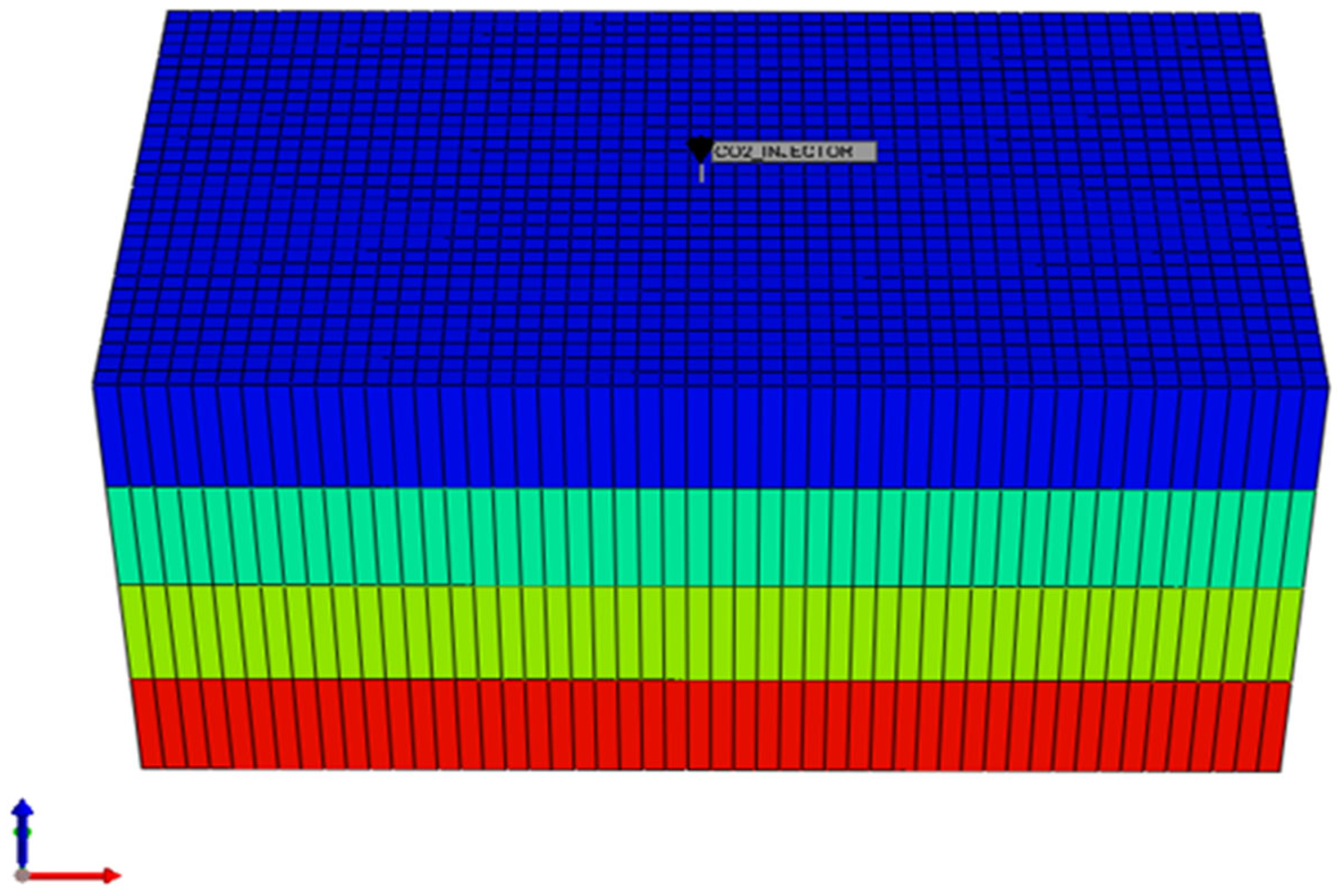
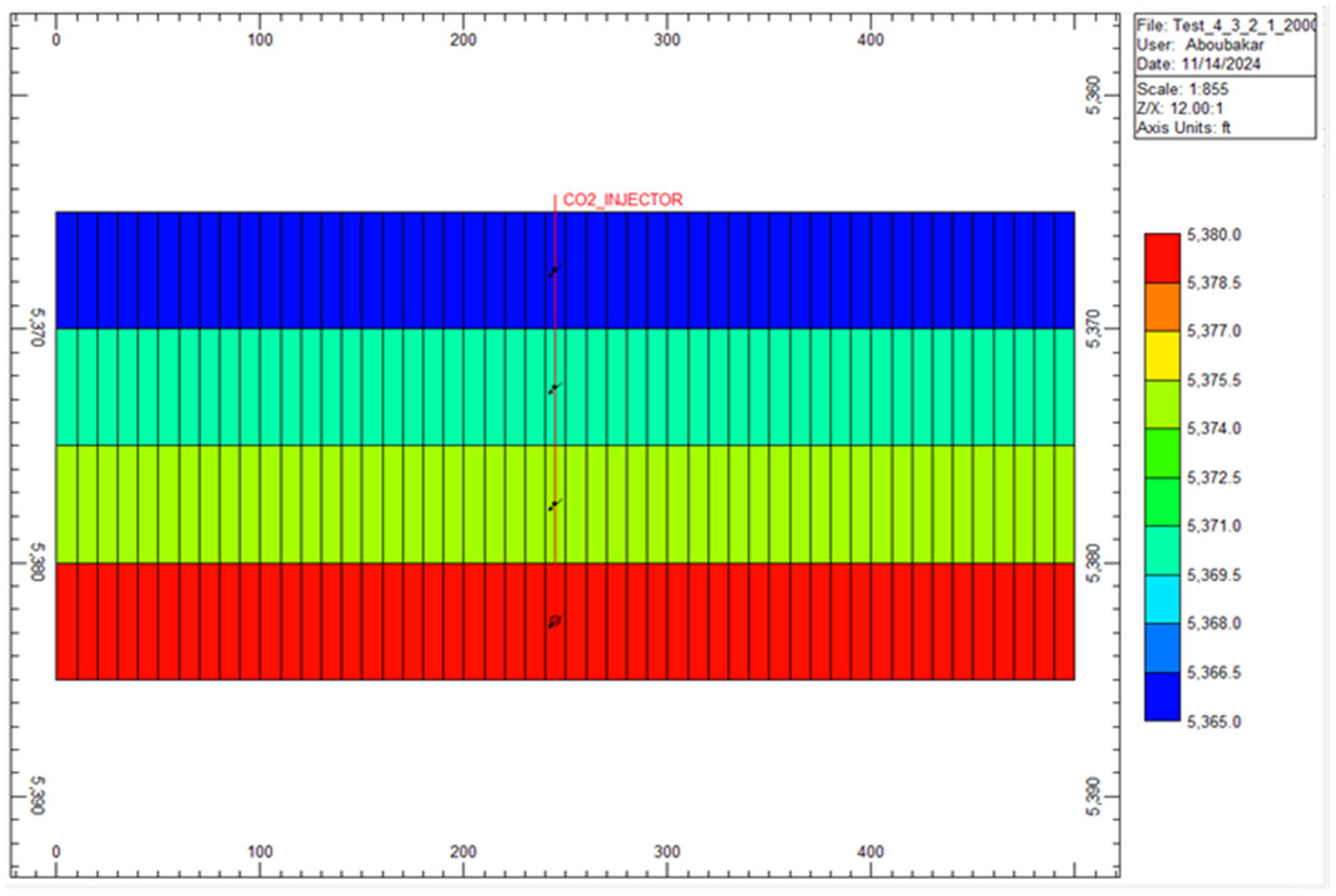
3.1. Model Setup and Grid Configuration

The model consists of a 3D grid with dimensions of 50 × 30 × 4 along the X, Y, and Z directions, respectively, with a width of 10 ft in all directions built with CMG 2021.10 software (Figure 2). This grid size was chosen to provide a sufficiently large area for observing horizontal migration patterns while maintaining a manageable number of cells for computational efficiency. The grid depth to the top is set at a depth of 5365 ft to reflect the conditions typical of the Illinois Basin Decatur Project’s geological setting. The four vertical layers in the grid allow CO₂ injection at varying depths (5370 ft, 5375 ft, 5380 ft, and 5385 ft), enabling an assessment of how injection depth influences the horizontal spread and trapping of CO₂ within the aquifer.

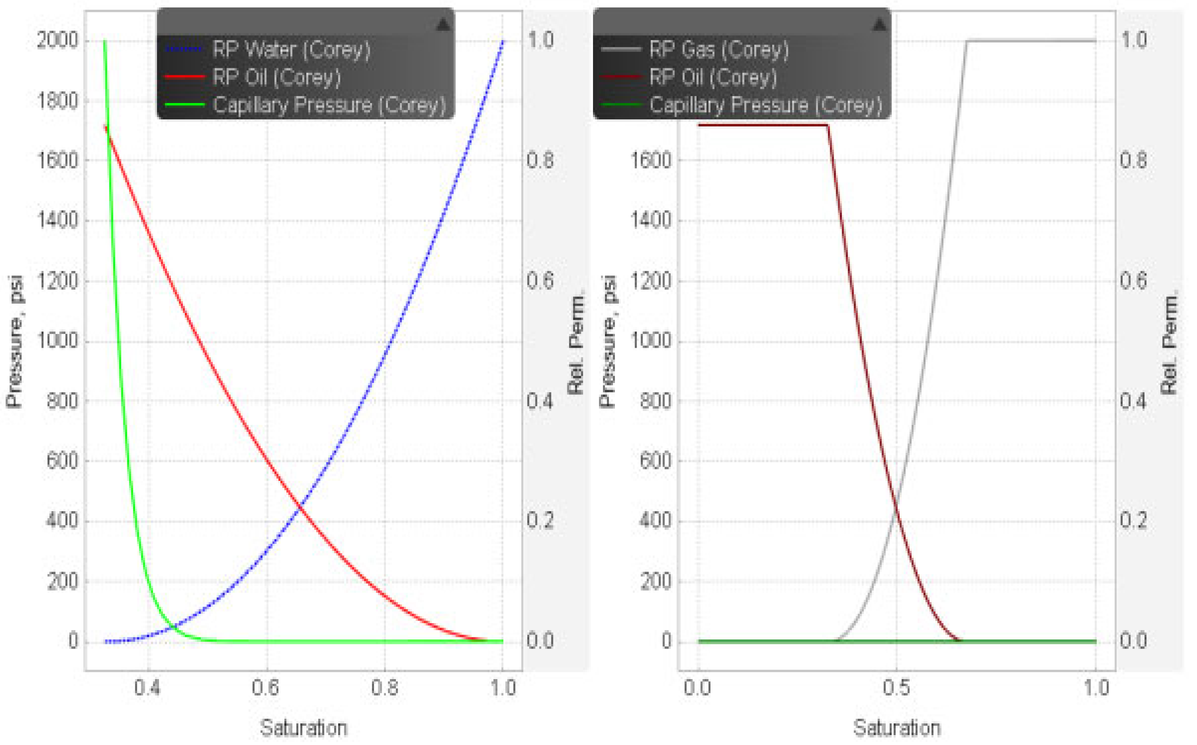
3.2. Reservoir Properties

Reservoir PVT, rock, and rock/fluid property (Figure 3) data are based on the Illinois Basin Decatur Project’s parameters, ensuring that the model closely resembles real-world CO₂ storage conditions. The horizontal permeability (k_x and k_y) is set to 200 millidarcies (mD) to permit significant horizontal CO₂ migration, while vertical permeability (k_z) is set to 20 mD, which restricts vertical movement and promotes horizontal dispersion of the plume. The uniform porosity of 30% across the grid cells reflects the average porosity observed in the Illinois Basin, contributing to consistent storage ability within the bearing saline formation. Additionally, the reservoir temperature is set at 112 °F, the reference pressure is 3205 psi, and the rock compressibility is 3.2 × 10⁻⁶ 1/psi.

3.3. Aquifer Salinity Level and Aqueous Phase Components

These salinity levels correspond to the concentration of dissolved salts, primarily in the form of ions such as Na⁺ (sodium) and Cl⁻ (chloride). The simulator allows the following components to participate in the aqueous reactions:

H₂O ⟷ H⁺ + OH⁻

CO₂ + H₂O ⟷ H⁺ + HCO⁻³

NaHCO₃ ⟷ HCO⁻³ + Na⁺

NaCl(s) ⟷ Na⁺ + Cl⁻

CaCO₃(s) + H⁺ ⟷ Ca²⁺ + HCO⁻³

3.4. CO₂ Injection Parameters

Supercritical CO₂ was injected at a constant rate of 35,000 scf/day for three years to ensure a controlled comparison of injection performance at varying depths. Injection occurred at four discrete depths, 5370 ft, 5375 ft, 5380 ft, and 5385 ft, corresponding to the center of each of four distinct grid layers (Figure 4). This relatively small depth variation was selected to evaluate the influence of initial pressure and temperature conditions on CO₂ migration while maintaining the CO₂ in a dense, supercritical state to minimize buoyancy effects. Following the injection period, each simulation included a post-injection monitoring phase to track residual CO₂ migration and assess long-term containment dynamics as the plume stabilized and interacted with the brine.

Table 1. Model parameter summary.

Parameters	Values	Units
Grid Size	50 × 30 × 4	block
Block Size	10	ft
Total Blocks	6000
Total Volume	6 × 106	ft3
Porosity	30	%
Pore Volume	9 × 105	ft3
Permeability X/Y/Z	200/200/20	mD
Rock Compressibility	3.2 × 10−6	psi−1
Initial Temperature	112	°F
Initial Pressure	3205	psi
Grid Top Depth	5365	ft
Brine Salinity	10 k/20 k	ppm
Injection Rate	350,000	scf
Injector Well Diameter	0.625	ft
Top Perforation	5370	ft
Injector Address	25 15 4/3/2/1	block
Maximum Injection Pressure	4000	psi
Max STG	350,000	ft3/day
Injection Period	3	years
Shut-in Period	197	years
Simulation Period	200	years
Reservoir Fluid	Brine
Injected Fluid	CO2	100%
Max Change Pressure	30,000	psi
Max Change Saturation	0.999
Max Change Global Composition	0.99

summarizes the model parameters.

3.5. Simulation Process and Data Collection

The simulation of CO₂ injection and migration in saline aquifers incorporates multiple equations; these equations collectively simulate how CO₂ interacts with brine, migrates within the aquifer, and undergoes various trapping mechanisms. The following are the key equations and processes used during simulation and data collection:

• Steady-state Aquifer:

This model assumes that the pressure at the external boundary of the aquifer does not change.

Then, the rate of water influx is

$$Q_{A }=C_A\left(p_A^{\left(i\right)}-\overline{p}\right)$$

where C_A = total compressibility of the aquifer, $p_A^{\left(i\right)}$ = pressure at the external boundary of the aquifer, and $\overline{p}$= average pressure at the aquifer–reservoir interface.

• Well Model:

The well model is an extension of the approach proposed by Peaceman [18,19] for both square and non-square gridblocks. The treatment of mobility adheres to the method suggested by Chappelear and Williamson [20]. Furthermore, the geometric factor enables the calculation of the equivalent radius based on the gridblock’s geometry and the well’s position within it. The injection well model establishes a relationship between the reservoir flow rate of phase $j$, the wellbore pressure $p_{bh}$, and the pressure at the grid point as follows:

$$Q_j={\sum }_{j}W{I}_j{\lambda }_{T,j}\left(p_{bh}-p_{o,i}\right) j=g,w$$

$$W{I}_j=2 \pi ff kh {\displaystyle \frac{wfrac}{\ln \left(\frac{r_e}{r_w}\right)+S}} j=g,w$$

where $Q_j$ = flow rate of phase j (j = g,w) at reservoir conditions (ft³/day), $W{I}_j$ = well injectivity index, ${\lambda }_{T,j}$ = total mobility of the fluid in the well block, $p_{bh}$ = bottomhole pressure (kPa | psia), $p_{o,i}$ = pressure of $i$th gridblock containing the well (kPa | psia), $ff$ = fraction of completion of the well in the gridblock, $k$ = effective permeability in the plane perpendicular to the well direction, $h$ = gridblock thickness in the well direction (m | ft), $wfrac$ = well fraction governed by areal geometry, $r_e$ = effective radius (m ft), $r_w$ = wellbore radius (ft), and S = skin factor.

• Pressure Loss Equation:

The wellbore model is an adaptation of the method by Aziz et al. [21], incorporating modifications that utilize an EOS to determine the phase behavior and fluid properties of the flowing fluid. The equation that describes the pressure variation $∆p$ along the flow direction in the wellbore model is

$$∆p={∆p}_H-∆p_{KE}-∆p_F$$

where $∆p_H=\rho g∆z$ is the hydrostatic pressure, $∆p_{KE}=-\rho v^2\ln \left({\displaystyle \frac{p_2}{p_1}}\right)$ is the kinetic energy gain, and $∆p_{F }={\displaystyle \frac{2 f^2{v}^2\rho }{D}}∆z$ is the friction gain. Here, ρ = density of the flowing “in situ” mixture, $g$ = acceleration due to gravity, f = fanning friction factor, $v$ = average velocity of the mixture, $D$ = inside pipe diameter, and $∆p$ = $p_2$ − $p_1$ = pressure drop over the length $∆z$.

• Partial Molar Volume Equation:

For CO₂, an internally developed correlation that aligns with the experimental data from Duan and Sun [22,23] is applied:

$${\overline{v}}_{\mathrm{C}\mathrm{O}2}\left({\mathrm{cm}}^3/\mathrm{mol}\right)=-47.75418+4.336154\times {10}^{-1}\times T-5.945771\times {10}^{-4}\times T^2$$

where T is the temperature in °C.

• Effect of Salinity:

The salting-out coefficient used is defined by the following relationship between Henry’s constant in pure water and in brine [24]:

$${\log }_{10}\left({\displaystyle \frac{H_{salt,i}}{H_i}}\right)=k_{salt,i} m_{salt}$$

where $H_{salt,i}$ = Henry’s constant of component $i$ in brine (salt solution), $H_i$ = Henry’s constant of component $i$ at zero salinity, $k_{salt.i}$ = salting-out coefficient for component $i$, and $m_{salt}$ = molality of the dissolved salt (mol/kg H₂O).

Bakker [25] provides the following correlations for the salting-out coefficients of CO₂ and CH₄, based on the data from Cramer [24]:

$$k_{salt,\mathrm{C}\mathrm{O}2}=0.11572-6.0293\times {10}^{-4} \widehat{T}+3.5817\times {10}^{-6}{\widehat{ T }}^2-3.7772\times {10}^{-9} {\widehat{T}}^3$$

where $\widehat{T }$ is the temperature in °K.

• Darcy’s Law for Multiphase Flow:

Darcy’s Law governs the flow velocities of each phase (CO₂ and brine) through the porous media of the saline aquifer, based on the formation’s permeability, viscosity, and pressure gradients:

$$V_{\alpha }=- {\displaystyle \frac{k{k}_{r\alpha }}{{\mu }_{\alpha }}}(\nabla P_{\alpha }-{\rho }_{\alpha }g\nabla z)$$

where $k$ = absolute permeability of the formation, $k_{r\alpha }$ = relative permeability of phase $\alpha$ (varies with saturation), ${\mu }_{\alpha }$ = viscosity of phase $\alpha$ (affected by salinity and temperature), ∇Pα = pressure gradient of phase $\alpha$, and ${\rho }_{\alpha }$ = density of phase $\alpha$.

• Peng–Robinson Equation of State (EOS) for Phase Behavior:

The Peng–Robinson EOS is used to model the phase behavior of CO₂ under high-pressure, high-temperature conditions, allowing the simulator to account for CO₂ properties in the supercritical and gaseous states:

$$P={\displaystyle \frac{RT}{V_m-b}}-{\displaystyle \frac{a\alpha }{\left(V_m^2+2b{V}_m-b^2\right)}}$$

where $R$ = 8.314 J/mol. K, $V_m$ = molar volume of CO₂ or brine phase, a = attraction parameter, and $b$ = repulsion parameter.

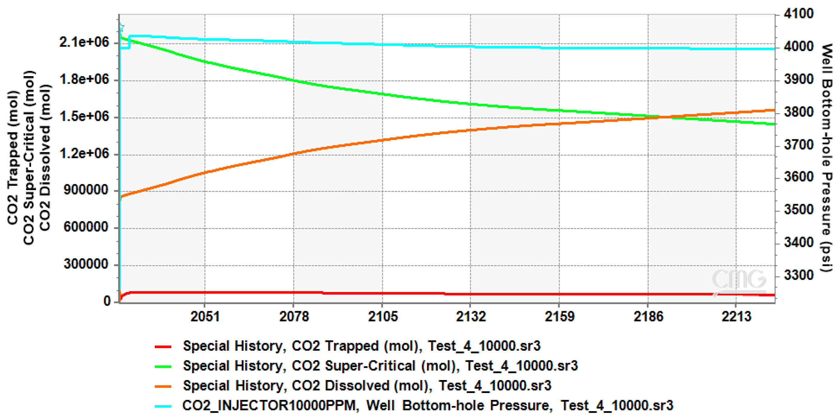
4. Results and Discussion

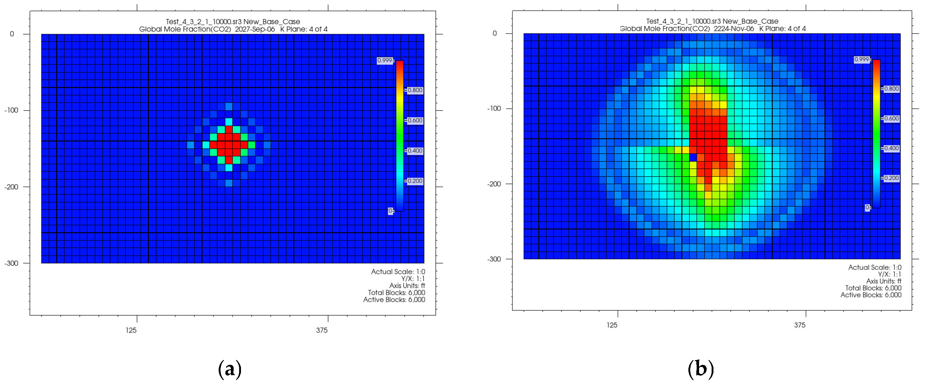
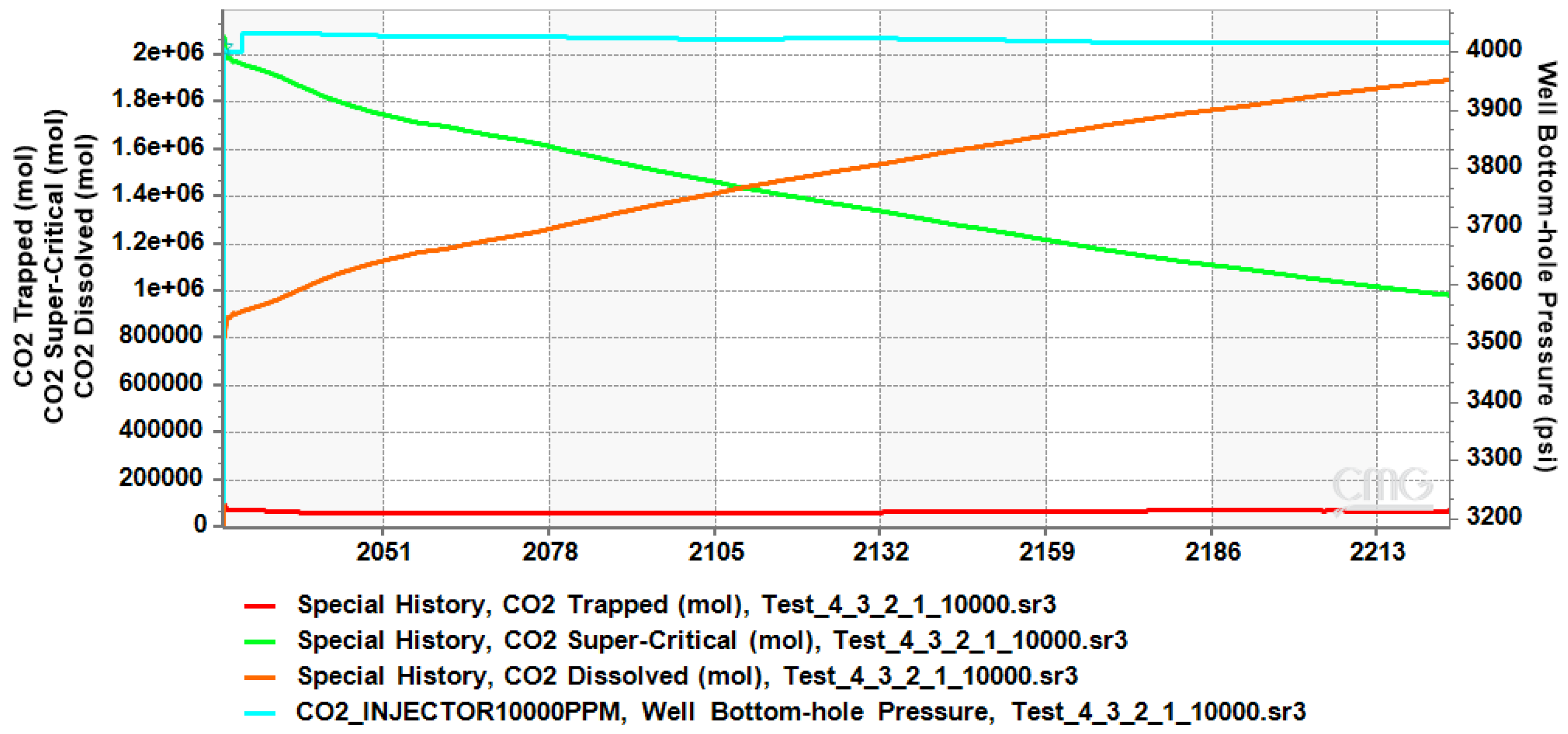
4.1. CO₂ Plume Migration in Layer 4 (Bottom Layer)

With the largest CO₂ mole fractions concentrated close to the wellbore (around 0.99), the plume in this instance exhibits a radial spread centered around the injection site, progressively declining outward (Figure 5). According to this gradient, dissolution trapping becomes increasingly important toward the edges of the plume, whilst CO₂ is mostly in a supercritical phase close to the injection site. The sustained saturation levels in the outer plume regions are a result of increased dissolution trapping caused by the reduced salinity, which also increases CO₂ solubility in brine. A significant amount of CO₂ has changed into a dissolved state, stabilizing the horizontal spread of the plume, as evidenced by the trapping mechanisms graph, which displays a consistent increase in dissolved CO₂ over time.

The residually trapped CO₂ continues to increase steadily after 2007 days, reaching a peak of 84,854 moles. This can be attributed to the dissipation of the pressure buildup created during the injection phase once injection ceases. As the pressure decreases, brine from surrounding areas flows back toward the injection site, and this backflow effectively traps the CO₂ in the pore throats of the reservoir. When mineral and dissolution trapping mechanisms take effect, residual trapping starts decreasing, reaching 66,080 moles at the end of the simulation period. The supercritical CO₂ fraction starts high at approximately 2.2 million moles but decreases gradually, reflecting a phase transition or dissolution into the aqueous phase, reaching about 1.4 million moles. Conversely, the CO₂ dissolved in the formation shows a significant increase, starting at zero and rising to over 1.56 million moles, highlighting the active role of solubility trapping in long-term storage. The decreasing slope of the dissolved CO₂ curve over time may result from the brine gradually reaching saturation with CO₂, which limits the rate of further dissolution. In addition, the salting-out effect may limit CO₂ solubility due to increased ionic strength in the brine.

The well bottomhole pressure (BHP) starts at 4037 psi and shows a slight but consistent decrease, reaching 3998 psi, suggesting effective pressure dissipation in the reservoir. The interplay between trapped, supercritical, and dissolved CO₂ emphasizes the reservoir’s capacity to transition between different trapping mechanisms, ensuring effective and secure CO₂ storage. These trends confirm the reservoir’s ability to immobilize CO₂ securely, with a balance between residual and solubility trapping (see Figure 6). The total trapped CO₂ in this case is 1.63 million moles.

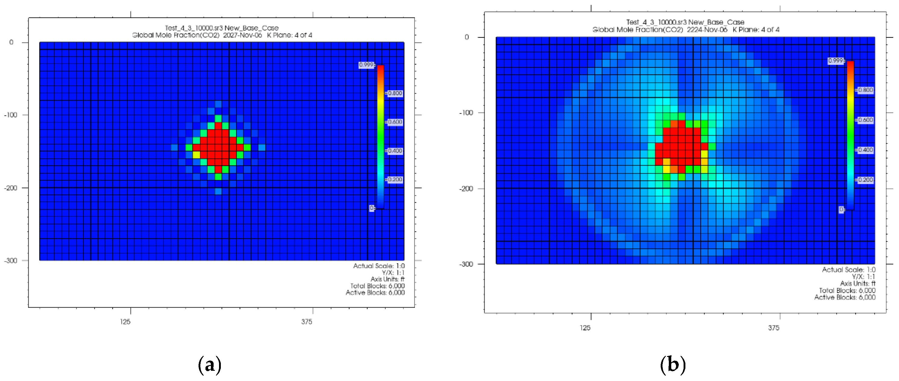
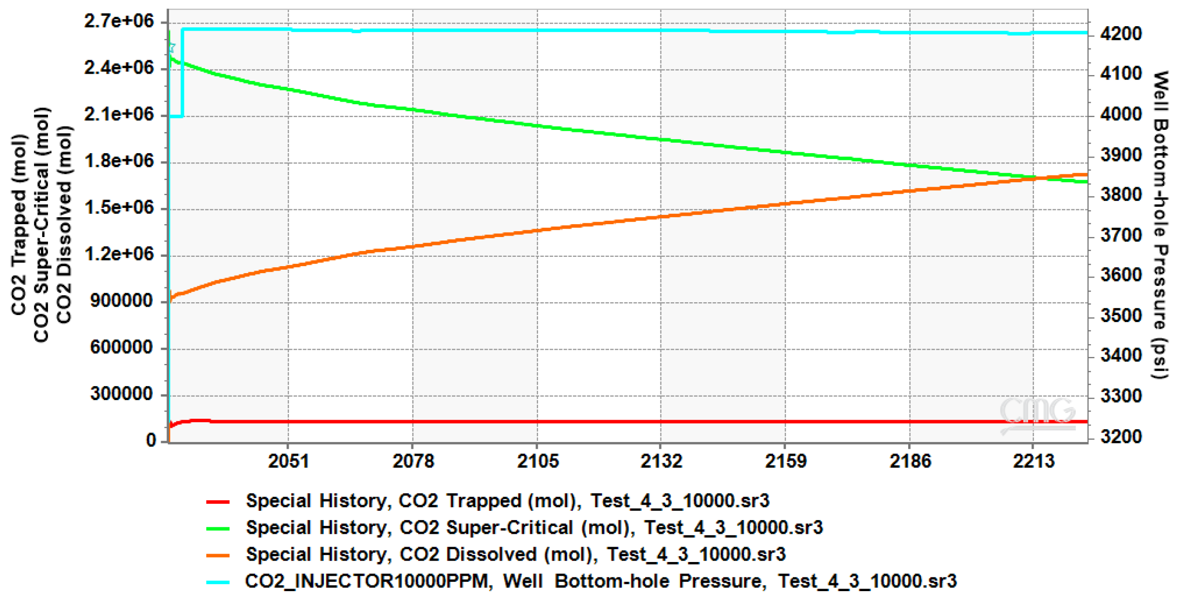
4.2. CO₂ Plume Migration in Layers 3 and 4

Because of the combined pressure fields from each injection point, the simulation results show a compact, merged plume structure with CO₂ injectors operating at injection depths of 5380 and 5385 feet (layer 3 and 4), see Figure 7. Effective confinement through dissolution trapping is suggested by the plume image’s high CO₂ mole fraction concentrated close to the injection zone, approaching 0.99, which progressively drops outward. The comparative salinity of 10,000 ppm improves this trapping by making CO₂ more soluble, which permits more CO₂ to dissolve into the brine as it spreads out from the injection point. A consistent CO₂ distribution is produced at 5380 and 5385 feet. This is characterized by the overlapping pressure fields at both depths, stabilizing the plume boundary and reducing both vertical and horizontal migration. The graph of the trapping mechanisms supports this containment: the dissolved CO₂ steadily rises and plateaus, indicating near-saturation in the brine, while supercritical CO₂ declines as it transitions into more stable dissolved and trapped states. Residual trapping, shown in the graph, is low but stable, adding to long-term containment by immobilizing CO₂ in pore spaces.

The efficiency of residual trapping mechanisms is demonstrated by the amount of CO₂ trapped, which starts at 0 mol and climbs gradually during the simulation before stabilizing at about 134,000 moles. After beginning at a high value of more than 2.4 million moles, the supercritical CO₂ progressively drops to about 1.68 million moles, signaling a switch to different trapping methods such as solubility trapping. The predominant long-term storage mechanism, solubility trapping, is highlighted by the fact that dissolved CO₂ rises quickly, eventually surpassing supercritical CO₂ and reaching 1.7 million moles. This is 200,000 more moles of dissolved CO₂ than in the previous case. The BHP decreases from about 4216 psi to 4208 psi, suggesting slow pressure dissipation in the reservoir. This modest reduction is possibly due to CO₂ migration and trapping mechanisms balancing the injection rates (see Figure 8). In this case, the total trapping mechanisms trapped 1.83 million moles of CO₂.

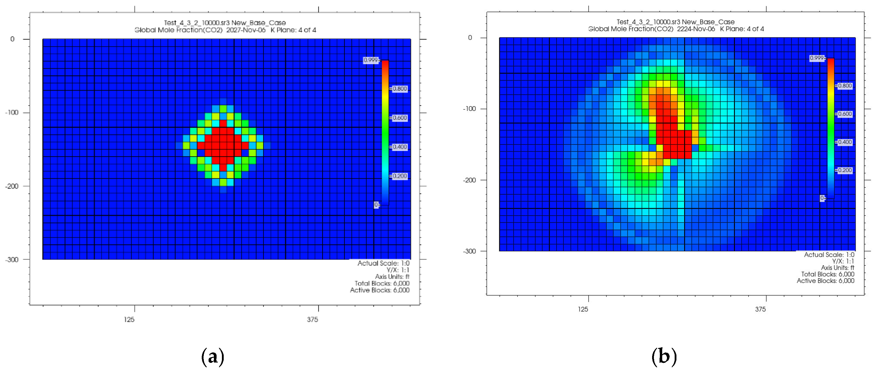
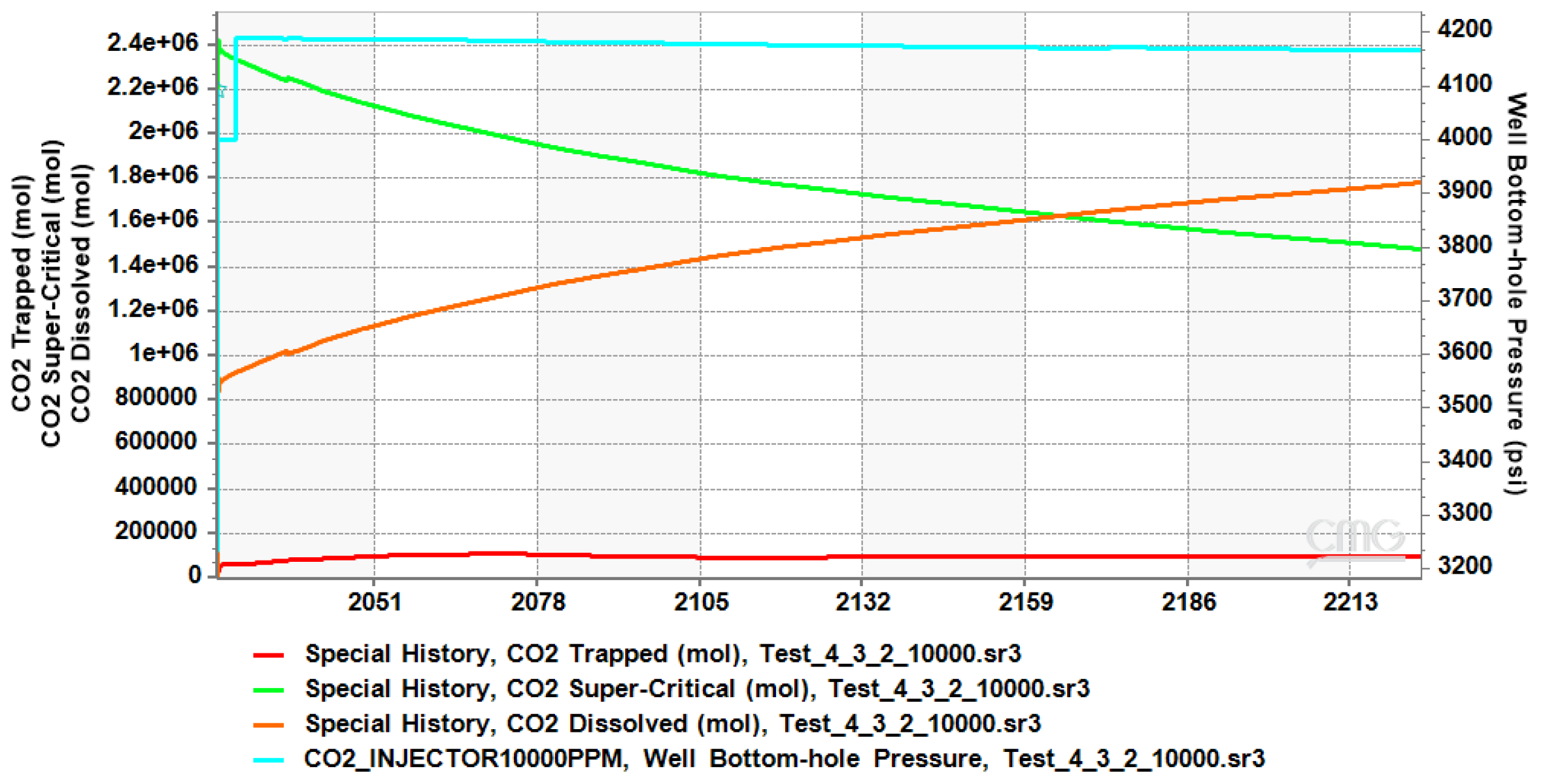
4.3. CO₂ Plume Migration in Layers 2, 3, and 4

Compared to the prior completion options, the plume shows larger horizontal migration (Figure 9), where CO₂ is injected in layers 2 to 4, at depths of 5385, 5380, and 5375 feet. This is because the combined pressure from several depths causes the plume to extend horizontally. A more uniform horizontal distribution generated by cumulative pressure across the three injection spots is indicated by the plume image’s high CO₂ mole fraction of 0.99 near the injection area, which tapers to about 0.2–0.4 at the edges. As the CO₂ plume encounters a larger volume of brine, the graph shows that the dissolved CO₂ rises to about 1.8 million moles, a steeper rise than in the case of injecting in only layers 3 and 4. These results highlight improved dissolution trapping. Supercritical CO₂, tracked by the green line, decreases from about 2.3 million moles initially to around 1.4 million moles, suggesting that the broader horizontal spread facilitates the transition of CO₂ into dissolved and residually trapped states.

The sensitivity analysis of CO₂ trapped and bottomhole pressure (BHP) over the simulation period reveals key insights into reservoir behavior. The CO₂ residual trapped starts at 60,731 moles and steadily increases throughout the simulation, reaching a maximum of 107,112 moles in 2027. It then decreases, reaching a minimum of 98,700 moles in 2224, demonstrating effective residual and mineral trapping mechanisms. Meanwhile, the BHP begins at 4184 psi; toward the end of the simulation, the BHP decreases slightly, stabilizing at 4166 psi, indicating slight pressure dissipation within the reservoir. We noticed a total of 1.78 million moles of CO₂ dissolved, 80,000 more moles than in the previous case. The supercritical CO₂ dropped to reach 1.46 million moles, a decrease of 220,000 moles compared to the previous case (see Figure 10), leading to a total sequestration of 1.88 million moles of CO₂.

4.4. CO₂ Plume Migration in Layers 1 Through 4

The horizontal movement of the plume is more noticeable with CO₂ injected in layers 1 through 4 (Figure 11). The pressure field is expanded both horizontally and vertically by the additional injection point at 5370 feet, which promotes the spread of CO₂. With CO₂ mole fractions progressively dropping from a peak of 0.99 close to the injection locations to roughly 0.04 at the outside borders, the plume propagation figure displays a wider horizontal spread. A larger, more cohesive pressure field produced by the additional injectors pushes CO₂ farther outward, lowering the concentration gradient and enabling more extensive interaction between the CO₂ and the surrounding brine. This is demonstrated by the enlarged horizontal migration. The greater brine contact area and higher dissolution trapping effectiveness over the larger containment zone are reflected in the graph, which supports this improved horizontal spread as the amount of dissolved CO₂ reaches 1.9 million moles. The total residually trapped CO₂ is 69,080 moles. This horizontal movement causes additional CO₂ to go into dissolved phases, as evidenced by the amount of supercritical CO₂ dropping from 2.4 million moles to 1 million moles.

The well bottomhole pressure stabilizes at around 4000 from 4031 psi, maintaining a stable containment field across the larger horizontal area but allowing for greater horizontal distribution than in the three-injector case, where the plume was more compact. Completing layers 1 through 4 maximizes horizontal migration, enhancing CO₂ trapping across a broader area while achieving a stable containment field with a reduced likelihood of vertical migration (see Figure 12). In our last case, we had a total of 1,969,080 moles of trapped CO₂.

Multi-layer completion significantly enhances CO₂ sequestration compared to single-layer injection. Simultaneous injection at four depths (5370 ft, 5375 ft, 5380 ft, and 5385 ft) maximized CO₂ storage, achieving approximately 2 million moles, with dissolution trapping accounting for 96% of the total during the simulation period. This multi-layer approach resulted in a 1.2-fold increase in sequestration capacity relative to single-depth injection. The improvement is attributed to the increased interfacial contact area between CO₂ and brine, which promotes dissolution and reduces the volume of buoyant supercritical CO₂. The relatively high CO₂ solubility in the 10,000 ppm brine further facilitates dissolution and minimizes the potential for lateral or upward plume migration. The observed deviation from a perfectly circular plume is attributed to vertical migration, likely influenced by the relatively low vertical permeability (20 mD). This result is consistent with previous research by Hassan et al. [26], which demonstrated that multi-layer injection in idealized aquifer systems enhances CO₂ storage capacity by distributing the injected fluid across multiple zones, increasing the CO₂–brine contact area and promoting dissolution trapping.

Despite these promising results, several potential limitations and uncertainties in the study warrant consideration. First, the results rely on specific assumptions about reservoir properties, such as permeability, porosity, and brine salinity. Variations in these parameters could significantly impact CO₂ storage efficiency, plume behavior, and dissolution rates. Conducting sensitivity analyses in future studies would help quantify the effect of these parameter variations on the outcomes. Then, this study assumes homogeneous aquifer properties, such as uniform permeability (along the X and Y directions) and salinity. In reality, aquifers are often highly heterogeneous, which can lead to more complex CO₂ plume behavior and storage dynamics. Incorporating reservoir heterogeneity into the simulation framework could provide more accurate and realistic predictions. Finally, the boundary conditions used in the model might not perfectly represent the extent of the reservoir or its interaction with neighboring formations. Simplifying the reservoir boundaries could lead to deviations between simulated results and actual field performance. Considering more complex boundary conditions and scaling effects would enhance the model’s applicability to real-world scenarios.

5. Conclusions

This study investigated multi-layer CO₂ injection for enhanced sequestration in a 10,000 ppm salinity saline aquifer. The results demonstrate that simultaneous injection at four depths (5370–5385 ft) maximized CO₂ storage, achieving approximately 2 million moles, with dissolution trapping accounting for 96% of the total during the simulation. This multi-layer approach yielded a 1.2-fold increase in sequestration capacity compared to single-depth injection, attributed to increased CO₂–brine contact, and promoted dissolution, consistent with the findings of Hassan et al. [26]. However, the study relies on simplifying assumptions regarding reservoir properties (e.g., homogeneity, constant permeability, and salinity) and boundary conditions, which could impact the accuracy of predictions. Future work should prioritize sensitivity analyses, incorporate reservoir heterogeneity, and consider more complex boundary conditions to enhance the model’s applicability to real-world scenarios.

References

1. Zhang, Y.; Jackson, C.; Krevor, S. The feasibility of reaching gigatonne scale CO2 storage by mid-century. Nat. Commun. 2024, 15, 6913. [Google Scholar] [CrossRef] [PubMed]
2. Zhou, Q.; Birkholzer, J.T.; Tsang, C.F.; Rutqvist, J. A method for quick assessment of CO2 storage capacity in closed and semi-closed saline formations. Int. J. Greenh. Gas Control 2008, 2, 626–639. [Google Scholar] [CrossRef]
3. Fominykh, S.; Stankovski, S.; Markovic, V. Analysis of CO2 migration in horizontal saline aquifers during carbon capture and storage process. Sustainability 2023, 15, 8912. [Google Scholar] [CrossRef]
4. Li, Q.; Han, Y.; Liu, X.; Ansari, U.; Cheng, Y.; Yan, C. Hydrate as a by-product in CO2 leakage during the long-term sub-seabed sequestration and its role in preventing further leakage. Environ. Sci. Pollut. Res. 2022, 29, 77737–77754. [Google Scholar] [CrossRef]
5. Jing, J.; Yang, Y.; Cheng, J.; Ding, Z. Exploring the influences of salinity on CO2 plume migration and storage capacity in sloping formations: A numerical investigation. Energy 2024, 309, 133160. [Google Scholar] [CrossRef]
6. Sun, X.; Cao, Y.; Liu, K. Effects of fluvial sedimentary heterogeneity on CO2 geological storage: Integrating storage capacity, injectivity, distribution, and CO2 phases. J. Hydrol. 2023, 617, 128936. [Google Scholar] [CrossRef]
7. Al-Khdheeawi, E.; Vialle, S.; Barifcani, A.; Sarmadivaleh, M.; Zhang, Y.; Iglauer, S. Impact of salinity on CO2 containment security in highly heterogeneous reservoirs. Greenh. Gases Sci. Technol. 2017, 8, 1723. [Google Scholar]
8. Al-Khdheeawi, E.; Vialle, S.; Barifcani, A.; Sarmadivaleh, M.; Zhang, Y.; Iglauer, S. Influence of injection well configuration and rock wettability on CO2 plume behaviour and CO2 trapping capacity in heterogeneous reservoirs. J. Nat. Gas Sci. Eng. 2017, 3, 16. [Google Scholar]
9. Kumar, S.; Foroozesh, J.; Edlmann, K.; Rezk, M.; Lim, C. A Comprehensive Review of Value-Added CO2 Sequestration in Subsurface Saline Aquifers. J. Nat. Gas Sci. Eng. 2020, 81, 103437. [Google Scholar] [CrossRef]
10. Okwen, R.T.; Stewart, M.T.; Cunningham, J.A. Analytical solution for estimating storage efficiency of dissolved and residual CO2 in saline aquifers. Int. J. Greenh. Gas Control 2010, 4, 102–107. [Google Scholar] [CrossRef]
11. Liu, E.; Lu, X.; Wang, D.A. Systematic Review of Carbon Capture, Utilization and Storage: Status, Progress and Challenges. Energies 2023, 16, 2865. [Google Scholar] [CrossRef]
12. Xu, T.; Apps, J.A.; Pruess, K.; Yamamoto, H. Numerical modeling of injection and mineral trapping of CO2 with H2S and SO2 in a sandstone formation. Chem. Geol. 2007, 242, 319–346. [Google Scholar] [CrossRef]
13. Osborn, N.I.; Smith, S.J.; Seger, C.H. Hydrogeology, Distribution, and Volume of Saline Groundwater in the Southern Midcontinent and Adjacent Areas of the United States. US Geol. Surv. 2013, 15, 16–17. [Google Scholar]
14. Yang, D.; Liu, N.; Gu, Y. Enhanced mass transfer for CO2 sequestration in saline aquifers. Ind. Eng. Chem. Res. 2005, 44, 2164–2174. [Google Scholar]
15. Yang, Y.; Xu, T.; Wang, F.; Zhao, N. Impact of inner reservoir faults on migration and storage of injected CO2. Int. J. Greenh. Gas Control 2021, 72, 14–25. [Google Scholar] [CrossRef]
16. Hovorka, S.D.; Meckel, T.A.; Treviño, R.H. Monitoring a large-volume injection at Cranfield, Mississippi Project design and recommendations. Int. J. Greenh. Gas Control 2013, 18, 345–360. [Google Scholar] [CrossRef]
17. Rathnaweera, T.D.; Ranjith, P.G. Effect of salinity on effective CO2 permeability in reservoir rock determined by pressure transient methods. Rock Mech. Rock Eng. 2023, 48, 2093–2110. [Google Scholar] [CrossRef]
18. Peaceman, D. Interpretation of well-block pressures in numerical reservoir simulation. In Proceedings of the 52nd Annual Fall Technical Conference and Exhibition, Denver, CO, USA, 9–12 October 1977. [Google Scholar]
19. Peaceman, D. Interpretation of well-block pressures in numerical reservoir simulation with non-square grid blocks and anisotropic permeability. Soc. Pet. Eng. J. 1983, 23, 531–543. [Google Scholar] [CrossRef]
20. Chappelear, J.; Williamson, A.E. Representing Wells in Numerical Reservoir Simulation: Part I—Theory Part II—Implementation. Soc. Pet. Eng. J. 1981, 21, 323–344. [Google Scholar] [CrossRef]
21. Aziz, K.; Govier, G.W.; Schowalter, W.R. The Flow of Complex Mixtures in Pipes. ASME J. Appl. Mech. 1973, 2, 404. [Google Scholar]
22. Duan, Z.; Sun, R.; Zhu, C.; Chou, I.M. An improved model for the calculation of CO2 solubility in aqueous solutions containing Na+, K+, Ca2+, Mg2+, Cl, and SO₄². Mar. Chem. 2006, 98, 131–139. [Google Scholar] [CrossRef]
23. Duan, Z.; Sun, R. An improved model calculating CO2 solubility in pure water and aqueous NaCl solutions from 273 to 533 K and from 0 to 2000 bar. Chem. Geol. 2003, 193, 257–271. [Google Scholar] [CrossRef]
24. Cramer, S. The Solubility of Methane, Carbon Dioxide, and Oxygen in Brines from 0 to 300 C; US Department of the Interior, Bureau of Mines: Washington, DC, USA, 1982. [Google Scholar]
25. Bakker, R. Computer programs for analysis of fluid inclusion data and for modelling bulk fluid properties. Chem. Geol. Chem. Geol. 2003, 194, 3–23. [Google Scholar] [CrossRef]
26. Hassan, W.; Jiang, X. Numerical Investigation of Multi-layer CO2 Injection in Deep Saline Aquifers with Improperly Abandoned Wells. Energy Procedia 2014, 61, 160–163. [Google Scholar] [CrossRef]
Figure 1. Dissolved solid concentrations and thickness in the Gulf Coast Regional Aquifer System [13].
Processes 13 00734 g001
Figure 2. Grid model.
Processes 13 00734 g002
Figure 3. Relative permeability curve from the IBDP (EDX 2021).
Processes 13 00734 g003
Figure 4. Vertical profile and injection depths.
Processes 13 00734 g004
Figure 5. Plume migration in layer 4 from shut-in (a) to the end of the simulation (b).
Processes 13 00734 g005
Figure 6. Trapped, supercritical, dissolved, and BHP profile of CO2 in layer 4.
Processes 13 00734 g006
Figure 7. Plume migration in layer 3 and 4 from shut-in (a) to the end of the simulation (b).
Processes 13 00734 g007
Figure 8. Trapped, supercritical, dissolved, and BHP profile of CO2 in layers 3 and 4.
Processes 13 00734 g008
Figure 9. Plume migration in layers 2, 3, and 4 from shut-in (a) to the end of the simulation (b).
Processes 13 00734 g009
Figure 10. Trapped, supercritical, dissolved, and BHP profile of CO2 in layers 2, 3, 4.
Processes 13 00734 g010
Figure 11. Plume migration in layer 1 through 4 from shut-in (a) to the end of the simulation (b).
Processes 13 00734 g011
Figure 12. Trapped, supercritical, dissolved, and BHP profile of CO2 in layer 1 through 4.
Processes 13 00734 g012